Abstract

In the dynamical gauge-Higgs unification of electroweak interactions in the Randall-Sundrum warped spacetime the Higgs boson mass is predicted in the range 120 GeV – 290 GeV, provided that the spacetime structure is determined at the Planck scale. Couplings of quarks and leptons to gauge bosons and their Kaluza-Klein (KK) excited states are determined by the masses of quarks and leptons. All quarks and leptons other than top quarks have very small couplings to the KK excited states of gauge bosons. The universality of weak interactions is slightly broken by magnitudes of $10^{-8}$, $10^{-6}$ and $10^{-2}$ for $\mu$-$e$, $\tau$-$e$ and $t$-$e$, respectively. Yukawa couplings become substantially smaller than those in the standard model, by a factor $|\cos\hbox{${1\over 2}$}\theta_{W}|$ where $\theta_{W}$ is the non-Abelian Aharonov-Bohm phase (the Wilson line phase) associated with dynamical electroweak symmetry breaking.

May 9, 2006 OU-HET 552/2006

1 Introduction

In the extra-dimensional gauge-Higgs unification the Higgs field is unified with the gauge fields so that the mass of the Higgs particle and its self-couplings and couplings to quarks and leptons are all determined by the underlying gauge principle and the structure of spacetime. As a bonus it serves as an alternative to minimal supersymmetric standard model to stabilize the Higgs field in the electroweak interactions. The gauge-Higgs unification in the Randall-Sundrum (RS) warped spacetime has attracted much attention for its phenomenological consequences.[2, 3] In particular the Higgs mass in the dynamical gauge-Higgs unification in the RS warped spacetime is predicted in the energy range 120 GeV - 290 GeV exactly where experiments at LHC can explore.[4] Predictions from the gauge-Higgs unification are not limited to the Higgs sector. The main purpose of the present paper is to show that there appears non-universality in the weak gauge coupling of quarks and leptons and the Yukawa couplings of quarks and leptons are substantially reduced in the extra-dimensional gauge-Higgs unification scheme. The deviation from the universality turns out to be small and is within the current experimental limit. It becomes larger for heavier leptons and quarks, and can be tested in future experiments. The reduction of the Yukawa couplings can be tested in experiments at LHC.

There are several key ingredients in the extra-dimensional gauge-Higgs unification. First, in the electroweak interactions the $SU(2)_{L}\times U(1)_{Y}$ symmetry breaks down to $U(1)_{EM}$ by nonvanishing vacuum expectation value of the doublet Higgs field. In the gauge-Higgs unification the 4D Higgs field is identified with the extra-dimensional component of the gauge potentials which is necessarily in the adjoint representation of the gauge group. It implies that one has to start with a larger gauge group such as $SU(3)$, $SO(5)$, and $G_{2}$ to accommodate the 4D Higgs field. This observation was made by Fairlie and by Forgacs and Manton.[5, 6] Secondly, dynamical mechanism for electroweak symmetry breaking in the gauge-Higgs unification is provided by quantum dynamics of non-Abelian Aharonov-Bohm phases (Wilson line phases), once the extra-dimensional space is non-simply connected.[7, 8] Classical vacua are degenerate along the direction of Wilson line phases. The degeneracy is lifted by quantum effects, thereby the gauge symmetry being spontaneously broken. This Hosotani mechanism also gives the 4D Higgs field a finite mass by radiative corrections[9].

The early attempt of dynamical gauge-Higgs unification, however, encountered severe difficulty in incorporating chiral fermions. A major breakthrough came in the last decade by considering an orbifold as extra-dimensional space.[10] The left-right asymmetry is naturally implemented in orbifold boundary conditions so that the matter content of the standard model appears in the effective theory at low energies.[11]-[18] The idea has been applied to grand unified theory as well.[19]-[22]

One of the necessary consequences of gauge-Higgs unification is that the property of the Higgs particle is mostly fixed by the gauge principle and the structure of the extra dimension. In particular, the $W$ boson mass ($m_{W}$), the Higgs boson mass ($m_{H}$), and the Kaluza-Klein mass scale ($m_{\rm KK}$) are related to each other. In the dynamical gauge-Higgs unification in flat space one finds that $m_{H}\sim\sqrt{\alpha_{W}}\,m_{W}/\theta_{W}$ where $\alpha_{W}=g_{SU(2)}^{2}/4\pi$ and $\theta_{W}$ is the Wilson line phase (the non-Abelian Aharonov-Bohm phase) associated with the VEV of the extra-dimensional component of gauge potentials. Natural matter content yields $\theta_{W}$ in the range $0.2\pi$ - $0.5\pi$ so that $m_{H}$ is found to be too small ($\sim 10$ GeV). Further $m_{\rm KK}$ turns to be $\sim(2\pi/\theta_{W})m_{W}$, which also contradicts with experimental limits. It is not impossible to engineer a model such that the resultant $\theta_{W}$ becomes small enough to make the Higgs particle sufficiently heavy, but it requires artificial tuning of matter content.[14, 15, 17, 18]

It has been recognized that a much better and natural way of having more realistic phenomenology in gauge-Higgs unification is to consider gauge theory in curved spacetime. In particular, in the Randall-Sundrum (RS) warped spacetime[23] an enhancement factor resulting from the spacetime curvature leads to $m_{H}=(120\sim 290)$ GeV, just the mass value to be tested at LHC. The Kaluza-Klein mass scale turns to be 1.5 TeV to 3.5 TeV as well.

The consequences of gravitational effects in the gauge-Higgs unification are far-reaching. On an orbifold with topology $S^{1}/Z_{2}$ each fermion multiplet can have its own bulk kink mass $M$. In the RS spacetime, in particular, there results a natural dimensionless parameter $M/k$ where $k$ is related to the cosmological constant $\Lambda=-k^{2}$ in the bulk. These parameters are fixed by $m_{W}$ and quark/lepton masses, which in turn determine wave functions of quarks and leptons in the fifth dimension. Couplings of quarks and leptons to gauge bosons, the Higgs boson, and their Kaluza-Klein towers are unambiguiously determined. This procedure of calculating various couplings is previously performed in Ref.[24] although their context is not exactly the gauge-Higgs unification. Most of our results qualitatively reproduce their results as expected. However there are some consequences inherent in the gauge-Higgs unification in the RS spacetime. We will find that the universality of the weak interactions is slightly broken, which can be tested by future experiments. Further the 4D Yukawa couplings of quarks and leptons are substantially reduced.

Gauge theory in the RS spacetime has been under intensive investigation.[25]-[28] The RS geometry gives a natural bridge between the Planck scale (gravitational scale) and the weak scale by a warp factor. The geometry in the fifth dimension is anti-de Sitter, which enables the gauge-Higgs unification in the RS spacetime to have intriguing interpretation in the AdS/CFT correspondence.[2, 3] We will see that dynamical gauge symmetry breaking in the RS spacetime by the Hosotani mechanism leads to intricate structure in the electroweak interactions in the quark-lepton sector. The key is the observed quark-lepton mass spectrum, from which the fine structure in the gauge couplings and the Higgs couplings is unambiguiously determined for experimental verification.

In this paper we consider an $SU(3)$ gauge theory as an example. This model has been extensively studied in flat space for simplicity. It is well known, however, that the $SU(3)$ model does not give realistic structure in the neutral current sector. In particular, the Weinberg angle in the model turns out too big. With this limitation in mind, we do not address the issue of non-universality in neutral current interactions. To have realistic structure in neutral current, extension of gauge group to, say, $SO(5)\times U(1)_{B-L}$ is necessary as discussed in Ref.[3]. It is anticipated that most of the qualitative features obtained in the present paper remain valid in such modified models as well.

In section 2 gauge theory in the RS spacetime is specified with boundary conditions. In sections 3 and 4 all fields are expanded around a nontrivial background of the Wilson line phase, and spectra and mode functions in the fifth dimension are obtained. General features of the mass spectra are clarified in section 5. The bulk mass parameters of quarks and leptons are related to their observed masses. The mass and self-couplings of the Higgs field are also determined there. Nontrivial behavior of gauge couplings of quarks and leptons is investigated in section 6, and the non-universality of weak interactions is established. Reduction of Yukawa couplings of quarks and leptons is shown in section 7. Section 8 is devoted to conclusion and discussions. Useful formulae are summarized in appendices.

2 Gauge theory in the RS spacetime

We consider an $SU(3)$ gauge theory on the Randall-Sundrum geometry [23]. The fifth dimension is compactified on an orbifold $S^{1}/Z_{2}$ with a radius $R$. The bulk five-dimensional spacetime has a negative cosmological constant $-k^{2}$. We use, throughout the paper, $M,N,\cdots=0,1,2,3,4$ for the 5D curved indices, $A,B,\cdots=0,1,2,3,4$ for the 5D flat indices in tetrads, and $\mu,\nu,\cdots=0,1,2,3$ for 4D indices. The background metric is given by

$$ds^{2}=G_{MN}dx^{M}dx^{N}=e^{-2\sigma(y)}\eta_{\mu\nu}dx^{\mu}dx^{\nu}+dy^{2},$$ (2.1)

where $\eta_{\mu\nu}={\rm diag~{}}(-1,1,1,1)$, $\sigma(y)=\sigma(y+2\pi R)$, and $\sigma(y)\equiv k\left|y\right|$ for $|y|\leq\pi R$ with $k$ being the inverse AdS curvature radius.

The field content consists of $SU(3)$ gauge boson

$$A_{M}=\sum_{a=1}^{8}A_{M}^{a}\frac{\lambda^{a}}{2}=\frac{1}{2}\left(\begin{array}[]{ccc}A^{3}_{M}+\frac{1}{\sqrt{3}}A^{8}_{M}&A^{1}_{M}-iA^{2}_{M}&A^{4}_{M}-iA^{5}_{M}\\ A^{1}_{M}+iA^{2}_{M}&-A^{3}_{M}+\frac{1}{\sqrt{3}}A^{8}_{M}&A^{6}_{M}-iA^{7}_{M}\\ A^{4}_{M}+iA^{5}_{M}&A^{6}_{M}+iA^{7}_{M}&-\frac{2}{\sqrt{3}}A^{8}_{M}\end{array}\right),$$ (2.2)

the corresponding ghost fields $(\omega,\bar{\omega})=\sum_{a}(\omega^{a},\bar{\omega}^{a})\lambda^{a}/2$, where $\lambda^{a}$ are the Gell-Mann matrices, the $SU(3)$-triplet spinors $\psi^{t}=(\psi_{1},\psi_{2},\psi_{3})$ and singlet spinors. The relevant part of the action is

$$I=\int d^{5}x\sqrt{-G}~{}\bigg{[}{\rm tr\,}\Big{(}-\frac{1}{2}F^{MN}F_{MN}-\frac{1}{\xi}\,f_{\rm gf}^{2}-{\cal L}_{\omega,\bar{\omega}}\Big{)}+i\bar{\psi}\Gamma^{N}{\cal D}_{N}\psi-iM\epsilon\bar{\psi}\psi\bigg{]}~{},$$ (2.3)

where $G\equiv\det(G_{MN})$, $\Gamma^{N}\equiv e_{A}^{\;\;N}\Gamma^{A}$. $\Gamma^{A}$ is a 5D $\gamma$-matrix. ${\cal L}_{\omega,\bar{\omega}}$ and $M$ are the associated ghost Lagrangian and a bulk mass parameter, respectively. Since the operator $\bar{\psi}\psi$ is $Z_{2}$-odd as it follows from the boundary condition (2.9) below, we need the periodic sign function $\epsilon(y)=\sigma^{\prime}(y)/k$ satisfying $\epsilon(y)=\pm 1$. The field strengths and the covariant derivatives are defined by

$$F_{MN}\!\!\! \equiv\!\!\! \partial_{M}A_{N}-\partial_{N}A_{M}-ig_{5}\left[A_{M},A_{N}\right]~{},$$

$${\cal D}_{M}\psi\!\!\! \equiv\!\!\! \left\{\partial_{M}-\frac{1}{4}\omega_{M}^{\;\;AB}\Gamma_{AB}-ig_{5}A_{M}\right\}\psi~{},$$

$${\cal D}_{M}\omega\!\!\! \equiv\!\!\! \left\{\partial_{M}-ig_{5}A_{M}\right\}\omega~{},$$ (2.4)

where $g_{5}$ is the 5D gauge coupling and $\Gamma^{AB}=\hbox{${1\over 2}$}[\Gamma^{A},\Gamma^{B}]$. The spin connection 1-form $\omega^{AB}=\omega_{M}^{\;\;AB}dx^{M}$ determined from the metric (2.1) is

$$\omega^{\nu 4}=-\sigma^{\prime}\,e^{-\sigma}dx^{\nu}~{}~{},~{}~{}\mbox{other components}=0~{}.$$ (2.5)

The gauge-fixing function $f_{\rm gf}$ is specified in the next section.

The general boundary conditions in the RS spacetime are

$$\hskip-28.45274ptA_{\mu}(x,-y)=P_{0}A_{\mu}(x,y)P_{0}^{-1}~{}~{},~{}~{}A_{\mu}(x,\pi R+y)=P_{\pi}A_{\mu}(x,\pi R-y)P_{\pi}^{-1}~{}~{},$$ (2.6)

$$\hskip-28.45274ptA_{y}(x,-y)=-P_{0}A_{y}(x,y)P_{0}^{-1}~{}~{},~{}~{}A_{y}(x,\pi R+y)=-P_{\pi}A_{y}(x,\pi R-y)P_{\pi}^{-1}~{}~{},$$ (2.7)

$$\hskip-28.45274pt\psi(x,-y)=\eta_{0}P_{0}\gamma_{5}\psi(x,y)~{}~{},~{}~{}\psi(x,\pi R+y)=\eta_{\pi}P_{\pi}\gamma_{5}\psi(x,\pi R-y)~{}~{},$$ (2.8)

$$\hskip-28.45274ptA_{M}(x,y+2\pi R)=UA_{M}(x,y)U^{-1}~{}~{},~{}~{}\psi(x,y+2\pi R)=\eta_{0}\eta_{\pi}U\psi(x,y)~{}~{},$$ (2.9)

where $\gamma_{5}\equiv\Gamma^{4}$ is the 4D chiral operator and $\eta_{0},\eta_{\pi}=\pm 1$. The unitary matrices $P_{0}$, $P_{\pi}$ and $U$ satisfy the relations $P_{0}^{2}=P_{\pi}^{2}=1$ and $U=P_{\pi}P_{0}$. In the present paper we take $\eta_{0}=\eta_{\pi}=1$ and

$$P_{0}=P_{\pi}=\left(\begin{array}[]{ccc}-1&&\\ &-1&\\ &&1\end{array}\right).$$ (2.10)

The $Z_{2}$-parity eigenvalues $(P_{0},P_{\pi})$ of $A_{M}$ and $\psi$ are

$$A_{\mu}\!\!\! =\!\!\! \left(\begin{array}[]{ccc}(+,+)&(+,+)&(-,-)\\ (+,+)&(+,+)&(-,-)\\ (-,-)&(-,-)&(+,+)\end{array}\right),\;\;\;\;\;A_{y}=\left(\begin{array}[]{ccc}(-,-)&(-,-)&(+,+)\\ (-,-)&(-,-)&(+,+)\\ (+,+)&(+,+)&(-,-)\end{array}\right),$$ (2.17)

$$\psi_{\rm R}\!\!\! =\!\!\! \left(\begin{array}[]{c}(-,-)\\ (-,-)\\ (+,+)\end{array}\right),\;\;\;\;\;\psi_{\rm L}=\left(\begin{array}[]{c}(+,+)\\ (+,+)\\ (-,-)\end{array}\right),$$ (2.24)

where $\gamma_{5}\psi_{\rm R}=\psi_{\rm R}$ and $\gamma_{5}\psi_{\rm L}=-\psi_{\rm L}$.

Note that only $(+,+)$ fields can have zero-modes when perturbation theory is developed around the trivial configuration $A_{M}=0$. Thus the $SU(3)$ gauge symmetry is broken by the boundary condition to $SU(2)\times U(1)$ at the tree level. The zero modes of $A_{y}$ contain an $SU(2)$-doublet 4D scalar $(A^{4}_{y}+iA^{5}_{y},A^{6}_{y}+iA^{7}_{y})$, which plays a role of the Higgs doublet in the standard model whose VEV breaks $SU(2)\times U(1)$ to $U(1)_{\rm EM}$.

The zero modes of $A_{y}(y)$ independent of 4D coordinates $x^{\mu}$ yield non-Abelian Aharonov-Bohm phases (Wilson line phases) when integrated along the fifth dimension. With the residual $SU(2)\times U(1)$ symmetry at hand it is sufficient to consider $x^{\mu}$-independent zero mode $A_{y}=\hbox{${1\over 2}$}A_{y}^{7}\lambda^{7}$, for which the Wilson line phase $\theta_{W}$ is given by

$${1\over 2}\,\theta_{W}=g_{5}\int_{0}^{\pi R}dy\,{1\over 2}\,A_{y}^{7}(y)~{}~{}.$$ (2.25)

The factor ${1\over 2}$ on the left-hand side is necessary as the integral on the right-hand side covers only a half of $S^{1}$. It has been shown in Ref. [4] that a gauge transformation specified with a transformation matrix

$$\Omega(y)=\exp\bigg{(}in\pi{\displaystyle e^{2ky}-1\over\displaystyle e^{2k\pi R}-1}\lambda^{7}\bigg{)}\quad(n:~{}\hbox{an integer})$$ (2.26)

preserves the boundary conditions (2.9) and (2.10), but shifts the Wilson line phase by $2n\pi$;

$$\theta_{W}\rightarrow\theta_{W}^{\prime}=\theta_{W}+2n\pi~{}~{}.$$ (2.27)

As a consequence $\theta_{W}$ is a phase variable with a period $2\pi$.

Although $\theta_{W}\not=0$ gives vanishing field strengths, it affects physics at the quantum level. The effective potential for $\theta_{W}$ becomes non-trivial at the one loop level, whose global minimum determines the quantum vacuum. It is this nonvanishing $\theta_{W}$ that induces dynamical electroweak gauge symmetry breaking. We stress that the value of $\theta_{W}$ is determined dynamically, but not by hand. Distinct boundary conditions can be equivalent to each other at the quantum level by the dynamics of Wilson line phases[8].

3 Spectrum and mode functions of gauge bosons

3.1 General solutions in the bulk

As the Wilson line phase $\theta_{W}$ acquires a nonvanishing VEV, we employ the background field method, separating $A_{M}$ into the classical part $A^{\rm c}_{M}$ and the quantum part $A^{\rm q}_{M}$.

$$A_{M}=A^{\rm c}_{M}+A^{\rm q}_{M}.$$ (3.1)

Following Oda and Weiler [29], we choose the gauge-fixing function

$$f_{\rm gf}=e^{2\sigma}\eta^{\mu\nu}{\cal D}^{\rm c}_{\mu}A_{\nu}^{\rm q}+\xi e^{2\sigma}{\cal D}^{\rm c}_{y}\left(e^{-2\sigma}A^{\rm q}_{y}\right),$$ (3.2)

where

$${\cal D}^{\rm c}_{M}A^{\rm q}_{N}\equiv\partial_{M}A^{\rm q}_{N}-ig_{5}\left[A^{\rm c}_{M},A^{\rm q}_{N}\right].$$ (3.3)

The quadratic terms for the gauge and ghost fields are simplified for $\xi=1$;

$$I=\int d^{4}xdy\,{\rm tr\,}\Big{[}~{}\eta^{\mu\nu}A^{\rm q}_{\mu}(\Box+{\cal P}_{4})A^{\rm q}_{\nu}+e^{-2\sigma}A^{\rm q}_{y}(\Box+{\cal P}_{y})A^{\rm q}_{y}+e^{-2\sigma}\bar{\omega}(\Box+{\cal P}_{4})\omega~{}\Big{]}~{},$$ (3.4)

where $\Box\equiv\eta^{\mu\nu}\partial_{\mu}\partial_{\nu}$, ${\cal P}_{4}\equiv{\cal D}^{\rm c}_{y}e^{-2\sigma}{\cal D}^{\rm c}_{y}$ and ${\cal P}_{y}\equiv{\cal D}^{\rm c}_{y}{\cal D}^{\rm c}_{y}e^{-2\sigma}$. Here we have taken $A_{\mu}^{\rm c}=0$, respecting the 4D Poincaré symmetry. The surface terms at the boundaries at $y=0$ and $\pi R$ vanish thanks to the boundary conditions for each field.

At this stage it is most convenient to go over to the conformal coordinate $z\equiv e^{\sigma(y)}$;

$$\hskip-28.45274ptds^{2}={\displaystyle 1\over\displaystyle z^{2}}\bigg{\{}\eta_{\mu\nu}dx^{\mu}dx^{\nu}+{\displaystyle dz^{2}\over\displaystyle k^{2}}\bigg{\}}~{}~{},$$ (3.5)

$$\hskip-28.45274pt\partial_{y}=kz\partial_{z}~{},~{}~{}A_{y}=kzA_{z}~{}.$$ (3.6)

In this coordinate the boundaries are located at $z=1$ and $z_{\pi}\equiv e^{k\pi R}$. The action (3.4) becomes

$$\hskip-28.45274ptI=\int d^{4}xdz\,{\displaystyle 1\over\displaystyle kz}{\rm tr\,}\bigg{[}~{}\eta^{\mu\nu}A^{\rm q}_{\mu}(\Box+k^{2}\hat{\cal P}_{4})A^{\rm q}_{\nu}$$ (3.7)

$$\hskip 71.13188pt+k^{2}A^{\rm q}_{z}(\Box+k^{2}\hat{\cal P}_{z})A^{\rm q}_{z}+\frac{1}{z^{2}}\bar{\omega}(\Box+k^{2}\hat{\cal P}_{4})\omega~{}\bigg{]}~{},$$ (3.8)

$$\hskip-28.45274pt\hat{\cal P}_{4}=z\,{\cal D}^{\rm c}_{z}\,\frac{1}{z}\,{\cal D}^{\rm c}_{z}~{}~{},~{}~{}\hat{\cal P}_{z}={\cal D}^{\rm c}_{z}\,z\,{\cal D}^{\rm c}_{z}\,\frac{1}{z}~{}~{}.$$ (3.9)

The linearized equations of motion for $A_{M}$ become

$$\Box A^{\rm q}_{\mu}+k^{2}z\,{\cal D}^{\rm c}_{z}\,\frac{1}{z}\,{\cal D}^{\rm c}_{z}A^{\rm q}_{\mu}\!\!\! =\!\!\! 0,$$

$$\Box A^{\rm q}_{z}+k^{2}{\cal D}^{\rm c}_{z}\,z\,{\cal D}^{\rm c}_{z}\,\frac{1}{z}A^{\rm q}_{z}\!\!\! =\!\!\! 0~{}~{}.$$ (3.10)

The classical background is taken to be $A_{z}^{c}=\hbox{${1\over 2}$}az\lambda^{7}$ ($a$: constant) below.

To determine spectra and wave functions of various fields, we move to a new basis by a gauge transformation;

$$\hskip-28.45274pt\tilde{A}_{M}\equiv\Omega A_{M}^{\rm q}\Omega^{-1}~{},$$ (3.11)

$$\hskip-28.45274pt\Omega(z)\equiv\exp\left\{-ig_{5}\int_{1}^{z}\!\!dz^{\prime}\;A_{z}^{\rm c}(z^{\prime})\right\}~{}.$$ (3.12)

In the new basis the classical background of $\tilde{A}_{M}$ vanishes so that ${\cal D}_{M}^{\rm c}$ reduces to the simple derivative $\partial_{M}$, while the boundary conditions become more involved. The linearized equations of motion (3.10) become

$$\Box\tilde{A}_{\mu}+k^{2}\left(\partial_{z}^{2}-\frac{1}{z}\partial_{z}\right)\tilde{A}_{\mu}\!\!\! =\!\!\! 0,$$

$$\Box\tilde{A}_{z}+k^{2}\left(\partial_{z}^{2}-\frac{1}{z}\partial_{z}+\frac{1}{z^{2}}\right)\tilde{A}_{z}\!\!\! =\!\!\! 0.$$ (3.13)

The equations for eigenmodes with a mass eigenvalue $m_{n}=k\lambda_{n}$ are

$$\left\{\frac{d^{2}}{dz^{2}}-\frac{1}{z}\frac{d}{dz}+\lambda_{n}^{2}\right\}\tilde{h}_{A,n}^{a}=\sqrt{z}\big{[}-D_{-}(\hbox{${1\over 2}$})D_{+}(\hbox{${1\over 2}$})+\lambda_{n}^{2}\big{]}{\displaystyle 1\over\displaystyle\sqrt{z}}\,\tilde{h}_{A,n}^{a}\!\!\! =\!\!\! 0~{}~{},$$ (3.14)

$$\left\{\frac{d^{2}}{dz^{2}}-\frac{1}{z}\frac{d}{dz}+\frac{1}{z^{2}}+\lambda_{n}^{2}\right\}\tilde{h}_{\varphi,n}^{a}=\sqrt{z}\big{[}-D_{+}(\hbox{${1\over 2}$})D_{-}(\hbox{${1\over 2}$})+\lambda_{n}^{2}\big{]}{\displaystyle 1\over\displaystyle\sqrt{z}}\,\tilde{h}_{\varphi,n}^{a}\!\!\! =\!\!\! 0~{}~{},$$ (3.15)

where $D_{\pm}(c)$ is defind by

$$D_{\pm}(c)\equiv\pm\,{\displaystyle d\over\displaystyle dz}+{\displaystyle\,c\,\over\displaystyle z}~{}~{}.$$ (3.16)

With these eigenfunctions the gauge potentials are expanded as

$$\tilde{A}_{\mu}^{a}(x,z)=\sum_{n}\tilde{h}^{a}_{A,n}(z)A_{\mu,n}(x)~{}~{},~{}~{}\tilde{A}_{z}^{a}(x,z)=\sum_{n}\tilde{h}^{a}_{\varphi,n}(z)\varphi_{n}(x)~{}~{}.$$ (3.17)

The general solutions to Eq.(3.15) are expressed in terms of Bessel functions as

$$\tilde{h}^{a}_{A,n}(z)\!\!\! =\!\!\! z\left\{\alpha^{a}_{A,n}J_{1}(\lambda_{n}z)+\beta^{a}_{A,n}Y_{1}(\lambda_{n}z)\right\},$$

$$\tilde{h}^{a}_{\varphi,n}(z)\!\!\! =\!\!\! z\left\{\alpha^{a}_{\varphi,n}J_{0}(\lambda_{n}z)+\beta^{a}_{\varphi,n}Y_{0}(\lambda_{n}z)\right\},$$ (3.18)

where $\alpha^{a}_{A,n}$, $\beta^{a}_{A,n}$, $\alpha^{a}_{\varphi,n}$ and $\beta^{a}_{\varphi,n}$ are constants to be determined.

3.2 Mass eigenvalues and mode functions

To determine the eigenvalues $\lambda_{n}$’s and the corresponding mode functions (3.18), we need to take into account the boundary conditions (2.9) and (2.10). It follows from the action (3.4) or (3.9) that ${\rm tr\,}A_{\mu}\partial_{z}A^{\mu}$ and ${\rm tr\,}A_{z}\partial_{z}(A_{z}/z)$ must vanish at $z=1$ and $z_{\pi}$. For $Z_{2}$-even components in (2.24), therefore, one has

$$\partial_{z}A_{\mu}^{a}=0~{}~{},~{}~{}\partial_{z}\Big{(}\frac{1}{z}A_{z}^{a}\Big{)}=0\qquad{\rm at}~{}z=1,z_{\pi}~{},$$ (3.19)

while for $Z_{2}$-odd components,

$$A_{\mu}^{a}=A_{z}^{a}=0\qquad{\rm at}~{}z=1,z_{\pi}~{}.$$ (3.20)

One has to translate the conditions (3.19) and (3.20) into those in the new basis $\tilde{A}_{M}$, or for (3.17) and (3.18).

As is inferred from (3.10), $Z_{2}$-even components of $A_{z}$ have zero modes ($\lambda_{0}=0$) with $A_{z}\propto z$. Making use of the residual $SU(2)\times U(1)$ symmetry, we can restrict ourselves to

$$A_{z}^{\rm c}=\frac{1}{2}az\lambda^{7}$$ (3.21)

where $a$ is an arbitrary constant. The constant $a$ is related to $\theta_{W}$ in (2.25) by

$$\theta_{W}=\frac{1}{2}\,g_{5}a(z_{\pi}^{2}-1)~{}.$$ (3.22)

The potential has a classical flat direction along $\theta_{W}$. The value for $\theta_{W}$ is determined at the quantum level. The gauge transformation matrix $\Omega$ defined in Eq.(3.12) becomes

$$\Omega(z)=\exp\left\{-i\hbox{${1\over 2}$}\theta(z)\lambda^{7}\right\}=\left(\begin{array}[]{ccc}1&&\\ &\cos\hbox{${1\over 2}$}\theta&-\sin\hbox{${1\over 2}$}\theta\\ &\sin\hbox{${1\over 2}$}\theta&\cos\hbox{${1\over 2}$}\theta\end{array}\right),$$ (3.23)

where

$$\theta(z)\equiv g_{5}\int_{1}^{z}\!\!dz^{\prime}\;A^{7}_{z}(z^{\prime})=\frac{g_{5}a}{2}(z^{2}-1)=\theta_{W}~{}{\displaystyle z^{2}-1\over\displaystyle z_{\pi}^{2}-1}~{}.$$ (3.24)

Thus the relation between $A_{M}$ and $\tilde{A}_{M}$ in (3.12) can be written as

$$\left(\begin{array}[]{c}\tilde{A}^{1}_{M}\\ \tilde{A}^{4}_{M}\end{array}\right)\!\!\! =\!\!\! \left(\begin{array}[]{cc}\cos\hbox{${1\over 2}$}\theta&-\sin\hbox{${1\over 2}$}\theta\\ \sin\hbox{${1\over 2}$}\theta&\cos\hbox{${1\over 2}$}\theta\end{array}\right)\left(\begin{array}[]{c}A^{1}_{M}\\ A^{4}_{M}\end{array}\right),$$ (3.31)

$$\left(\begin{array}[]{c}\tilde{A}^{2}_{M}\\ \tilde{A}^{5}_{M}\end{array}\right)\!\!\! =\!\!\! \left(\begin{array}[]{cc}\cos\hbox{${1\over 2}$}\theta&-\sin\hbox{${1\over 2}$}\theta\\ \sin\hbox{${1\over 2}$}\theta&\cos\hbox{${1\over 2}$}\theta\end{array}\right)\left(\begin{array}[]{c}A^{2}_{M}\\ A^{5}_{M}\end{array}\right),$$ (3.38)

$$\left(\begin{array}[]{c}\tilde{A}^{{}^{\prime}3}_{M}\\ \tilde{A}^{6}_{M}\end{array}\right)\!\!\! =\!\!\! \left(\begin{array}[]{cc}\cos\theta&-\sin\theta\\ \sin\theta&\cos\theta\end{array}\right)\left(\begin{array}[]{c}A^{{}^{\prime}3}_{M}\\ A^{6}_{M}\end{array}\right),$$ (3.45)

$$\tilde{A}^{7}_{M}\!\!\! =\!\!\! A^{7}_{M}~{}~{},~{}~{}\tilde{A}^{{}^{\prime}8}_{M}=A^{{}^{\prime}8}_{M},$$ (3.46)

where

$$\left(\begin{array}[]{c}A^{{}^{\prime}3}_{M}\\ A^{{}^{\prime}8}_{M}\end{array}\right)\equiv\left(\begin{array}[]{cc}-\frac{1}{2}&\frac{\sqrt{3}}{2}\\ -\frac{\sqrt{3}}{2}&-\frac{1}{2}\end{array}\right)\left(\begin{array}[]{c}A^{3}_{M}\\ A^{8}_{M}\end{array}\right).$$ (3.47)

For $(A^{1}_{\mu},A^{4}_{\mu})$, for example, the boundary conditions (3.19) and (3.20) become

$$\frac{d}{dz}\left(\cos\frac{\theta}{2}\cdot\tilde{h}^{1}_{A,n}+\sin\frac{\theta}{2}\cdot\tilde{h}^{4}_{A,n}\right)\bigg{|}_{z=1,z_{\pi}}\!\!\! =\!\!\! 0~{},$$ (3.48)

$$-\sin\frac{\theta}{2}\cdot\tilde{h}^{1}_{A,n}+\cos\frac{\theta}{2}\cdot\tilde{h}^{4}_{A,n}\bigg{|}_{z=1,z_{\pi}}\!\!\! =\!\!\! 0~{}.$$ (3.49)

The conditions are summarized as

$$\left(\begin{array}[]{cccc}\lambda_{n}J_{0}(\lambda_{n})&\lambda_{n}Y_{0}(\lambda_{n})&0&0\\ c_{\rm w}\lambda_{n}J_{0}(\lambda_{n}z_{\pi})&c_{\rm w}\lambda_{n}Y_{0}(\lambda_{n}z_{\pi})&s_{\rm w}\lambda_{n}J_{0}(\lambda_{n}z_{\pi})&s_{\rm w}\lambda_{n}Y_{0}(\lambda_{n}z_{\pi})\\ 0&0&J_{1}(\lambda_{n})&Y_{1}(\lambda_{n})\\ -s_{\rm w}J_{1}(\lambda_{n}z_{\pi})&-s_{\rm w}Y_{1}(\lambda_{n}z_{\pi})&c_{\rm w}J_{1}(\lambda_{n}z_{\pi})&c_{\rm w}Y_{1}(\lambda_{n}z_{\pi})\end{array}\right)\left(\begin{array}[]{c}\alpha^{1}_{A,n}\\ \beta^{1}_{A,n}\\ \alpha^{4}_{A,n}\\ \beta^{4}_{A,n}\end{array}\right)=0~{},$$ (3.50)

where $c_{\rm w}\equiv\cos\hbox{${1\over 2}$}\theta_{W}$ and $s_{\rm w}\equiv\sin\hbox{${1\over 2}$}\theta_{W}$. For a nontrivial solution to exist, the determinant of the above $4\times 4$ matrix must vanish, which leads to

$$\lambda_{n}^{2}z_{\pi}F_{0,0}(\lambda_{n},z_{\pi})F_{1,1}(\lambda_{n},z_{\pi})=\frac{4}{\pi^{2}}\sin^{2}\frac{\theta_{W}}{2}~{}~{}.$$ (3.51)

Here $F_{\alpha,\beta}(\lambda,z)$ is defined in (B.1) in Appendix B. Eq. (3.51) determines the eigenvalues $\lambda_{n}$. Once $\lambda_{n}$ is determined, the corresponding $\alpha_{n}$’s and $\beta_{n}$’s are fixed by (3.50) with the normalization conditions

$$\int_{1}^{z_{\pi}}dz\,\frac{1}{kz}\left\{\tilde{h}^{1}_{A,n}(z)\tilde{h}^{1}_{A,l}(z)+\tilde{h}^{4}_{A,n}(z)\tilde{h}^{4}_{A,l}(z)\right\}=\delta_{nl}~{}.$$ (3.52)

The result is

$$\tilde{h}^{1}_{A,n}(z)\!\!\! =\!\!\! C^{\rm d}_{1,n}(\theta_{W})\cdot zF_{1,0}(\lambda_{n},z)~{},$$ (3.53)

$$\tilde{h}^{4}_{A,n}(z)\!\!\! =\!\!\! C^{\rm s}_{1,n}(\theta_{W})\cdot zF_{1,1}(\lambda_{n},z)~{},$$ (3.54)

where the coefficients $C^{\rm d,s}_{\alpha,n}(\theta_{W})$ are defined in (B.5). Similarly, one finds, for $(A^{1}_{z},A^{4}_{z})$, that

$$\hskip-28.45274pt\int_{1}^{z_{\pi}}dz\,\frac{k}{~{}z~{}}\left\{\tilde{h}^{1}_{\varphi,n}(z)\tilde{h}^{1}_{\varphi,l}(z)+\tilde{h}^{4}_{\varphi,n}(z)\tilde{h}^{4}_{\varphi,l}(z)\right\}=\delta_{nl}~{},$$ (3.55)

$$\hskip-28.45274pt\tilde{h}^{1}_{\varphi,n}(z)={\displaystyle 1\over\displaystyle k}~{}C^{\rm d}_{1,n}(\theta_{W})\cdot zF_{0,0}(\lambda_{n},z)~{},$$ (3.56)

$$\hskip-28.45274pt\tilde{h}^{4}_{\varphi,n}(z)={\displaystyle 1\over\displaystyle k}~{}C^{\rm s}_{1,n}(\theta_{W})\cdot zF_{0,1}(\lambda_{n},z)~{}.$$ (3.57)

From Eqs.(2.24) and (3.46), we can see that the same formulae are obtained for $(A^{2}_{\mu},A^{5}_{\mu})$; $\tilde{h}^{2}_{A,n}(z)=\tilde{h}^{1}_{A,n}(z)$, $\tilde{h}^{5}_{A,n}(z)=\tilde{h}^{4}_{A,n}(z)$, etc. The lightest mode in $(A^{1}_{\mu}+iA^{2}_{\mu},A^{4}_{\mu}+iA^{5}_{\mu})$ is the $W$ boson for the electroweak interactions.

We remark that $A_{\mu}^{a}$ and $A_{z}^{a}$ have a degenerate mass spectrum except for the zero-mode. Differentiating the first equation in Eq.(3.15) with respect to $z$, one finds that

$$\frac{d}{dz}\left\{\frac{d^{2}}{dz^{2}}-\frac{1}{z}\frac{d}{dz}+\lambda_{n}^{2}\right\}\tilde{h}^{a}_{A,n}=\left\{\frac{d^{2}}{dz^{2}}-\frac{1}{z}\frac{d}{dz}+\frac{1}{z^{2}}+\lambda_{n}^{2}\right\}\frac{d\tilde{h}^{a}_{A,n}}{dz}=0~{}.$$ (3.58)

Comparing it with the second equation in Eq.(3.15), we observe that $d\tilde{h}^{a}_{A,n}/dz$ satisfies the same mode equation as $\tilde{h}^{a}_{\varphi,n}(z)$ does. Since $d\tilde{h}^{a}_{A,n}/dz$ and $\tilde{h}^{a}_{\varphi,n}(z)$ satisfy the same boundary condition, $d\tilde{h}^{a}_{A,n}/dz\propto\tilde{h}^{a}_{\varphi,n}$ and the corresponding modes $A_{\mu,n}(x)$ and $\varphi_{n}(x)$ have the same eigenvalue $\lambda_{n}$.

4 Spectrum and mode functions of fermions

Next we consider the fermion sector. From the action (2.3), the linearized equation of motion is

$$i\Gamma^{N}\left(\partial_{N}-\frac{1}{4}\omega_{N}^{\;\;AB}\Gamma_{AB}-ig_{5}A^{\rm c}_{N}\right)\psi-iM\epsilon\psi=0~{}~{}.$$ (4.1)

Let us restrict ourselves to the fundamental region $0\leq y\leq\pi$ or $1\leq z\leq z_{\pi}$ where $\epsilon=1$. As in the previous section, the Kaluza-Klein decomposition becomes easier in the new basis (3.12). We introduce $\tilde{\psi}$ by

$$\tilde{\psi}\equiv z^{-2}\Omega(z)\psi,$$ (4.2)

with $\Omega(z)$ defined in (3.12). Then, Eq. (4.1) becomes

$$\gamma^{\mu}\partial_{\mu}\tilde{\psi}_{\rm R}-\left(k\partial_{z}+\frac{M}{z}\right)\tilde{\psi}_{\rm L}\!\!\! =\!\!\! 0,$$

$$\gamma^{\mu}\partial_{\mu}\tilde{\psi}_{\rm L}-\left(-k\partial_{z}+\frac{M}{z}\right)\tilde{\psi}_{\rm R}\!\!\! =\!\!\! 0,$$ (4.3)

where $\gamma^{\mu}$ is the 4D $\gamma$-matrices defined by $\gamma^{\mu}\equiv\Gamma^{A=\mu}$. Here we have decomposed $\tilde{\psi}$ into the eigenstates of $\gamma_{5}$, i.e., $\tilde{\psi}=\tilde{\psi}_{\rm R}+\tilde{\psi}_{\rm L}$ where $\gamma_{5}\tilde{\psi}_{\rm R}=\tilde{\psi}_{\rm R}$ and $\gamma_{5}\tilde{\psi}_{\rm L}=-\tilde{\psi}_{\rm L}$. From these equations, the mode equations for the fermion are given by

$$D_{\pm}\Big{(}\frac{M}{k}\Big{)}\tilde{f}^{\mp}_{i,n}(z)=-\lambda_{n}\tilde{f}^{\pm}_{i,n}(z)~{},$$ (4.4)

where $i$ is an $SU(3)$-triplet index and $D_{\pm}(c)$ is defined in (3.16). $\tilde{\psi}_{{\rm R}i}$ and $\tilde{\psi}_{{\rm L}i}$ are expaned as

$$\tilde{\psi}_{{\rm R}i}(x,z)=\sum_{n}\tilde{f}^{+}_{i,n}(z)\psi_{n}^{+}(x)~{}~{},~{}~{}\tilde{\psi}_{{\rm L}i}(x,z)=\sum_{n}\tilde{f}^{-}_{i,n}(z)\psi_{n}^{-}(x)~{}~{}.$$ (4.5)

The general solutions to Eq.(4.3) are

$$\tilde{f}^{+}_{i,n}(z)\!\!\! =\!\!\! z^{\frac{1}{2}}\big{\{}a^{+}_{i,n}J_{\alpha-1}(\lambda_{n}z)+b^{+}_{i,n}Y_{\alpha-1}(\lambda_{n}z)\big{\}}~{},$$

$$\tilde{f}^{-}_{i,n}(z)\!\!\! =\!\!\! z^{\frac{1}{2}}\big{\{}a^{-}_{i,n}J_{\alpha}(\lambda_{n}z)+b^{-}_{i,n}Y_{\alpha}(\lambda_{n}z)\big{\}}~{},$$ (4.6)

where $\alpha\equiv(M/k)+\frac{1}{2}$. The eigenvalue $\lambda_{n}$ and the coefficients $a^{\pm}_{i,n}$, $b^{\pm}_{i,n}$ are determined by the boundary conditions.

To figure out the boundary conditions for $\tilde{\psi}$, we look at the action and equations in the original basis. Taking into account the fact that $A_{y}$ is continuous at the boundaries, one finds that $\hat{\psi}=z^{-2}\psi=\Omega^{-1}\tilde{\psi}$ must obey

$$\hskip-28.45274ptD_{+}\hat{\psi}_{{\rm L}1}=D_{+}\hat{\psi}_{{\rm L}2}=D_{-}\hat{\psi}_{{\rm R}3}=0~{}~{},$$ (4.7)

$$\hskip-28.45274pt\hat{\psi}_{{\rm R}1}=\hat{\psi}_{{\rm R}2}=\hat{\psi}_{{\rm L}3}=0~{}~{},$$ (4.8)

at $z=1$ and $z_{\pi}$, where $D_{\pm}=D_{\pm}(M/k)$. $\tilde{\psi}$ is related to $\hat{\psi}$ by

$$\hat{\psi}_{1}\!\!\! =\!\!\! \tilde{\psi}_{1}~{}~{},$$ (4.9)

$$\hat{\psi}_{2}\!\!\! =\!\!\! \left\{\cos\frac{\theta(z)}{2}\cdot\tilde{\psi}_{2}+\sin\frac{\theta(z)}{2}\cdot\tilde{\psi}_{3}\right\}~{}~{},$$ (4.10)

$$\hat{\psi}_{3}\!\!\! =\!\!\! \left\{-\sin\frac{\theta(z)}{2}\cdot\tilde{\psi}_{2}+\cos\frac{\theta(z)}{2}\cdot\tilde{\psi}_{3}\right\}~{}~{}.$$ (4.11)

$\tilde{\psi}_{1}$ is expanded in modes by itself, while $\tilde{\psi}_{2}$ and $\tilde{\psi}_{3}$ are expanded in a single KK tower, each mode of which has nonvanishing support on both $\tilde{\psi}_{2}$ and $\tilde{\psi}_{3}$ for $\theta_{W}\neq 0$ mod $2\pi$. Taking this fact into account, we label the KK modes in $\tilde{\psi}_{1}$ and $(\tilde{\psi}_{2},\tilde{\psi}_{3})$ separately.

Mode functions are obtained in the same way as in the case of the gauge fields. Normalization conditions are given by

$$\hskip-28.45274pt\int_{1}^{z_{\pi}}\frac{dz}{k}\tilde{f}^{\pm}_{1,n}(z)\tilde{f}^{\pm}_{1,l}(z)=\delta_{nl}~{}~{},$$ (4.12)

$$\hskip-28.45274pt\int_{1}^{z_{\pi}}\frac{dz}{k}\left\{\tilde{f}^{\pm}_{2,n}(z)\tilde{f}^{\pm}_{2,l}(z)+\tilde{f}^{\pm}_{3,n}(z)\tilde{f}^{\pm}_{3,l}(z)\right\}=\delta_{nl}~{}~{}.$$ (4.13)

For the right-handed components

$$\tilde{f}^{+}_{1,l}(z)\!\!\! =\!\!\! \begin{cases}~{}0&\hbox{for }l=0~{},\cr{\displaystyle\sqrt{k}\pi\lambda^{0}_{l}\over\displaystyle\sqrt{2}}\left\{{\displaystyle Y_{\alpha-1}^{2}(\lambda^{0}_{l})\over\displaystyle Y_{\alpha-1}^{2}(\lambda^{0}_{l}z_{\pi})}-1\right\}^{-\frac{1}{2}}\cdot z^{\frac{1}{2}}F_{\alpha-1,\alpha-1}(\lambda^{0}_{l},z)&\hbox{for }l\neq 0~{},\end{cases}$$ (4.14)

$$\tilde{f}^{+}_{2,n}(z)\!\!\! =\!\!\! \,C^{\rm d}_{\alpha,n}(\theta_{W})\cdot z^{\frac{1}{2}}F_{\alpha-1,\alpha-1}(\lambda_{n},z)~{}~{},$$ (4.15)

$$\tilde{f}^{+}_{3,n}(z)\!\!\! =\!\!\! \,C^{\rm s}_{\alpha,n}(\theta_{W})\cdot z^{\frac{1}{2}}F_{\alpha-1,\alpha}(\lambda_{n},z)~{}~{},$$ (4.16)

whereas for the left-handed components

$$\tilde{f}^{-}_{1,l}(z)\!\!\! =\!\!\! \begin{cases}\left({\displaystyle 2k(1-\alpha)\over\displaystyle z_{\pi}^{2(1-\alpha)}-1}\right)^{\frac{1}{2}}\cdot z^{\frac{1}{2}-\alpha}&\hbox{for }l=0~{},\cr{\displaystyle\sqrt{k}\pi\lambda^{0}_{l}\over\displaystyle\sqrt{2}}\left\{{\displaystyle Y_{\alpha-1}^{2}(\lambda^{0}_{l})\over\displaystyle Y_{\alpha-1}^{2}(\lambda^{0}_{l}z_{\pi})}-1\right\}^{-\frac{1}{2}}\cdot z^{\frac{1}{2}}F_{\alpha,\alpha-1}(\lambda^{0}_{l},z)&\hbox{for }l\neq 0~{},\end{cases}$$ (4.17)

$$\tilde{f}^{-}_{2,n}(z)\!\!\! =\!\!\! \,C^{\rm d}_{\alpha,n}(\theta_{W})\cdot z^{\frac{1}{2}}F_{\alpha,\alpha-1}(\lambda_{n},z)~{}~{},$$ (4.18)

$$\tilde{f}^{-}_{3,n}(z)\!\!\! =\!\!\! \,C^{\rm s}_{\alpha,n}(\theta_{W})\cdot z^{\frac{1}{2}}F_{\alpha,\alpha}(\lambda_{n},z)~{}~{}.$$ (4.19)

The functions $F_{\alpha,\beta}(\lambda_{n},z)$ and $C^{\rm d,s}_{\alpha,n}(\theta_{W})$ are defined in (B.1) and (B.5). The eigenvalues $\lambda_{l}^{0}$ and $\lambda_{n}$ are the solutions of

$$F_{\alpha-1,\alpha-1}(\lambda_{l}^{0},z_{\pi})\!\!\! =\!\!\! 0~{},$$ (4.20)

$$\lambda_{n}^{2}z_{\pi}F_{\alpha-1,\alpha-1}(\lambda_{n},z_{\pi})F_{\alpha,\alpha}(\lambda_{n},z_{\pi})\!\!\! =\!\!\! \frac{4}{\pi^{2}}\sin^{2}\frac{\theta_{W}}{2}~{},$$ (4.21)

respectively. Only $\psi_{{\rm L}1}$ has a zero-mode if $\theta_{W}\not=0$ mod $2\pi$.

Note that the left- and the right-handed modes have degenerate mass eigenvalues for each KK level except for the zero-mode, as inferred from Eq.(4.4). It is easy to show that $(a^{+}_{i,n},b^{+}_{i,n})=(a^{-}_{i,n},b^{-}_{i,n})$ in (4.6) for $\lambda_{n}\not=0$. With the aid of (B.9) and (B.10), one can see that the mode functions satisfy, under the flip of the sign of the bulk mass $M\leftrightarrow-M$, that

$$\tilde{f}^{+}_{2,n}(z) \leftrightarrow p_{\alpha,n}(\theta_{W})\tilde{f}^{-}_{3,n}(z)~{},$$

$$\tilde{f}^{+}_{3,n}(z) \leftrightarrow -p_{\alpha,n}(\theta_{W})\tilde{f}^{-}_{2,n}(z)~{},$$ (4.22)

where the sign factor $p_{\alpha,n}(\theta_{W})=\pm 1$ is defined by (B.6).

In passing we would like to comment that the spectra and wave functions of various fields in the RS spacetime reveal the structure of supersymmetric (SUSY) quantum mechanics. The pair $(\tilde{h}^{a}_{A,n},\tilde{h}^{a}_{\varphi,n})$ for gauge fields and the sets of pairs $(\tilde{f}^{+}_{i,n},\tilde{f}^{-}_{i,n})$ for fermions form bases for the SUSY structure. Eqs. (3.15) and (4.4) with the designated boundary conditions guarantee quantum mechanics SUSY. This feature for gauge fields has been stressed in Ref. [32] in general 5D warped spacetime.

5 Mass spectrum

5.1 General properties of mass spectrum

As we have seen in the previous two sections, there are two types of fields with respect to their KK decomposition. The first is of the singlet-type which is unrotated by $\Omega(z)$ in (3.23). Its KK spectrum is not affected by the nonvanishing Wilson line phase $\theta_{W}$. The other is of the doublet-type which is rotated by $\Omega(z)$. The KK spectrum of the latter type of fields depend on $\theta_{W}$. In this section we investigate the $\theta_{W}$-dependence of their KK spectrum.

The mass spectrum $\left\{m_{n}=k\lambda_{n}\right\}$ of fields of the doublet-type is determined by

$$\lambda_{n}^{2}z_{\pi}F_{\alpha-1,\alpha-1}(\lambda_{n},z_{\pi})F_{\alpha,\alpha}(\lambda_{n},z_{\pi})=\frac{4}{\pi^{2}}\sin^{2}\frac{\theta_{W}}{2}.$$ (5.1)

$\alpha=1$ for gauge fields, while $\alpha=(M/k)+\frac{1}{2}$ for fermion fields. (See Eqs. (3.51) and (4.21).) Using Eq.(B.2), the equation can also be written as

$$\lambda_{n}^{2}z_{\pi}F_{\alpha-1,\alpha}(\lambda_{n},z_{\pi})F_{\alpha,\alpha-1}(\lambda_{n},z_{\pi})=-\frac{4}{\pi^{2}}\cos^{2}\frac{\theta_{W}}{2}.$$ (5.2)

As confirmed by numerical evaluation of (5.1), the smallest mass eigenvalue satisfies $\lambda_{0}z_{\pi}\ll 1$ when the warp factor $z_{\pi}=e^{k\pi R}$ is large enough. Making use of (B.3), one finds, for $m_{0}=k\lambda_{0}$,

$$m_{0}=k\left(\frac{\alpha(\alpha-1)}{z_{\pi}\sinh(\alpha k\pi R)\sinh((\alpha-1)k\pi R)}\right)^{\frac{1}{2}}\Big{|}\sin\frac{\theta_{W}}{2}\Big{|}\left\{1+{\cal O}\left(\frac{m_{0}^{2}z_{\pi}^{2}}{k^{2}}\right)\right\}.$$ (5.3)

The correction terms are of order $(\pi m_{0}/m_{\rm KK})^{2}$ for $z_{\pi}\gg 1$, where

$$m_{\rm KK}\equiv\frac{k\pi}{z_{\pi}-1}$$ (5.4)

is the KK mass scale. In particular, the mass of the $W$ boson is given by

$$m_{W}=\frac{m_{\rm KK}}{\pi}\left(\frac{2}{\pi kR}\right)^{\frac{1}{2}}\Big{|}\sin\frac{\theta_{W}}{2}\Big{|}\left\{1+{\cal O}\left(\frac{\pi^{2}m_{W}^{2}}{m_{\rm KK}^{2}}\right)\right\},$$ (5.5)

for $z_{\pi}\gg 1$. Note that the formula (5.5) is consistent with the result in Ref. [4] for $\theta_{W}\ll 1$. In the flat spacetime ($k=0$), the correction terms are no longer negligible in (5.3). As will be seen, this modification amounts to the replacement $\sin\hbox{${1\over 2}$}\theta_{W}\to\hbox{${1\over 2}$}\theta_{W}$ in (5.3).

One can draw an important consequence from (5.5). The RS spacetime is specified with two parameters, $k$ and $kR$. If one supposes that the structure of spacetime is determined at the Planck scale so that $k\sim M_{\rm Pl}$, then (5.5) implies that $kR=12\pm 0.1$. It has been known [14, 16, 21, 30, 31] that with natural matter content the effective potential $V_{\rm eff}(\theta_{W})$ has a global minimum either at $\theta_{W}=0$, at $\theta_{W}=(0.2\sim 0.8)\pi$ or at $\theta_{W}=\pi$, the second of which corresponds to the electroweak symmetry breaking. Therefore the value of $kR$ is determined around 12 irrespective of the details of the model considered. We take $kR=12$ in the numerical evaluation in the rest of the paper.

Once $kR$ and $m_{W}$ are given, $m_{\rm KK}$ is determined as a function of $\theta_{W}$. One sees that $m_{\rm KK}=1.5\,$TeV $\sim$ $3.5\,$TeV for $\theta_{W}=\hbox{${1\over 2}$}\pi$ $\sim$ $\frac{1}{5}\pi$. $(\hbox{${1\over 2}$}\pi kR)^{1/2}$ gives an important enhancement factor in the RS spacetime.

As is evident from (5.1), all mass eigenvalues are periodic in $\theta_{W}$; $m_{n}(\theta_{W}+2\pi)=m_{n}(\theta_{W})$. We remark that this behavior is in no contradiction to the behavior observed in flat space $m_{n}(\theta_{W}+2\pi)=m_{n+\ell}(\theta_{W})$ ($\ell$: an integer). In order to understand the situation, let us see the mass spectrum for massive modes. By utilizing the asymptotic behavior of the Bessel functions (A.3), the relation (5.1) becomes, for $\lambda_{n}\gg 1$,

$$\sin^{2}\big{\{}(z_{\pi}-1)\lambda_{n}\big{\}}\simeq\sin^{2}\frac{\theta_{W}}{2}~{},$$ (5.6)

which leads to the mass spectrum

$$m_{n}\simeq\left|n+\frac{\theta_{W}}{2\pi}\right|m_{\rm KK}~{}.$$ (5.7)

In flat spacetime, all $\lambda_{n}$’s become large except for the zero mode $\lambda_{0}=0$ so that the formula (5.7) becomes exact for all $n$’s. The behavior (5.7) can be interpreted that each mass eigenvalue shifts to the next KK level as $\theta_{W}\to\theta_{W}+2\pi$, or equivalently that $m_{n}(\theta_{W}+2\pi)=m_{n+1}(\theta_{W})$. In the curved space, however, this is incorrect. Fig. 1 depicts the masses of $W$ boson and its KK modes as functions of $\theta_{W}$. It shows that each mass eigenvalue is periodic in $\theta_{W}$, the level-crossing never taking place. As the AdS curvature $k$ becomes small, two adjacent lines come closer to each other at $\theta_{W}=\pi$, attaching to each other in the flat limit ($k\rightarrow 0$). It can be said that the level crossing occurs in the flat space. However, for $k>0$ two lines never cross each other, and (5.7) should be written as

$$m_{n}\simeq\left|n+\frac{1}{2}-\frac{\left|\pi-\theta_{W}\right|}{2\pi}\right|m_{\rm KK}$$ (5.8)

for $0\leq\theta_{W}\leq 2\pi$. In the flat limit, this amounts to relabeling the KK modes, but only (5.8) describes the correct $\theta_{W}$-dependence of a mass-eigenvalue in the warped case ($k\neq 0$).

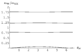
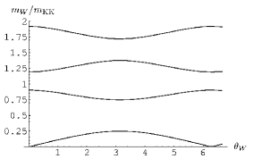
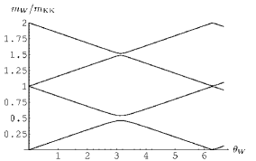
Figure 1: The masses of $W$ boson and its KK excited states are depicted in the unit of $m_{\rm KK}$ as functions of $\theta_{W}$ for $kR=12,1.2$, and $0.12$ from the left to the right.

5.2 The quark-lepton mass spectrum

The mass spectrum in the fermion sector depends on the bulk mass $M$ through $\alpha=(M/k)+\hbox{${1\over 2}$}$ in (5.1), which can be used to reproduce the mass spectrum of quarks and leptons. This is possible only in the warped spacetime, since the mass spectra for all fields are independent of $M$ in the flat case.

Before proceeding, we need to specify the fermion content in more detail. As a typical example we consider a model adopted in Ref. [11], in which

$$\begin{pmatrix}\nu_{e{\rm L}}&\tilde{\nu}_{e{\rm R}}\cr e_{\rm L}&\tilde{e}_{\rm R}\cr\tilde{e}_{\rm L}&e_{\rm R}\end{pmatrix}~{},~{}\begin{pmatrix}\tilde{\nu}_{e\rm L}&\nu_{e\rm R}\end{pmatrix}~{},~{}\begin{pmatrix}{d^{c}}_{{\rm L}}&\tilde{d^{c}}_{{\rm R}}\cr{u^{c}}_{\rm L}&\tilde{u^{c}}_{\rm R}\cr\tilde{u^{c}}_{\rm L}&{u^{c}}_{\rm R}\end{pmatrix}~{},~{}\begin{pmatrix}\tilde{d^{c}}_{\rm L}&{d^{c}}_{\rm R}\end{pmatrix}$$ (5.9)

are contained in the first generation. Boundary conditions are chosen such that only fields without tilde have zero modes for $\theta_{W}=0$. In our scheme the zero modes of $e$ and $u$ acquire nonvanishing masses when $\theta_{W}\not=0$.

The ratio of the lightest fermion mass $m_{f}(\alpha)$ to $m_{W}$ is almost independent of the value of $\theta_{W}$. For $z_{\pi}\gg 1$, in particular, it follows from (5.3) and (5.5) that

$$m_{f}(\alpha)\simeq\left(\frac{z_{\pi}\alpha(\alpha-1)k\pi R}{2\sinh(\alpha k\pi R)\sinh((\alpha-1)k\pi R)}\right)^{\frac{1}{2}}m_{W}~{}.$$ (5.10)

Fig. 2 shows the lightest mass $m_{0}$ determined from (5.1) as a function of $M/k$ at $\theta_{W}=\hbox{${1\over 2}$}\pi$. The fermion mass becomes the largest at $\alpha=\hbox{${1\over 2}$}$ ($M=0$). Its value is given by $m_{f}(\hbox{${1\over 2}$})=4.80\,m_{W}=386\,$GeV for $kR=12$ and $\theta_{W}=\hbox{${1\over 2}$}\pi$. Each $\lambda_{n}$ is an even function of $M$, as can be seen from (5.1) and (B.9). However, the corresponding mode functions are not invariant under $M\rightarrow-M$. (See Eq.(4.22).) $M/k$ is determined by the observed mass of quarks or leptons. The determined values of $M/k$ are listed in Table I. Since $\lambda_{n}$ are even functions of $M$, a given value of $\lambda_{n}$ in general corresponds to two values of $M/k$. Only one of them can be consistent with the observation as the other value leads to too large couplings to the KK excited states of the $W$ boson, which will be detailed in the next section.

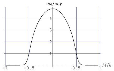
Figure 2: The lightest mass eigenvalue $m_{0}$ as a function of $M/k$ at $\theta_{W}=\hbox{${1\over 2}$}\pi$. The vertical axis is in the unit of $m_{W}$, or the fermion mass value at $M/k=\pm\frac{1}{2}$. $m_{0}/m_{W}$ has little dependence on $\theta_{W}$.

	$e$	$\mu$	$\tau$	$u$	$c$	$t$
mass (GeV)	5.11$\times 10^{-4}$	0.106	1.78	4$\times 10^{-3}$	1.3	175
$M/k$	0.865	0.715	0.633	0.81	0.64	0.436

Table I: The values of $M/k$ for leptons and quarks when $kR=12$ and $\theta_{W}=\hbox{${1\over 2}$}\pi$. The values have little dependence on $\theta_{W}$.

Notice that the values of the dimensionless parameter $M/k$ for all quarks and leptons fall in the range $(0.436\sim 0.865)$. Although there seems large hierarchy in the mass spectrum of order $m_{t}/m_{e}\sim 10^{5}$, there is no such hierarchy in terms of the dimensionless parameter $M/k$ which is more natural quantity in gauge theory in the RS spacetime. A similar role of the bulk mass in flat space has been pointed out in Ref.[33]. This might give an important hint in understanding the spectrum of quarks and leptons.

5.3 The mass and self-couplings of the Higgs boson

The 4D Higgs field whose VEV breaks the gauge symmetry $SU(2)\times U(1)$ to $U(1)_{\rm EM}$ is identified with the zero-mode $\varphi_{0}$ in $A^{7}_{z}$ in the present scheme. At the classical level, the potential for $\varphi_{0}$ is flat and $\varphi_{0}$ is massless. The flat direction is parametrized by the Wilson line phase $\theta_{W}$. At the quantum level the degeneracy is lifted, the effective potential $V_{\rm eff}(\theta_{W})$ becoming nontrivial. From the global minimum of $V_{\rm eff}(\theta_{W})$, the VEV of $\theta_{W}$ or $\varphi_{0}$ is determined. The Higgs field $\varphi_{0}$ acquires a nonvanishing finite mass. Although we do not explicitly calculate the effective potential in this paper, we can draw many important conclusions from the mass spectrum obtained in the preceeding sections.

The general argument given in Ref. [4] remains valid with minor changes resulting from the mass spectrum obtained in the preceeding sections. The one-loop effective potential $V_{\rm eff}(\theta_{W})$ in flat spacetime has been evaluated well [30, 21, 34, 31]. $V_{\rm eff}(\theta_{W})$ in the RS warped spacetime has been evaluated by Oda and Weiler[29]. At the one loop level it depends only on the mass spectrum of fields in the theory. Since the mass spectrum $\{m_{n}\}$ in the warped space is almost the same for large $n$ as that in flat space (see Eq.(5.8)), the resultant $V_{\rm eff}(\theta_{W})$ takes a similar form to that in the flat case[4]. It takes the form 

$$V_{\rm eff}(\theta_{W})=\frac{3}{128\pi^{6}}m_{\rm KK}^{4}f(\theta_{W}),$$ (5.11)

where $f(\theta_{W})$ is a dimensionless periodic function of $\theta_{W}$ with a period $2\pi$. The explicit form of $f(\theta_{W})$ depends on the matter content of the model, but its typical size is of order one in the minimal model or its minimal extension. When $V_{\rm eff}(\theta_{W})$ has a global minimum at a nontrivial $\theta_{W}=\theta_{W}^{\rm min}$, dynamical electroweak symmetry breaking takes place. The global minimum is located typically at $\theta_{W}^{\rm min}=(0.2\sim 1)\pi$ [16, 35]. It is possible to have a very small $\theta_{W}^{\rm min}\sim 0.01\pi$ by fine tuning of the matter content as shown in Ref. [14], but we will not consider such a case.

The Higgs mass $m_{H}$ is found by expanding $V_{\rm eff}(\theta_{W})$ around $\theta_{W}^{\rm min}$. More generally one obtains

$$V_{\rm eff}=\frac{3}{128\pi^{6}}m_{\rm KK}^{4}\sum_{n}{\displaystyle\phi^{n}\over\displaystyle n!}\bigg{\{}\frac{2\pi^{2}\alpha_{W}R(z_{\pi}^{2}-1)}{k}\bigg{\}}^{n/2}f^{(n)}(\theta_{W}^{\rm min})$$ (5.12)

where $\alpha_{W}\equiv g_{4}^{2}/4\pi$ and $f^{(n)}(\theta_{W})=d^{n}f(\theta_{W})/d\theta_{W}^{n}$. ($g_{4}\equiv g_{5}/\sqrt{\pi R}$ is the 4D weak $SU(2)_{L}$ gauge coupling constant before the symmetry breaking takes place. See the next section.) The Higgs mass is evaluated from the $n=2$ term;

$$m_{H}^{2}=f^{(2)}(\theta_{W}^{\rm min})\,\frac{3\alpha_{W}}{64\pi^{4}}\frac{R(z_{\pi}^{2}-1)}{k}\,m_{\rm KK}^{4}~{}~{},$$ (5.13)

Using Eqs.(5.4) and (5.5), one finds

$$m_{H}\!\!\! =\!\!\! \left\{f^{(2)}(\theta_{W}^{\rm min})\,\frac{3\alpha_{W}}{64\pi^{2}}\right\}^{\frac{1}{2}}\sqrt{kR}~{}m_{\rm KK}$$ (5.14)

$$=\!\!\! \left\{f^{(2)}(\theta_{W}^{\rm min})\,\frac{3\alpha_{W}}{32\pi}\right\}^{\frac{1}{2}}\frac{\pi kR}{2}{\displaystyle m_{W}\over\displaystyle\sin\hbox{${1\over 2}$}\theta_{W}^{\rm min}}~{}~{},$$ (5.15)

when $z_{\pi}\gg 1$. The important difference from the formula in flat space is the appearance of an enhancement factor $\hbox{${1\over 2}$}\pi kR\sim 18.8$. In the model of [16] it is found that $\big{\{}f^{(2)}(\theta_{W}^{\rm min})\big{\}}^{1/2}\sim 1.9$. With this value inserted $m_{H}$ is predicted to be 286 Gev or 125 GeV for $\theta_{W}^{\rm min}=0.2\pi$ or $0.5\pi$, respectively. It is remarkable that the predicted value is exactly in the range where experiments at LHC can explore.

The cubic and quartic coupling constants $\eta$ and $\lambda$ in the expansion $V_{\rm eff}=\hbox{${1\over 2}$}m_{H}^{2}\phi^{2}+\frac{1}{3}\eta\phi^{3}+\frac{1}{4}\lambda\phi^{4}+\cdots$ are given by

$$\hskip-28.45274pt\eta={\displaystyle 3\alpha_{W}^{3/2}m_{W}\over\displaystyle 32\pi^{1/2}\sin\hbox{${1\over 2}$}\theta_{W}}f^{(3)}(\theta_{W}^{\rm min})\bigg{(}\frac{\pi kR}{2}\bigg{)}^{2}~{}~{},$$ (5.16)

$$\hskip-28.45274pt\lambda={\displaystyle\alpha_{W}^{2}\over\displaystyle 16}f^{(4)}(\theta_{W}^{\rm min})\,\bigg{(}\frac{\pi kR}{2}\bigg{)}^{2}~{}~{}.$$ (5.17)

As in (5.15), there appears an enhancement factor $(\hbox{${1\over 2}$}\pi kR)^{2}$ for both $\eta$ and $\lambda$. In the standard model the relations $\eta=3\lambda v=3\lambda m_{W}/\sqrt{\pi\alpha_{W}}$ and $\lambda=m_{H}^{2}/2v^{2}=\pi m_{H}^{2}\alpha_{W}/2m_{W}^{2}$ hold at the tree level. In our scheme we find, instead, that

$$\hskip-28.45274pt\eta\cdot{\displaystyle\sqrt{\pi\alpha_{W}}\over\displaystyle 3\lambda m_{W}}={\displaystyle f^{(3)}(\theta_{W}^{\rm min})\over\displaystyle 2f^{(4)}(\theta_{W}^{\rm min})}{\displaystyle 1\over\displaystyle\sin\hbox{${1\over 2}$}\theta_{W}^{\rm min}}~{}~{},$$ (5.18)

$$\hskip-28.45274pt\lambda\cdot{\displaystyle 2m_{W}^{2}\over\displaystyle\pi m_{H}^{2}\alpha_{W}}={\displaystyle 4f^{(4)}(\theta_{W}^{\rm min})\over\displaystyle 3f^{(2)}(\theta_{W}^{\rm min})}\,\sin^{2}\hbox{${1\over 2}$}\theta_{W}^{\rm min}~{}~{}.$$ (5.19)

The behavior of these couplings in flat space has been investigated in Ref. [15].

5.4 $\theta_{W}\to 0$ limit

For the better understanding of the KK modes with respect to the broken $SU(2)\times U(1)$ gauge symmetry, we consider the $\theta_{W}\to 0$ limit. Take $(\psi_{2},\psi_{3})$ as an example. In this limit, the KK tower of $(\psi_{2},\psi_{3})$ splits into two KK towers of $\psi_{2}$ and $\psi_{3}$, and the $SU(2)\times U(1)$ gauge symmetry recovers. The mass spectrum determined from Eq.(5.1) splits into three cases.

1. $\lambda_{n}\to 0$

2. $F_{\alpha-1,\alpha-1}(\lambda_{n},z_{\pi})\to 0$

3. $F_{\alpha,\alpha}(\lambda_{n},z_{\pi})\to 0$

The case 1 corresponds to the zero modes ($n=0$) which are contained in the $Z_{2}$-even fields, i.e., $\psi_{{\rm L}2}$ and $\psi_{{\rm R}3}$. From (B.3),

$$F_{\alpha,\alpha}(\lambda_{0},z_{\pi}) \to -\frac{2\sinh(\alpha k\pi R)}{\pi\alpha}~{},$$

$$F_{\alpha,\alpha-1}(\lambda_{0},z_{\pi}) \to \frac{2z_{\pi}^{-\alpha}}{\pi\lambda_{0}}~{},$$

$$F_{\alpha-1,\alpha}(\lambda_{0},z_{\pi}) \to -\frac{2z_{\pi}^{\alpha-1}}{\pi\lambda_{0}}~{},$$ (5.20)

so that

$$\lambda_{0}=\left(\frac{\alpha(\alpha-1)}{z_{\pi}\sinh(\alpha k\pi R)\sinh((\alpha-1)k\pi R}\right)^{\frac{1}{2}}\frac{\theta_{W}}{2}+{\cal O}(\theta_{W}^{2}),$$ (5.21)

and the corresponding mode functions in (4.16) and (4.19) become

$$\tilde{f}^{+}_{2,0}(z)\!\!\! =\!\!\! {\cal O}(\theta_{W}),$$

$$\tilde{f}^{+}_{3,0}(z)\!\!\! =\!\!\! {\rm sgn}(\theta_{W})\left(\frac{2k\alpha}{z_{\pi}^{2\alpha}-1}\right)^{\frac{1}{2}}z^{\alpha-\frac{1}{2}},$$

$$\tilde{f}^{-}_{2,0}(z)\!\!\! =\!\!\! \left(\frac{2k(1-\alpha)}{z_{\pi}^{2(1-\alpha)}-1}\right)^{\frac{1}{2}}z^{\frac{1}{2}-\alpha}=\tilde{f}^{-}_{1,0}(z),$$

$$\tilde{f}^{-}_{3,0}(z)\!\!\! =\!\!\! {\cal O}(\theta_{W}).$$ (5.22)

In the case 2,

$$F_{\alpha-1,\alpha-1}(\lambda_{n},z_{\pi})=\frac{\theta_{W}^{2}}{\pi^{2}\lambda_{n}^{2}z_{\pi}F_{\alpha,\alpha}(\lambda_{n},z_{\pi})}+{\cal O}(\theta_{W}^{3}),$$ (5.23)

while $\lambda_{n}$, $F_{\alpha,\alpha}(\lambda_{n},z_{\pi})$, $F_{\alpha,\alpha-1}(\lambda_{n},z_{\pi})$ and $F_{\alpha-1,\alpha}(\lambda_{n},z_{\pi})$ remain finite. Thus the mode functions become

$$\tilde{f}^{+}_{2,n}(z)\!\!\! =\!\!\! \frac{\sqrt{k}\pi\lambda_{n}}{\sqrt{2}}\left\{\frac{Y_{\alpha-1}^{2}(\lambda_{n})}{Y_{\alpha-1}^{2}(\lambda_{n}z_{\pi})}-1\right\}^{-\frac{1}{2}}z^{\frac{1}{2}}F_{\alpha-1,\alpha-1}(\lambda_{n},z)=\tilde{f}^{+}_{1,n}(z),$$

$$\tilde{f}^{+}_{3,n}(z)\!\!\! =\!\!\! {\cal O}(\theta_{W}),$$

$$\tilde{f}^{-}_{2,n}(z)\!\!\! =\!\!\! \frac{\sqrt{k}\pi\lambda_{n}}{\sqrt{2}}\left\{\frac{Y_{\alpha-1}^{2}(\lambda_{n})}{Y_{\alpha-1}^{2}(\lambda_{n}z_{\pi})}-1\right\}^{-\frac{1}{2}}z^{\frac{1}{2}}F_{\alpha,\alpha-1}(\lambda_{n},z)=\tilde{f}^{-}_{1,n}(z),$$

$$\tilde{f}^{-}_{3,n}(z)\!\!\! =\!\!\! {\cal O}(\theta_{W}).$$ (5.24)

We observe that only $\psi_{2}$ components remain nonvanishing, which form $SU(2)$-doublets with $\psi_{1}$ components in this limit. In the case 3,

$$F_{\alpha,\alpha}(\lambda_{n},z_{\pi})=\frac{\theta_{W}^{2}}{\pi^{2}\lambda_{n}^{2}z_{\pi}F_{\alpha-1,\alpha-1}(\lambda_{n},z_{\pi})}+{\cal O}(\theta_{W}^{2}),$$ (5.25)

while $\lambda_{n}$, $F_{\alpha-1,\alpha-1}(\lambda_{n},z_{\pi})$, $F_{\alpha,\alpha-1}(\lambda_{n},z_{\pi})$ and $F_{\alpha-1,\alpha}(\lambda_{n},z_{\pi})$ remain finite. Thus the mode functions become

$$\tilde{f}^{+}_{2,n}(z)\!\!\! =\!\!\! {\cal O}(\theta_{W}),$$

$$\tilde{f}^{+}_{3,n}(z)\!\!\! =\!\!\! p_{\alpha,n}(\theta_{W})\frac{\sqrt{k}\pi\lambda_{n}}{\sqrt{2}}\left\{\frac{Y_{\alpha}^{2}(\lambda_{n})}{Y_{\alpha}^{2}(\lambda_{n}z_{\pi})}-1\right\}^{-\frac{1}{2}}z^{\frac{1}{2}}F_{\alpha-1,\alpha}(\lambda_{n},z),$$

$$\tilde{f}^{-}_{2,n}(z)\!\!\! =\!\!\! {\cal O}(\theta_{W}),$$

$$\tilde{f}^{-}_{3,n}(z)\!\!\! =\!\!\! p_{\alpha,n}(\theta_{W})\frac{\sqrt{k}\pi\lambda_{n}}{\sqrt{2}}\left\{\frac{Y_{\alpha}^{2}(\lambda_{n})}{Y_{\alpha}^{2}(\lambda_{n}z_{\pi})}-1\right\}^{-\frac{1}{2}}z^{\frac{1}{2}}F_{\alpha,\alpha}(\lambda_{n},z),$$ (5.26)

where $p_{\alpha,n}(\theta_{W})$ is defined by (B.6). Only $\psi_{3}$ components remain nonvanishing, forming $SU(2)$-singlets in this limit.

The cases 2 and 3 correspond to the non-zero modes. Their lightest modes have masses of order $m_{\rm KK}$ defined in (5.4). The solutions $\lambda_{n}$ of $F_{\alpha,\alpha}(\lambda_{n},z_{\pi})=0$ monotonically increase as $\left|\alpha\right|$ increases. Thus, if $\alpha>\frac{1}{2}$ ($\alpha<\frac{1}{2}$), the KK modes whose level number $n$ is odd (even) belong to the case 2, and the modes with even (odd) $n$ belong to the case 3. In the case of $\alpha=\frac{1}{2}$, i.e., $M=0$, the modes in the cases 2 and 3 are degenerate. In this case, all the Bessel functions appearing in mode functions reduce to trigonometric functions, and we can solve Eq.(5.1) analytically as

$$m_{n}=\left|n+\frac{1}{2}-\frac{\left|\pi-\theta_{W}\right|}{2\pi}\right|\,m_{\rm KK}\hskip 28.45274pt(0\leq\theta_{W}\leq 2\pi)$$ (5.27)

where $n=0,\pm 1,\pm 2,\cdots$. Here we have labeled the KK level number such that each KK mode is periodic in $\theta_{W}$. (See Sec. 5.1.)

It is convenient to divide the KK modes into three types classified above. In the case of the electron field ($\alpha=1.37$), for example, we denote each KK mode as

$$\tilde{\psi}_{{\rm L}2}(x,z)\!\!\! =\!\!\! \tilde{f}^{-}_{2,0}(z)e_{{\rm L}0}(x)+\sum_{n=1}^{\infty}\tilde{f}^{-}_{2,2n-1}(z)e_{{\rm L}n}(x)+\sum_{n=1}^{\infty}\tilde{f}^{-}_{2,2n}(z)\tilde{e}_{{\rm L}n}(x),$$

$$\tilde{\psi}_{{\rm L}3}(x,z)\!\!\! =\!\!\! \tilde{f}^{-}_{3,0}(z)e_{{\rm L}0}(x)+\sum_{n=1}^{\infty}\tilde{f}^{-}_{3,2n-1}(z)e_{{\rm L}n}(x)+\sum_{n=1}^{\infty}\tilde{f}^{-}_{3,2n}(z)\tilde{e}_{{\rm L}n}(x),$$

$$\tilde{\psi}_{{\rm R}2}(x,z)\!\!\! =\!\!\! \tilde{f}^{+}_{2,0}(z)e_{{\rm R}0}(x)+\sum_{n=1}^{\infty}\tilde{f}^{+}_{2,2n-1}(z)\tilde{e}_{{\rm R}n}(x)+\sum_{n=1}^{\infty}\tilde{f}^{+}_{2,2n}(z)e_{{\rm R}n}(x),$$

$$\tilde{\psi}_{{\rm R}3}(x,z)\!\!\! =\!\!\! \tilde{f}^{+}_{3,0}(z)e_{{\rm R}0}(x)+\sum_{n=1}^{\infty}\tilde{f}^{+}_{3,2n-1}(z)\tilde{e}_{{\rm R}n}(x)+\sum_{n=1}^{\infty}\tilde{f}^{+}_{3,2n}(z)e_{{\rm R}n}(x)~{}.$$ (5.28)

Similarly, the $W$ boson field ($\alpha=1$) is expanded as

$$\frac{1}{\sqrt{2}}\left(\tilde{A}^{1}_{\mu}+i\tilde{A}^{2}_{\mu}\right)\!\!\! =\!\!\! \tilde{h}^{1}_{A,0}(z)W_{\mu,0}(x)+\sum_{n=1}^{\infty}\tilde{h}^{1}_{A,2n-1}(z)W_{\mu,n}(x)+\sum_{n=1}^{\infty}\tilde{h}^{1}_{A,2n}(z)\tilde{W}_{\mu,n}(x),$$

$$\frac{1}{\sqrt{2}}\left(\tilde{A}^{4}_{\mu}+i\tilde{A}^{5}_{\mu}\right)\!\!\! =\!\!\! \tilde{h}^{4}_{A,0}(z)W_{\mu,0}(x)+\sum_{n=1}^{\infty}\tilde{h}^{4}_{A,2n-1}(z)W_{\mu,n}(x)+\sum_{n=1}^{\infty}\tilde{h}^{4}_{A,2n}(z)\tilde{W}_{\mu,n}(x).$$

In the expansions (5.28) and (LABEL:expansion4) a tower of 4D fields with tilde does not have a zero-mode at $\theta_{W}=0$.

6 Gauge couplings

One of the startling consequences in the dynamical gauge-Higgs unification in the RS spacetime is the prediction of non-universality of weak interctions in the fermion sector. With the wave functions of the gauge fields and quark-lepton fields being established, one can unambiguiously determine gauge couplings among them and their KK excited states from the observed quark and lepton masses. The relevant terms in the action are

$$I_{\rm gc}\!\!\! =\!\!\! \int d^{5}x\,\sqrt{-G}\,g_{5}\bar{\psi}\Gamma^{M}A_{M}\psi$$ (6.1)

$$=\!\!\! \int d^{4}x\int_{1}^{z_{\pi}}\frac{dz}{k}\,g_{5}\,\Big{\{}\bar{\tilde{\psi}}\gamma^{\mu}\tilde{A}_{\mu}\tilde{\psi}+\cdots\Big{\}}~{}~{}.$$ (6.2)

Inserting (5.28) and (LABEL:expansion4) into (6.2), one obtains

$${\cal L}^{(4)}_{\rm gc}=\sum_{n}\frac{g_{(n)}}{\sqrt{2}}\left(\bar{e}_{{\rm L}0}\gamma^{\mu}W_{\mu,n}\nu_{{\rm L}0}+{\rm h.c.}\right)+\cdots~{},$$ (6.3)

where the ellipsis denotes terms involving the KK modes of the fermions or $\tilde{W}_{\mu,n}$. Here the 4D gauge coupling constants are given by

$$g_{(0)}(\theta_{W},\alpha)\!\!\! \equiv\!\!\! g_{5}\int_{1}^{z_{\pi}}\frac{dz}{k}\left(\tilde{f}^{-}_{2,0}\tilde{h}^{1}_{A,0}+\tilde{f}^{-}_{3,0}\tilde{h}^{4}_{A,0}\right)\tilde{f}^{-}_{1,0}~{}~{},$$

$$g_{(n)}(\theta_{W},\alpha)\!\!\! \equiv\!\!\! g_{5}\int_{1}^{z_{\pi}}\frac{dz}{k}\left(\tilde{f}^{-}_{2,0}\tilde{h}^{1}_{A,2n-1}+\tilde{f}^{-}_{3,0}\tilde{h}^{4}_{A,2n-1}\right)\tilde{f}^{-}_{1,0}\hskip 14.22636pt(n\geq 1)~{},$$ (6.4)

which depend on $\theta_{W}$ and $\alpha=(M/k)+\hbox{${1\over 2}$}$.

Consider the 4D weak gauge coupling $g_{(0)}$. In the $\theta_{W}\to 0$ limit the electroweak symmetry remains unbroken so that $g_{(0)}$ must be universal for all quarks and leptons. Indeed, the mode functions of 4D gauge fields are constants

$$\tilde{h}^{1}_{A,0}(z)\Big{|}_{\theta_{W}=0}=\frac{1}{\sqrt{\pi R}}~{}~{},~{}~{}\tilde{h}^{4}_{A,0}(z)\Big{|}_{\theta_{W}=0}=0~{}~{},$$ (6.5)

and $\tilde{f}^{-}_{2,0}(z)\big{|}_{\theta_{W}=0}$ coincides with $\tilde{f}^{-}_{1,0}(z)$ (see Eq. (5.22)) so that

$$g_{(0)}(\theta_{W}=0,\alpha)=g_{5}\int_{1}^{z_{\pi}}\frac{dz}{k}\frac{1}{\sqrt{\pi R}}\left(\tilde{f}^{-}_{1,0}\right)^{2}=\frac{g_{5}}{\sqrt{\pi R}}\equiv g_{4}$$ (6.6)

where the normalization condition (4.13) has been used. $g_{4}$ is the 4D $SU(2)_{L}$ gauge coupling constant in the unbroken theory. It is seen that $g_{(0)}$ is independent of $\alpha$, or the fermion bulk mass $M$, at $\theta_{W}=0$.

When the electroweak symmetry breaking takes place so that $\theta_{W}\not=0$, the overlap integral in (6.4) has nontrivial dependence on $\alpha$. It leads to the violation of the universality in the couplings of the charged current to the $W$ boson. In Table II, $g_{(0)}/g_{4}$ is tabulated for electrons for various values of $\theta_{W}$. The deviation of $g_{(0)}^{\rm electron}$ from $g_{4}$ remains very small.

$\theta_{W}$	$g_{(0)}^{\rm electron}/g_{4}$
0	1
$0.2\pi$	1.00092
$0.5\pi$	1.00489
$\pi$	1.00999

Table II: $g_{(0)}/g_{4}$ for electrons when $kR=12$.

The dependence of $g_{(0)}/g_{4}$ on the fermion mass, or on $M/k$, is depicted in Fig. 3. It shows that $g_{(0)}$ is almost constant for $\left|M\right|/k>\frac{1}{2}$. This feature is understood from the profiles of the mode functions. For $M/k>\frac{1}{2}$ ($\alpha>1$),

$$\tilde{f}^{-}_{2,0}(z) \simeq \tilde{f}^{-}_{1,0}(z)\simeq\sqrt{2k(\alpha-1)}z^{\frac{1}{2}-\alpha},$$

$$\tilde{f}^{-}_{3,0}(z) \simeq \sqrt{\frac{k(\alpha-1)}{2}}\frac{\sin\theta_{W}}{z_{\pi}^{2\alpha}}z^{\frac{1}{2}+\alpha},$$ (6.7)

and for $M/k<-\frac{1}{2}$ ($\alpha<0$),

$$\tilde{f}^{-}_{2,0}(z) \simeq \left|\cos\frac{\theta_{W}}{2}\right|\tilde{f}^{-}_{1,0}(z)\simeq\left|\cos\frac{\theta_{W}}{2}\right|\frac{\sqrt{2k(1-\alpha)}}{z_{\pi}^{1-\alpha}}z^{\frac{1}{2}-\alpha},$$

$$\tilde{f}^{-}_{3,0}(z) \simeq p_{0}\sin\frac{\theta_{W}}{2}\tilde{f}^{-}_{1,0}(z)\simeq p_{0}\sin\frac{\theta_{W}}{2}\frac{\sqrt{2k(1-\alpha)}}{z_{\pi}^{1-\alpha}}z^{\frac{1}{2}-\alpha},$$ (6.8)

where $p_{0}\equiv{\rm sgn}(\cos\frac{1}{2}\theta_{W})$. Here we have made use of the fact that the eigenvalue $\lambda_{0}$ is exponentially small for $\left|M\right|/k>\frac{1}{2}$ (see Fig. 2) and Eq.(B.3). For $M/k>\frac{1}{2}$, we can see from Eq.(6.7) that the first terms in Eq.(6.4) dominate and $\tilde{f}^{-}_{1,0}(z)\tilde{f}^{-}_{2,0}(z)/k$ plays a role similar to that of the delta function $\delta(z-1)$ since it is strongly localized around $z=1$. For $M/k<-\frac{1}{2}$, all fermion mode functions in Eq.(6.4) are dominant around $z=z_{\pi}$, thus picking up the value of $\tilde{h}^{1,4}_{A,0}(z)$ in the vicinity of $z=z_{\pi}$. As a consequence the gauge coupling $g_{(0)}$ is almost independent of $\alpha$ for $\left|M\right|/k>\frac{1}{2}$. The asymptotic values of $g_{(0)}$ in this region is evaluated by the following behavior of the mode functions for the gauge fields.

$$\tilde{h}^{1}_{A,0}(1) \simeq \frac{1}{\sqrt{\pi R}},$$

$$\frac{\tilde{h}^{1}_{A,0}(z_{\pi})}{\tilde{h}^{1}_{A,0}(1)} \simeq \cos^{2}\frac{\theta_{W}}{2},\;\;\;\;\;\frac{\tilde{h}^{4}_{A,0}(z_{\pi})}{\tilde{h}^{1}_{A,0}(1)}\simeq\sin\frac{\theta_{W}}{2}\cos\frac{\theta_{W}}{2}.$$ (6.9)

Here we have used Eq.(5.5). Using these relations, $g_{(0)}$ is evaluated to be

$$g_{(0)}\left(\frac{M}{k}>\frac{1}{2}\right) \simeq g_{4}~{}~{},$$

$$g_{(0)}\left(\frac{M}{k}<-\frac{1}{2}\right) \simeq g_{4}\Big{|}\cos\frac{\theta_{W}}{2}\Big{|}~{}~{}.$$ (6.10)

There arise small corrections to the asymptotic values above due to the extended nature of the fermion mode functions.

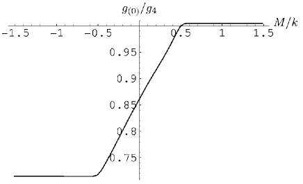
Figure 3: The 4D gauge coupling $g_{(0)}/g_{4}$ as a function of $M/k$ for $\theta_{W}=\hbox{${1\over 2}$}\pi$ and $kR=12$.

In view of stringent experimental constraints on the gauge coupling universality, we need to examine precisely how much deviation from the universality results. For quarks and leptons with the values of $M/k$ in Table I, the couplings to the $W$ boson $g_{(0)}$ are evaluated from (6.4). The quantity of physical interest is the degree of the violation of the universality. Therefore, for each quark or lepton, $g_{(0)}/g_{(0)}^{\rm electron}-1$ is tabulated in Table III. It is seen that the violation of the universality in the weak gauge coupling is within the current experimental bounds. Violation of the universality becomes larger for heavy fermions.

$\theta_{W}$	$\mu$(muon)	$\tau$(tau)	$t$(top)
$0.2\pi$	$-1.74\times 10^{-9}$	$-4.69\times 10^{-7}$	$-4.3\times 10^{-3}$
$0.5\pi$	$-9.26\times 10^{-9}$	$-2.50\times 10^{-6}$	$-2.2\times 10^{-2}$
$0.8\pi$	$-1.70\times 10^{-8}$	$-4.60\times 10^{-6}$	$-4.0\times 10^{-2}$

Table III: Non-universality of weak interactions. The deviation of $g_{(0)}^{\rm f}/g_{(0)}^{\rm electron}$ from 1 for f$\,=\mu,\tau,t$ is listed. ($kR=12$.)

Next, we consider the couplings to the KK excited states of $W$ boson, $g_{(n)}$. In Fig. 4, $g_{(n)}/g_{4}$ ($n=1,2,3$) are shown as functions of $M/k$ at $\theta_{W}=\hbox{${1\over 2}$}\pi$. These quantities at $\theta_{W}=0$ have been evaluated by Gherghetta and Pomarol[27]. Qualitative behavior does not change for $\theta_{W}\not=0$.

Since for $M/k=\frac{1}{2}$ ($\alpha=1$)

$$z^{\frac{1}{2}}\tilde{f}^{-}_{1,n}(z)\!\!\! =\!\!\! \frac{1}{\sqrt{\pi R}}~{},$$ (6.11)

$$z^{\frac{1}{2}}\tilde{f}^{-}_{2,n}(z)\!\!\! =\!\!\! \tilde{h}^{1}_{A,n}(z)~{},$$ (6.12)

$$z^{\frac{1}{2}}\tilde{f}^{-}_{3,n}(z)\!\!\! =\!\!\! \tilde{h}^{4}_{A,n}(z)~{},$$ (6.13)

it follows with the normalization condition in (3.52) that the 4D gauge couplings satisfy

$$g_{(0)}(\theta_{W},1)=g_{4}~{}~{},~{}~{}g_{(n)}(\theta_{W},1)=0~{}~{}.$$ (6.14)

In the $\theta_{W}\rightarrow 0$ limit, this feature has been explained in Ref. [27] as a result of the accidental conformal symmetry or the translational invariance along the fifth direction. We have seen that the relation (6.14) holds even in the case $\theta_{W}\neq 0$ where such accidental symmetry no longer exists.

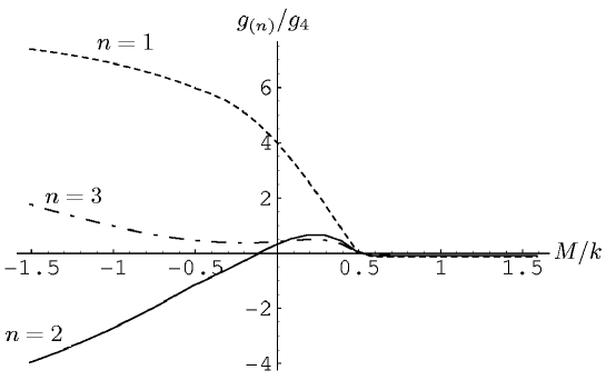
Figure 4: The gauge couplings to the $n$-th KK excited states of $W$, $g_{(n)}$ ($n=1,2,3$) as functions of $M/k$ at $\theta_{W}=\hbox{${1\over 2}$}\pi$.

As mentioned in the derivation of (6.10), the fermion mode functions are strongly localized at the boundary $z=1$ when $M/k>\frac{1}{2}$. Due to this property, $g_{(n)}$ ($n\geq 1$) are almost independent of $\alpha$ for $M/k>\frac{1}{2}$ just like $g_{(0)}$. On the other hand, they still have nontrivial $\alpha$-dependences around $M/k\simeq-1$ in Fig. 4. This is because $\tilde{h}_{A,n}^{1,4}(z)$ ($n\geq 1$) oscillate around $z=z_{\pi}$ where the fermion mode functions are dominant. It has been argued in Ref. [26] that brane fermions have universal coupling $\left|g_{(n)}\right|/g_{4}=\sqrt{2k\pi R}$. We have numerically confirmed that $\left|g_{(n)}\right|/g_{4}$ ($n=1,2,3$) in Fig. 4 approach the asymptotic value $\sqrt{2k\pi R}\simeq 8.68$ as $M/k\rightarrow-\infty$.

We note that a given value of $\lambda_{n}$ determines only the absolute value of $M/k$ while its sign remains undetermined. (See Fig. 2.) The values of $M/k$ in Table I are the only values consistent with experiments, as fermions with the values of the opposite sign have too large $g_{(n)}$ leading to contradiction to precision measurements as discussed by Chang et al[26]. The couplings $g_{(1)}/g_{4}$, $g_{(2)}/g_{4}$, and $g_{(3)}/g_{4}$ approach $-0.13$, $-0.090$, and $-0.073$ for $M/k>0.6$, respectively.

7 Yukawa couplings

The Yukawa couplings in four dimensions originate from five-dimensional gauge interactions in the dynamical gauge-Higgs unification scheme. From the 5D interaction

$${\cal L}_{\rm yukawa}\!\!\! =\!\!\! \sqrt{-G}g_{5}\bar{\psi}\Gamma^{4}A_{z}\psi$$ (7.1)

$$=\!\!\! g_{5}(\bar{\tilde{\psi}}_{1},\bar{\tilde{\psi}}_{2},\bar{\tilde{\psi}}_{3})\gamma_{5}\frac{1}{2}\left(\begin{array}[]{ccc}&&\\ &&-i\tilde{A}^{7}_{z}\\ &i\tilde{A}^{7}_{z}&\end{array}\right)\left(\begin{array}[]{c}\tilde{\psi}_{1}\\ \tilde{\psi}_{2}\\ \tilde{\psi}_{3}\end{array}\right)$$ (7.8)

the 4D coupling

$${\cal L}^{(4)}_{\rm yukawa}=-iy_{e}\varphi_{0}\bar{e}_{{\rm L}0}e_{{\rm R}0}+{\rm h.c.}$$ (7.9)

emerges. Here the Yukawa coupling constant $y_{e}$ is given by

$$y_{e}\equiv\frac{g_{5}}{2}\int_{1}^{z_{\pi}}\!\!dz\;\tilde{h}^{7}_{\varphi,0}\left(\tilde{f}^{-}_{2,0}\tilde{f}^{+}_{3,0}-\tilde{f}^{-}_{3,0}\tilde{f}^{+}_{2,0}\right),$$ (7.10)

where

$$\tilde{h}^{7}_{\varphi,0}(z)=\sqrt{\frac{2}{k(z_{\pi}^{2}-1)}}~{}z.$$ (7.11)

In accordance with the standard model, we define the “Higgs VEV” $v$ by

$$v\equiv\frac{2m_{W}}{g_{4}}\sim 246\,{\rm GeV}~{}.$$ (7.12)

$g_{4}$ is defined in Eq.(6.6). In the standard model, the fermion mass, say, the electron mass $m_{e}$ is related to $v$ and $y_{e}$ by $m_{e}=\left|y_{e}\right|v$. Hence we define

$$r\equiv\frac{2\left|y_{e}\right|m_{W}}{g_{4}m_{e}}~{},$$ (7.13)

which equals one for all fermions in the standard model. In the present scheme, this ratio $r$ is not a constant but has a distinct value for each fermion. In Fig. 5, we plot $r$ as a function of $M/k$.

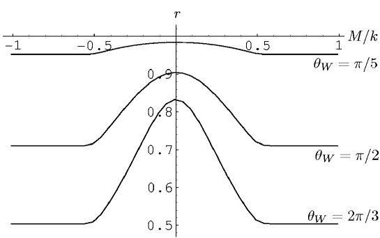
Figure 5: The ratio $r$ defined in Eq.(7.13) as a function of $M/k$. $\theta_{W}=\frac{1}{5}\pi,\hbox{${1\over 2}$}\pi,\frac{2}{3}\pi$. Significant reduction of the Yukawa couplings is seen. The asymptotic value of $r$ for $|M/k|\gg\hbox{${1\over 2}$}$ is $|\cos\hbox{${1\over 2}$}\theta_{W}|$.

Note that $r$ is an even function of $M/k$ as $y_{e}$ is even under $M\leftrightarrow-M$. (See Eq.(4.22).) For $M=0$, all the Bessel functions appearing in the mode functions reduce to trigonometric functions, and we can analytically calculate $r$ as

$$r(0)\simeq\frac{2}{\theta_{W}}\sin\frac{\theta_{W}}{2},$$ (7.14)

for $-\pi\leq\theta_{W}\leq\pi$. The approximate expression of $m_{W}$ (5.5) has been made use of. For $\left|M\right|/k>\frac{1}{2}$, $r$ is almost independent of $M/k$. From Eqs.(6.7), (6.8) and (4.22), the asymptotic constant value is evaluated to be

$$r\left(\frac{\left|M\right|}{k}>\frac{1}{2}\right)\simeq\left|\cos\frac{\theta_{W}}{2}\right|~{}.$$ (7.15)

This is a stringent result. As $\theta_{W}$ approaches $\pi$, the asymptotic value of $r$, namely the Yukawa coupling, vanishes. The significant reduction in the Yukawa couplings result for all quarks and leptons for $|\theta_{W}|>0.3\pi$. The measurement of the Yukawa couplings definitely sheds light on the origin of the Higgs field.

8 Conclusion and discussions

In the present paper we have shown that many intriguing phenomenological consequences follow in the quark-lepton sector in the scheme of the dynamical gauge-Higgs unification in the RS warped spacetime. The 4D Higgs field is identified with the extra-dimensional component of the gauge potentials, representing fluctuations of the Wilson line phase $\theta_{W}$. Dynamical electroweak symmetry breaking takes place when the phase $\theta_{W}$ takes a nontrivial value by quantum effects.

Another important quantity for discussing fermion phenomenology is the bulk mass $M$. The dimensionless parameter $c\equiv M/k$, where $-k^{2}$ is the AdS curvature in the bulk, becomes crucial for controling the wave functions of quarks and leptons. When $\theta_{W}=0$, quarks and leptons remain massless irrespective of the value of $c$ although their wave functions depend on $c$. As $\theta_{W}\not=0$ and the dynamical electroweak symmetry breaking is induced, quarks and leptons acquire nonvanishing masses, $m_{f}$, which depend on both $\theta_{W}$ and $c$. Remarkably $m_{f}/m_{W}$ has little dependence on $\theta_{W}$ so that the parameter $c$ is unambiguiously determined by the observed quark and lepton masses. The values of $c$ are 0.865 and 0.436 for electrons and top quarks, respectively. Although there is huge hierarchy in the fermion masses, there does not appear such hierarchic structure in $c$, the more natural entity in the RS spacetime.

With the value of $c$ fixed for each fermion, one can make important predictions for the gauge and Yukawa couplings of quarks and leptons. First, non-universality in the weak interactions results for the couplings of quarks and leptons to the $W$ boson. The magnitude of the non-universality is, however, very tiny. We have found that the violation of the universality for $\theta_{W}=\hbox{${1\over 2}$}\pi$ is of magnitudes of $9.26\times 10^{-9}$, $2.50\times 10^{-6}$, and $2.2\times 10^{-2}$ for $\mu$-$e$, $\tau$-$e$, and $t$-$e$, respectively. These numbers are well within the current experimental limits. Improvement of experiments is necessary to confirm the non-universality of the weak interactions.

Secondly, the Yukawa coupling of quarks and leptons to the 4D Higgs field suffers from large corrections. Compared with the Yukawa coupling in the standard model, the Yukawa coupling in the dynamical gauge-Higgs unification is suppressed by a factor $\sim|\cos\hbox{${1\over 2}$}\theta_{W}|$. This effect is observable at LHC, should the direct Yukawa coupling be measured.

The non-universality of the weak interactions and the reduction of the Yukawa coupling are the two major predictions we obtained in the present paper. As mentioned in the introduction, the scenario of the dynamical gauge-Higgs unification is by no means complete in the current form, however. The non-universality of the weak interactions is expected for neutral currents as well. To tackle this problem definitively, however, one first needs to improve the model so as to have the correct value for the Weinberg angle. The improvement along this direction is important considering that constraints on the non-universality of the couplings to the $Z$ boson are much severer than those for the $W$ boson discussed in this paper[36]. One model with the correct value for the Weinberg angle has been provided in Ref. [3], for which it is desired to perform analysis outlined in the present paper. Secondly, right-handed components of fermions are dominantly localized near the TeV brane at $z=z_{\pi}$ so that they are expected to have too large couplings to the Kaluza-Klein excited states of neutral gauge bosons, which may contradicts with the current precision measurements. Additional structure might be required to obtain a realistic model. Thirdly, neutrinos and down-type quarks, in the present minimal model, remain massless. The origin of masses of those fermions need to be clarified. Fourthly, in the pure gauge interactions it seems very difficult to accommodate CP violation as stressed by Frere[37]. The third and fourth problems may suggest the existence of a fundamental scalar field. Further, implications to the $S$, $T$ parameters and the unitarity need to be investigated. We shall come back to these issues in the near future.

Acknowledgments

We would like to thank S. Kanemura for many enlightening comments. This work was supported in part by Scientific Grants from the Ministry of Education and Science, Grant No. 17540257, Grant No. 17043007, Grant No. 13135215, and Grant No. 15340078 (Y.H), and by JSPS fellowship No. 0509241 (Y.S.)

Appendix A Useful formulae for Bessel functions

In this appendix we collect useful formulae for the Bessel functions frequently used in the text. $J_{\alpha}(z)$ and $Y_{\alpha}(z)$ denote the Bessel functions of the first and second kinds, respectively. For $z\ll 1$,

$$J_{\alpha}(z)=\frac{1}{\Gamma(\alpha+1)}\left(\frac{z}{2}\right)^{\alpha}\left\{1+{\cal O}(z^{2})\right\}~{}.$$ (A.1)

$Y_{\alpha}(z)$ is defined as

$$Y_{\alpha}(z)\equiv\begin{cases}{\displaystyle 1\over\displaystyle\sin\pi\alpha}\left\{\cos\pi\alpha\cdot J_{\alpha}(z)-J_{-\alpha}(z)\right\}&\hbox{for }\alpha\not=\hbox{ an integer,}\cr\kern 10.0pt\cr{\displaystyle 1\over\displaystyle\pi}\left[{\displaystyle\partial J_{\alpha}(z)\over\displaystyle\partial\alpha}-(-1)^{n}{\displaystyle\partial J_{-\alpha}(z)\over\displaystyle\partial\alpha}\right]_{\alpha=n}&\hbox{for }\alpha=n=\hbox{ an integer.}\end{cases}$$ (A.2)

Their behavior for $\left|z\right|\gg 1$ is given by

$$J_{\alpha}(z) \sim \sqrt{\frac{2}{\pi z}}\cos\left(z-\frac{(2\alpha+1)\pi}{4}\right),$$

$$Y_{\alpha}(z) \sim \sqrt{\frac{2}{\pi z}}\sin\left(z-\frac{(2\alpha+1)\pi}{4}\right).$$ (A.3)

These Bessel functions $Z_{\alpha}(z)=J_{\alpha}(z)$ or $Y_{\alpha}(z)$ satisfy

$$Z_{\alpha-1}(z)+Z_{\alpha+1}(z)\!\!\! =\!\!\! \frac{2\alpha}{z}Z_{\alpha}(z),$$

$$\frac{dZ_{\alpha}(z)}{dz}=\frac{\alpha}{z}Z_{\alpha}(z)-Z_{\alpha+1}(z)\!\!\! =\!\!\! Z_{\alpha-1}(z)-\frac{\alpha}{z}Z_{\alpha}(z),$$

$$J_{\alpha}(z)Y_{\alpha-1}(z)-Y_{\alpha}(z)J_{\alpha-1}(z)\!\!\! =\!\!\! \frac{2}{\pi z}.$$ (A.4)

The following integral formula is useful for determining normalization factors of mode functions.

$$\int^{z}\!\!dz\;zZ_{\alpha}(\lambda z)\tilde{Z}_{\alpha}(\lambda z)\!\!\! =\!\!\! \frac{z^{2}}{4}\left\{2Z_{\alpha}(\lambda z)\tilde{Z}_{\alpha}(\lambda z)-Z_{\alpha-1}(\lambda z)\tilde{Z}_{\alpha+1}(\lambda z)-Z_{\alpha+1}(\lambda z)\tilde{Z}_{\alpha-1}(\lambda z)\right\},$$

where $Z_{\alpha}(z)$, $\tilde{Z}_{\alpha}(z)$ are linear combinations of $J_{\alpha}(z)$ and $Y_{\alpha}(z)$. Besides the Bessel functions, the following formula is also useful.

$$\Gamma(\alpha)\Gamma(1-\alpha)=\frac{\pi}{\sin\pi\alpha}~{}~{}.$$ (A.6)

Appendix B Definition of various functions

We define

$$F_{\alpha,\beta}(\lambda,z)\equiv Y_{\beta}(\lambda)J_{\alpha}(\lambda z)-J_{\beta}(\lambda)Y_{\alpha}(\lambda z)~{}.$$ (B.1)

With the aid of the third equation in (A.4), it satisfies the relation,

$$F_{\alpha-1,\alpha}(\lambda,z)F_{\alpha,\alpha-1}(\lambda,z)=F_{\alpha-1,\alpha-1}(\lambda,z)F_{\alpha,\alpha}(\lambda,z)-\frac{4}{\pi^{2}\lambda^{2}z}.$$ (B.2)

For $\lambda,\lambda z\ll 1$,

$$F_{\alpha,\alpha}(\lambda,z) \to -\frac{z^{\alpha}-z^{-\alpha}}{\pi\alpha}~{},$$

$$F_{\alpha,\alpha-1}(\lambda,z) \to \frac{2z^{-\alpha}}{\pi\lambda}-\frac{\lambda z^{\alpha}}{2\pi\alpha(\alpha-1)}~{},$$

$$F_{\alpha-1,\alpha}(\lambda,z) \to -\frac{2z^{\alpha-1}}{\pi\lambda}+\frac{\lambda z^{-\alpha+1}}{2\pi\alpha(\alpha-1)}~{}.$$ (B.3)

From these functions, the coefficients in the normalized mode functions are written as

$$C^{\rm d}_{\alpha,n}(\theta_{W})\!\!\! \equiv\!\!\! \frac{\sqrt{2k}}{z_{\pi}}\left\{\frac{F_{\alpha-1,\alpha-1}^{2}}{\sin^{2}\hbox{${1\over 2}$}\theta_{W}}+\frac{F_{\alpha,\alpha-1}^{2}}{\cos^{2}\hbox{${1\over 2}$}\theta_{W}}-\frac{\pi^{2}\lambda_{n}^{2}}{\sin^{2}\theta_{W}}F^{2}_{\alpha-1,\alpha-1}F^{2}_{\alpha,\alpha-1}-\frac{4}{\pi^{2}\lambda_{n}^{2}z_{\pi}^{2}}\right\}^{-\frac{1}{2}},$$ (B.4)

$$C^{\rm s}_{\alpha,n}(\theta_{W})\!\!\! \equiv\!\!\! -\cot\frac{\theta_{W}}{2}\cdot\frac{F_{\alpha-1,\alpha-1}}{F_{\alpha-1,\alpha}}\cdot C^{\rm d}_{\alpha,n}(\theta_{W})=\tan\frac{\theta_{W}}{2}\cdot\frac{F_{\alpha,\alpha-1}}{F_{\alpha,\alpha}}\cdot C^{\rm d}_{\alpha,n}(\theta_{W}),$$ (B.5)

where $\lambda_{n}$ is a solution of Eq.(5.1), and the arguments of all $F_{\alpha,\beta}$ in the definition of $C^{\rm d,s}_{\alpha,n}$ are $(\lambda_{n},z_{\pi})$. In the second equation, we have used Eqs.(5.1) and (5.2). Using the sign factors $p_{\alpha,n}(\theta_{W})=\pm 1$ defined by

$$p_{\alpha,n}(\theta_{W})\equiv{\rm sgn}\left(-\cot\frac{\theta_{W}}{2}\cdot\frac{F_{\alpha-1,\alpha-1}(\lambda_{n},z_{\pi})}{F_{\alpha-1,\alpha}(\lambda_{n},z_{\pi})}\right)={\rm sgn}\left(\tan\frac{\theta_{W}}{2}\cdot\frac{F_{\alpha,\alpha-1}(\lambda_{n},z_{\pi})}{F_{\alpha,\alpha}(\lambda_{n},z_{\pi})}\right),$$ (B.6)

$C^{\rm s}_{\alpha,n}(\theta_{W})$ can be rewritten as

$$C^{\rm s}_{\alpha,n}(\theta_{W})=p_{\alpha,n}(\theta_{W})\frac{\sqrt{2k}}{z_{\pi}}\left\{\frac{F_{\alpha,\alpha}^{2}}{\sin^{2}\hbox{${1\over 2}$}\theta_{W}}+\frac{F_{\alpha-1,\alpha}^{2}}{\cos^{2}\hbox{${1\over 2}$}\theta_{W}}-\frac{\pi^{2}\lambda_{n}^{2}}{\sin^{2}\theta_{W}}F^{2}_{\alpha,\alpha}F^{2}_{\alpha-1,\alpha}-\frac{4}{\pi^{2}\lambda_{n}^{2}z_{\pi}^{2}}\right\}^{-\frac{1}{2}},$$ (B.7)

where the arguments of $F_{\alpha,\beta}$ are $(\lambda_{n},z_{\pi})$.

One can express $F_{\alpha,\alpha}(\lambda,z)$, $F_{\alpha,\alpha-1}(\lambda,z)$ and $F_{\alpha-1,\alpha}(\lambda,z)$ solely in terms of the Bessel function of the first kind;

$$F_{\alpha,\alpha}(\lambda,z)\!\!\! =\!\!\! -\frac{1}{\sin\pi\alpha}\left\{J_{-\alpha}(\lambda)J_{\alpha}(\lambda z)-J_{\alpha}(\lambda)J_{-\alpha}(\lambda z)\right\},$$

$$F_{\alpha,\alpha-1}(\lambda,z)\!\!\! =\!\!\! \frac{1}{\sin\pi\alpha}\left\{J_{1-\alpha}(\lambda)J_{\alpha}(\lambda z)+J_{\alpha-1}(\lambda)J_{-\alpha}(\lambda z)\right\},$$

$$F_{\alpha-1,\alpha}(\lambda,z)\!\!\! =\!\!\! -\frac{1}{\sin\pi\alpha}\left\{J_{-\alpha}(\lambda)J_{\alpha-1}(\lambda z)+J_{\alpha}(\lambda)J_{1-\alpha}(\lambda z)\right\}.$$ (B.8)

The first equation demonstrates that $F_{\alpha,\alpha}(\lambda,z)=F_{-\alpha,-\alpha}(\lambda,z)$. From (B.8), we can see that under the exchange $\alpha\leftrightarrow 1-\alpha$,

$$F_{\alpha,\alpha}(\lambda,z) \leftrightarrow F_{1-\alpha,1-\alpha}(\lambda,z)=F_{\alpha-1,\alpha-1}(\lambda,z)~{},$$

$$F_{\alpha,\alpha-1}(\lambda,z) \leftrightarrow -F_{\alpha-1,\alpha}(\lambda,z)~{}.$$ (B.9)

It follows from Eqs.(B.5) and (B.7) that

$$C^{\rm d}_{\alpha,n}(\theta_{W})\leftrightarrow p_{\alpha,n}(\theta_{W})C^{\rm s}_{\alpha,n}(\theta_{W})~{}.$$ (B.10)

References

-
[1]
- [2] R. Contino, Y. Nomura and A. Pomarol, Nucl. Phys. B671 (2003) 148.
- [3] K. Agashe, R. Contino and A. Pomarol, Nucl. Phys. B719 (2005) 165; K. Agashe and R. Contino, hep-ph/0510164.
- [4] Y. Hosotani and M. Mabe, Phys. Lett. B615 (2005) 257;
- [5] D.B. Fairlie, Phys. Lett. B82 (1979) 97; J. Phys. G5 (1979) L55.
- [6] N. Manton, Nucl. Phys. B158 (1979) 141; P. Forgacs and N. Manton, Comm. Math. Phys. 72 (1980) 15.
- [7] Y. Hosotani, Phys. Lett. B126 (1983) 309; Phys. Lett. B129 (1984) 193; Phys. Rev. D29 (1984) 731.
- [8] Y. Hosotani, Ann. Phys. (N.Y.) 190 (1989) 233.
- [9] H. Hatanaka, T. Inami and C.S. Lim, Mod. Phys. Lett. A13 (1998) 2601.
- [10] A. Pomarol and M. Quiros, Phys. Lett. B438 (1998) 255; I. Antoniadis, Phys. Lett. B246 (1990) 377.
- [11] I. Antoniadis, K. Benakli and M. Quiros, New. J. Phys.3 (2001) 20.
- [12] C. Csaki, C. Grojean and H. Murayama, Phys. Rev. D67 (2003) 085012; C.A. Scrucca, M. Serone and L. Silverstrini, Nucl. Phys. B669 (2003) 128.
- [13] L.J. Hall, Y. Nomura and D. Smith, Nucl. Phys. B639 (2002) 307; L. Hall, H. Murayama, and Y. Nomura, Nucl. Phys. B645 (2002) 85; G. Burdman and Y. Nomura, Nucl. Phys. B656 (2003) 3; I. Gogoladze, Y. Mimura and S. Nandi, Phys. Rev. Lett. 91 (2003) 141801; C.A. Scrucca, M. Serone, L. Silvestrini and A. Wulzer, JHEP 0402 (2004) 49; G. Panico and M. Serone, hep-ph/0502255.
- [14] N. Haba, Y. Hosotani, Y. Kawamura and T. Yamashita, Phys. Rev. D70 (2004) 015010; N. Haba, K. Takenaga, and T. Yamashita, Phys. Lett. B605 (2005) 355.
- [15] N. Haba, K. Takenaga, and T. Yamashita, Phys. Lett. B615 (2005) 247.
- [16] Y. Hosotani, S. Noda and K. Takenaga, Phys. Lett. B607 (2005) 276.
- [17] G. Cacciapaglia, C. Csaki and S.C. Park, hep-ph/0510366.
- [18] G. Panico, M. Serone and A. Wulzer, hep-ph/0510373.
- [19] Y. Kawamura, Prog. Theoret. Phys. 103 (2000) 613; Prog. Theoret. Phys. 105 (2001) 999.
- [20] L. Hall and Y. Nomura, Phys. Rev. D64 (2001) 055003; R. Barbieri, L. Hall and Y. Nomura, Phys. Rev. D66 (2002) 045025; A. Hebecker and J. March-Russell, Nucl. Phys. B625 (2002) 128.
- [21] N. Haba, M. Harada, Y. Hosotani and Y. Kawamura, Nucl. Phys. B657 (2003) 169; Erratum, ibid. B669 (2003) 381.
- [22] M. Quiros, in “Boulder 2002, Particle Physics and Cosmology”, pages 549 - 601. (hep-ph/0302189); Y. Hosotani, in “Strong Coupling Gauge Theories and Effective Field Theories”, ed. M. Harada, Y. Kikukawa and K. Yamawaki (World Scientific 2003), p. 234. (hep-ph/0303066).
- [23] L. Randall and R. Sundrum, Phys. Rev. Lett. 83 (1999) 3370.
- [24] S.J. Huber, Nucl. Phys. B666 (2003) 269; K. Agashe, G. Perez and A. Soni, Phys. Rev. D71 (2005) 016002.
- [25] H. Davoudiasl, J.L. Hewett and T.G. Rizzo, Phys. Lett. B473 (2000) 43; Phys. Rev. D63 (2001) 075004; A. Pomarol, Phys. Lett. B486 (2000) 153.
- [26] S. Chang, J. Hisano, H. Nakano, N. Okada and M. Yamaguchi, Phys. Rev. D62 (2000) 084025;
- [27] T. Gherghetta and A. Pomarol, Nucl. Phys. B586 (2000) 141.
- [28] A. Flachi, I.G. Moss and D.J. Toms, Phys. Rev. D64 (2001) 105029;
- [29] K. Oda and A. Weiler, Phys. Lett. B606 (2005) 408.
- [30] M. Kubo, C.S. Lim and H. Yamashita, Mod. Phys. Lett. A17 (2002) 2249.
- [31] Y. Hosotani, S. Noda and K. Takenaga, Phys. Rev. D69 (2004) 125014.
- [32] C.S. Lim, T. Nagasawa, M. Sakamoto and H. Sonoda, Phys. Lett. B622 (2005) 112.
- [33] N. Arkani-Hamed and M. Schmaltz, Phys. Rev. D61 (2000) 033005; H. Georgi, A.K. Grant and G. Hailu, Phys. Rev. D63 (2001) 064027; D. Kaplan and T.M.P. Tait, JHEP 0111 (2001) 051.
- [34] N. Haba, Y. Hosotani and Y. Kawamura, Prog. Theoret. Phys. 111 (2004) 265.
- [35] Y. Hosotani, in the Proceedings of “Dynamical Symmetry Breaking”, ed. M. Harada and K. Yamawaki (Nagoya University, 2004), p. 17. (hep-ph/0504272).
- [36] K. Agashe, A. Delgado, M.J. May and R. Sundrum, JHEP 0308 (2003) 050.
- [37] N. Cosme, J.M. Frere, and L. Lopez Honorez, Phys. Rev. D68 (2003) 096001; N. Cosme and J.M. Frere, Phys. Rev. D69 (2004) 036003.