Neural network parametrization of the lepton energy spectrum in semileptonic B meson decays

Abstract:

We construct a parametrization of the lepton energy spectrum in inclusive semileptonic decays of B mesons, based on the available experimental information: moments of the spectrum with cuts, their errors and their correlations, together with kinematical constraints. The result is obtained in the form of a Monte Carlo sample of neural networks trained on replicas of the experimental data, which represents the probability density in the space of lepton energy spectra. This parametrization is then used to extract the b quark mass $m_{b}^{1S}$ in a way that theoretical uncertainties are minimized, for which the value $m_{b}^{1S}=4.84\pm 0.14^{\exp}\pm 0.05^{\mathrm{th}}$ GeV is obtained.

1 Introduction and motivation

In the last decade the field of B meson physics has been the object of a wealth of studies (see Ref. [1] and references therein), motivated by the high precision measurements from the B factories, Belle and Babar. In particular, the inclusive semileptonic decays $B\to Xl\nu$, where $X$ stands for a hadronic system, have received a lot of attention, both in the theoretical[2, 3] and in the experimental sides (see [4] for an up-to-date summary of the present situation), due to its paramount importance for the determination the CKM matrix elements, and also since they provide important information on the underlying strong interaction dynamics.

It is well known that differential distributions in inclusive semileptonic decays of heavy mesons can be computed by means of the Operator Product Expansion [5, 6]. The resulting distributions are singular and can only be compared with the experimentally measured distributions after smearing over a sufficiently large interval.

In principle one can measure not only the branching ratios of these modes but also the full differential spectra on certain kinematical variables, like the lepton energy or the hadronic invariant mass. However, practical considerations force that the observables that are measured are convolutions of these spectra with suitable weight functions and given kinematical cuts. The most common case is when this observables are moments of the spectra. On the other side, as has been mentioned before, there is no pointwise theoretical prediction for these spectra, since the output of the theoretical computation is not a normal function but rather a distribution, which is a general feature of partonic cross sections, and, therefore, only integrals over a sufficiently large energy range can be reliably computed in perturbation theory. Therefore, one has to smear the theoretical prediction for the spectrum to compare with the experimental measurements.

From all the above reasons, it is clear that it would be interesting to obtain from experimental data the full spectrum with uncertainties, to allow a more general comparison with theoretical predictions. Such parametrization of the spectra would, for example, allow a comparison of general convolutions of the spectra with arbitrary kinematical cuts with theoretical computations, even if these convolutions have not been measured experimentally. Another application could be to study possible violations of quark-hadron duality in these lepton spectra, or to estimate the size of higher order corrections, both perturbative and nonperturbative.

Our purpose in this work is to allow for a more general comparison of the theoretical predictions with the experimental data. With this aim a parametrization of the lepton energy spectrum from available experimental information on its moments is constructed, supplemented by constraints from the kinematics of the process. Traditional strategies, like fits with functional forms, suffer from the well known problem of parametrization bias and, moreover, do not allow a determination of the uncertainties associated to the parametrization, so new suitable strategies must be developed to address this problem in a statistically meaningful way.

Recently, a novel approach to the problem of the parametrization of experimental data in an unbiased way with a faithful estimation of the uncertainties was proposed, based on the combination of Monte Carlo techniques and neural networks as basic interpolating tools, which determines the probability density of the parametrization. This technique has been successfully applied to the parametrization of deep-inelastic structure functions [7, 8], spectral functions from hadronic tau decays [9] and parton distribution functions [11, 13].

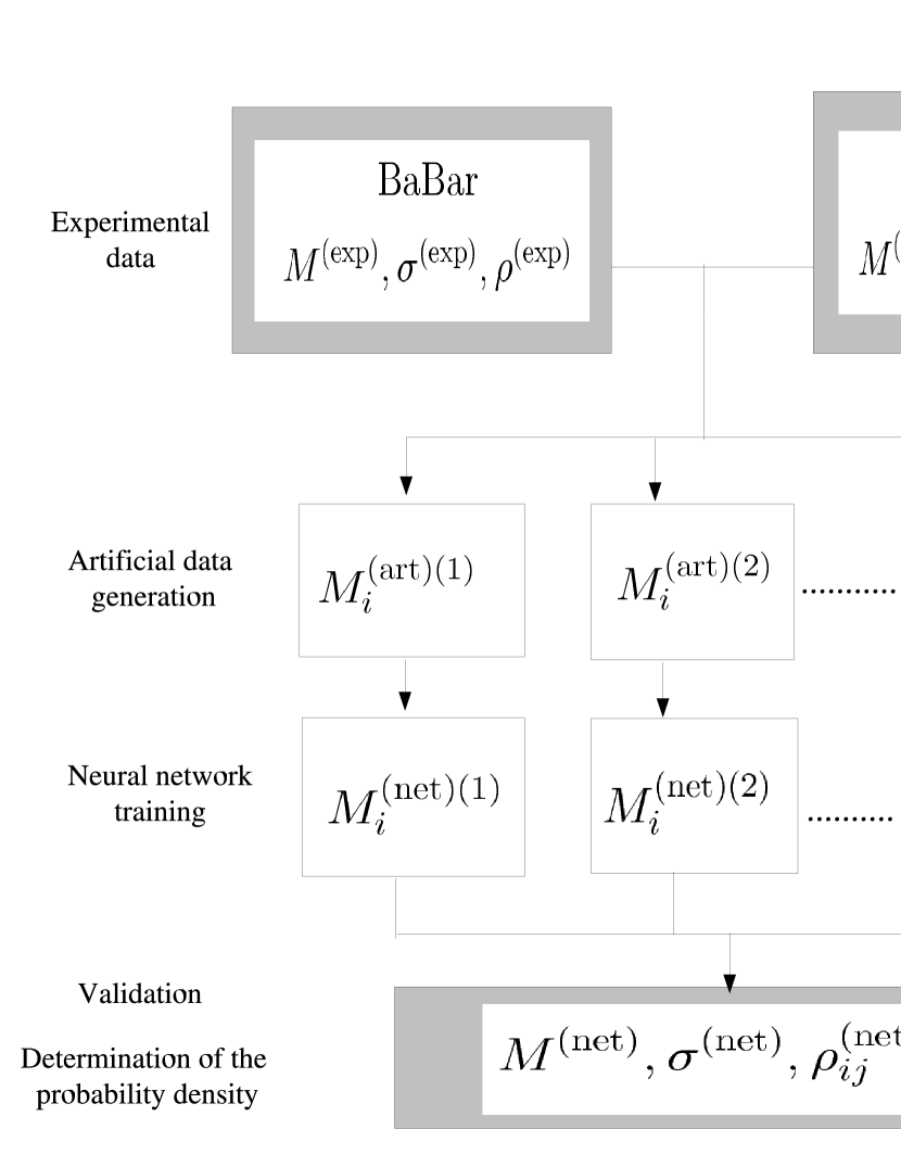
This success motivated us to implement this technique in the context of B physics. Therefore, in this work we construct an unbiased parametrization of the lepton energy spectrum is semileptonic B meson decays with a faithful estimation of the uncertainties. Since in Refs. [7, 8, 9, 11] the technique that will be used in this work is discussed in detail, here only those aspects which are special to the present application will be emphasized. Fig. 1 shows a diagram that summarizes our parametrization strategy.

Figure 1: Diagram that represents schematically our strategy to parametrize the lepton energy spectrum with a Monte Carlo sample of neural networks.

As a byproduct of our analysis an extraction of the heavy quark nonperturbative parameters $\bar{\Lambda}_{1S}$ and $\lambda_{1}$ will be performed using a technique that ensures that the associated theoretical uncertainties are minimized [14]. It will be shown that in this case the dominant uncertainties in the determination of these parameters turn out to be the experimental uncertainties, that is, those associated to the uncertainties in the parametrization of the spectrum.

Summarizing, there are three main motivations to construct a neural network parametrization of the lepton energy spectrum in B meson decays. The first one is to generalize the approach of Refs. [7, 8, 9, 10] to the problem of the construction of a unbiased determination of physical quantities with faithful estimation of their uncertainties from experimental data in the case for which the only available information on this quantity comes through truncated moments, as is the case for the lepton energy spectrum. Second, to show how this parametrization allows a more general comparison of theoretical predictions with data, since from our parametrization one can extract for example moments that have not been measured, like non-integer moments, higher order moments or moments with large cut in the lepton energy $E_{0}$, and use them for several purposes. In this work we examine two of such applications: the comparison of the theoretical accuracy with which higher order moments or moments with large $E_{0}$ are computed with respect to that of experimental measurements (Section 6.2), or novel methods to determine non perturbative parameters like $\overline{m}_{b}\left(\overline{m}_{b}\right)$ from non-integer moments (Section 7). Finally, the set of techniques described in the present work allow for a straightforward generalization to other relevant problems in B meson physics, like the determination of the B meson shape function from experimental data $S(\omega)$ [12].

The outline of this paper is as follows: in Section 2 we summarize the theoretical aspects of semileptonic B meson decays, and in Section 3 the experimental data that will be used. In Section 4 we describe the generation of Monte Carlo replicas of the experimental data, and in Section 5 the process of neural network training. In Section 6 we present the results that are obtained for the lepton energy spectrum and in Section 7 the determination of the nonperturbative parameters $\bar{\Lambda}_{1S}$ and $\lambda_{1}$. Finally, in Section 8 we conclude and briefly sketch possible new applications of our strategy to other problems in the context of B meson physics. Two appendices summarize the most technical details of the neural network parametrization.

2 Theory overview

Figure 2: Semileptonic decay of a B meson into a charmed final state

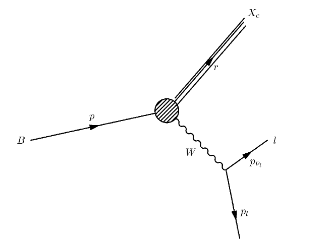
In this work the inclusive semileptonic decays of $B$ mesons with charmed final states will be considered. Therefore, the process that will be analyzed is $B\to X_{c}l\nu$, which is represented in Fig. 2. The differential decay rate for this process,

$$B(p)\to l(p_{l})+\bar{\nu}(p_{\bar{\nu}})+X_{c}(r)\ ,$$ (1)

depends on three different kinematical variables $q^{2},r$ and $E_{l}$, where $q=p_{l}+p_{\nu}$ is the total four momentum of the leptonic system, $r=p-q$ is the four-momentum of the charmed hadronic final state, with invariant mass $r^{2}=M_{X}^{2}$, and $E_{l}$ is the lepton energy in the rest frame of the B meson. This triple differential distribution can be decomposed, taking into account the kinematics of the process and the symmetries of the theory, in terms of three structure functions $W_{i}$,

$$\frac{d^{3}\Gamma}{dq^{2}drdE_{l}}(q^{2},r,E_{l})=\frac{G_{F}^{2}|V_{cb}|^{2}}{16\pi^{4}}\Bigg{[}\hat{q}^{2}W_{1}(\hat{q}^{2},\hat{u})-\qquad\qquad$$

$$\left(2v\cdot\hat{p}_{l}-2v\cdot\hat{p}_{l}v\cdot\hat{q}+\frac{\hat{q}^{2}}{2}\right)W_{2}(\hat{q}^{2},\hat{u})+\hat{q}^{2}\left(2v\cdot\hat{p}_{l}-v\cdot\hat{q}\right)W_{3}(\hat{q}^{2},\hat{u})\Bigg{]}\ ,$$ (2)

where $u^{2}=r^{2}-m_{c}^{2}$, $v=p/m_{b}$, and the quantities with a hat are dimensionless quantities normalized to $m_{b}$. All the structure functions $W_{i}(\hat{q}^{2},\hat{u})$ have both a perturbative expansion in powers of $\alpha_{s}$, and a nonperturbative expansion in powers of $1/m_{b}$, which can be computed in the framework of the heavy quark expansion. For example, the complete set of $\mathcal{O}(\alpha_{s})$ corrections for all the differential distributions that can be constructed from Eq. 2 with arbitrary kinematical cuts have recently become available [15, 16].

The most general observables that are accessible from the experiments, as it will be discussed below, are convolutions of differential distributions with suitable weight functions over a large enough range of energy, with kinematical cuts. A particular case of these observables are the moments of differential decay distributions. In this work the focus will be on leptonic moments, defined as

$$L_{n}(E_{0},\mu)\equiv\int_{E_{0}}^{E_{\max}}dE_{l}\left(E_{l}-\mu\right)^{n}\int dq^{2}dr\frac{d^{3}\Gamma}{dq^{2}drdE_{l}}(q^{2},r,E_{l})\ ,$$ (3)

where $E_{0}$ is a lower cut on the lepton energy, and $E_{\max}$ is the maximum energy allowed from the kinematics of the process that the lepton can have,

$$E_{\max}=\frac{m_{B}^{2}-m_{D}^{2}}{2m_{B}}\ ,$$ (4)

where $m_{B}$ is the average of the mass of the neutral and charged B mesons, and similarly for $m_{D}$. The lower cut in the lepton energy in Eq. 3 is imposed by experimental requirements, as will be discussed in the next section. The quantity that is going to be parametrized with a Monte Carlo sample of neural networks, the lepton energy distribution, is defined as

$$\frac{d\Gamma}{dE_{l}}(E_{l})\equiv\int dq^{2}dr\frac{d^{3}\Gamma}{dq^{2}drdE_{l}}(q^{2},r,E_{l})\ ,$$ (5)

that is related to the observable leptonic moments via

$$L_{n}(E_{0},\mu)=\int_{E_{0}}^{E_{\max}}dE_{l}\left(E_{l}-\mu\right)^{n}\frac{d\Gamma}{dE_{l}}(E_{l})\ .$$ (6)

The lepton energy spectrum, Eq. 5, in $B\to X_{c}l\nu$ decays, as has been discussed before, can be expanded in a power series both in $\alpha_{s}$ and in $1/m_{b}$. The leading order spectrum in both expansions is given by [6]

$$\frac{d\Gamma}{dy}\left(B\to X_{c}l\nu\right)=\Gamma_{0}2y^{2}\left[(1-f)^{2}(1+2f)(2-y)+(1-f)^{3}(1-y)\right]\theta(1-y-\rho)\ ,$$ (7)

$$f=\frac{\rho}{1-y},\qquad\rho=\frac{m_{c}^{2}}{m_{b}^{2}},\qquad y=\frac{2E_{l}}{m_{b}}\ ,$$ (8)

where

$$\Gamma_{0}=\frac{G_{F}^{2}m_{b}^{5}}{192\pi^{3}}$$ (9)

is the total parton model decay rate in the approximation of a massless final state quark. The kinematic support of the spectrum at this leading order partonic level is

$$E_{l}\in\left[0,\frac{m_{b}^{2}-m_{c}^{2}}{2m_{b}}\right]\ ,$$ (10)

where the upper limit is modified by nonperturbative (hadronic) corrections. The leading perturbative $\mathcal{O}(\alpha_{s})$ corrections to this spectrum have been known for some time [17], and there are estimations of the size of higher order terms though the BLM expansion [18]. The leading nonperturbative $\mathcal{O}(1/m_{b}^{2})$ corrections to the lepton energy spectrum where computed in Refs. [6, 19] and the $\mathcal{O}(1/m_{b}^{3})$ corrections in Ref. [20].

The total decay rate, obtained by integration of Eq. 5, admits the following heavy quark expansion [6, 21]:

$$\Gamma\left(B\to X_{c}l\nu\right)=\Gamma_{0}|V_{cb}|^{2}\left(1+A_{\mathrm{ew}}\right)A_{\mathrm{pert}}\cdot\quad$$

$$\Bigg{[}z_{0}(\rho)\left(1+\frac{\lambda_{1}}{2m_{b}^{2}}\right)+g(\rho)\frac{\lambda_{2}}{2m_{b}^{2}}+\mathcal{O}\left(\frac{1}{m_{b}^{3}}\right)\Bigg{]}\ ,$$ (11)

which depends up to $\mathcal{O}\left(1/m_{b}^{2}\right)$ on the the nonperturbative parameters $\lambda_{1}$ and $\lambda_{2}$, and where the phase space factors are given by

$$z_{0}(\rho)\equiv 1-8\rho+8\rho^{3}-\rho^{4}-12\rho^{2}\log\rho,\quad\rho=\frac{m_{c}^{2}}{m_{b}^{2}}\ ,$$ (12)

$$g(\rho)=-9+24\rho-72\rho^{2}+72\rho^{3}-15\rho^{4}-36\rho^{2}\ln\rho\ ,$$ (13)

and where $A_{\mathrm{ew}}$ stands for the electroweak corrections and $A_{\mathrm{pert}}$ for the QCD perturbative corrections. Similar heavy quark expansions are available for the lepton energy moments (see Ref. [2] and references therein).

3 Experimental data

The experimental data that will be used in the present analysis consists on moments with kinematical cuts of the lepton energy distribution in semileptonic B meson decays to charmed final states $B\to X_{c}l\nu$. These moments have recently been measured with great accuracy at the B factories, Babar [22] and Belle [24], as well as by Cleo [25]. Therefore, in the present analysis the latest data from these three experiments will be used. Data from CDF [26] is not incorporated since it is restricted to hadronic moments.

As it has been mentioned before, the main experimental difficulty for the measurement of the lepton energy spectrum for low values of the lepton energy is the fact that for low lepton energies the background from other decay modes dominates, and it is challenging to disentangle the desired decay mode. Therefore, kinematical cuts have to be imposed that remove the low $E_{l}$ region of the spectrum. Another relevant consideration is that the reference frame change, from the laboratory frame to the B meson rest frame and several experimental corrections, like for example electroweak final state radiation, are easier to perform in terms of moments of the distribution. Therefore the final published measurements are moments of the lepton energy spectrum, Eq. 6, with different cuts in the lepton energy, rather than the full spectrum itself.

Now the data that will be used for the present parametrization of the lepton energy spectrum will be described. The Babar Collaboration [22] provides the partial branching ratios,

$$M_{0}(E_{0})=\tau_{B}L_{0}(E_{0},0)=\tau_{B}\int_{E_{0}}^{E_{\max}}\frac{d\Gamma}{dE_{l}}(E_{l})~{}dE_{l}\ ,$$ (14)

where $\tau_{B}$ is the average B meson lifetime [23], the first moment,

$$M_{1}(E_{0})=\frac{L_{1}(E_{0},0)}{L_{0}(E_{0},0)}\ ,$$ (15)

and the central moments,

$$M_{n}(E_{0})=\frac{L_{n}(E_{0},M_{1}(E_{0}))}{L_{0}(E_{0},0)},\qquad n=2,3\ ,$$ (16)

for five different values of $E_{0}$ from 0.6 to 1.5 GeV, which makes a total of 20 data points. The rationale for extracting Eq. 16 rather than for example

$$\widetilde{M}_{n}(E_{0})=\frac{L_{n}(E_{0},0)}{L_{0}(E_{0},0)},\qquad n=2,3\ ,$$ (17)

is that in the former case correlations between different moments are smaller and therefore more independent information can be extracted from the measurements.

The Belle Collaboration [24] provides the same moments, $M_{n}(E_{0})$ for $n=1$, $n=2$ and $n=3$. The difference with the Babar data is that the partial branching ratio Eq. 14 is not measured, and that the Belle data cover a somewhat larger lepton energy range, since the lowest value of $E_{0}$ of their data set is $E_{0}=0.4$ GeV. These moments, for six different values of $E_{0}$ from 0.4 to 1.5 GeV, make up a total of 18 data points. Finally the Cleo Collaboration [25] provides the moments $M_{n}(E_{0})$ for $n=1,2$, for energies between 0.6 to 1.5 GeV, for a total of 20 data points (10 data points for $n=1$ and 10 data points for $n=2$). The average correlations for this experiment are larger since measurements of the same moment at different energies $E_{0}$ are highly correlated.

The three collaborations provide also the total and statistical errors, as well as the correlation between different measurements. These features are summarized in Table 1. Note that for all experiments correlations are rather large, so it is compulsory to incorporate them in a consistent way in the statistical analysis of the data. However, one has to be careful with the treatment of the experimental correlations, for reasons to be described on the next section.

Note that the results of this work, summarized in section 6, consist on a parametrization of experimental data without the need for any theoretical input. The uncertainties associated to the parametrization of the lepton spectrum will therefore be reduced if experimental measurements of lepton spectrum moments are measured with larger accuracy in the future.

3.1 Treatment of experimental correlations

As has been already noticed, for example see the global analysis of B decays of Ref. [41], it can be checked that the experimental correlation matrices, $\rho_{ij}^{(\mathrm{exp})}$, as presented with the published data of the three experiments [24, 22, 25], are not positive definite. The source of this problem can be traced to the fact that off-diagonal elements of correlation matrix are large, as expected since moments with similar energy cuts contain almost the same amount of information and are therefore highly correlated. Then one can check that some eigenvalues are negative and small, and this points to the fact that the source of the problem is an insufficient accuracy in the computation of the elements of the correlation matrix.

However, whatever is the original source of the problem, the fact that the experimental correlation matrices are not positive definite has an important consequence: the technique introduced in [7] for the generation of a sample of replicas of the experimental data in a way that correlations are incorporated relies on the existence of a positive definite correlation matrix, and therefore if this is not the case our technique cannot be applied.

A method to overcome these difficulties while keeping the maximum amount on information on experimental correlations as possible consists on removing those data points for which the experimental correlations are larger than a maximum correlation, $\rho_{ij}^{(\exp)}\geq\rho^{\max}$. The value of $\rho^{\max}$ is determined separately for each experiment as the maximum value for which the resulting correlation matrix is positive definite. In Table 2 the values of $\rho^{\max}$ for each experiment are shown, together with the features of the remaining experimental data after those data points with too large correlations have been removed. In the case of the Belle measurements, another problem with the correlation matrix is that the contribution to the correlation coefficients from systematic uncertainties has at present not been incorporated.

Experiment	$N_{\mathrm{dat}}$	$n$	$E_{0}$ (GeV)	$\left\langle\sigma_{\mathrm{stat}}\right\rangle$	$\left\langle\sigma_{\mathrm{tot}}\right\rangle$	$\left\langle|\rho|\right\rangle$
Babar [22]	20	0 - 3	0.6 - 1.5	6.0%	8.0%	0.50
Belle [24]	18	1 - 3	0.4 - 1.5	15.0%	16.0%	0.34
Cleo[25]	20	1 - 2	0.6 - 1.5	1.0%	1.3%	0.65

Table 1: Features of experimental data on lepton moments $M_{n}(E_{0})$. Note that averages over experimental errors are given as percentages.

Experiment	$N_{\mathrm{dat}}$	$n$	$E_{0}$ (GeV)	$\left\langle\sigma_{\mathrm{stat}}\right\rangle$	$\left\langle\sigma_{\mathrm{tot}}\right\rangle$	$\rho^{\max}$	$\left\langle|\rho|\right\rangle$
Babar [22]	16	0 - 3	0.6 - 1.5	4.0%	5.0%	0.97	0.49
Belle [24]	15	1 - 3	0.4 - 1.5	18.0%	19.0%	0.88	0.31
Cleo [25]	10	1 - 2	0.6 - 1.5	0.5%	1.0%	0.95	0.69

Table 2: Features of experimental data that is included in the fit, after data points with too large correlations have been removed. Note that averages over experimental error are given as percentages.

4 Replica generation

As has been mentioned in the Introduction, in this work the strategy of Ref. [7] is followed to parametrize the lepton energy spectrum from the experimental information on its moments. The first step of this technique is to generate an ensemble of Monte Carlo replicas of the original experimental data, which consists in the measured moments, which will be denoted by

$$M_{i}^{(\mathrm{exp})},\quad i=1,\ldots,N_{\mathrm{dat}}\ ,$$ (19)

where $M_{i}^{(\mathrm{exp})}$ stands for any of Eqns. 14-16, and $N_{\mathrm{dat}}$ is the total number of experimental data points, together with the total error and the correlation matrix.

To generate replicas one proceeds as follows: the k$-$th artificial replica of the experimental data $M^{(\mathrm{art})(k)}$ is constructed as

$$M_{j}^{(\mathrm{art})(k)}=M_{j}^{(\mathrm{exp})}+s^{(k)}_{j}\sigma^{(\mathrm{exp})}_{j,\mathrm{tot}}\ ,\quad j=1,\ldots,N_{\mathrm{dat}},\quad,k=1,\ldots,N_{\mathrm{rep}}\ ,$$ (20)

where $s^{(k)}_{j}$ are gaussian random numbers with same correlation matrix as the experimental correlation matrix $\rho_{ij}$, $\sigma^{(\mathrm{exp})}_{j,\mathrm{tot}}$ is the total error of the j-th data point and $N_{\mathrm{rep}}$ is the number of generated replicas of the experimental data. This way the ensemble of replicas is not only able to reproduce the central values and the errors but also the correlations of the experimental data.

As explained in Ref. [7], the size of the replica sample is fixed by the condition that the averages over replicas reproduce the experimental values for central values, errors and correlations. The different statistical estimators are defined in Appendix B. In Table 3 the relevant statistical estimators for the replica generation are summarized. One can observe that to reach the desired accuracy of a few percent and to have scatter correlations $r\geq 0.99$ for central values, errors and correlations, a sample of 1000 replicas is needed.

$N_{\mathrm{rep}}$	10	100	1000
$\left\langle PE\left[\left\langle M\right\rangle_{\mathrm{rep}}\right]\right\rangle$	2.47%	0.40%	0.24%
$\left\langle PE\left[\sigma^{(\mathrm{art})}\right]\right\rangle_{\mathrm{dat}}$	32.4%	13.8%	3.4%
$\left\langle\sigma^{(\mathrm{art})}\right\rangle_{\mathrm{dat}}$	0.00265	0.00277	0.00268
$r\left[\sigma^{(\mathrm{art})}\right]$	0.95	0.99	0.99
$\left\langle PE\left[\rho^{(\mathrm{art})}\right]\right\rangle_{\mathrm{dat}}$	60.1%	19.6%	6.7%
$\left\langle\rho^{(\mathrm{art})}\right\rangle_{\mathrm{dat}}$	0.132	0.138	0.155
$r\left[\rho^{(\mathrm{art})}\right]$	0.75	0.96	0.99
$\left\langle\mathrm{cov}^{(\mathrm{art})}\right\rangle_{\mathrm{dat}}$	$1.1~{}10^{-6}$	$1.4~{}10^{-6}$	$1.3~{}10^{-6}$
$r\left[\mathrm{cov}^{(\mathrm{art})}\right]$	0.86	0.98	0.99

Table 3: Comparison between experimental and Monte Carlo data. The experimental data have $\left\langle\sigma^{(\mathrm{exp})}\right\rangle_{\mathrm{dat}}=0.00267$ , $\left\langle\rho^{(\mathrm{exp})}\right\rangle_{\mathrm{dat}}=0.166$ and $\left\langle\mathrm{cov}^{(\mathrm{exp})}\right\rangle_{\mathrm{dat}}=1.4~{}10^{-6}$, for a total of 41 data points.

5 Neural network training strategy

As described in Ref. [7], the next step of our strategy is to train a neural network to each of the replicas of the experimental data. Artificial neural networks (see Fig. 3) are highly nonlinear mappings between input and output patterns, defined by its parameters, called weights $\omega_{ij}^{(l)}$ and thresholds $\theta_{i}^{(l)}$. They provide unbiased robust universal approximants to incomplete or noisy data, and they interpolate between data points with the only assumption of smoothness. A neural network is a suitable way of parametrizing experimental data since it is a most unbiased prior, and moreover in combination with the Monte Carlo methods it provides a faithful estimation of the uncertainties associated to this parametrization.

Figure 3: Schematic representation of an artificial neural network.

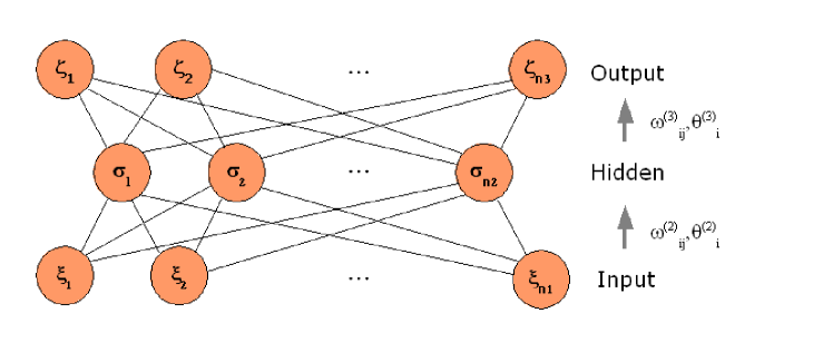
In this work a particular class of neural networks called feed-forward perceptrons are used. For this class of neural networks, the relation that gives the values (activation states) of the i-th neuron in the l-th layer $\xi^{(l)}_{i}$ depends on the activation states of the neurons in the previous layer,

$$\xi^{(l)}_{i}=g\left(h_{i}^{(l)}\right)\ ,\quad i=1,\ldots,n_{l},\quad l=1,\ldots,L\ ,$$ (21)

$$h_{i}^{(l)}=\sum_{j=1}^{n_{l-1}}\omega_{ij}^{(l)}\xi_{j}^{(l-1)}+\theta_{i}^{(l)}\ ,$$ (22)

where $\theta_{i}^{(l)}$ is the activation threshold of the neuron, $L$ the total number of layers of the network and $n_{l}$ the number of neurons in each layer. The function $g(x)$ is the activation function of the neuron, which is taken to be a sigmoid in the inner layers,

$$g(x)=\frac{1}{1+\exp(-x)}\ ,$$ (23)

and a linear activation function $g(x)=x$ for the last neuron to increase the sensitivity of the network. For illustrative purposes, let us consider a simple neural network, which consists on two input neurons and one output neuron. If $\xi_{1}^{(1)}$ and $\xi_{2}^{(2)}$ are the values of the input neurons, then the value of the output neuron $\xi^{(2)}_{1}$ will be, from Eqns. 21 and 22,

$$\xi^{(2)}_{1}=f\left(\xi_{1}^{(1)},\xi_{2}^{(2)}\right)=\left[1+\exp\left(-\omega_{11}^{(1)}\xi_{1}^{(1)}-\omega_{12}^{(1)}\xi_{2}^{(1)}\right)\right]^{-1}\ .$$ (24)

From the above explicit example it is clear that a neural network is a nonlinear function that relates the input values with the output values.

Therefore, the lepton energy spectrum is parametrized with a neural network,

$$\left(\frac{d\Gamma}{dE_{l}}\right)^{(\mathrm{net})}(E_{l})\,$$ (25)

where $E_{l}$ is the lepton energy, so that if $E_{l}$ is the input of the neural network, then $\left(d\Gamma/dE_{l}\right)^{(\mathrm{net})}$ is the associated output.

Training a neural network means the determination of its parameters (the neuron weights and thresholds) to minimize a suitable statistical estimator. In our case for each replica the diagonal error will be minimized, defined as

$${\chi^{2}}^{(k)}=\frac{1}{N_{\mathrm{dat}}}\sum_{i=1}^{N_{\mathrm{dat}}}\frac{\left(M_{i}^{(\mathrm{art})(k)}-M_{i}^{(\mathrm{net})(k)}\right)^{2}}{\sigma^{(\mathrm{exp})2}_{i,\mathrm{tot}}}\ ,\qquad k=1,\ldots,N_{\mathrm{rep}}\ ,$$ (26)

where $M_{i}^{(\mathrm{net})(k)}$ is the i-th moment as computed from the k-th neural network, which is trained on the k-th replica of the experimental data, and $\sigma^{(\mathrm{exp})}_{i,\mathrm{tot}}$ is the total error of the i-th data point.

The minimization technique that will be used for the neural network training is genetic algorithms, a minimization strategy that has been used in different high energy physics applications[29] . This method is specially suitable to find the global minima of highly nonlinear problems, as the one that is being discussed in this work. Other standard deterministic minimization strategies, like for example MINUIT, are not suitable for this problem since the parameter space is very large. Genetic algorithms minimization is divided in steps called generations, so the number of generations of a given neural network training corresponds to the training length of the genetic algorithms minimization process.

Figure 4: Comparison of fits it to the experimental data with different neural network architectures

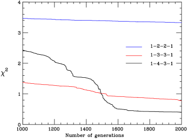
As has been discussed previously in detail [7], the choice of the architecture of the neural network (the number of layers and the number of neurons in each layer) cannot be derived from general rules and it must be tailored to each specific problem. In particular the neural network has to be redundant, that is, it has to have a larger number of parameters than the minimum number required to satisfactorily fit the patterns that have to be learnt, in this case experimental data. However, the architecture cannot be arbitrarily large because then the training length gets very large. In this case one finds that an acceptable compromise is given by an architecture 1-4-3-1. A suitable criterion to choose the optimal architecture is to take the architecture which is next to the first stable architecture, that is, the first architecture that can fit the data and gives the same fit that an architecture with one less neuron. This way one is sure that the neural network is redundant for the problem that is considered. Fig. 4 shows a training to the experimental data with three different architectures: first one observes that 1-2-2-1 is not capable to fit properly the data, but a more complex architecture 1-3-3-1 can fit this data. Therefore, the architecture 1-4-3-1 is taken as the reference architecture for the parametrization of the lepton energy spectrum.

The training of a neural network does not follow general rules either, and the optimal minimization strategy must be determined for each particular problem. In the present situation the training strategy that is adopted is the following: there is a single training epoch in which the $\chi^{2(k)}$, Eq. 26, is minimized with dynamical stopping of the training of the replicas. That is, for each replica, the training is stopped either when the condition $\chi^{2(k)}\leq\chi^{2}_{\mathrm{stop}}$ is satisfied or when the maximum number of generations $N_{gen}$ is reached. One finds that $\chi^{2}_{\mathrm{stop}}=2$ and $N_{\mathrm{gen}}=3000$ are suitable choices. On top of that, the neural network weights are initialized between $\left[-\omega_{\mathrm{init}}/2,\omega_{\mathrm{init}}/2\right]$ randomly, with $\omega_{\mathrm{init}}=10$. The rationale for this choice is that it can be observed that the natural value for the neural network weights is $\mathcal{O}\left(10^{1}\right)$, so the fit will be faster if the initial values for the neural network weights are of the same order of magnitude.

Finally, in the training of the replicas the so-called weighted training will be used for the genetic algorithms minimization. As it has been shown in Refs. [7, 8], it is in general useful to weight during the training the different experiments according to their $\chi^{2}$, so that more weight is given to those experiments with a larger value of their $\chi^{2}$, so that the final $\chi^{2}$ is more homogeneous than in the unweighted case. The essential idea of this technique is that the minimized $\chi^{2}_{\mathrm{minim}}$ is given by

$$\chi^{2}_{\mathrm{minim}}=\frac{1}{N_{\mathrm{dat}}}\sum_{j=1}^{N_{\mathrm{exp}}}w_{j}N_{\mathrm{dat},j}\chi^{2}_{j}\ ,$$ (27)

where $N_{\mathrm{dat},j}$ is the number of data points and $\chi^{2}_{j}$ the value of the $\chi^{2}$, Eq. 26, of the j-th experiment. One finds after a detailed analysis that the values $w_{\mathrm{Babar}}=0.3$, $w_{\mathrm{Belle}}=2$ and $w_{\mathrm{Cleo}}=0.5$ are suited to obtain a more even $\chi^{2}_{j}$ distribution between experiments.

5.1 Compatibility between experiments

Figure 5: $\chi^{2}$, Eq. 26, of the different experiments, for a fit to the experimental data including all experiments.

Figure 6: $\chi^{2}$ of the different experiments when only the Babar data is fitted.

Figure 7: Same as in Fig. 7, but now only the Belle data is fitted.

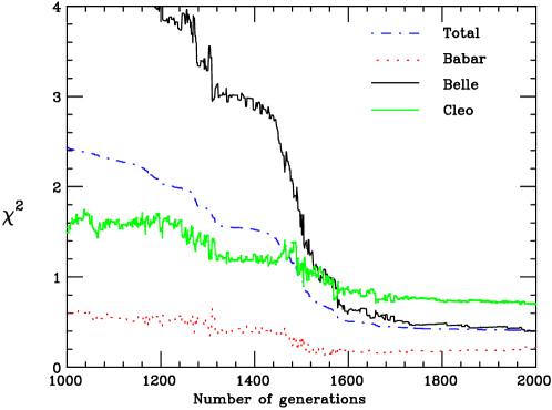
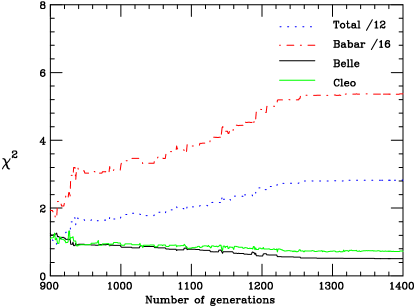
In global analysis of experimental data which consist of different experiments, as it is the case now (with Babar, Belle and Cleo), one has also to address the issue of possible inconsistencies between different experiments, that is, the possibility that a subset of points from two experiments in the same region of the parameter space do not agree with each other within experimental errors. This issue is of paramount importance in the context of global parton distribution fits, see for example [31, 8]. In the present application, it can be seen that the three experiments yield compatible results, as was already known from global fits to B decay data.

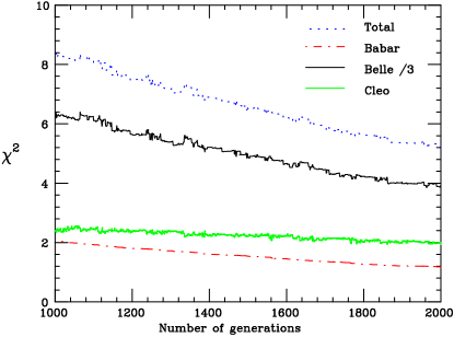
This compatibility can be shown in a different number of ways. For example, training only one experiment and checking whether or not the other experiments can be predicted, that is, whether they have a low $\chi^{2}$ even if they are not incorporated in the fit. In Fig. 5 we show a fit to the experimental data for which all three experiments (Babar, Belle and Cleo) are incorporated in the fit. One observes that at the end of the training all experiments satisfy $\chi^{2}\ll 1$. In Fig. 7 show the results of a fit when only Babar is incorporated in the fit, and in Fig. 7 the same fit with this time with data from the Belle experiment only. Note that when only a single experiment is incorporated in the fit, like in Figs. 7 and 7, only the $\chi^{2}$ of that experiment is expected to decrease, while the total $\chi^{2}$ might decrease slower or even grow.

It is observed that the three experiments are not only compatible but also complementary. In particular Cleo is predicted by both Belle and Babar (as expected since the kinematical coverage of the Cleo experiment is included in the other two experiments), while Belle and Babar cannot predict each other, as a consequence of the fact that different regions in the parameter space are covered by the two experiments: only Babar has experimental data on the $n=0$ moment (partial decay rate), while only Belle has data at the lowest lepton energy ($E_{0}=0.4$ GeV). It will be shown in Section 6 that also for the correct estimation of the uncertainties the inclusion of data from different experiments is crucial.

5.2 Kinematical constraints

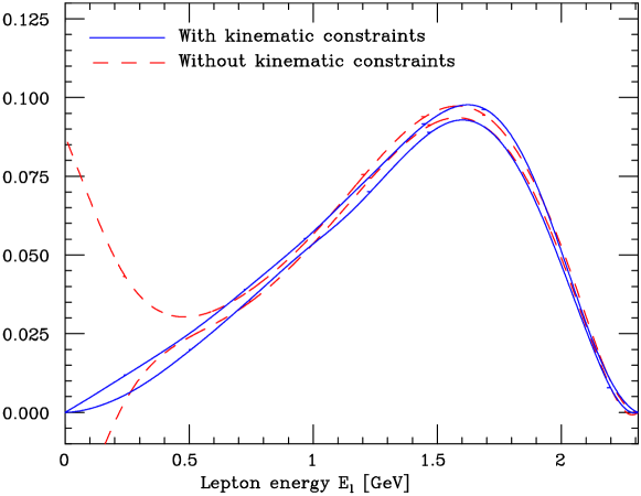
The lepton spectrum, Eq. 5, has to satisfy three constraints independently of the dynamics of the process. First of all, it vanishes outside the region where it has kinematical support, in particular it has to vanish at the kinematical endpoints, $E_{l}=0$ and $E_{l}=E_{\max}$. Second, the spectrum is a positive definite quantity (since any integral over it is an observable, a partial branching ratio), therefore, it must satisfy a local positivity condition.

There are several methods to introduce kinematical constraints in our parametrization. It has been found that for the present application, the optimal method to implement the kinematical constraint that the spectrum should vanish at the endpoints is to hard-wire them into the parametrization, that is, the lepton energy spectrum parametrized by a neural network will be given by

$$\left(\frac{d\Gamma}{dE_{l}}\right)^{(\mathrm{net})}(E_{l})=E_{l}^{n_{1}}\xi_{1}^{(L)}(E_{l})(E_{\max}-E_{l})^{n_{2}}$$ (28)

with $n_{1},n_{2}$ positive numbers, and $\xi_{1}^{(L)}$ is the output of the neural network for a given value of $E_{l}$. The assumption of this functional behavior at the endpoints of the spectrum introduces no bias since, as will be shown in Section 6, our results do not depend on the value of $n_{1},n_{2}$. For the reference training the values $n_{1}=1$ and $n_{2}=1$ have been chosen.

The remaining kinematical constraint, the positivity constraint, is imposed as a Lagrange multiplier in the total error. That is, the quantity to be minimized, $\chi^{2}_{\mathrm{tot},\mathrm{min}}$, is the sum of two terms,

$$\chi^{2}_{\mathrm{tot},\mathrm{min}}=\chi^{2}_{\mathrm{dat}}+\chi^{2}_{\mathrm{pos}}\ ,$$ (29)

where the contribution from experimental data $\chi^{2}_{\mathrm{dat}}$ is Eq. 26 and the contribution from the positivity constraint is defined as

$$\chi^{2}_{\mathrm{pos}}=\lambda P\left[\left(\frac{d\Gamma}{dE_{l}}\right)^{(\mathrm{net})}\right]\ ,$$ (30)

where the positivity condition is implemented in a way that those configurations in which a region of the spectrum is negative are penalized,

$$P\left[\left(\frac{d\Gamma}{dE_{l}}\right)^{(\mathrm{net})}\right]=-\int_{0}^{E_{\max}}dE_{l}\left(\frac{d\Gamma}{dE_{l}}\right)^{(\mathrm{net})}(E_{l})\theta\left(-\left(\frac{d\Gamma}{dE_{l}}\right)^{(\mathrm{net})}(E_{l})\right),$$ (31)

since P is zero for a positive spectrum, and leads to a positive contribution to the total error function, Eq. 29 if some part of the lepton spectrum is negative. The relative weight $\lambda$ in Eq. 30 is determined via a stability analysis, with the requirement that $\lambda$ is large enough so that the constraint is verified, but small enough so that experimental data can still be learned in an efficient way. It has been found that $\lambda=10^{10}$ satisfies the above requirements. As will be proved in the next section, the implementation of the kinematical constraints plays a essential role in the parametrization of the lepton spectrum.

6 Results

Figure 8: The 1-$\sigma$ uncertainty band for the lepton energy spectrum, Eq. 5, as parametrized by the Monte Carlo ensemble of neural networks.

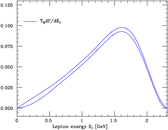
In this section the results on the parametrization of the lepton energy spectrum are presented. These results consist on the sample of trained neural networks, from which averages and moments can be computed with the associated uncertainties. The most technical details of these results for neural network parametrization and the associated statistical validation can be found in Appendix A.

6.1 Lepton energy spectrum

In figure 8 the lepton energy spectrum with uncertainties is represented. For illustration, let us recall how the central value and the spread of this spectrum are computed from the neural network sample. For the average one has

$$\left\langle\left(\frac{d\Gamma}{dE_{l}}\right)^{(\mathrm{net})}\right\rangle(E_{l})=\frac{1}{N_{rep}}\sum_{k=1}^{N_{\mathrm{rep}}}\left(\frac{d\Gamma}{dE_{l}}\right)^{(\mathrm{net})(k)}(E_{l})\ ,$$ (32)

while for the spread the appropriate expression is

$$\sigma^{(\mathrm{net})2}_{d\Gamma/dE_{l}}(E_{l})=\left\langle\left(\frac{d\Gamma}{dE_{l}}\right)^{(\mathrm{net})2}\right\rangle(E_{l})-\left[\left\langle\left(\frac{d\Gamma}{dE_{l}}\right)^{(\mathrm{net})}\right\rangle\right]^{2}(E_{l})\ .$$ (33)

In Fig. 8 the $1-\sigma$ envelope of the lepton spectrum is plotted, where the central value has been computed with Eq. 32 and the standard deviation with Eq 33. Note that the error is rather small for large values of the lepton energy $E_{l}\geq 1.8$ GeV, and it grows for smaller values of $E_{l}$. The error bands for the other plots are computed in the same way.

As discussed before, the sample of trained neural network reproduce the correlations of the experimental data. For instance, imagine that one is interested in the correlation between two moments of the lepton spectrum, $M_{n_{1}}(E_{01})$ and $M_{n_{2}}(E_{02})$, of arbitrary order and arbitrary lepton energy cut. With the probability measure of the lepton energy spectrum constructed in this work, this correlation $\rho_{12}\equiv\rho\left(n_{1},E_{01},n_{2},E_{02}\right)$ is given by

$$\rho_{12}=\frac{\left\langle M_{n_{1}}^{(\mathrm{net})}(E_{01})M_{n_{2}}^{(\mathrm{net})}(E_{02})\right\rangle_{\mathrm{rep}}-\left\langle M_{n_{1}}^{(\mathrm{net})}(E_{01})\right\rangle_{\mathrm{rep}}\left\langle M_{n_{2}}^{(\mathrm{net})}(E_{02})\right\rangle_{\mathrm{rep}}}{\sqrt{\left\langle M_{n_{1}}^{(\mathrm{net})}(E_{01})^{2}\right\rangle_{\mathrm{rep}}-\left\langle M_{n_{1}}^{(\mathrm{net})}(E_{01})\right\rangle_{\mathrm{rep}}^{2}}\sqrt{\left\langle M_{n_{2}}^{(\mathrm{net})}(E_{02})^{2}\right\rangle_{\mathrm{rep}}-\left\langle M_{n_{2}}^{(\mathrm{net})}(E_{02})\right\rangle_{\mathrm{rep}}^{2}}}\ ,$$ (34)

where averages over the sample of neural networks are computed in the standard way, for instance

$$\left\langle M_{n_{1}}^{(\mathrm{net})}(E_{01})M_{n_{2}}^{(\mathrm{net})}(E_{02})\right\rangle_{\mathrm{rep}}=\frac{1}{N_{\mathrm{rep}}}\sum_{k=1}^{N_{\mathrm{rep}}}M_{n_{1}}^{(\mathrm{net})(k)}(E_{01})M_{n_{2}}^{(\mathrm{net})(k)}(E_{02})\ ,$$ (35)

and similarly for the remaining averages. This examples clarifies that fact that not only central values and total errors from experimental data, showed in Fig. 8, but also correlations are present in the parametrization of the lepton energy spectrum.

As it has been explained in [7], it is crucial to validate the results of the parametrization with suitable statistical estimators. In Table 4 the most relevant statistical estimators for all the data points are summarized, and in Table 5 one has the same estimators for the different experiments included in the fit. A more detailed analysis of these estimators is found in Appendix A.

It has been checked that the large value of $\chi^{2}$ of the BELLE experiment is not because globally their data is not properly fitted (as can be seen in the plots), but that it is only due to two points, $n=2,3$, $E_{0}=1.5$ GeV that have an anomalously large $\chi^{2}$. If those two points are not included then $\chi^{2}_{\mathrm{tot},\mathrm{Belle}}=0.92$. These two points are systematically below Babar data with errors half as small. This is similar as what happened with the NMC experiment is the proton structure function fits described in Ref. [7].

	10	100	1000
$\chi^{2}_{\mathrm{tot}}$	1.31	1.18	1.21
$\left\langle\chi^{2}\right\rangle$	2.50	2.28	2.33
$\left\langle PE\left[\left\langle M\right\rangle_{\mathrm{rep}}\right]\right\rangle$	9%	8%	8%
$r\left[M\right]$	0.999	0.999	0.999
$\left\langle PE\left[\sigma^{(\mathrm{net})}\right]\right\rangle_{\mathrm{dat}}$	67%	58%	45%
$\left\langle\sigma^{(\exp)}\right\rangle_{\mathrm{dat}}$	0.00267	0.00267	0.00267
$\left\langle\sigma^{(\mathrm{net})}\right\rangle_{\mathrm{dat}}$	0.00180	0.00169	0.00187
$r\left[\sigma^{(\mathrm{net})}\right]$	0.77	0.85	0.86
$\left\langle\rho^{(\exp)}\right\rangle_{\mathrm{dat}}$	0.166	0.166	0.166
$\left\langle\rho^{(\mathrm{net})}\right\rangle_{\mathrm{dat}}$	0.320	0.245	0.324
$r\left[\rho^{(\mathrm{net})}\right]$	0.35	0.38	0.38
$\left\langle\mathrm{cov}^{(\exp)}\right\rangle_{\mathrm{dat}}$	$1.4~{}10^{-6}$	$1.4~{}10^{-6}$	$1.4~{}10^{-6}$
$\left\langle\mathrm{cov}^{(\mathrm{net})}\right\rangle_{\mathrm{dat}}$	$7.8~{}10^{-7}$	$6.7~{}10^{-7}$	$1.0~{}10^{-6}$
$r\left[\mathrm{cov}^{(\mathrm{net})}\right]$	0.49	0.53	0.53

Table 4: Statistical estimators for the ensemble of trained neural networks, for 10, 100 and 1000 trained replicas

	Babar	Belle	Cleo
$\chi^{2}_{\mathrm{tot}}$	0.42	2.06	1.22
$\left\langle\chi^{2}\right\rangle$	1.67	3.13	2.21
$\left\langle PE\left[\left\langle M\right\rangle_{\mathrm{rep}}\right]\right\rangle$	2.3%	18.1%	0.6%
$r\left[M\right]$	0.999	0.999	0.999
$\left\langle PE\left[\sigma^{(\mathrm{net})}\right]\right\rangle_{\mathrm{dat}}$	34%	44%	65%
$\left\langle\sigma^{(\exp)}\right\rangle_{\mathrm{dat}}$	0.0023	0.0021	0.0041
$\left\langle\sigma^{(\mathrm{net})}\right\rangle_{\mathrm{dat}}$	0.0018	0.0017	0.0022
$r\left[\sigma^{(\mathrm{net})}\right]$	0.94	0.89	0.83
$\left\langle\rho^{(\exp)}\right\rangle_{\mathrm{dat}}$	0.16	0.40	0.31
$\left\langle\rho^{(\mathrm{net})}\right\rangle_{\mathrm{dat}}$	0.15	0.28	0.51
$r\left[\rho^{(\mathrm{net})}\right]$	0.87	0.29	0.31
$\left\langle\mathrm{cov}^{(\exp)}\right\rangle_{\mathrm{dat}}$	$6.9~{}10^{-6}$	$1.5~{}10^{-6}$	$6.5~{}10^{-7}$
$\left\langle\mathrm{cov}^{(\mathrm{net})}\right\rangle_{\mathrm{dat}}$	$2.0~{}10^{-5}$	$1.2~{}10^{-6}$	$1.8~{}10^{-6}$
$r\left[\mathrm{cov}^{(\mathrm{net})}\right]$	0.98	0.58	-0.21

Table 5: Statistical estimators for the ensemble of trained neural networks, for those experiments included in the fit. The replica sample consists of 1000 neural networks.

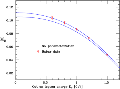
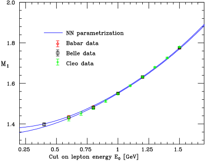
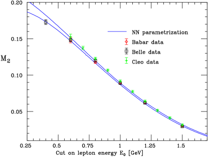
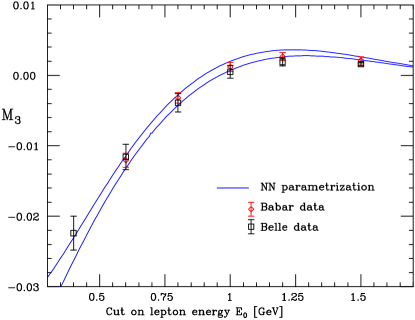
In Figs. 10 to 12 the computation of the moments of the lepton energy spectrum from our parametrization is compared to the experimental data from Babar, Belle and Cleo, and good agreement for all the data points is observed. Note that some of the experimental data points have not been included in the training, for the reasons discussed in Section 3.1, but nevertheless the lepton energy parametrization is in good agreement also with those data points.

To asses the relevance of the implementation of kinematical constraints into our neural network parametrization of the lepton spectrum, it is instructive to compare fits with and without the inclusion of kinematical constraints. In Fig. 13 one can observe that when the endpoint constraint at $E_{l}=0$ and the positivity constraint are removed the error becomes very large at small $E_{l}$. This is so because experimental data does not constrain the value of the lepton spectrum for low values of $E_{l}$. Note that the physical value for the spectrum at the endpoint, $\left(d\Gamma/dE_{l}\right)(E_{l}=0)=0$, is contained within the small-$E_{l}$ error bars.

Figure 9: Comparison of the partial branching ratio, Eq. 14 obtained from our parametrization with the experimental measurements, as a function of the lower cut on the lepton energy $E_{0}$.

Figure 10: Same as. Fig 10 for the first moment $M_{1}$, Eq. 15

Figure 11: Same as Fig. 10 for the second moment, $M_{2}$, Eq. 16.

Figure 12: Same as Fig. 10 for the third moment, $M_{3}$, Eq. 16.

Figure 13: Lepton energy spectrum when no kinematic constraints are incorporated in the fit. One one can see in this case the error at small $E_{l}$ grows very large and the extrapolation to $E_{0}=0$ becomes unreliable.

Figure 14: Lepton energy spectrum when only Babar data is incorporated in the fit.

Figure 15: Comparison of the lepton energy spectrum when the for different values of the parameters $n_{1}$ and $n_{2}$

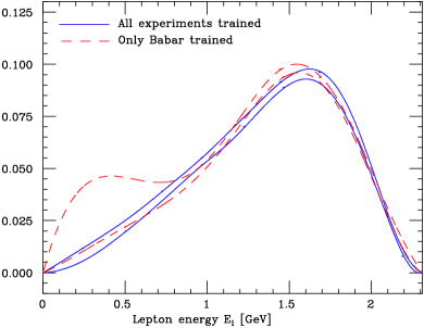
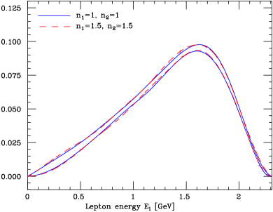
To estimate the contribution of the different experiments to the global fit, it is interesting to compare (see Fig. 15) a fit in which only one experiment, Babar is incorporated in the fit. It can be observed that when only the Babar data is fitted, the error at small values of $E_{l}$ is much larger. This is so because, as discussed above, the Belle data, which extends to lower values of $E_{l}$, is crucial to determine the low $E_{l}$ behaviour of the lepton spectrum, together with the kinematical constraint at $E_{l}=0$. Finally, Fig. 15 shows that our results are independent of the precise choice of $n_{1}$ and $n_{2}$ in Eq. 28. In particular a fit with the values $n_{1}=1.5$ and $n_{2}=1.5$ in Eq. 28 gives the same results as the fit with the reference values, $n_{1}=1$ and $n_{2}=2$.

With the results described in this section the total branching ratio can be computed, even if experimental information was restricted to a finite value of $E_{0}$. This is possible because the continuity condition implicit in the neural network definition together with the kinematic constraint allow for an accurate extrapolation from the experimental data with lowest $E_{l}=0.4$ GeV to the kinematic endpoint $E_{l}=0$. Note that this is not true if the Belle data is not included in the fit, see Fig. 15. The result that is obtained for the partial decay rate, computed from the neural network sample,

$$\left\langle\mathcal{B}\left(B\to X_{c}l\nu\right)\right\rangle=\left\langle M_{0}(E_{l}=0)\right\rangle=\tau_{B}\frac{1}{N_{\mathrm{rep}}}\sum_{k=1}^{N_{\mathrm{rep}}}\int_{0}^{E_{\max}}dE_{l}\left(\frac{d\Gamma}{dE_{l}}\right)^{(\mathrm{net})(k)}\left(E_{l}\right)\ ,$$ (36)

is the total branching ratio,

$$\mathcal{B}\left(B\to X_{c}l\nu\right)=\left(10.8\pm 0.4\right)~{}10^{-2}\ ,$$ (37)

which is to be compared with the 2005 update for the PDG result [32] for the average branching ratio of neutral and charged B mesons,

$$\mathcal{B}\left(B\to X_{c}l\nu\right)_{\mathrm{PDG}}=\left(10.87\pm 0.17\right)~{}10^{-2}\ ,$$ (38)

and with the direct Delphi measurement of the total branching ratio [33], which is measured without restrictions on the lepton energy, which yields

$$\mathcal{B}\left(B\to X_{c}l\nu\right)_{\mathrm{Delphi}}=\left(10.5\pm 0.2\right)~{}10^{-2}\ .$$ (39)

Is is observed that the three results are compatible, even if our determination is somewhat closer, both in the central value and in the size of the uncertainty, to the Delphi measurement. The small error in our determination of $\mathcal{B}\left(B\to X_{c}l\nu\right)$ shows that the technique discussed in this work can be used also to extrapolate in a faithful way into regions where there is no experimental data available.

The results of this section show that from the available experimental data one can reconstruct the underlying lepton energy spectrum with good accuracy.

6.2 Comparison with theoretical predictions

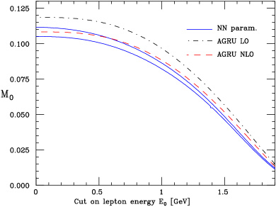
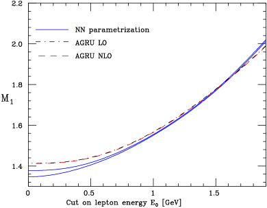
As one example of the applications of the present parametrization of the lepton energy spectrum, in this section our results are compared with the theoretical calculation of Ref. [16] (AGRU). Their formalism allows the computation of moments of different differential distributions from semileptonic B meson decays, with arbitrary kinematical cuts, like the lepton energy spectrum in charmed decays that is analyzed in the present work. In particular their computation of the lepton energy spectrum will be studied, which they define as

$$N_{k}\equiv\frac{1}{\Gamma_{\mathrm{LO}}}\int_{E_{0}}^{E_{\max}}dE_{l}dq^{2}dr\tilde{E}_{l}^{k}\frac{d^{3}\Gamma}{dE_{l}drdq^{2}}\ ,$$ (40)

with $\tilde{E}\equiv E/m_{b}$, and where the leading order partonic semileptonic decay rate $\Gamma_{\mathrm{LO}}$ is given by

$$\Gamma_{\mathrm{LO}}=\Gamma_{0}|V_{cb}|^{2}z_{0}(\rho)\ ,$$ (41)

where $\rho\equiv m_{c}^{2}/m_{b}^{2}$ and the phase space factor is defined in Eq. 12. These moments can be related to the moments as measured experimentally , defined in Eqns. (14- 16), in a straightforward way, for example for the first two moments one has

$$M_{0}=\tau_{B}\Gamma_{0}N_{0},\qquad M_{1}=m_{b}\frac{N_{1}}{N_{0}}\ ,$$ (42)

and similarly for the other moments.

Figure 16: Comparison of the results of Ref. [16] on the partial branching ratio Eq. 14 and the same quantity computed from our parametrization.

Figure 17: Same as Fig. 17 but for first moment, Eq. 15.

Figure 18: Comparison of the results of Ref. [16] on the partial branching ratio Eq. 14 at NLO with associated theoretical uncertainties with the same quantity computed from our parametrization.

Figure 19: Same as Fig. 19 but for first moment, Eq. 15.

Figure 20: Comparison of the results of Ref. [16] on the fourth moment $\overline{M}_{4}(E_{0})$ at NLO with associated theoretical uncertainties with the same quantity computed from our parametrization. Note that this moment has not been measured experimentally.

In Figs. 17 and 17, the results of [16] both at leading order (LO) and at next-to-leading order (NLO) are compared with the moments obtained from our parametrization as a function of the lower cut in the lepton energy $E_{0}$. Comparing results at different perturbative orders is interesting to asses the behaviour of the perturbative expansion. One should take into account in this comparison that the results of [16] are purely perturbative, therefore the difference between the two results could be an indicator of the size of the missing nonperturbative corrections. Another interesting feature is that while for $M_{0}$, the partial branching fraction, the NLO corrections are sizable and bring the theoretical prediction in better agreement with the experimental measurement, for $M_{1}$ (which is the ratio of two perturbative expansions) the size of the perturbative corrections is much smaller.

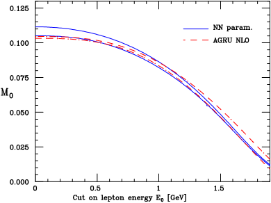
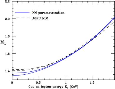
In Figs. 19 and 19 we show similar results as those of Figs. 17 and 17 but this time with an estimation of the theoretical uncertainties associated to the predictions of Ref. [16]. These theoretical uncertainties are obtained by varying the b quark mass $m_{b}$ 100 MeV above and below the central value, and similarly for the strong coupling $\alpha_{s}(m_{b}^{2})$. The known fact that the uncertainties of theoretical predictions grows for large values of the cut in the lepton energy $E_{0}$ is clearly observed in these results. Note that in all cases comparison of theoretical predictions with theoretical measurements can be performed for arbitrary values of the cut in the lepton energy $E_{0}$.

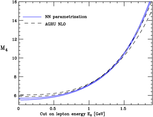
On top of that, in Fig. 20 we compare a quantity that has not been measured, the fourth moment of the spectrum, defined as

$$\widetilde{M}_{4}\left(E_{0}\right)=\frac{L_{4}(E_{0},0)}{L_{0}(E_{0},0)}=m_{b}^{4}\frac{N_{4}(E_{0})}{N_{0}(E_{0})}\ .$$ (43)

We observe good agreement for the theoretical prediction and the experimental data in the region $0.8\leq E_{0}\leq 1.5$ GeV with rather small uncertainties in both cases. It can also be seen that for $E_{0}\geq 1.5$ GeV the theoretical uncertainty for this moment grows while the experimental uncertainty remains rather small, which implies that theoretical uncertainties should be reduced at least by a factor of 2 or 3 to be able to perform quantitative comparisons with experimental data for moments with large cut in the lepton energy. Note therefore that the results in this section imply quantitatively how the uncertainties in theoretical predictions should be reduced to obtain a meaningful comparison with experimental data, for example for moments with large cuts in the lepton energy $E_{0}$.

A more general comparison with theoretical predictions should include also the known nonperturbative power corrections up to order $\mathcal{O}(1/m_{b}^{3})$ to the expressions for the moments of the spectrum, since in this case the difference of the theoretical results from our parametrization would indicate the size of the missing unknown corrections, both perturbative and nonperturbative. A more detailed study of this point, together with an analysis of possible violations of local quark-hadron duality, is left for future work.

The analysis presented in this section is a particular example of how the technique introduced in this work allows a more general comparison of theoretical predictions with experimental data. For example, current experiments do not measure the leptonic moments with $E_{0}>1.5$ GeV, since it is argued that the corresponding theoretical prediction has large uncertainties. If in the future this theoretical error in the computation of leptonic moments with large values for the cut $E_{0}$ is reduced, comparison with experimental results can be straightforward, if one computes these moments from the neural network parametrization of the lepton spectrum, which encodes all the information on available experimental data.

7 Determination of $m_{b}^{1S}$ and $\lambda_{1}$

As another application of our parametrization of the lepton energy spectrum, it will be used to determine the b quark mass $m_{b}^{1S}$ from the experimental data using a novel strategy. To this purpose the technique of Ref. [14] will be used, which consists on the minimization of the size of higher order corrections to obtain sets of moments of the lepton energy spectrum which have reduced theoretical uncertainty for the extraction of nonperturbative parameters like $\bar{\Lambda}_{1S}$ and $\lambda_{1}$. Note that the nonperturbative parameter $\bar{\Lambda}_{1S}$ relates the spin-averaged B meson mass $\bar{m}_{B}$ to the 1S scheme b-quark mass $m_{b}^{1S}$,

$$\bar{\Lambda}_{1S}\equiv\bar{m}_{B}-m_{b}^{1S}\ .$$ (44)

The 1S scheme b-quark mass is related to the standard b quark pole mass $m_{b}^{\mathrm{pole}}$ by a perturbative relation,

$$m_{b}^{1S}=m_{b}^{\mathrm{pole}}\left(1+\sum_{k=2}^{\infty}C_{k}\alpha_{s}\left(m_{b}\right)^{k}\right)\ .$$ (45)

The use of heavy quark masses, like the 1S mass or the MSbar mass, which are not infrared sensitive, is compulsary to avoid the uncertainties assciated to the renormalon divergence of some infrared sensitive definitions of the heavy quark masses, like the pole mass. The parameter $\lambda_{1}$ that appears in Eq. 2 is related to the the definition of the heavy quark pole masses [20] in the following way,

$$m_{b}^{\mathrm{pole}}-m_{c}^{\mathrm{pole}}=\bar{m}_{B}-\bar{m}_{D}+\lambda_{1}\frac{\bar{m}_{B}-\bar{m}_{D}}{2\bar{m}_{B}\bar{m}_{D}}+\mathcal{O}\left(\frac{1}{\bar{m}_{B}^{2}}\right)\ .$$ (46)

The moments that minimize the impact of the higher order nonperturbative corrections are given by

$$R_{1}\equiv\frac{\int_{1.3}^{E_{\max}}E_{l}^{1.4}\frac{d\Gamma}{dE_{l}}dE_{l}}{\int_{1}^{E_{\max}}E_{l}\frac{d\Gamma}{dE_{l}}dE_{l}}\ ,$$ (47)

and

$$R_{2}\equiv\frac{\int_{1.4}^{E_{\max}}E_{l}^{1.7}\frac{d\Gamma}{dE_{l}}dE_{l}}{\int_{0.8}^{E_{\max}}E_{l}^{1.2}\frac{d\Gamma}{dE_{l}}dE_{l}}\ .$$ (48)

The full expression for this moments in terms of heavy-quark non-perturbative parameters can be found in Ref. [14], where in terms or their original notation one has $R_{1}\equiv R_{a}^{(1)}$ and $R_{2}\equiv R_{a}^{(2)}$. These leptonic moments $R_{1}$ and $R_{2}$ depend on 9 nonperturbative parameters, up to $\mathcal{O}(1/m_{b}^{3})$: $\bar{\Lambda}_{1S}$, $\lambda_{1}$ and $\lambda_{2}$, and six matrix elements, $\rho_{1},\rho_{2},\tau_{1},\tau_{2},\tau_{3}$ and $\tau_{4}$, that contribute at order $1/m_{b}^{3}$ in the heavy quark expansion. Present data is not capable of a determination of all these matrix elements. For the $\lambda_{2}$ parameter we use

$$\lambda_{2}\left(m_{b}\right)=\frac{m_{b}^{2}\Delta m_{B}-m_{c}^{2}\Delta m_{D}}{2\left(m_{b}-\kappa m_{c}\right)}\ ,$$ (49)

while to to asses the contribution of the $\mathcal{O}\left(1/m_{b}^{3}\right)$ parameters, the matrix elements $\tau_{i}$ are varied between $\pm\left(500~{}\mathrm{MeV}\right)^{3}$ (the expected size of this matrix elements), $\rho_{1}$ between 0 and $\left(500~{}\mathrm{MeV}\right)^{3}$ (since from the vacuum saturation approximation one knows that $\rho_{1}\geq 0$), and for the matrix element $\rho_{2}$ one uses the relation from the power corrections to the meson mass splittings [20, 36],

$$\rho_{2}=\tau_{2}+\tau_{4}+\frac{m_{b}m_{c}\left[\kappa m_{b}\Delta m_{B}-m_{c}\Delta m_{D}\right]}{2\left(m_{b}-\kappa m_{c}\right)}\ ,$$ (50)

where we have defined

$$\kappa=\left(\frac{\alpha_{s}(m_{c})}{\alpha_{s}(m_{b})}\right)^{3/\beta_{0}},\qquad\Delta m_{Q}=m_{Q*}-m_{Q}\ ,$$ (51)

and where $\kappa$ account for the scale dependence of the parameter $\lambda_{2}$.

The most relevant feature of these leptonic moments $R_{1}$ and $R_{2}$ is that they have non-integer powers and to the best of our knowledge have not been yet experimentally measured, at least in a publised form. Therefore, the values of $R_{1}$ and $R_{2}$ that will be used in this analysis are extracted from our neural network parametrization of the lepton spectrum, which allows the computation of arbitrary moments, together with their associated error and correlation. Let us recall that the central values are determined as

$$\left\langle R_{1}^{(\mathrm{net})}\right\rangle=\frac{1}{N_{\mathrm{rep}}}\sum_{k=1}^{N_{\mathrm{rep}}}R_{1}^{(\mathrm{net})(k)},\qquad R_{1}^{(\mathrm{net})(k)}=\frac{\int_{1.3}^{E_{\max}}E_{l}^{1.4}\frac{d\Gamma^{(\mathrm{net})(k)}}{dE_{l}}(E_{l})dE_{l}}{\int_{1}^{E_{\max}}E_{l}\frac{d\Gamma^{(\mathrm{net})(k)}}{dE_{l}}(E_{l})dE_{l}}\ ,$$ (52)

and similarly for $R_{2}$, and the error and the correlation of the moments $R_{1}$ and $R_{2}$ are computed in the standard way. The following values for the moments with the associated errors and their correlation are obtained,

$$R_{1}^{(\mathrm{net})}=1.017\pm 0.003,\quad R_{2}^{(\mathrm{net})}=0.938\pm 0.004,\quad\rho_{12}=0.94\ ,$$ (53)

that as expected are highly correlated. Then to determine the nonperturbative parameters $\Lambda_{1S}$ and $\lambda_{1}$ the associated $\chi^{2}_{\mathrm{fit}}$ is minimized,

$$\chi^{2}_{\mathrm{fit}}=\sum_{i,j=1}^{2}\left(R_{i}^{(\mathrm{net})}-R_{i}^{(\mathrm{th})}\right)\left(\mathrm{cov}^{-1}\right)_{ij}\left(R_{j}^{(\mathrm{net})}-R_{j}^{(\mathrm{th})}\right)\ ,$$ (54)

where $\mathrm{cov}^{-1}_{ij}$ is the inverse of the covariance matrix associated to the two moments $R_{1}^{(\mathrm{net})}$ and $R_{2}^{(\mathrm{net})}$, and $R_{i}^{(\mathrm{th})}\left(\bar{\Lambda}_{1S},\lambda_{1}\right)$ is the theoretical prediction for these moments as a function of the two nonperturbative parameters [14].

Once the values of $\bar{\Lambda}_{1S}$ and $\lambda_{1}$ have been determined from the minimization of Eq. 54, if one uses for the spin averaged B meson mass the values for the current world average [32]

$$\bar{m}_{B}=\frac{1}{4}\left(m_{P}+3m_{V}\right)=\left(5.3135\pm 0.0008\right)~{}\mathrm{GeV}\ ,$$ (55)

then using the extracted value of $\bar{\Lambda}_{1S}$,

$$\bar{\Lambda}_{1S}=\left(0.47\pm 0.14^{\mathrm{exp}}\pm 0.05^{\mathrm{th}}\right)~{}\mathrm{GeV}\,$$ (56)

one obtains for the b quark mass $m_{b}^{1S}$ mass in the 1S scheme the following value:

$$m_{b}^{1S}=\bar{m}_{B}-\bar{\Lambda}_{1S}=\left(4.84\pm 0.14^{\mathrm{exp}}\pm 0.05^{\mathrm{th}}\right)~{}\mathrm{GeV}=\left(4.84\pm 0.15^{\mathrm{tot}}\right)~{}\mathrm{GeV}\ ,$$ (57)

From the above results one observes that the dominant source of uncertainty is the experimental uncertainty, that is, the uncertainty associated to our parametrization of the lepton energy spectrum. This determination of the b quark mass is consistent with determinations from other analysis. The b quark mass has been determined using different techniques, like the sum rule approach, using either non-relativistic [34, 35, 37, 38] or relativistic [39, 40] sum rules, global fits of moments of differential distributions in B decays, [41, 33, 28], the renormalon analysis of Ref. [42], and several other methods related to heavy-quarkonium physics [43, 44] (see [45] for a review). To compare our results with some of the above references, it is useful to relate the $m^{1S}_{b}$ mass to the MS-bar $\bar{m}_{b}\left(\bar{m}_{b}\right)$ mass [35, 46], and once the conversion is performed the value

$$\bar{m}_{b}\left(\bar{m}_{b}\right)=\left(4.31\pm 0.15^{\mathrm{tot}}\right)~{}\mathrm{GeV}\ ,$$ (58)

is obtained, where we have used $\alpha_{s}(M_{Z}^{2})=0.1182$ and included perturbative corrections up to two loops. It turns out that our determination of $m^{1S}_{b}$ is not competitive with respect to other determinations since only two moments, $R_{1}$ and $R_{2}$ are used to constrain the nonperturbative parameters in the fit. Note therefore that the relatively large error in the extraction of $\bar{m}_{b}\left(\bar{m}_{b}\right)$ are not due to large uncertainties in our parametrization of the lepton energy spectrum, which are the same than experimental data, but rather from the use of a reduced set of moments in the fit. Note also that the motivation to perform this determination of $\bar{m}_{b}\left(\bar{m}_{b}\right)$ is to show how the neural network parametrization constructed in this work allows a more general comparison of experimental data with theoretical predictions, in this case allowing to use moments with fractional index with their errors and correlations, which have not been measured directly, at least in a published form. The inclusion of additional moments would therefore constrain more the nonperturbative parameters and reduce the experimental uncertainty associated to them.

For the nonperturbative parameter $\lambda_{1}$ the following value is obtained

$$\lambda_{1}=\left(-0.16\pm 0.14^{\mathrm{exp}}\pm 0.05^{\mathrm{th}}\right)~{}\mathrm{GeV^{2}}=\left(-0.16\pm 0.15^{\mathrm{tot}}\right)~{}\mathrm{GeV^{2}}\ .$$ (59)

As in the determination of $\bar{\Lambda}_{1S}$ it can be seen that the theoretical uncertainties are smaller than the experimental ones, which are the dominant ones. Our result for the parameter $\lambda_{1}$ is consistent with other extractions in the context of global fits of B decay data [41, 33], but again not competitive due to the large experimental uncertainties.

In summary, a determination of $m^{1S}_{b}$ and $\lambda_{1}$ has been obtained from our neural network parametrization in a way that was not directly possible from the available experimental data. However, it turns out that the experimental uncertainties in the present determination do not allow these results to be competitive with those from other determinations using different techniques, even if in this approach the theoretical uncertainties where minimized.

8 Conclusions and outlook

This works presents a determination of the probability density in the space of the lepton energy spectra from semileptonic B meson decays, based on the latest available data from the Babar, Belle and Cleo collaborations, that makes use of a combination of Monte Carlo techniques and neural networks with results in an unbiased parametrization with faithful estimation of the uncertainties. In addition, this work shows the implementation of a well definite strategy to reconstruct functions with uncertainties when the only available experimental information comes through convolutions of these functions. Moreover, in our formalism the implementation of arbitrary theoretical constraints can be done in a consistent and unbiased way.

As a byproduct of our analysis, with our parametrization of the lepton spectrum, the nonperturbative parameters $\bar{\Lambda}_{1S}$ and $\lambda_{1}$ have been extracted in a way that minimizes the theoretical uncertainties. For the b quark mass in the $1S$ scheme the result $m_{b}^{1S}=\bar{m}_{B}-\bar{\Lambda}_{1S}=\left(4.84\pm 0.16^{\mathrm{exp}}\pm 0.05^{\mathrm{th}}\right)~{}\mathrm{GeV}$ has been obtained. Although this application demonstrates the flexibility of our approach to allow a more general comparison of data with theoretical predictions, it turns out that the use of a reduced set of non-integer moments implies that uncertainties are rather large to make this determination competitive with those from global fits of moments of B meson decay distributions [41, 33, 28], which include additional moments. A reevaluation of $m_{b}^{1S}$ from our neural network parametrization of the lepton energy spectrum with a larger set of moments will be studied in a following work.

The number of possible applications of this strategy to other problems in B physics is rather large. For example, the inclusion of hadronic moments would allow a parametrization of the double differential decay rate

$$\frac{d^{2}\Gamma}{dE_{l}dr}(E_{l},r)\equiv\int dq^{2}\frac{d^{3}\Gamma}{dq^{2}dE_{l}dr}\ ,$$ (60)

in terms of a neural network with two inputs. From this two-dimensional spectrum the hadronic invariant mass moments, as have been recently measured by Babar [47] and Belle [48], would be computed as

$$H_{n}(E_{0},\mu)\equiv\int_{E_{0}}^{E_{\max}}dE_{l}\int_{0}^{M_{B}/2}dr(r-\mu)^{n}\frac{d^{2}\Gamma}{dE_{l}dr}(E_{l},r)\ .$$ (61)

In this case both the training and the implementation of the kinematical constraints is rather more complicated, since one has to parametrize a two-dimensional surface.

The charmless decay channel, $B\to X_{u}l\nu$ would be also interesting to analyze, since it has received a lot of theoretical attention recently, specially in the context of effective field theories, see for example Refs. [49, 50, 51, 52, 53, 54] and references therein. However, this mode is more challenging to measure due to large backgrounds. Another interesting application would be to estimate with our technique the issue of the parametrization dependence of the form factor of the $B\to\pi l\nu$ exclusive channel, as discussed in Ref. [55].

A process that is closely related to the semileptonic decays is the analysis of the photon energy spectrum in $B\to X_{s}\gamma$ decays [57, 58]. This process has also been recently measured with good accuracy at the B factories, by Babar [59] and by Belle [60]. The strategy to be followed in this process would be very similar to that of the present work, since the experimental information has the same form.

Finally one can use the neural network strategy to construct a parametrization of the shape function $S(k)$ of the B meson, a universal characteristic of the B meson that governs inclusive decay spectra in processes with massless partons in the final state, as extracted from the $B\to X_{s}\gamma$ and $B\to X_{u}l\nu$ decay modes. In this case there exist more theoretical information on its shape. For example, at tree level its moments

$$A_{n}\equiv\int dkk^{n}S(k)$$ (62)

have to satisfy $A_{0}=1,A_{1}=0$ and $A_{2}=\mu_{\pi}^{2}/3$. At higher orders these relations are theoretically more controversial [61, 62]. Since the uncertainty from the extraction of $S(k)$ is the dominant source of theoretical uncertainty in some CKM matrix elements extraction, it would therefore be interesting to estimate again this uncertainty with the technique presented in this work, since in the current approach [63] the shape function uncertainties are estimated in a rather crude way, with a combination of different functional forms compatible with the theoretical constraints. The application of the techniques introduced in this work to obtain an unbiased parametrization of the B meson shape function with a faithful estimation of its uncertainties from experimental data will be discussed in a forthcoming publication [12].

The set of trained neural networks that represents the probability measure in the space of differential lepton energy spectra, together with the driver program and a user manual are available from the author.

Appendix A Details of the neural network training

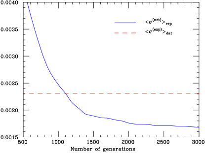
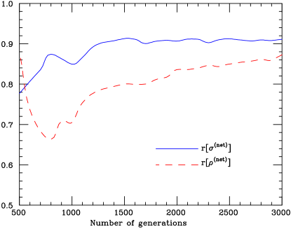
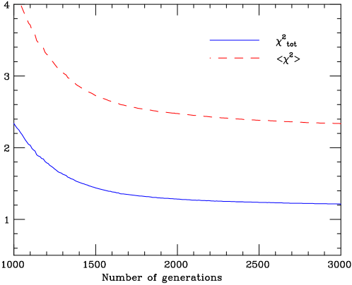
In this Appendix a more detailed statistical analysis of the parametrization of the lepton energy spectrum is performed. To understand better the process of neural network training it is interesting to analyze the evolution of the different statistical estimators, as defined in Appendix B, with respect to the number of generations, that is, with respect of the training length. In fig. 21 the evolution of $\chi^{2}_{\mathrm{tot}}$ and of $\left\langle\chi^{2}\right\rangle$ computed from the trained replica sample can be observed. Note that at the end of the training $\chi^{2}_{\mathrm{tot}}\sim 1$ and $\left\langle\chi^{2}\right\rangle\sim 2$, as expected. Note also that the fit has reached convergence with the $\chi^{2}_{\mathrm{tot}}$ profile is very flat for a large number of generations.

This can be repeated for other statistical estimators, like for example the average spread of the data points as computed from the neural network ensemble, Fig. 23, defined in Appendix B, which is to be compared with the same quantity computed from the experimental data, $\sigma_{i}^{(\mathrm{exp})}$. The fact that one has error reduction, as has been explained in [7], is the sign that the network has found an underlying law to the experimental data, in this case the lepton energy spectrum.

Other relevant estimator is the so-called scatter correlations of the spread of the points (see Fig. 23). The scatter correlation indicates the size of the spread of data around a straight line. Specifically $r\left[\sigma^{(\mathrm{net})}\right]=1$ implies that $\left\langle\sigma_{i}^{(\mathrm{net})}\right\rangle$ is proportional to $\sigma_{i}^{(\mathrm{exp})}$. One can define similarly a scatter correlation for the net correlation $\rho_{ij}^{(\mathrm{net})}$, also represented in Fig. 23 for the Babar experimental data. One observes that when the training ends both values of $r$ are close to 1, a sign that errors and correlations are faithfully reproduced.

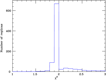
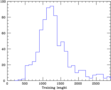
Another relevant estimator of the goodness of the fit is the distribution of both $\chi^{2(k)}$ and of the training lengths over the replica sample, figures 25, and 25. The distribution of $\chi^{2(k)}$ over the replica sample should be rather peaked around $\left\langle\chi^{2}\right\rangle$, because the opposite case would mean that the averaged result is obtained as a combination very good fits with very bad fits (in the sense of fits with very large $\chi^{2}$). It can be observed in Figure 25 that indeed our distribution is very peaked around the average. On the other hand, the distribution of training lenghts, Fig. 25, has to be smooth and it cannot be peaked at $N_{\mathrm{gen}}$, because if a too large fraction of the nets never reach the condition $\chi^{2(k)}\leq\chi^{2}_{\mathrm{stop}}$ then effectively one is stopping the training after a fixed number of generations regardless of the value of the $\chi^{2(k)}$ of the trained replica. It can be seen that only $\sim 20\%$ of the trained replicas do not reach $\chi^{2}_{\mathrm{stop}}$, which is an acceptable fraction.

Figure 21: Total $\chi^{2}_{\mathrm{tot}}$, Eq. 74 of the replica sample, compared with average error, $\left\langle\chi^{2}\right\rangle$, Eq. 75.

Figure 22: Average error of the data points as computed from the neural network sample, Eq. 64, as compared with the experimental value.

Figure 23: The scatter correlations, Eq. 73 as a function of the lenght of the training, for the Babar experimental data.

Figure 24: Distribution of $\chi^{2}$ over the sample of trained replicas.

Figure 25: Distribution of training lenghts over the sample of trained replicas.

Appendix B Statistical estimators

In this appendix the statistical estimators that are used to asses the quality of both the Monte Carlo replica generation and the neural network training are described. The superscripts $(\mathrm{dat})$, $(\mathrm{art})$ and $(\mathrm{net})$ refer respectively to the original data, to the $N_{\mathrm{rep}}$ Monte Carlo replicas of the data, and to the $N_{\mathrm{rep}}$ neural networks. The subscripts $\mathrm{rep}$ and $\mathrm{dat}$ refer respectively to whether averages are taken by summing over all replicas or over all data.

• Replica averages

  • Average over the number of replicas for each experimental point $i$

    $$\left\langle M_{i}^{(\mathrm{art})}\right\rangle_{\mathrm{rep}}=\frac{1}{N_{\mathrm{rep}}}\sum_{k=1}^{N_{\mathrm{rep}}}M_{i}^{(\mathrm{art})(k)}\ .$$ (63)

  • Associated variance

    $$\sigma_{i}^{(\mathrm{art})}=\sqrt{\left\langle\left(M_{i}^{(\mathrm{art})}\right)^{2}\right\rangle_{\mathrm{rep}}-\left\langle M_{i}^{(\mathrm{art})}\right\rangle^{2}_{\mathrm{rep}}}\ .$$ (64)

  • Associated covariance

    $$\rho_{ij}^{(\mathrm{art})}=\frac{\left\langle M_{i}^{(\mathrm{art})}M_{j}^{(\mathrm{art})}\right\rangle_{\mathrm{rep}}-\left\langle M_{i}^{(\mathrm{art})}\right\rangle_{\mathrm{rep}}\left\langle M_{j}^{(\mathrm{art})}\right\rangle_{\mathrm{rep}}}{\sigma_{i}^{(\mathrm{art})}\sigma_{j}^{(\mathrm{art})}}\ .$$ (65)

    $$\mathrm{cov}_{ij}^{(\mathrm{art})}=\rho_{ij}^{(\mathrm{art})}\sigma_{i}^{(\mathrm{art})}\sigma_{j}^{(\mathrm{art})}\ .$$ (66)

  • Percentage error on central values over the $N_{\mathrm{dat}}$ data points.

    $$\left\langle PE\left[\left\langle M^{(\mathrm{art})}\right\rangle_{\mathrm{rep}}\right]\right\rangle_{\mathrm{dat}}=\frac{1}{N_{\mathrm{dat}}}\sum_{i=1}^{N_{\mathrm{dat}}}\left[\frac{\left\langle M_{i}^{(\mathrm{art})}\right\rangle_{\mathrm{rep}}-M_{i}^{(\mathrm{exp})}}{M_{i}^{(\mathrm{exp})}}\right]\ .$$ (67)

    We define analogously $\left\langle PE\left[\left\langle\sigma^{(\mathrm{art})}\right\rangle_{\mathrm{rep}}\right]\right\rangle_{\mathrm{dat}}$.

  • Scatter correlation:

    $$r\left[M^{(\mathrm{art})}\right]=\frac{\left\langle M^{(\mathrm{exp})}\left\langle M^{(\mathrm{art})}\right\rangle_{\mathrm{rep}}\right\rangle_{\mathrm{dat}}-\left\langle M^{(\mathrm{exp})}\right\rangle_{\mathrm{dat}}\left\langle\left\langle M^{(\mathrm{art})}\right\rangle_{\mathrm{rep}}\right\rangle_{\mathrm{dat}}}{\sigma_{s}^{(\mathrm{exp})}\sigma_{s}^{(\mathrm{art})}}\,$$ (68)

    where the scatter variances are defined as

    $$\sigma_{s}^{(\mathrm{exp})}=\sqrt{\left\langle\left(M^{(\exp)}\right)^{2}\right\rangle_{\mathrm{dat}}-\left(\left\langle M^{(\exp)}\right\rangle_{\mathrm{dat}}\right)^{2}}\,$$ (69)

    $$\sigma_{s}^{(\mathrm{art})}=\sqrt{\left\langle\left(\left\langle M^{(\mathrm{art})}\right\rangle_{\mathrm{rep}}\right)^{2}\right\rangle_{\mathrm{dat}}-\left(\left\langle\left\langle M^{(\mathrm{art})}\right\rangle_{\mathrm{rep}}\right\rangle_{\mathrm{dat}}\right)^{2}}\ .$$ (70)

    We define analogously $r\left[\sigma^{(\mathrm{art})}\right]$, $r\left[\rho^{(\mathrm{art})}\right]$ and $r\left[\mathrm{cov}^{(\mathrm{art})}\right]$. Note that the scatter correlation and scatter variance are not related to the variance and correlation Eqs. 64-66.

  • Average variance:

    $$\left\langle\sigma^{(\mathrm{art})}\right\rangle_{\mathrm{dat}}=\frac{1}{N_{\mathrm{dat}}}\sum_{i=1}^{N_{\mathrm{dat}}}\sigma_{i}^{(\mathrm{art})}\ .$$ (71)

    We define analogously $\left\langle\rho^{(\mathrm{art})}\right\rangle_{\mathrm{dat}}$ and $\left\langle\mathrm{cov}^{(\mathrm{art})}\right\rangle_{\mathrm{dat}}$, as well as the corresponding experimental quantities.

• Neural network averages

  • Mean variance and percentage error on central values over the $N_{\mathrm{dat}}$ data points.

    $$\left\langle PE\left[\left\langle M^{(\mathrm{net})}\right\rangle_{\mathrm{rep}}\right]\right\rangle_{\mathrm{dat}}=\frac{1}{N_{\mathrm{dat}}}\sum_{i=1}^{N_{\mathrm{dat}}}\left[\frac{\left\langle M_{i}^{(\mathrm{net})}\right\rangle_{\mathrm{rep}}-M_{i}^{(\mathrm{exp})}}{M_{i}^{(\mathrm{exp})}}\right]\ .$$ (72)

  • We define analogously percentage errors on the correlation and covariance.

  • Scatter correlation

    $$r\left[M^{(\mathrm{net})}\right]=\frac{\left\langle M^{(\mathrm{exp})}\left\langle M^{(\mathrm{net})}\right\rangle_{\mathrm{rep}}\right\rangle_{\mathrm{dat}}-\left\langle M^{(\mathrm{exp})}\right\rangle_{\mathrm{dat}}\left\langle\left\langle M^{(\mathrm{net})}\right\rangle_{\mathrm{rep}}\right\rangle_{\mathrm{dat}}}{\sigma_{s}^{(\mathrm{exp})}\sigma_{s}^{(\mathrm{net})}}\ .$$ (73)

    We define analogously $\left\langle\rho^{(\mathrm{net})}\right\rangle_{\mathrm{dat}}$ and $\left\langle\mathrm{cov}^{(\mathrm{net})}\right\rangle_{\mathrm{dat}}$.

On top of these, one has also to define the estimators that measure the global quality of the fit, namely the total error

$$\chi^{2}_{\mathrm{tot}}=\frac{1}{N_{\mathrm{dat}}}\sum_{i=1}^{N_{\mathrm{dat}}}\frac{\left(M_{i}^{(\exp)}-\left\langle M_{i}^{(\mathrm{net})}\right\rangle_{\mathrm{rep}}\right)^{2}}{\sigma_{\mathrm{tot},i}^{2}}\ ,$$ (74)

and the average error over the replica sample,

$$\left\langle\chi^{2}\right\rangle=\frac{1}{N_{\mathrm{rep}}}\sum_{i=k}^{N_{\mathrm{rep}}}\frac{1}{N_{\mathrm{dat}}}\sum_{i=1}^{N_{\mathrm{dat}}}\frac{\left(M_{i}^{(\mathrm{art})(k)}-M_{i}^{(\mathrm{net})(k))}\right)^{2}}{\sigma_{\mathrm{tot},i}^{2}}\ .$$ (75)

On general grounds [7] one expects the relation $\left\langle\chi^{2}\right\rangle\sim\chi^{2}_{\mathrm{tot}}+1$ to hold, and indeed this is the case as can be seen in Tables 4 and 5.

References

- [1] Hewett, J. et al., The discovery potential of a super b factory., hep-ph/0503261.
- [2] P. Gambino and N. Uraltsev, Moments of semileptonic b decay distributions in the expansion, Eur. Phys. J. C34 (2004) 181–189, [hep-ph/0401063].
- [3] M. Trott, Improving extractions of and the b quark mass from semileptonic inclusive b decay, Int. J. Mod. Phys. A19 (2004) 5493–5500, [hep-ph/0409186].
- [4] P. Gambino, Semileptonic and radiative b decays circa 2005, hep-ph/0510085.
- [5] J. Chay, H. Georgi, and B. Grinstein, Lepton energy distributions in heavy meson decays from qcd, Phys. Lett. B247 (1990) 399–405.
- [6] I. I. Y. Bigi, M. A. Shifman, N. G. Uraltsev, and A. I. Vainshtein, QCD predictions for lepton spectra in inclusive heavy flavor decays, Phys. Rev. Lett. 71 (1993) 496–499, [hep-ph/9304225].
- [7] S. Forte, L. Garrido, J. I. Latorre, and A. Piccione, Neural network parametrization of deep-inelastic structure functions, JHEP 05 (2002) 062, [hep-ph/0204232].
- [8] NNPDF Collaboration, L. Del Debbio, S. Forte, J. I. Latorre, A. Piccione, and J. Rojo, Unbiased determination of the proton structure function with faithful uncertainty estimation, hep-ph/0501067.
- [9] J. Rojo and J. I. Latorre, Neural network parametrization of spectral functions from hadronic tau decays and determination of qcd vacuum condensates, JHEP 01 (2004) 055, [hep-ph/0401047].
- [10] NNPDF Collaboration, L. Del Debbio, S. Forte, J. I. Latorre, A. Piccione, and J. Rojo, The neural network approach to parton fitting: The nonsinglet case.
- [11] NNPDF Collaboration, J. Rojo, L. Del Debbio, S. Forte, J. I. Latorre, and A. Piccione, The neural network approach to parton fitting, hep-ph/0505044.
- [12] G. Ossola, A. Piccione, and J. Rojo, Neural network parametrization of the B meson shape function, In preparation.
- [13] M. Dittmar et al., Parton distributions: Summary report for the HERA - LHC workshop, hep-ph/0511119.
- [14] C. W. Bauer and M. Trott, Reducing theoretical uncertainties in and , Phys. Rev. D67 (2003) 014021, [hep-ph/0205039].
- [15] M. Trott, Improving extractions of and from the hadronic invariant mass moments of semileptonic inclusive B decay, Phys. Rev. D70 (2004) 073003, [hep-ph/0402120].
- [16] V. Aquila, P. Gambino, G. Ridolfi, and N. Uraltsev, Perturbative corrections to semileptonic b decay distributions, Nucl. Phys. B719 (2005) 77–102, [hep-ph/0503083].
- [17] M. Jezabek and J. H. Kuhn, Lepton spectra from heavy quark decay, Nucl. Phys. B320 (1989) 20.
- [18] M. Gremm and I. Stewart, Order alpha(s)**2 beta(0) correction to the charged lepton spectrum in b —¿ c l anti-nu/l decays, Phys. Rev. D55 (1997) 1226–1232, [hep-ph/9609341].
- [19] A. V. Manohar and M. B. Wise, Inclusive semileptonic b and polarized decays from QCD, Phys. Rev. D49 (1994) 1310–1329, [hep-ph/9308246].
- [20] M. Gremm and A. Kapustin, Order corrections to inclusive semileptonic B decay, Phys. Rev. D55 (1997) 6924–6932, [hep-ph/9603448].
- [21] D. Benson, I. I. Bigi, T. Mannel, and N. Uraltsev, Imprecated, yet impeccable: On the theoretical evaluation of , Nucl. Phys. B665 (2003) 367–401, [hep-ph/0302262].
- [22] BABAR Collaboration, B. Aubert et al., Measurement of the electron energy spectrum and its moments in inclusive decays, Phys. Rev. D69 (2004) 111104, [hep-ex/0403030].
- [23] H. F. A. Group et al., Averages of B hadron properties at the end of 2005, hep-ex/0603003.
- [24] Belle Collaboration, Moments of the electron energy spectrum in decays at belle, hep-ex/0508056.
- [25] CLEO Collaboration, A. H. Mahmood et al., Measurement of the B-meson inclusive semileptonic branching fraction and electron energy moments, Phys. Rev. D70 (2004) 032003, [hep-ex/0403053].
- [26] CDF Collaboration, D. Acosta et al., Measurement of the moments of the hadronic invariant mass distribution in semileptonic B decays, Phys. Rev. D71 (2005) 051103, [hep-ex/0502003].
- [27] BABAR Collaboration, B. Aubert et al., Determination of the branching fraction for decays and of Vcb from hadronic mass and lepton energy moments, Phys. Rev. Lett. 93 (2004) 011803, [hep-ex/0404017].
- [28] O. Buchmueller and H. Flaecher, Fits to moment measurements from and decays using heavy quark expansions in the kinetic scheme, hep-ph/0507253.
- [29] Y. A. Kanev, Application of neural networks and genetic algorithms in high-energy physics, PhD. Thesis, UMI-99-05968.
- [30] B. C. Allanach, D. Grellscheid, and F. Quevedo, Genetic algorithms and experimental discrimination of susy models, JHEP 07 (2004) 069, [hep-ph/0406277].
- [31] J. C. Collins and J. Pumplin, Tests of goodness of fit to multiple data sets, hep-ph/0105207.
- [32] Particle Data Group Collaboration, S. Eidelman et al., Review of particle physics, Phys. Lett. B592 (2004) 1.
- [33] DELPHI Collaboration, J. , Abdallah et al., Determination of heavy quark non-perturbative parameters from spectral moments in semileptonic b decays, hep-ex/0510024.
- [34] A. H. Hoang, Bottom quark mass from upsilon mesons, Phys. Rev. D59 (1999) 014039, [hep-ph/9803454].
- [35] A. H. Hoang, 1S and MSbar bottom quark masses from upsilon sum rules, Phys. Rev. D61 (2000) 034005, [hep-ph/9905550].
- [36] C. W. Bauer, Z. Ligeti, M. Luke, and A. V. Manohar, B decay shape variables and the precision determination of and , Phys. Rev. D67 (2003) 054012, [hep-ph/0210027].
- [37] M. Beneke and A. Signer, The bottom MSbar quark mass from sum rules at next-to- next-to-leading order, Phys. Lett. B471 (1999) 233–243, [hep-ph/9906475].
- [38] A. Pineda and A. Signer, Renormalization group improved sum rule analysis for the bottom quark mass, hep-ph/0601185.
- [39] J. H. Kuhn and M. Steinhauser, Determination of and heavy quark masses from recent measurements of , Nucl. Phys. B619 (2001) 588–602, [hep-ph/0109084].
- [40] G. Corcella and A. H. Hoang, Uncertainties in the MSbar bottom quark mass from relativistic sum rules, Phys. Lett. B554 (2003) 133–140, [hep-ph/0212297].
- [41] C. W. Bauer, Z. Ligeti, M. Luke, A. V. Manohar, and M. Trott, Global analysis of inclusive B decays, Phys. Rev. D70 (2004) 094017, [hep-ph/0408002].
- [42] A. Pineda, Determination of the bottom quark mass from the system, JHEP 06 (2001) 022, [hep-ph/0105008].
- [43] N. Brambilla, Y. Sumino, and A. Vairo, Quarkonium spectroscopy and perturbative QCD: A new perspective, Phys. Lett. B513 (2001) 381–390, [hep-ph/0101305].
- [44] N. Brambilla, Y. Sumino, and A. Vairo, Quarkonium spectroscopy and perturbative qcd: Massive quark loop effects, Phys. Rev. D65 (2002) 034001, [hep-ph/0108084].
- [45] N. Brambilla et al., Heavy quarkonium physics, hep-ph/0412158.
- [46] A. H. Hoang, Bottom quark mass from upsilon mesons: Charm mass effects, hep-ph/0008102.
- [47] BABAR Collaboration, B. Aubert et al., Measurements of moments of the hadronic mass distribution in semileptonic B decays, Phys. Rev. D69 (2004) 111103, [hep-ex/0403031].
- [48] BELLE Collaboration, K. Abe et al., Moments of the hadronic mass spectrum in inclusive semileptonic B decays at belle, hep-ex/0408139.
- [49] F. De Fazio and M. Neubert, decay distributions to order , JHEP 06 (1999) 017, [hep-ph/9905351].
- [50] P. Gambino, G. Ossola, and N. Uraltsev, Hadronic mass and moments of charmless semileptonic B decay distributions, JHEP 09 (2005) 010, [hep-ph/0505091].
- [51] B. O. Lange, M. Neubert, and G. Paz, Theory of charmless inclusive B decays and the extraction of , hep-ph/0504071.
- [52] BABAR Collaboration, B. Aubert et al., Measurement of the partial branching fraction for inclusive charmless semileptonic B decays and extraction of , hep-ex/0507017.
- [53] BABAR Collaboration, B. , Aubert et al., Measurement of the inclusive electron spectrum in charmless semileptonic B decays near the kinematic endpoint and determination of —, hep-ex/0509040.
- [54] J. R. Andersen and E. Gardi, Inclusive spectra in charmless semileptonic B decays by dressed gluon exponentiation, hep-ph/0509360.
- [55] T. Becher and R. J. Hill, Comment on form factor shape and extraction of from , hep-ph/0509090.
- [56] A. F. Falk, M. E. Luke, and M. J. Savage, Nonperturbative contributions to the inclusive rare decays and , Phys. Rev. D49 (1994) 3367–3378, [hep-ph/9308288].
- [57] A. L. Kagan and M. Neubert, QCD anatomy of decays, Eur. Phys. J. C7 (1999) 5–27, [hep-ph/9805303].
- [58] J. R. Andersen and E. Gardi, Taming the spectrum by dressed gluon exponentiation, JHEP 06 (2005) 030, [hep-ph/0502159].
- [59] BaBar Collaboration, F. Bucci et al., Results from the babar fully inclusive measurement of , hep-ex/0507001.
- [60] Belle Collaboration, P. Koppenburg et al., An inclusive measurement of the photon energy spectrum in decays, Phys. Rev. Lett. 93 (2004) 061803, [hep-ex/0403004].
- [61] S. W. Bosch, B. O. Lange, M. Neubert, and G. Paz, Factorization and shape-function effects in inclusive B meson decays, Nucl. Phys. B699 (2004) 335–386, [hep-ph/0402094].
- [62] C. W. Bauer and A. V. Manohar, Shape function effects in b –¿ x/s gamma and b –¿ x/u l nu decays, Phys. Rev. D70 (2004) 034024, [hep-ph/0312109].
- [63] I. Bizjak, A. Limosani, and T. Nozaki, Determination of the B quark leading shape function parameters in the shape function scheme using the belle photon energy spectrum, hep-ex/0506057.