CAFPE/70-06

LU TP 06-03

UG-FT/200-06

hep-ph/0601197

January 2006

The $B_{K}$ Kaon Parameter in the Chiral Limit

Johan Bijnens^a), Elvira Gámiz^b) and Joaquim Prades^c)

^a) Department of Theoretical Physics, Lund University

Sölvegatan 14A, S-22362 Lund, Sweden.

^b) Department of Physics & Astronomy, University of Glasgow

Glasgow G12 8QQ, United Kingdom.

^c) Centro Andaluz de Física de las Partículas Elementales (CAFPE) and Departamento de Física Teórica y del Cosmos, Universidad de Granada

Campus de Fuente Nueva, E-18002 Granada, Spain.

We introduce four-point functions in the hadronic ladder resummation approach to large $N_{c}$ QCD Green functions. We determine the relevant one to calculate the $B_{K}$ kaon parameter in the chiral limit. This four-point function contains both the large momenta QCD OPE and the small momenta ChPT at NLO limits, analytically. We get $\hat{B}_{K}^{\chi}=0.38\pm 0.15$. We also give the ChPT result at NLO for the relevant four-point function to calculate $B_{K}$ outside the chiral limit, while the leading QCD OPE is the same as the chiral limit one.

1 Introduction

Indirect kaon CP-violation in the Standard Model (SM) is proportional to the matrix element

$$\langle\overline{K}^{0}|K^{0}\rangle = -iC_{\Delta S=2}\,C(\nu)\,\langle\overline{K^{0}}|\int{\rm d}^{4}y\,Q_{\Delta S=2}(y)|K^{0}\rangle$$ (1)

$$\equiv -iC_{\Delta S=2}\,\frac{16}{3}\,\hat{B}_{K}\,F_{K}^{2}m_{K}^{2}$$

with

$$Q_{\Delta S=2}(x)\equiv 4L^{\mu}(x)L_{\mu}(x)\,;\hskip 14.22636pt2L_{\mu}(x)\equiv\left[\overline{s}\gamma_{\mu}(1-\gamma_{5})d\right](x)\,.$$ (2)

and $C(\nu)$ a Wilson coefficient. $C(\nu)$ and $C_{\Delta S=2}$ are known in perturbative QCD to next-to-leading order (NLO). A review can be found in [1].

The kaon bag parameter, $\hat{B}_{K}$, defined in (1) is an important input for the unitarity triangle analysis and its calculation has been addressed many times in the past. There have been four main QCD-based techniques used to calculate it: QCD-Hadronic Duality [2, 3], three-point function QCD Sum Rules [4], lattice QCD and the $1/N_{c}$ ($N_{c}=$ number of colors) expansion. Recent reviews of the unitarity triangle, where the relevant references for the inputs can be found, are [5]. For recent advances using lattice QCD see [6, 7, 8].

Here, we present a determination of the $\hat{B}_{K}$ parameter at NLO in the $1/N_{c}$ expansion. That the $1/N_{c}$ expansion introduced in [9, 10] would be useful in this regard was first suggested by Bardeen, Buras and Gérard [11] and reviewed by Bardeen in [12, 13]. There one can find most of the references to previous work and applications of this non-perturbative technique.

Work directly related to this work can be found in [14, 15] where a NLO in $1/N_{c}$ calculation of $\hat{B}_{K}$ within and outside the chiral limit was presented. There, the relevant spectral function is calculated at very low energies using Chiral Perturbation Theory (ChPT), at intermediate energies with the extended Nambu-Jona-Lasinio (ENJL) model [16] and at very large energies with the operator product expansion (OPE). The method, including how to deal with the short-distance scheme dependence, has been discussed extensively in [15]. The improvement in the present work is basically in the intermediate energies and the numerical quality of the matching to short distances.

Another calculation of $\hat{B}_{K}$ in the chiral limit at NLO in the $1/N_{c}$ expansion is in [17]. There, the relevant spectral function is saturated by the pion pole and the first rho meson resonance –minimal hadronic approximation (MHA). In [18], the same technique as in [17] was used but including also the effects of dimension eight operators in the OPE of the $\Delta S=2$ Green’s function and adding the first scalar meson resonance to the relevant spectral function. This works differs from that in two aspects. We use our $X$-boson method which allows for an easy identification of the precise scheme used in the hadronic picture by only using currents and densities directly in four dimensions rather than using dimensional regularization throughout. This is a difference in formalism, not in physical content. On the other hand, we use a much more elaborate way to include hadronic states allowing the use of more constraints [19] and thus more resonances than the work of [17, 18]. The hadronic model developed in [19] also includes current quark masses effects and will be used to determine $\hat{B}_{K}$ in the real case [20].

The present manuscript is organized as follows. In Section 2 we collect a few perturbative formulas at NLO in QCD for completeness. Section 3 explains in detail how we derive the value of $\hat{B}_{K}$ from a large $N_{c}$ Green’s function with two densities and two currents. This can be found essentially in [15] but we add here an extra QCD calculation of the short-distance constraint analogous to the equivalent terms in our work on $Q_{7}$ and $Q_{8}$ [21]. QCD is still not solved even at leading order in the $1/N_{c}$ expansion. Therefore, at present, any NLO in $1/N_{c}$ approach to weak matrix elements needs a large $N_{c}$ hadronic model. We present in Section 4 our hadronic model based on a severe approximation to a ladder resummation of QCD as explained in [19]. This model is used at intermediate distances and is the main uncertainty in our approach. Then we discuss the chiral limit results in Section 5. The extension beyond the chiral limit needs more work both at intermediate distances but we include some comments already in Section 6. At short distances, the leading dimension six OPE operator is known and agrees with the chiral one. The last section contains our conclusions and a comparison with other approaches.

Some preliminary results were already presented in [22] and [23].

2 Some perturbative QCD formulas

This section is a compilation of the perturbative QCD coefficients at NLO from [1] needed in our analysis of $\hat{B}_{K}$ and derived in [24].

The coefficients $C(\nu)$ and $C_{\Delta S=2}$ are known in perturbative QCD at next-to-leading order (NLO) in $a\equiv\alpha_{S}/\pi$ in two schemes [1, 24], the ’t Hooft-Veltman (HV) scheme ($\overline{\rm MS}$ subtraction and non-anti-commuting $\gamma_{5}$ in $D\neq 4$) and in the Naive Dimensional Regularization (NDR) scheme ($\overline{\rm MS}$ subtraction and anti-commuting $\gamma_{5}$ in $D\neq 4$). $C_{\Delta S=2}$ collects known functions of the integrated out heavy particle masses and Cabibbo-Kobayashi-Maskawa matrix elements, it can be found in [1, 24]. Its actual form is very important for CKM analysis but not needed here.

The Wilson coefficient $C(\nu)$ is

$$C(\nu)=\left(1+a(\nu)\left[\frac{\gamma_{2}}{\beta_{1}}-\frac{\beta_{2}\gamma_{1}}{\beta_{1}^{2}}\right]\right)\,[\alpha_{s}(\nu)]^{\gamma_{1}/\beta_{1}}\,.$$ (3)

$\gamma_{1}$ is the one-loop $\Delta S=2$ anomalous dimension

$$\gamma_{1}=\frac{3}{2}\left(1-\frac{1}{N_{c}}\right)=1\,.$$ (4)

$\gamma_{2}$ is the two-loop $\Delta S=2$ anomalous dimension [24]

$$\gamma_{2}^{\rm NDR} = -\frac{1}{32}\left(1-\frac{1}{N_{c}}\right)\left[17+\frac{4}{3}(3-n_{f})+\frac{57}{N_{c}}\left(\frac{N_{c}^{2}}{9}-1\right)\right]=-\frac{17}{48}\,,$$

$$\gamma_{2}^{\rm HV} = \gamma_{2}^{\rm NDR}-\frac{1}{2}\left(1-\frac{1}{N_{c}}\right)\beta_{1}\,.$$ (5)

$\beta_{1}$ and $\beta_{2}$ are the first two coefficients of the QCD beta function

$$\nu\frac{{\rm d}a(\nu)}{{\rm d}\nu} = {\displaystyle\sum_{k=1}}\beta_{k}\,a(\nu)^{k+1}\,,$$

$$\beta_{1} = -\frac{1}{6}\left[11N_{c}-2n_{f}\right]=-\frac{9}{2}\,,$$

$$\beta_{2} = -\frac{1}{24}\left[34N_{c}^{2}-13n_{f}N_{c}+3\frac{n_{f}}{N_{c}}\right]=-8\,.$$ (6)

The explicit numbers are for $N_{c}=n_{f}=3$.

3 $X$-boson Method and Known Constraints

The $X$-boson method was explained in detail in [15]. It takes the idea of [11] of reducing the four-quark operator in (2) to products of currents and follows through the full scheme and scale dependence. In [15] it was explicitly showed how short-distance scale and scheme dependences can be taken into account analytically in the $1/N_{c}$ expansion. Here, we only sketch the procedure introducing the notation.

The effective action ${\bf\Gamma}_{\Delta S=2}$,

$${\bf\Gamma}_{\Delta S=2}\equiv-C_{\Delta S=2}\,C(\nu)\int{\rm d}^{4}y\,Q_{\Delta S=2}(y)+{\rm h.c.}\,,$$ (7)

contains all the short-distance physics of the SM. We replace it by the exchange of a colorless heavy $\Delta S=2$ $X$-boson with couplings

$${\bf\Gamma}_{\rm LD}\equiv 2\,g_{\Delta S=2}(\mu_{C},\cdots)\,\int{\rm d}^{4}y\,X^{\mu}(y)\,L_{\mu}(y)\,+{\rm h.c.}\,.$$ (8)

The coupling $g_{\Delta S=2}(\mu_{C},\cdots)$ is obtained [15] with an analytical short-distance matching using perturbative QCD. Afterwards we only need to identify the current $L_{\mu}$ in the hadronic picture, not the four-quark operator $Q_{\Delta S=2}$.

The matching leads to

$$\frac{g_{\Delta S=2}^{2}(\mu_{C},\cdots)}{M_{X}^{2}}\equiv C_{\Delta S=2}\,C(\nu)\,\left[1+a\left(\gamma_{1}\log\left(\frac{M_{X}}{\nu}\right)+\Delta r\right)\right]\,.$$ (9)

The one-loop finite term $\Delta r$ is scheme dependent

$$\Delta r^{NDR}=-\frac{11}{8}\left(1-\frac{1}{N_{c}}\right)=-\frac{11}{12}\,;\quad\Delta r^{HV}=-\frac{7}{8}\left(1-\frac{1}{N_{c}}\right)\,$$ (10)

and makes the coupling $|g_{\Delta S=2}|$ scheme independent to order $a^{2}$. This coupling is also independent of the scale $\nu$ to the same order. Notice that there is no dependence on the cut-off scale $\mu_{C}$ –this feature is general of four-point functions which are product of conserved currents [15]. This procedure thus includes the standard leading and next-to-leading resummation to all orders of the large logs in $[\alpha_{S}\log(M_{W}/\nu)]^{n}$ and $\alpha_{S}\,[\alpha_{S}\log(M_{W}/\nu)]^{n}$ including the short-distance scheme dependence.

In order to get at the matrix-element (1), we calculate a two-point Green function in the presence of the weak effective action, with pseudo-scalar densities carrying kaon quantum numbers. After reducing the kaon two-quark densities, the two-point function (11) provides the matrix element in (1) via standard LSZ reduction. The two-point function is evaluated using the matching with the $X$-boson effective action. We thus want to calculate the two-point function [14, 15]

$${\bf\Pi}_{\Delta S=2}(q^{2})=i{\displaystyle\int}{\rm d}^{4}\,e^{iq\cdot x}\,\langle 0|T\left(P_{\overline{K}^{0}}^{\dagger}(0)P_{K^{0}}(x)\,e^{i{\bf\Gamma}_{\rm LD}}\right)|0\rangle\,$$ (11)

which we need to order $g_{\Delta S=2}^{2}$. After reducing, we obtain

$$\langle{\overline{K}}^{0}(q)|e^{i{\bf\Gamma}_{\Delta S=2}}|K^{0}(q)\rangle = \langle{\overline{K}}^{0}(q)|e^{i{\bf\Gamma}_{LD}}|K^{0}(q)\rangle\equiv-iC_{\Delta S=2}\,\frac{16}{3}\,\hat{B}_{K}\,q^{2}F_{K}^{2}$$ (12)

$$= \int\frac{{\rm d}^{4}p_{X}}{(2\pi)^{4}}\,\frac{g^{2}_{\Delta S=2}}{2}\,\frac{ig_{\mu\nu}}{p_{X}^{2}-M_{X}^{2}}\,{\bf\Pi}^{\mu\nu}(p_{X}^{2},q^{2})\,$$

where $q^{2}$ is the external momentum carried by the kaons. The basic object is the reduced four-point function

$${\bf\Pi}^{\mu\nu}(p_{X}^{2},q^{2})\equiv i^{2}\,4\,\langle\overline{K}^{0}(q)|\int{\rm d}^{4}x\,\int{\rm d}^{4}y\,e^{-ip_{X}\cdot(x-y)}\,T\left(L^{\mu}(x)\,L^{\nu}(y)\right)|K^{0}(q)\rangle\,.$$ (13)

This can be obtained from the four-point Green’s function with two kaon pseudo-scalar densities and two currents $L_{\mu}$.

At large $N_{c}$, the reduced four-point function (13) factorizes into two disconnected two-point functions at all orders in quark masses and external momentum $q^{2}$. This disconnected part is

$$g_{\mu\nu}{\bf\Pi}^{\mu\nu}_{\rm disconn.}(p_{X}^{2},q^{2})=(2\pi)^{4}\delta^{(4)}(p_{X})\,8\,q^{2}\,F_{K}^{2}\,,$$ (14)

which leads to the well-known large-$N_{c}$ prediction

$$\hat{B}_{K}^{N_{c}}=\frac{3}{4}\,.$$ (15)

At next-to-leading order in the $1/N_{c}$ expansion, one has

$$\hat{B}_{K}=\frac{3}{4}\frac{g^{2}_{\Delta S=2}}{M_{X}^{2}\,C_{\Delta S=2}}\left[1-\frac{1}{16\pi^{2}F_{K}^{2}}{\displaystyle\int_{0}^{\infty}}{\rm d}Q^{2}\,F[Q^{2}]\right]$$ (16)

with $Q^{2}$ the X-boson momentum in Euclidean space and

$$F[Q^{2}] \equiv -\frac{1}{8\pi^{2}}\,{\displaystyle\lim_{q^{2}\to m_{K}^{2}}}\int{\rm d}\Omega_{Q}\,\frac{Q^{2}}{1+(Q^{2}/M_{X}^{2})}\,\frac{g_{\mu\nu}{\bf\Pi}^{\mu\nu}_{\rm conn.}(Q^{2},q^{2})}{q^{2}}\,.$$ (17)

The next point is the calculation of (17). There are two energy regimes where we know how to calculate $F(Q^{2})$ within QCD, namely, at very large $Q^{2}$ and at very small $Q^{2}$.

In the first regime $Q^{2}>>1\,{\rm GeV}^{2}$, with $q^{2}$ kept small and we can use the operator product expansion in QCD. One gets

$$g_{\mu\nu}{\bf\Pi}^{\mu\nu}_{\rm conn.}(Q^{2},q^{2})={\displaystyle\sum_{n=2}^{\infty}}\,{\displaystyle\sum_{i=1}}\,\frac{C^{(i)}_{2n+2}(\nu,Q^{2})\langle{\overline{K}}^{0}(q)|{\bf Q}^{(i)}_{2n+2}|{K}^{0}(q)\rangle}{Q^{2n}}\,,$$ (18)

where ${\bf Q}^{(i)}_{2n+2}$ are local $\Delta S=2$ operators of dimension $2n+2$. In particular,

$${\bf Q}_{6}=4\,\int{\rm d}^{4}x\,L^{\mu}(x)L_{\mu}(x)$$ (19)

and

$$C_{6}(\nu,Q^{2})=-8\pi^{2}\gamma_{1}a\,\left[1+a\left[\left(\beta_{1}-\gamma_{1}\right)\,\log\left(\frac{Q}{\nu}\right)+{\bf F}_{1}\right]+O(a^{2})\right]$$ (20)

with

$${\bf F}_{1}=\frac{\gamma_{2}}{\gamma_{1}}+\left(\beta_{1}-\gamma_{1}\right)\,\left[\frac{\Delta r}{\gamma_{1}}-\frac{1}{2}\right]=\frac{119}{16}\,$$ (21)

where the term with ${\bf F}_{1}$ was not known before. The finite term ${\bf F}_{1}$ is order $N_{c}$ and therefore this $a^{2}$ term is of the same order in $N_{c}$ as the leading term. In fact, at the same order in $N_{c}$, there is an infinite series in powers of $a$.

The above can be used to take the limit $M_{X}\to\infty$ explicitly via

$$\hat{B}_{K} = \frac{3}{4}C(\nu)\left(1+a\left(\gamma_{1}\,\log\left(\frac{\mu}{\nu}\right)+\Delta r\right)\right)\times$$ (22)

$$\Bigg{[}1-\frac{1}{16\pi^{2}F_{K}^{2}}\left({\displaystyle\int_{0}^{\mu^{2}}}{\rm d}Q^{2}\,F[Q^{2}]^{M_{X}\to\infty}+\ {\displaystyle\int_{\mu^{2}}^{\infty}}{\rm d}Q^{2}F[Q^{2}]_{\rm D\geq 8}^{M_{X}\to\infty}\right)$$

$$+{\cal O}\left(\frac{\mu^{2}}{M_{X}^{2}}\right)+{\cal O}(a^{2})\Bigg{]}\,.$$

Where $F[Q^{2}]_{\rm D\geq 8}$ is obtained inserting in (17) the result in (18) minus the dimension six term.

For the list and a discussion of the dimension eight operators see [18, 25]. In [18] there is a calculation in the factorizable limit of the contribution of the dimension eight operators. Numerically, the finite term of order $a^{2}$ competes with that contribution when $Q^{2}$ is around $(1\sim 2)$ GeV².

The second energy regime where we can calculate $F[Q^{2}]$ model independently is for $Q^{2}\to 0$, where the effective quantum field theory of QCD is chiral perturbation theory. In ChPT the result is known up to order $p^{4}$ both in the chiral limit [15, 17] and outside the chiral limit [22]. The result in the chiral limit is

$$F^{\chi}[Q^{2}]=3+A_{4}\,Q^{2}+A_{6}\,Q^{4}+\cdots\,,\quad A_{4}=-\frac{12}{F_{0}^{2}}\left(2L_{1}+5L_{2}+L_{3}+L_{9}\right)\,,$$ (23)

with $F_{0}$ the chiral limit of the pion decay constant $F_{\pi}=92.4$ MeV. The next term, $A_{6}$, can be easily calculated but contains some of the unknown $C_{i}$ constants from the $p^{6}$ ChPT Lagrangian.

We still need to describe the intermediate energy region for which we use the large $N_{c}$ hadronic model described in the next section. We have used that model to predict the series in (23) minus $3+A_{4}Q^{2}$, which is known. This is equivalent to predict the relevant $C_{i}$ and higher couplings combinations.

4 A Ladder Resummation Large $N_{c}$ Model

All the results and information we have presented so far on $\hat{B}_{K}$ are model independent. In particular, we have seen in the previous section that there are two energy regimes which can be calculated within QCD. In this section, we describe a large $N_{c}$ hadronic model that provides the full ${\bf\Pi}^{\mu\nu}_{\rm conn.}(Q^{2},q^{2})$ which, apart from other QCD information, contains these two QCD regimes analytically.

The large $N_{c}$ hadronic model we use was introduced in [19]. It can be thought of as QCD in the rainbow or ladder-resummation approximation. The basic objects are vertex functions with one, two, three, $\ldots$ two-quark currents or density sources attached to them, referred to as one-point, two-point, three-point, $\ldots$ vertex functions. These correspond to the two-particle irreducible diagrams in large $N_{c}$ QCD.

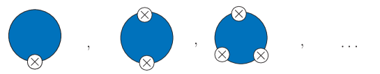
Figure 1: One-point, two-point, three-point, $\cdots$ vertex functions. The crosses can be vector or axial-vector currents and scalar or pseudo-scalar densities.

These vertex functions are glued into infinite geometrical series with couplings $g_{V}$ for vector or axial-vector sources and $g_{S}$ for scalar or pseudo-scalar sources, what can be seen as a very crude approximation to the two-particle reducible part. In this way one can construct full n-point Green’s functions in the presence of current quark masses –see for instance, how to get full two-point functions in Figure 2.

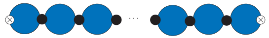
Figure 2: Infinite geometrical series which gives full two-point functions at large $N_{c}$. The black vertices that glue the vertex functions together are either $g_{V}$ for vector or axial-vector sources or $g_{S}$ for scalar and pseudo-scalar sources.

The basic vertex functions in Figure 1 have to be polynomials in momenta and quark masses to keep the large $N_{c}$ structure. As explained in [19], only the first nonet of hadronic states per channel, i.e., the pseudo-scalar pseudo-Goldstone bosons, the first vectors, the first axial-vectors and the first scalars can be easily generated within this framework. The coefficients of the vertex functions are free constants of order $N_{c}$, many of which can be fixed by imposing chiral Ward identities on the full Green’s functions. Chiral perturbation theory at order $p^{4}$ and the operator product expansion in QCD help to determine many more of these free coefficients in the vertex functions. A consequence of the formalism described here is that the vertex functions obey Ward identities with a constituent quark mass [19].

The full two-point Green’s functions obtained from the resummation in Figure 2 agree with the ones of large $N_{c}$ QCD when one limits the hadronic content to be just one hadronic state per channel –our model does not produce any less or more constraints than large $N_{c}$ QCD and all parameters can be fixed in terms of resonance masses [15] in agreement with other groups using large $N_{c}$ and one state per channel. Introducing two or more hadronic states per channel systematically is difficult as explained in [19]. We leave for future work the investigation into how to carry it out.

Most low-energy hadronic effective actions used for large $N_{c}$ phenomenology are in the approximation of keeping the resonances below some hadronic scale and always in the chiral limit. In many cases less than the four states included here are used.

The procedure described above of obtaining full Green’s functions can be done in the presence of current quark masses. In fact, in [15] two-point functions were calculated outside the chiral limit and all the new parameters that appear up to order $m_{q}^{2}$ can be determined except one; namely, the second derivative of the quark condensate with respect to quark masses. Some predictions of the model we are discussing involving coupling constants and masses of vectors and axial-vectors in the presence of masses are

$$f^{2}_{Vij}\,M^{2}_{Vij} = f^{2}_{Vkl}\,M^{2}_{Vkl}\,,$$

$$f^{2}_{Vij}\,M^{4}_{Vij}-f^{2}_{Vkl}\,M^{4}_{Vkl} = -\frac{1}{2}\langle\overline{q}q\rangle_{\chi}\,\left(m_{i}+m_{j}-m_{k}-m_{l}\right)\,$$

$$f^{2}_{Aij}\,M^{2}_{Aij}+f^{2}_{ij} = f^{2}_{Akl}\,M^{2}_{Akl}+f^{2}_{kl}\,,$$

$$f^{2}_{Aij}\,M^{4}_{Aij}-f^{2}_{Akl}\,M^{4}_{Akl} = \frac{1}{2}\langle\overline{q}q\rangle_{\chi}\,\left(m_{i}+m_{j}-m_{k}-m_{l}\right)\,,$$ (24)

where $i,j,k,l$ are indices for the up, down and strange quark flavors.

Three-point functions, as shown in Figure 3, were calculated in the chiral limit in [19]. We have now all the needed ones in the study of $\hat{B}_{K}$ also outside the chiral limit and they will be presented elsewhere [26].

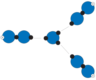
Figure 3: Infinite geometrical series which gives full three-point functions at large $N_{c}$. The crosses that glue the vertex functions are either $g_{V}$ for vector or axial-vector sources or $g_{S}$ for scalar and pseudo-scalar sources.

Some three-point functions have also been calculated in other large $N_{c}$ approaches and in the chiral limit [27, 28, 29, 30] –for instance, PVV, PVA, PPV and PSP three-point functions, where P stands for pseudo-scalar, V for vector, A for axial-vector and S for scalar sources. They agree fully with the ones we get in our model when restricted to just one hadronic state per channel.

Four-point functions are constructed analogously with the two-topologies dictated by large $N_{c}$, one with two three-point vertex functions and one with a four-point vertex function. The final four-point functions fulfill the correct chiral Ward identities –including current quark masses and we impose short-distance QCD constraints as well as the ChPT results at NLO to determine the free parameters allowed by the chiral Ward identities.

5 Chiral Limit Results

We now calculate $F[Q^{2}]$ of Eq. (17) in the chiral limit using the model of the previous section. After integrating over the four-dimensional Euclidean solid angle $\Omega_{Q}$ and doing the limit $q^{2}\to 0$ as in (17), we get

$$F^{\chi}[Q^{2}] = \delta_{1}Q^{2}+\delta_{2}+\frac{\alpha_{V}}{Q^{2}+M_{V}^{2}}+\frac{\alpha_{A}}{Q^{2}+M_{A}^{2}}+\frac{\alpha_{S}}{Q^{2}+M_{S}^{2}}+\frac{\beta_{V}}{\left(Q^{2}+M_{V}^{2}\right)^{2}}$$ (25)

$$+ \frac{\beta_{A}}{\left(Q^{2}+M_{A}^{2}\right)^{2}}+\frac{\gamma_{V}}{\left(Q^{2}+M_{V}^{2}\right)^{3}}+\frac{\gamma_{A}}{\left(Q^{2}+M_{A}^{2}\right)^{3}}\,.$$

We have used here the two-point vertex functions to second order in momenta, higher orders will make it impossible to satisfy the Weinberg sum rules. The three- and four-point vertex functions have been expanded to fourth order in the external momenta. The short-distance constraints used are the Weinberg sum rules and the fact that the vector form factor should vanish as $1/Q^{2}$ for large $Q^{2}$. As expected from the arguments in [19], we find clashes between short-distance constraints for three-point functions and those of the needed four-point function here. I.e., with just a finite number of hadronic states per channel not all short-distance constraints for n-point Green are compatible in general. Of course, one can always impose the latter which are compatible with the subset of the short-distance constraints corresponding to the momenta structure of the three-point functions entering in the four-point functions but not with all three-point functions short-distance constraints. That is what we have done for calculating $\hat{B}_{K}$.

The short-distance constraints on $F[Q^{2}]$ discussed in Sect. 3 and Ref. [17, 18] require $\delta_{1}=\delta_{2}=0$ in (25). Imposing these we obtain the expression for $F[Q^{2}]$ given in the appendix.

The explicit calculation reveals that diagrams with the exchange of vector and axial-vector states produce not only single poles but also double and triple poles. These also arise from diagrams with only one of these propagators due to the factor $1/q^{2}$ present in (17).

The function $F^{\chi}[Q^{2}]$ in (17) reproduces the large $N_{c}$-pole structure found in [17, 18] but including the first hadronic state in all the spin zero and one channels.

The relevant free parameters are the masses $M_{V}$, $M_{A}$ and $M_{S}$, the pion decay constant in the chiral limit, $F_{0}$, and three combinations of constants appearing in the three- and four-point vertex functions, $A_{1,2,3}^{\chi}$.

The low energy inputs we use are $F_{0}$ and the ${\cal O}(p^{4})$ couplings $L_{i}$ determined from the ChPT fits to data. We use two different fits, namely, fit 10 of [31] for $L_{1,2,3}$ and $L_{9,10}$ fit from [32], both with the full $p^{6}$ fits and the ones using only $p^{4}$ expressions. The input values for these two cases $p^{6}$ and $p^{4}$ are given together with some derived quantities in Table 1.

$p^{6}$ input $p^{4}$ input $F_{0}$ 87.7 MeV 81.1 MeV $10^{3}\,L_{1}$ 0.43 0.38 $10^{3}\,L_{2}$ 0.73 1.59 $10^{3}\,L_{3}$ $-$2.3 $-$2.91 $10^{3}\,L_{5}$ 0.97 1.46 $10^{3}\,L_{9}$ 5.93 6.9 $10^{3}\,L_{10}$ $-$4.4 $-$5.5 $M_{V}$ 805 MeV 690 MeV $M_{A}$ 1.16 GeV 895 MeV $M_{S}$ 1.41 GeV 1.06 GeV $A_{4}$ $-$12.7 $GeV^{-2}$ $-$23 $GeV^{-2}$

Table 1: The low energy inputs used together with some derived quantities for the two sets of input.

The values of the masses and the slope $A_{4}$ follow from the $L_{i}$ and $F_{0}$ used as input using the relations of [19] and (23). One could also use the physical masses and then use the $L_{i}$ only to get at the slope. The case with $p^{6}$ input is within 30% of the physical masses. For the scalars, which mass to use is still an open question, but with the mounting evidence that the first one are not present in large $N_{c}$, [33] and references therein, a mass of around 1.4 GeV seems fine.

We determine $A_{1}^{\chi}$ from the slope $A_{4}$ as given in (23) and the numerical values from Table 1.

$A_{2}^{\chi}$ and $A_{3}^{\chi}$ are obtained using the short distance constraints of (18), via

$$F[Q^{2}]_{SD}=\frac{D_{6}}{Q^{2}}+\frac{D_{8}}{Q^{4}}+{\cal O}\left(\frac{1}{Q^{6}}\right)\,.$$ (26)

We use the estimate $D_{8}/D_{6}\approx 0.13$ GeV^-2 of [18] but with rather large uncertainties. $D_{6}$ is calculated from (20) which contains the value of $\hat{B}_{K}$ inside it. One can choose here the large $N_{c}$ values or the values which come out of the analysis. We choose the latter ones using $\hat{B}_{K}=0.17,0.37$ for the $p^{6},p^{4}$ inputs, respectively. With $\alpha_{S}(m_{\tau})=0.35$ we obtain $D_{6}=0.0.028,0.052~{}$GeV² and $D_{8}=0.0036,0.0068~{}$GeV⁴. In the remainder we use the short-distance (26) with these values.

We have then used two different ways to match the model $F[Q^{2}]$ to short distance. The first one is to have the two coincide at the values of $Q^{2}=2$ and 3 GeV², these are labeled with “values” in the figures. The other is to have the model reproduce the values of $D_{6}$ and $D_{8}$ in its large $Q^{2}$ expansion, this case is labeled “order” in the figures.

In Fig. 4 we have plotted the short-distance curve and the model curves as well as the order $p^{4}$ ChPT approximation.

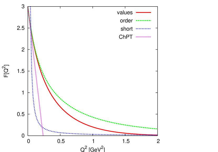
(a)

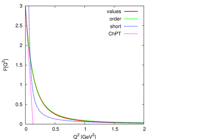
(b)

Figure 4: $F[Q^{2}]$ from ChPT, short distance and the large $N_{c}$ ladder resummation model interpolation. (a) with the $p^{6}$ fit values as input (b) with the $p^{4}$ fit values as input.

We now use (22) and integrate (17) up to the matching point $\mu$ and from that point on we use the OPE result including dimension eight corrections [18] of (26). This OPE contribution to $\hat{B}_{K}^{\chi}$ is negligible. In Figure 5, we plot this result as a function of $\mu^{2}$ Notice the nice plateau one gets between 1 and 2 GeV², with the exception of the case “order” with the $p^{6}$ input. From Fig.4a it can be seen that this because this case has an extremely slow approach to the short-distance.

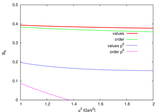
Figure 5: $\hat{B}_{K}^{\chi}$ plotted vs the upper limit of the integral in (17). See text for further explanation.

Varying the inputs within does not change the result more than those shown. We thus obtain

$$\hat{B}_{K}^{\chi}=0.38\pm 0.15\,$$ (27)

which is fully compatible with the one found previously also in the chiral limit in [14, 15, 17, 18].

6 Outside the Chiral Limit Results

The QCD results of the two energy regimes explained in Section 3 are known outside the chiral limit too.

The function $F[Q^{2}]$ is known for very large values of $Q^{2}$, which can be calculated using the OPE in QCD. In fact, the dimension six operator and Wilson coefficient are the same as the chiral limit ones. Differences will first start to appear at dimension 8 and we expect them to be small given the overall small estimate of the dimension 8 corrections.

At small values of $Q^{2}$ we can use ChPT. It is easy to get that $F[0]=0$ for the real case instead of $F^{\chi}[0]=3$ in the chiral limit. Notice that the value of $F^{\chi}[0]$ is a strong constraint on the value of $\hat{B}_{K}^{\chi}$. That $F[0]=0$ outside the chiral limit is a strong indication that corrections to the leading in $N_{c}$ value $B_{K}=3/4$ will be much smaller than in the chiral limit case.

The ChPT calculation in the real quark masses case of $F[Q^{2}]$ has been done to order $p^{4}$ [22] and $F[Q^{2}]$ remains small –below 0.15– up to energies around 0.2 GeV² and then goes negative.

Outside the chiral limit and to chiral order $p^{2}$, we get

$$F[Q^{2}]^{(2)} = -\frac{Q^{6}+2m_{K}^{2}Q^{4}+2m_{K}^{4}Q^{2}}{m_{K}^{2}(Q^{2}+m_{K}^{2})^{2}}+\frac{1}{4}\frac{Q^{2}+2m_{K}^{2}+2m_{\pi}^{2}}{m_{K}^{2}}\,I[Q^{2},m_{K}^{2},m_{\pi}^{2}]$$ (28)

$$+\frac{3}{4}\frac{Q^{2}+2m_{K}^{2}+2m_{\eta_{8}}^{2}}{m_{K}^{2}}\,I[Q^{2},m_{K}^{2},m_{\eta_{8}}^{2}]\,.$$

To chiral order $p^{4}$ and leading in $1/N_{c}$ we get

$$F[Q^{2}] = F[Q^{2}]^{(2)}-4\,(2L_{1}+5L_{2}+L_{3})\frac{3Q^{6}+6m_{K}^{2}Q^{4}+4m_{K}^{4}Q^{2}}{F_{\pi}^{2}(Q^{2}+m_{K}^{2})^{2}}$$ (29)

$$+8L_{5}\frac{Q^{6}+2m_{K}^{2}Q^{4}+2m_{K}^{4}Q^{2}}{F_{\pi}^{2}(Q^{2}+m_{K}^{2})^{2}}+16L_{8}\frac{m_{K}^{2}Q^{4}}{F_{\pi}^{2}(Q^{2}+m_{K}^{2})^{2}}+4L_{9}\frac{Q^{4}}{m_{K}^{2}F_{\pi}^{2}}$$

$$-2L_{5}\frac{Q^{2}m_{K}^{2}-m_{\pi}^{4}+m_{K}^{4}+4m_{\pi}^{2}m_{K}^{2}}{m_{K}^{2}F_{\pi}^{2}}I[Q^{2},m_{K}^{2},m_{\pi}^{2}]$$

$$-6L_{5}\frac{Q^{2}m_{K}^{2}-m_{\eta}^{4}+m_{K}^{4}+4m_{\eta}^{2}m_{K}^{2}}{m_{K}^{2}F_{\pi}^{2}}I[Q^{2},m_{K}^{2},m_{\eta_{8}}^{2}]$$

$$-L_{9}\frac{Q^{4}+(m_{K}^{2}-m_{\pi}^{2})^{2}+2Q^{2}(m_{K}^{2}+m_{\pi}^{2})}{m_{K}^{2}F_{\pi}^{2}}I[Q^{2},m_{K}^{2},m_{\pi}^{2}]$$

$$-3L_{9}\frac{Q^{4}+(m_{K}^{2}-m_{\eta_{8}}^{2})^{2}+2Q^{2}(m_{K}^{2}+m_{\eta_{8}}^{2})}{m_{K}^{2}F_{\pi}^{2}}I[Q^{2},m_{K}^{2},m_{\eta_{8}}^{2}]\,.$$

The angular integration results in the function

$$I[x,m_{1},m_{2}]\equiv\frac{x-m_{1}+m_{2}}{2m_{1}}\left[\sqrt{1+4m_{1}\,x/(x-m_{1}+m_{2})^{2}}-1\right]\,.$$ (30)

We have used the Gell-Mann-Okubo relation to simplify the $p^{4}$ contribution and dropped all terms that are subleading in $1/N_{c}$ as well as changed $F_{0}^{2}$ in the higher order to $F_{\pi}^{2}$.

In Fig. 6 we have shown $F[Q^{2}]$ at low $Q^{2}$ from the formulas above in ChPT for definiteness with the $p^{6}$ inputs of Table 1. It can be seen that the function starts at zero and the area under the curves, which gives the corrections is much smaller away from the chiral limit. The discontinuity in the curve is due to the fact that to the right the state with an intermediate pion can go on-shell.

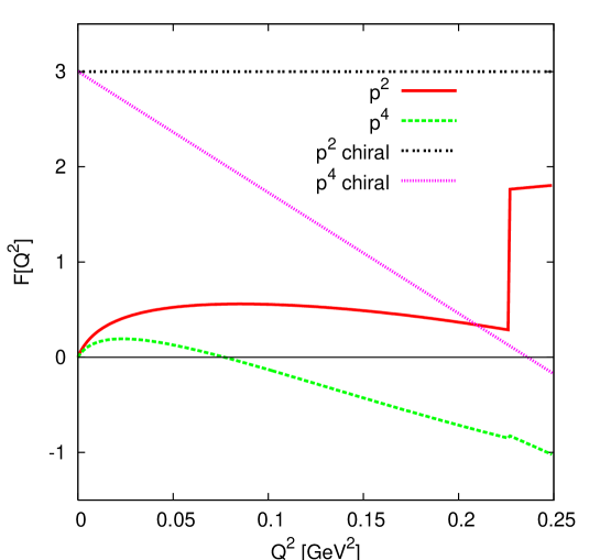
Figure 6: The ChPT calculation of $F[Q^{2}]$ in and away from the chiral limit.

One expects that higher ChPT order terms correct the behaviour of $F[Q^{2}]$ for $Q^{2}>$ 0.2 GeV² and $F[Q^{2}]$ will tend to the chiral limit curve in Figure 4. The question is at which energy does it happens. This can only be answered using a hadronic large $N_{c}$ approximation to QCD at present. So, though we have strong indications that the value $\hat{B}_{K}=3/4$ has small chiral corrections as shown before, we have to wait till we get the full four-point Green’s function in the real case (13) to confirm it. The number of new free parameters in our hadronic model including quark masses is rather high and we have at present not been able to determine all as we did in the chiral limit discussed earlier. We will eventually present the full result in the presence of current quark masses in [20].

7 Summary and Conclusions

In the past few years, lattice QCD has produced many calculations of $B_{K}$ using different fermion formulations –see [6, 7, 8] for references. Those include some chiral limit extrapolations –like for instance in [34] obtaining $\hat{B}_{K}^{\chi}=0.32\pm 0.22$ with quenched staggered quarks, in [35] obtaining $\hat{B}_{K}^{\chi}=0.34\pm 0.02$ with two dynamical domain wall quark flavours or in [36] obtaining $\hat{B}_{K}^{\chi}=0.39\pm 0.03$ with quenched domain wall quarks –which show a clear decreasing tendency with respect to the real case value, in agreement with the results found here and in [14, 15, 17, 18]. Promising preliminary unquenched results have also started to appear in the last two years [35, 37].

The QCD-Hadronic Duality result for $\hat{B}_{K}$[2, 3] is very close to the chiral limit result above because –as already mentioned in [3]– what was calculated there, is the order $p^{2}$ coefficient of the chiral expansion which actually is the chiral limit value of $\hat{B}_{K}$.

We have found values in this paper which are very compatible with the those chiral limit values and in agreement with those of [14, 15, 17, 18]. The improvement over our earlier work [14, 15] is the use of a more reliable model for the intermediate energy regime. What we have done beyond the work of [17, 18] is to include more resonances and a somewhat different input for the low-energy constants. In addition we have argued that away from the chiral limit the corrections to the LO large $N_{c}$ value 3/4 should be much smaller. A full result in the presence of current quark masses will be presented in [20].

Appendix A The Explicit Form of $F[Q^{2}]$

The function $F[Q^{2}]$ has in the chiral limit the form of Eq. (25). The short distance already imposes

$$\delta_{1}=\delta_{2}=0\,.$$ (31)

The remaining constants are

$$\alpha_{V} = -\frac{6M_{V}^{6}}{\left(M_{V}^{2}-M_{A}^{2}\right)^{2}}-\frac{3M_{V}^{4}}{M_{V}^{2}-M_{A}^{2}}-\frac{3}{4}M_{V}^{2}+\frac{15}{4}\frac{M_{V}^{4}}{M_{A}^{2}}+\frac{12M_{V}^{8}}{M_{A}^{2}}A_{3}^{\chi}+\frac{3}{128}M_{V}^{6}N_{\pi}$$

$$\alpha_{A} = \frac{6M_{V}^{6}}{\left(M_{V}^{2}-M_{A}^{2}\right)^{2}}+\frac{3M_{V}^{4}}{M_{V}^{2}-M_{A}^{2}}-\frac{3M_{V}^{4}M_{S}^{2}}{\left(M_{A}^{2}-M_{S}^{2}\right)^{2}}+\frac{15}{2}\frac{M_{A}^{4}}{M_{V}^{2}}-\frac{33}{4}M_{V}^{2}+\frac{9}{4}\frac{M_{V}^{4}}{M_{A}^{2}}-\frac{9}{2}M_{A}^{2}$$

$$+\frac{12M_{V}^{6}}{M_{A}^{2}}A_{1}^{\chi}-\frac{12M_{S}^{6}}{\left(M_{A}^{2}-M_{S}^{2}\right)^{2}}A_{2}^{\chi}+12M_{S}^{2}A_{2}^{\chi}-12M_{V}^{6}A_{3}^{\chi}+\frac{1}{384}\frac{M_{A}^{8}}{M_{V}^{2}}N_{\pi}$$

$$\alpha_{S} = \frac{3M_{V}^{4}M_{S}^{2}+12M_{S}^{6}A_{2}^{\chi}}{\left(M_{A}^{2}-M_{S}^{2}\right)^{2}}$$

$$\beta_{V} = -\frac{3M_{V}^{6}M_{A}^{2}}{\left(M_{V}^{2}-M_{A}^{2}\right)^{2}}+\frac{9}{4}M_{V}^{4}-\frac{3M_{V}^{6}}{M_{A}^{2}}-\frac{6M_{V}^{10}}{M_{A}^{2}}A_{3}^{\chi}-\frac{3}{64}M_{V}^{8}N_{\pi}$$

$$\beta_{A} = \frac{3M_{V}^{8}}{\left(M_{V}^{2}-M_{A}^{2}\right)^{2}}-\frac{9M_{V}^{6}}{M_{V}^{2}-M_{A}^{2}}-\frac{3M_{V}^{4}M_{S}^{2}}{M_{A}^{2}-M_{S}^{2}}-\frac{15}{2}\frac{M_{A}^{6}}{M_{V}^{2}}+\frac{3}{2}M_{V}^{2}M_{A}^{2}+\frac{3}{4}M_{V}^{4}+3M_{A}^{4}$$

$$-12M_{V}^{6}A_{1}^{\chi}-\frac{12M_{A}^{4}M_{S}^{2}}{M_{A}^{2}-M_{S}^{2}}A_{2}^{\chi}+6M_{V}^{6}M_{A}^{2}A_{3}^{\chi}-\frac{1}{192}\frac{M_{A}^{10}}{M_{V}^{2}}N_{\pi}$$

$$\gamma_{V} = -\frac{3M_{V}^{6}M_{A}^{2}}{M_{V}^{2}-M_{A}^{2}}+\frac{3}{128}M_{V}^{10}N_{\pi}$$

$$\gamma_{A} = -\frac{3M_{V}^{2}M_{A}^{6}}{M_{V}^{2}-M_{A}^{2}}+\frac{1}{384}\frac{M_{A}^{12}}{M_{V}^{2}}N_{\pi}$$ (32)

The parts proportional to $N_{\pi}$ defined by

$$N_{\pi}=\frac{N_{c}^{2}}{F_{0}^{4}\pi^{4}}\left(1-\frac{M_{V}^{2}}{M_{A}^{2}}\right)\,,$$ (33)

come from the diagrams with anomalous three-point vertex functions.

References

- [1] A. J. Buras, “Weak Hamiltonian, CP violation and rare decays,” Les Houches lectures 1998, hep-ph/9806471; G. Buchalla, A.J. Buras and M.E. Lautenbacher, Rev. Mod. Phys. 68 (1996) 1125.
- [2] A. Pich and E. de Rafael, Phys. Lett. B 158 (1985) 477.
- [3] J. Prades, C.A. Domínguez, J.A. Peñarrocha, A. Pich and E. de Rafael, Z. Phys. C 51 (1991) 287.
- [4] K.G. Chetyrkin et al. Phys. Lett. B 174 (1986) 104; R. Decker, Nucl. Phys. B 277 (1986) 660; N. Bilić, B. Guberina and C.A. Domínguez, Z. Phys. C 39 (1988) 351; R. Decker, Nucl. Phys. B (Proc. Suppl.) 7A (1989) 180.
- [5] “The CKM Matrix and the Unitarity Triangle”, M. Battaglia, A.J. Buras, P. Gambino, and A. Stocchi (eds), CERN (2003), hep-ph/0304132. J. Charles et al. [CKMfitter Group], Eur. Phys. J. C 41 (2005) 1; M. Bona et al. [UTfit Collaboration], J. High Energy Phys. 07 (2005) 028.
- [6] M. Wingate, Nucl. Phys. B (Proc. Suppl.) 140 (2005) 68.
- [7] S. Hashimoto in Proc. of ICHEP 2004, Vol I, p. 77, H. Chen et al, (eds), World Scientific (2005), hep-ph/0411126.
- [8] C. Dawson, PoS LAT2005 (2005) 007.
- [9] G. ’t Hooft, Nucl. Phys. B 72 (1974) 461; bid. B 75 (1974) 461.
- [10] E. Witten, Nucl. Phys. B 160 (1979) 57.
- [11] W.A. Bardeen, A.J. Buras and J.-M. Gérard, Phys. Lett. B 180 (1986) 133, Nucl. Phys. B 293 (1987) 787; Phys. Lett. B 192 (1987) 138; Phys. Lett. B 211 (1988) 343; A.J. Buras and J.-M. Gérard, Nucl. Phys. B (Proc. Suppl.) 7A (1989) 375; J.-M. Gérard, Acta Phys. Polon. B 21 (1990) 257; A.J. Buras in “CP Violation”, p. 575, C. Jarslkog (ed), World Scientific (1989).
- [12] W.A. Bardeen, Nucl. Phys. B (Proc. Suppl.) 7A (1989) 149.
- [13] W.A. Bardeen in “Kaon Physics”, p. 171, J.L. Rosner and B.D. Winstein (eds), Univ. Chicago Press (2001).
- [14] J. Bijnens and J. Prades, Phys. Lett. B 342 (1995) 331; Nucl. Phys. B 444 (1995) 523.
- [15] J. Bijnens and J. Prades, J. High Energy Phys. 01 (2000) 002.
- [16] J. Bijnens, C. Bruno and E. de Rafael, Nucl. Phys. B 390 (1993) 501; J. Prades, Z. Phys. C 63 (1994) 491 [Erratum Eur. J. Phys. C 11 (1999) 571]; J. Bijnens, E. de Rafael and H.q. Zheng, Z. Phys. C 62 (1994) 437; J. Bijnens and J. Prades, Phys. Lett. B 320 (1994) 130; Z. Phys. C 64 (1994) 475; Nucl. Phys. B (Proc. Suppl.) 39BC (1995) 245; J. Bijnens, Phys. Rept. 265 (1996) 369.
- [17] S. Peris and E. de Rafael, Phys. Lett. B 490 (2000) 213 [Erratum, hep-ph/0006146].
- [18] O. Catà and S. Peris, J. High Energy Phys. 03 (2003) 060.
- [19] J. Bijnens, E. Gámiz, E. Lipartia and J. Prades, J. High Energy Phys. 04 (2003) 055.
- [20] J. Bijnens, E. Gámiz and J. Prades, in preparation.
- [21] J. Bijnens, E. Gámiz and J. Prades, J. High Energy Phys. 10 (2001) 009.
- [22] J. Bijnens and J. Prades, presented at the second EURIDICE collaboration meeting, 6-8 february 2003, Orsay.
- [23] J. Prades, J. Bijnens and E. Gámiz, “Trento 2004, Large QCD”, p. 179-190, J.L. Goity et al (eds.), World Scientific (2005), hep-ph/0501177.
- [24] A.J. Buras, M. Jamin and P.H. Weisz, Nucl. Phys. B 347 (1990) 491; S. Herrlich and U. Nierste, Nucl. Phys. B 419 (1994) 292; Phys. Rev. D 52 (1995) 6505; Nucl. Phys. B 476 (1996) 27; M. Ciuchini, E. Franco, V. Lubicz, G. Martinelli, I. Scimemi and L. Silvestrini, Nucl. Phys. B 523 (1998) 501.
- [25] V. Cirigliano, J.F. Donoghue and E. Golowich, J. High Energy Phys. 10 (2000) 048.
- [26] J. Bijnens, E. Gámiz and J. Prades, in preparation.
- [27] B. Moussallam and J. Stern, hep-ph/9404353; B. Moussallam, Phys. Rev. D 51 (1995) 4939; Nucl. Phys. B 504 (1997) 381.
- [28] M. Knecht and A. Nyffeler, Eur. Phys. J. C 21 (2001) 659.
- [29] V. Cirigliano, G. Ecker, M. Eidemüller, A. Pich and J. Portolés, Phys. Lett. B 596 (2004) 96.
- [30] P.D. Ruiz-Femenía, A. Pich and J. Portolés, J. High Energy Phys. 07 (2003) 003; Nucl. Phys. B (Proc. Suppl.) 133 (2004) 215.
- [31] G. Amorós, J. Bijnens and P. Talavera, Nucl. Phys. B 602 (2001) 87.
- [32] J. Bijnens and P. Talavera, J. High Energy Phys. 03 (2002) 046; Nucl. Phys. B 489 (1997) 387.
- [33] V. Cirigliano, G. Ecker, H. Neufeld and A. Pich, J. High Energy Phys. 06 (2003) 012.
- [34] W. Lee et al., Phys. Rev. D 71 (2005) 094501.
- [35] Y. Aoki et al., Phys. Rev. D 72 (2005) 114505.
- [36] Y. Aoki et al., hep-lat/0508011.
- [37] E. Gámiz, S. Collins, C. T. H. Davies, J. Shigemitsu and M. Wingate [HPQCD Collaboration], PoS LAT2005 (2005) 47; T. Bae, J. Kim and W. Lee, ibid 335; ibid 338; S. Cohen, ibid 346; F. Mescia, V. Giménez, V. Lubicz, G. Martinelli, S. Simula and C. Tarantino, ibid 365; J. M. Flynn, F. Mescia and A. S. B. Tariq [UKQCD Collaboration], J. High Energy Phys. 11 (2004) 049.