See-saw Fermion Masses in an SO(10) GUT

Abstract

In this work we study an SO(10) GUT model with minimum Higgs representations belonging only to the 210 and 16 dimensional representations of SO(10). We add a singlet fermion $S$ in addition to the usual 16 dimensional representation containing quarks and leptons. There are no Higgs bi-doublets and so charged fermion masses come from one-loop corrections. Consequently all the fermion masses, Dirac and Majorana, are of the see-saw type. We minimize the Higgs potential and show how the left-right symmetry is broken in our model where it is assumed that a $D$-parity odd Higgs field gets a vacuum expectation value at the grand unification scale. From the renormalization group equations we infer that in our model unification happens at $10^{15}$ GeV and left-right symmetry can be extended up to some values just above $10^{11}$ GeV. The Yukawa sector of our model is completely different from most of the standard grand unified theories and we explicitly show how the Yukawa sector will look like in the different phases and briefly comment on the running of the top quark mass. We end with a brief analysis of lepton number asymmetry generated from the interactions in our model.

1 Introduction

The SO(10) grand unified theory has several interesting features [1, 2, 3, 4, 5]. It can accommodate left-right symmetry as one of the intermediate symmetry and hence provides an explanation of parity violation [6]. $(B-L)$ is a generator of the group SO(10) and hence lepton number violation takes place spontaneously. This explains the origin of lepton number violation and neutrino Majorana mass naturally. The smallness of neutrino masses is assured by the see-saw mechanism, so that by keeping the scale of $(B-L)$ violation high the smallness of the neutrino mass is guaranteed. Quarks and leptons are treated equally in SO(10) GUT. Gauge coupling unification is consistent with all low energy results.

On the one hand there are many attractive features of the SO(10) GUT, on the other the predictability becomes low. Depending on the symmetry breaking pattern and Higgs scalar contents, the model can have widely differing predictions. Attempts have been made to construct a minimal model. In one approach the minimal model is constructed with minimum numbers of parameters, while in the other approach minimum numbers of Higgs scalars are included in the model. There are also models without any intention of minimality or simplicity, where the main aim is to explain all experiments and have maximum predictability.

In the present article we shall study an SO(10) GUT, which has the minimum dimensions of the Higgs scalars. In any SO(10) GUT the minimal number of Higgs scalar includes an ${\rm SU(2)}_{L}$ symmetry breaking Higgs scalar, which can give masses to the fermions and some scalars that can break the $(B-L)$ symmetry along with the ${\rm SU(2)}_{R}$ symmetry and can give Majorana masses to the neutrinos. In addition, there is one Higgs scalar which breaks the group SO(10) GUT. One conventional model includes a Higgs bi-doublet (a 10-plet of SO(10) Higgs scalar, which is doublet under both the ${\rm SU(2)}_{L}$ and ${\rm SU(2)}_{R}$ groups) and both ${\rm SU(2)}_{L}$ and ${\rm SU(2)}_{R}$ Higgs triplets. In such models with triplet Higgs scalars neutrinos acquire masses at the tree level. The SO(10) representation that contains this Higgs scalar is of 126 dimensions. In another version of the model, one breaks the left-right symmetry and the $(B-L)$ symmetry by doublets of ${\rm SU(2)}_{L}$ and ${\rm SU(2)}_{R}$ groups. This Higgs field belongs to a 16-plet representation of SO(10). For symmetry breaking and giving fermion masses another 10-plet Higgs scalar is introduced, which contains the bi-doublet Higgs and hence gives tree level masses to the fermions and the neutrinos acquire only Dirac masses of the order of other fermion masses. There is no Majorana mass term for the neutrinos and hence see-saw mechanism is not possible. However, there exist effective higher-dimensional operators, which can give correct Majorana masses to both the left-handed and right-handed neutrinos.

Recently it has been pointed out that it is possible to consider an SO(10) GUT, which does not have any Higgs bi-doublet scalar belonging to a 10-plet of SO(10) [7]. The Higgs scalar that breaks left-right symmetry and the $(B-L)$ symmetry belongs to a 16-plet of Higgs scalar. Since tree level fermion masses are not allowed without the bi-doublet scalar, all fermion masses come from higher-dimensional operators in the see-saw form. In supersymmetric theories the non-renormalizablity theorem does not allow radiative generation of such higher dimensional operators. We shall then restrict ourselves to only non-supersymmetric SO(10) GUT. The source of see-saw suppression for the fermion number violating Majorana mass terms are different from the source of see-saw suppression for the fermion number conserving Dirac mass terms, which maintain the large hierarchy between the charged fermion masses and the neutrino masses. In this article we shall study some aspects of this model in detail.

In the next section we shall discuss the model. In sec. 3 we shall present details of the scalar potential minimization and the allowed symmetry breaking pattern and in sec. 4 the generation of fermion masses is discussed. We shall then study the renormalization group equation for this model with the specific choice of the Higgs scalars. In sec. 5 we shall study the gauge coupling unification and in sec. 6 the Yukawa coupling evolution for the different fermions. Since all fermion masses have the same see-saw origin, the perturbative unification becomes an important question in these models. Some of the Yukawa couplings could become large, although the effective fermion masses still remains small. In sec. 7 leptogenesis in our model is discussed and in the last section we summarize our results.

2 The Model

The starting point for any SO(10) GUT is the choice of the symmetry breaking pattern. There exists many chains of symmetry breaking pattern, which are all consistent with our present knowledge. So the particular choice of a symmetry breaking pattern defines a specific model. We shall consider a symmetry breaking pattern, which requires a minimum number of Higgs scalars, given by:

$${\rm SO(10)} {\stackrel{{\scriptstyle\Phi_{D}}}{{\longrightarrow}}} {\rm SU(4)}_{C}\times{\rm SU(2)}_{L}\times{\rm SU(2)}_{R}\quad[{\rm G}_{422}]$$ (1)

$${\stackrel{{\scriptstyle\Phi_{4}}}{{\longrightarrow}}} {\rm SU(3)}_{C}\times{\rm SU(2)}_{L}\times{\rm SU(2)}_{R}\times{\rm U(1)}_{B-L}\quad[{\rm G}_{3221}]$$

$${\stackrel{{\scriptstyle\chi_{R}}}{{\longrightarrow}}} {\rm SU(3)}_{C}\times{\rm SU(2)}_{L}\times{\rm U(1)}_{Y}\quad[{\rm G}_{321}]$$

$${\stackrel{{\scriptstyle\chi_{L}}}{{\longrightarrow}}} {\rm SU(3)}_{C}\times{\rm U(1)}_{\rm em}\,,$$

where the Higgs fields responsible for the symmetry breakings, $\Phi_{D}$, $\Phi_{4}$, $\chi_{R}$ and $\chi_{L}$ are explicitly shown in the above equation. Both $\Phi_{D}$ and $\Phi_{4}$ are contained in $\Phi$, which transforms as the 210 dimensional representation of SO(10). The 210-plet decomposes under the Pati-Salam subgroup ${\rm G}_{422}$ of SO(10) as,

$$\Phi\equiv{\bf 210} = (\bf{1,1,1})+(\bf{6,2,2})+(\bf{15,3,1})+(\bf{15,1,3})$$ (2)

$$+\,(\bf{15,1,1})+(\bf{10,2,2})+(\overline{\bf 10},\bf{2,2})\,.$$

In the above decomposition $\Phi_{D}$ corresponds to $({\bf 1,1,1})$ and $\Phi_{4}$ corresponds to (15,1,1).

The Higgs fields $\chi_{L}$ and $\chi^{*}_{R}$ belong to the 16 dimensional spinor representation $\Gamma$ of SO(10) and the other fields $\chi_{R}$ and $\chi^{*}_{L}$ belong to the conjugate representation $\overline{\bf 16}$, called $\Gamma^{\dagger}$, of SO(10). The group transformation properties of the $\chi$ fields under ${\rm G}_{3221}$ and ${\rm G}_{422}$ are as follows:

$$\begin{array}[]{ccccc}\chi_{L}&\equiv&({\bf 1,2,1},-1)\subset({\bf 4,2,1})\subset{\bf 16}&\equiv&\Gamma\,,\\ \chi^{*}_{R}&\equiv&({\bf 1,1,2},1)\subset({\overline{\bf 4}},{\bf 1,2})\subset{\bf 16}&\equiv&\Gamma\,,\\ \chi_{R}&\equiv&({\bf 1,1,2},-1)\subset({\bf 4,1,2})\subset{\overline{\bf 16}}&\equiv&{\Gamma^{\dagger}}\,,\\ \chi^{*}_{L}&\equiv&({\bf 1,2,1},1)\subset({\overline{\bf 4}},{\bf 2,1})\subset{\overline{\bf 16}}&\equiv&{\Gamma^{\dagger}}\,.\end{array}$$ (7)

In the above equations $({\bf x,y,z},w)$, and $({\bf x,y,z})$ denote the group transformation properties of the Higgs fields under ${\rm G}_{3221}$ and ${\rm G}_{422}$.

At this stage we shall digress to discuss one important feature of the left-right symmetric models, namely the question of parity ${\cal P}$. The discrete $Z_{2}$ symmetry, that interchanges the two SU(2) subgroups of the Lorentz group O(3,1), is called the parity. This parity can be identified as the discrete $Z_{2}$ symmetry operator that interchanges the groups ${\rm SU(2)}_{L}$ and ${\rm SU(2)}_{R}$ of the left-right symmetric model, which implies that under parity $W_{L}\stackrel{{\scriptstyle\cal P}}{{\longleftrightarrow}}W_{R}$. This definition extends to scalars also. That is, an ${\rm SU(2)}_{L}$ doublet scalar field $\chi_{L}$ will transform to an ${\rm SU(2)}_{R}$ doublet scalar field $\chi_{R}$ under the operation of parity $\chi_{L}\stackrel{{\scriptstyle\cal P}}{{\longleftrightarrow}}\chi_{R}$. In the conventional left-right symmetric models, the parity is spontaneously broken along with the group ${\rm SU(2)}_{R}$. In other words, when the left-right symmetric group ${\rm SU(2)}_{L}\times{\rm SU(2)}_{R}$ is spontaneously broken, parity is also spontaneously broken.

There is another possibility of breaking parity spontaneously without breaking the left-right symmetric group. Since the scalar fields transform trivially under the Lorentz group, the VEV of a parity odd field can break parity spontaneously without breaking the left-right symmetry. Unlike the conventional case, now the parity acting on the fermions and vector bosons is not spontaneously broken. To distinguish these two cases, this second type of parity is called a $D$-parity. Thus when $D$-parity is broken, the left-handed and right-handed scalars can have different mass and VEV and hence the gauge coupling constants of ${\rm SU(2)}_{L}$ and ${\rm SU(2)}_{R}$ can also be different. In the present model $D$-parity plays a very crucial role, both for symmetry breaking as well as for fermion masses. It also plays some role in gauge coupling unification.

The ${\bf 210}$ representation of SO(10) is a totally antisymmetric tensor of rank four $\Phi_{abcd}$ and the singlet $\Phi_{D}$ is the component $\Phi_{6789}$ in the notation, in which, $a,b,c,d=0,1,..,5$ are ${\rm SO(6)}$ indices and $a,b,c,d=6,7,8,9$ are ${\rm SO(4)}$ indices. Thus under $D$-parity $\Phi_{D}$ is odd ($\Phi_{D}\to-\Phi_{D}$) and consequently when it gets its vacuum expectation value (VEV) at the GUT scale, $M_{U}$, it breaks the left-right parity of the theory. Due to this spontaneous breaking of the left-right parity at the $M_{U}$ scale we will have $\langle\chi_{L}\rangle\neq\langle\chi_{R}\rangle$ at a lower energy scale. This $D$-parity odd field is also required to give masses to the light neutrinos.

Next we write down the fermions in our model and their group transformation properties. The left-handed quarks, leptons, anti-quarks and anti-leptons belong to a 16-plet representation of SO(10), which transform under ${\rm G}_{422}$ as:

$$\psi_{i\,L}\equiv{\bf 16}=(\bf{4,2,1})+({\overline{\bf 4}},\bf{1,2})\,,$$ (8)

$i=1,2,3$ is the generation index. The right-handed fermions and anti-fermions belong to the conjugate representation,

$$\psi_{i\,R}\equiv{\overline{\bf 16}}=({\overline{\bf 4}},\bf{2,1})+(\bf{4,1,2})\,.$$ (9)

In addition to the above mentioned conventional particles our model consists of an extra SO(10) gauge singlet fermion per generation:

$$S_{iL}\equiv{\bf 1}=({\bf 1,1,1})\,,$$ (10)

$i=1,2,3$.

Under ${\rm G}_{3221}$ the states $(\bf{4,2,1})$ and $({\overline{\bf 4}},\bf{1,2})$ transform as:

$$(\bf{4,2,1}) = ({\bf 3,2,1},\frac{1}{3})+({\bf 1,2,1},-1)\,,$$ (11)

$$({\overline{\bf 4}},\bf{1,2}) = ({\overline{\bf 3}},{\bf 1,2},-\frac{1}{3})+({\bf 1,1,2},1)\,,$$ (12)

and as a result the fermions can be labelled as:

$$q_{L} = \left(\begin{array}[]{c}u\\ d\end{array}\right)_{L}\equiv({\bf 3,2,1},\frac{1}{3})\,,$$ (15)

$$\ell_{L} = \left(\begin{array}[]{c}\nu\\ e\end{array}\right)_{L}\equiv({\bf 1,2,1},-1)\,,$$ (18)

and

$$q^{\,\,\,\,c}_{R}=q^{c}_{\,\,L} = \left(\begin{array}[]{c}d^{\,c}\\ u^{c}\end{array}\right)_{L}\equiv({\overline{\bf 3}},{\bf 1,2},-\frac{1}{3})\,,$$ (21)

$$\ell^{\,\,\,\,c}_{R}=\ell^{c}_{\,\,L} = \left(\begin{array}[]{c}e^{c}\\ \nu^{c}\end{array}\right)_{L}\equiv({\bf 1,1,2},1)\,.$$ (24)

The generators of the left-right symmetry group ${\rm G}_{3221}$ are related to the electric charge of the particles by,

$$Q=T_{3L}+T_{3R}+\frac{(B-L)}{2}=T_{3L}+\frac{Y}{2}\,,$$ (25)

where

$$Y=T_{3R}+\frac{(B-L)}{2}\,.$$ (26)

In the conventional left-right symmetric models there is one bi-doublet Higgs scalar $\phi\equiv({\bf 1,2,2,}0)$, which gives masses to quarks and charged leptons and a Dirac mass to the neutrinos through its couplings of the form $\overline{\psi}_{L}\psi_{R}\phi$. In addition, there are triplet Higgs scalars $\Delta_{L}\equiv({\bf 1,3,1},-2)$ and $\Delta_{R}\equiv({\bf 1,1,3,}-2)$, which can give Majorana masses to the left-handed and right-handed neutrinos through the couplings $\psi_{L,R}\psi_{L,R}\Delta_{L,R}$. In our present model all these Higgs scalars $\phi$, $\Delta_{L}$ and $\Delta_{R}$ are absent and hence there are no tree level fermion masses for the quarks and the leptons. After discussing the structure of the Higgs vacuum expectation values in this model, we shall come back to the question of fermion masses.

3 Minimization of the scalar potential and left-right symmetry breaking

In the conventional left-right symmetric models, the combinations of the Higgs fields, $\phi$, $\Delta_{L}$ and $\Delta_{R}$ ensures that for certain choices of parameters, $\Delta_{R}$ can acquire a very large VEV compared to other fields breaking left-right symmetry at a large scale. It is clear that in the absence of the field $\phi$, both the fields $\Delta_{L,R}$ would acquire equal VEVs. It has also been shown that in the absence of the field $\phi$ in a left-right symmetric model with only the doublet Higgs scalars $\chi_{L}$ and $\chi_{R}$, the minimization of the potential would result in equal VEVs for both $\chi_{L}$ and $\chi_{R}$, which would lead to inconsistency and parity will be conserved at low energy. This problem could be solved if parity is broken in these theories either explicitly or spontaneously.

In the present model this problem does not occur. It was mentioned in the original version of the model that the $D$-parity odd singlet field $\Phi_{D}\equiv{\bf(1,1,1)}$ under G₄₂₂ contained in the ${\bf 210}$ representation would allow $\langle\chi_{R}\rangle\gg\langle\chi_{L}\rangle$ and break left-right symmetry at some high scale. In this section we shall minimize the scalar potential and discuss the various possible solutions, which allows left-right symmetry breaking at some high scale.

Let us consider the Higgs potential [7]:

$${\cal L}_{s} = m^{2}_{\Phi}\Phi^{2}+a\Phi^{3}+\frac{\lambda_{\Phi}}{4!}\Phi^{4}+m^{2}_{\Gamma}(\Gamma^{\dagger}\Gamma)+\frac{\lambda_{\Gamma}}{4}(\Gamma^{\dagger}\Gamma)^{2}$$ (27)

$$+\,\frac{\lambda^{\prime}_{\Gamma}}{4}[\Gamma^{4}+(\Gamma^{\dagger})^{4}]+M_{D}\Phi(\Gamma^{\dagger}\Gamma)+\lambda_{\Phi\Gamma}\Phi^{2}(\Gamma^{\dagger}\Gamma)\,.$$

The coupling $\Phi(\Gamma^{\dagger}\Gamma)$ is the most important term that is required for the left-right breaking to take place at a higher scale compared to standard model symmetry breaking. $D$-parity is broken when $\Phi_{D}$ acquires a non-vanishing VEV, $\langle\Phi_{D}\rangle=\eta$, at the $M_{U}$ scale, since $\Phi_{D}$ is odd under $D$-parity. $\Phi_{4}$ will get a non-vanishing VEV at the $M_{X}$ scale. There will be many terms in Eq. (27) including $\langle\Phi_{4}\rangle$, but as we are analyzing the structure of Eq. (27) in the ${\rm G}_{3221}$ phase and mainly interested on the VEVs of the $\chi$ fields, we do not explicitly write down the terms including $\langle\Phi_{4}\rangle$. $\langle\Phi_{4}\rangle$ has no important contribution in the expressions of the VEVs of the $\chi$ fields.

We now discuss the masses of the components of $\Gamma$ and the VEVs. The scalar potential responsible for the masses of the fields $\chi_{L}$ and $\chi_{R}$ is given by,

$$V = m_{\Gamma}^{2}(|\chi_{R}|^{2}+|\chi_{L}|^{2})+M_{D}~{}\eta(|\chi_{R}|^{2}-|\chi_{L}|^{2})$$ (28)

$$+\,\lambda_{\Phi\Gamma}~{}\eta^{2}(|\chi_{R}|^{2}+|\chi_{L}|^{2})\,.$$

The masses of these fields are then given by,

$$\mu_{L}^{2} = m_{\Gamma}^{2}-M_{D}~{}\eta+\lambda_{\Phi\Gamma}~{}\eta^{2}\,,$$

$$\mu_{R}^{2} = m_{\Gamma}^{2}+M_{D}~{}\eta+\lambda_{\Phi\Gamma}~{}\eta^{2}\,.$$ (29)

If $D$-parity is conserved, $\eta=0$ and the masses of both $\chi_{L}$ and $\chi_{R}$ become equal. Since the VEV of $\Phi_{D}$ breaks $D$-parity, it will be possible to fine tune parameters to obtain the mass of $\chi_{L}$ to be orders of magnitude smaller than the mass of $\chi_{R}$. From phenomenological consideration we also require

$$\langle\chi_{L}\rangle = v_{L}\sim\mu_{L}\sim 100~{}{\rm GeV}\,,$$

$$\langle\chi_{R}\rangle = v_{R}\sim\mu_{R}\sim M_{U}\gg v_{L}\,.$$ (30)

We shall next check if this widely different VEVs for $\chi_{L}$ and $\chi_{R}$ is possible. $v_{L}$ breaks the electroweak symmetry, while $v_{R}$ breaks the left-right symmetry at a very high scale, close to the GUT scale.

We denote the VEVs of the fields $\chi_{L}$ and $\chi_{R}$ as:

$$\langle\chi_{L}\rangle=\left(\begin{array}[]{c}v_{L}\\ 0\end{array}\right),\,\,\langle\chi^{*}_{R}\rangle=\left(\begin{array}[]{c}0\\ v^{*}_{R}\end{array}\right),\,\,\langle\chi_{R}\rangle=\left(\begin{array}[]{c}v_{R}\\ 0\end{array}\right),\,\,\langle\chi^{*}_{L}\rangle=\left(\begin{array}[]{c}0\\ v^{*}_{L}\end{array}\right).$$ (39)

Instead of minimizing the potential, we shall first write down the potential in terms of the VEVs of the fields and then find the conditions satisfied by the VEVs. With the above VEVs we can write the Higgs potential in the ${\rm G}_{3221}$ phase as:

$$V = -\,m^{2}_{\Phi}(\eta^{2}+\cdot\cdot\cdot)-a\,(\eta^{3}+\cdot\cdot\cdot)-\frac{\lambda_{\Phi}}{4!}(\eta^{4}+\cdot\cdot\cdot)$$ (40)

$$+\,[m^{2}_{\Gamma}+\lambda_{\Phi\Gamma}(\eta^{2}+\cdot\cdot\cdot)](v^{*}_{R}v_{R}+v^{*}_{L}v_{L})-\frac{\lambda_{\Gamma}}{4}(v^{*}_{R}v_{R}+v^{*}_{L}v_{L})^{2}$$

$$-\,\frac{\lambda^{\prime}_{\Gamma}}{4}(v^{4}_{L}+v^{4}_{R}+v^{*\,4}_{L}+v^{*\,4}_{R})+M_{D}\eta(v^{*}_{R}v_{R}-v^{*}_{L}v_{L})\,.$$

The $\cdot\cdot\cdot$ symbols in the above equation stands for terms containing $\langle\Phi_{4}\rangle$.

Setting $v_{R}=v^{*}_{R}$ and $v_{L}=v^{*}_{L}$, which amounts to saying that there is no CP violation and all VEVs are considered to be real, the extremum conditions of $V$ comes out to be:

$$\frac{\partial V}{\partial v_{L}} = 2v_{L}\left[m^{2}_{\Gamma}+(\lambda_{\Phi\Gamma}\eta^{2}+\cdot\cdot\cdot)-\frac{\lambda_{\Gamma}}{2}(v^{2}_{L}+v^{2}_{R})-\lambda^{\prime}_{\Gamma}v^{2}_{L}-M_{D}\eta\right]=0\,,$$

$$\frac{\partial V}{\partial v_{R}} = 2v_{R}\left[m^{2}_{\Gamma}+(\lambda_{\Phi\Gamma}\eta^{2}+\cdot\cdot\cdot)-\frac{\lambda_{\Gamma}}{2}(v^{2}_{L}+v^{2}_{R})-\lambda^{\prime}_{\Gamma}v^{2}_{R}+M_{D}\eta\right]=0\,.$$

The above equations imply,

$$v_{L}\left(\frac{\partial V}{\partial v_{R}}\right)-v_{R}\left(\frac{\partial V}{\partial v_{L}}\right)=2v_{L}v_{R}[\lambda^{\prime}_{\Gamma}(v^{2}_{L}-v^{2}_{R})+2M_{D}\eta]=0\,.$$ (43)

Neglecting the trivial solution $v_{L}=v_{R}=0$, the other interesting relation between $v_{L}$ and $v_{R}$ that comes out from the above equation is,

$$v^{2}_{R}-v^{2}_{L}=\frac{2M_{D}\eta}{\lambda^{\prime}_{\Gamma}}\,.$$ (44)

Two things can be noted from the above equation. First as it was stated previously, in understanding the relation between $v_{L}$ and $v_{R}$ we do not require the VEV of $\Phi_{4}$. Secondly if $\eta$ has some value comparable to $M_{U}$ and $\lambda^{\prime}_{\Gamma}$ is not too high, then it is apparent from Eq. (44) that $v_{R}\gg v_{L}$. If the energy scale where $\chi_{R}$ and $\chi^{*}_{R}$ gets a non vanishing VEV be $M_{R}$ then we can say that $M_{R}\gg M_{W}$ where $M_{W}\simeq 100$ GeV. Thus this model allows left-right symmetry breaking at a much higher scale compared to the standard model symmetry breaking scale.

It is clear from the above discussions that this model works only if $D$-parity is broken spontaneously. In addition, severe fine tuning is required to obtain and maintain this solution. To make the masses of $\chi_{L}$ and $\chi_{R}$ different $\mu_{L}\neq\mu_{R}$, a fine tuning is required. Then the next fine tuning is required to keep the VEV $v_{L}$ to be orders of magnitude smaller than $v_{R}$. This is the usual fine tuning required in all non-supersymmetric theories. We can write Eq. (LABEL:vl) as

$$\frac{\partial V}{\partial v_{L}}=v_{L}\left[\mu_{L}^{2}-\frac{\lambda_{\Gamma}}{2}(v^{2}_{L}+v^{2}_{R})-\lambda^{\prime}_{\Gamma}v^{2}_{L}\right]=0\,.$$ (45)

Since the VEV $v_{L}$ will be proportional to $\mu_{L}$, a fine tuning is performed to keep $\mu_{L}\sim 100$ GeV. The second fine tuning makes sure that the VEV $v_{R}$ does not destabilize the VEV of $v_{L}$ through radiative corrections.

4 Fermion masses

In the left-right symmetric theories the left-handed fermions are doublets under ${\rm SU(2)}_{L}$ and the right-handed fermions are doublets under ${\rm SU(2)}_{R}$. Hence the fermion masses would require a bi-doublet Higgs scalar. Following our discussions at the end of sec. 2, it is clear that in the present model there are no Yukawa couplings giving Dirac or Majorana masses to the quarks and leptons. In this model both the Majorana and the Dirac masses originate from dimension-5 effective operators, given by:

$$\begin{array}[]{rclcrcl}{\cal O}_{1}&=&\displaystyle{1\over M_{D}}(\overline{q_{L}}{\chi_{L}})(q_{R}\chi^{*}_{R})\,,&&{\cal O}_{2}&=&\displaystyle{1\over M_{D}}(\overline{q_{L}}\chi^{*}_{L})(q_{R}{\chi}_{R})\,,\cr&&&&&&\cr{\cal O}_{3}&=&\displaystyle{1\over M^{\prime}_{D}}(\overline{\ell_{L}}{\chi_{L}})(\ell_{R}\chi^{*}_{R})\,,&&{\cal O}_{4}&=&\displaystyle{1\over M^{\prime}_{D}}(\overline{\ell_{L}}\chi^{*}_{L})(\ell_{R}{\chi}_{R})\,,\cr&&&&&&\cr{\cal O}_{5}&=&\displaystyle{1\over M_{M}}(\ell_{L}\chi^{*}_{L})(\ell_{L}\chi^{*}_{L})\,,&&{\cal O}_{6}&=&\displaystyle{1\over M_{M}}(\ell_{R}\chi^{*}_{R})(\ell_{R}\chi^{*}_{R})\,,\end{array}$$ (51)

where $M_{D}$, $M^{\prime}_{D}$ and $M_{M}$ are some heavy mass scales in the theory. In general, the mass scales appearing in the operators which contribute to the Dirac masses ($M_{D}$, $M^{\prime}_{D}$) and the mass scales that appear in the operators contributing to the Majorana masses ($M_{M}$) will be different, since in one of them total fermion number is violated by 2 units.

When the Higgs scalars $\chi_{L}$ and $\chi_{R}$ acquire VEVs, the first two operators ${\cal O}_{1}$ and ${\cal O}_{2}$ give the quark masses:

$$m_{q}~{}\overline{q_{L}}~{}q_{R},\quad{\rm with}\quad m_{q}={v_{L}v_{R}\over M_{D}}\,.$$ (52)

Similarly the third and the fourth operators ${\cal O}_{3}$ and ${\cal O}_{4}$ contribute to the charged lepton and neutrino Dirac masses:

$$m_{\ell}~{}\overline{\ell_{L}}~{}\ell_{R},\quad{\rm with}\quad m_{\ell}={v_{L}v_{R}\over M^{\prime}_{D}}\,,$$ (53)

while the last two operators ${\cal O}_{5}$ and ${\cal O}_{6}$ contribute to the Majorana masses for the left-handed and right-handed neutrinos respectively:

$$m_{\nu_{L}}={v_{L}^{2}\over M_{M}}\quad{\rm and}\quad m_{\nu_{R}}={v_{R}^{2}\over M_{M}}\,.$$ (54)

We shall now discuss some of the possible origin of these operators and their consequences.

The see-saw masses of the neutrinos in theories with only doublet Higgs may arise from various cases as, some higher dimensional effective operators in a non supersymmetric theory, from non-renormalizable gravitational interactions or from supersymmetric extensions of models with doublet Higgs [10]. In the present case the see-saw masses of the neutrinos can be obtained in three different ways. They may be mediated by exchange of scalar fields or fermion fields or may be induced radiatively. As we shall argue now, the first two possibilities are not very attractive and hence we shall study the radiative mechanism in details.

When the intermediate field is a scalar, it has to be a field which transforms as ${\bf 16\times 16}$ and hence the field could be either a ${\bf 10}$ or a ${\bf 120}$ or a ${\bf 126}$. If the scalar field transform as ${\bf 120}$, the fermion mass matrix will be totally antisymmetric and hence phenomenologically unacceptable. If the scalar field $\Sigma$ transform as a ${\bf 10}$ or a ${\bf 126}$, its components will receive induced VEVs through its couplings $\Sigma\Gamma\Gamma$ and $\Sigma\Gamma^{\dagger}\Gamma^{\dagger}$. Then we can eliminate the $\chi_{L}$ and $\chi_{R}$ in the resulting theory and revert to the conventional theories with bi-doublet Higgs $\phi$ and triplet Higgs scalars $\Delta_{L,R}$. So, we shall not discuss this possibility any further in the rest of the article.

We shall now consider the possibility of intermediate heavy fermions generating the effective operators for the quark and lepton masses. For each of the operators we require two fermions, one left-handed and the other right-handed, both having same gauge transformation properties. For the Majorana mass terms generated by the last two operators a self-conjugate singlet fermion is sufficient. The singlet fermion $S_{iL}$, we already included in the present model, can give the Majorana masses to the left-handed and right-handed neutrinos.

To generate the operator ${\cal O}_{1}$, we need two fermions $U_{L}$ and $U_{R}$ coupling to $\overline{q_{L}}\chi_{L}$ and $q_{R}\chi^{*}_{R}$ respectively. Both these fields should then transform similarly $U_{L,R}\equiv({\bf 3,1,1,}4/3)\subset({\bf 15,1,1})\subset{\bf 45}$ or 210 and the Lagrangian must contain the couplings

$${\cal L}_{1}=a_{1}\overline{U_{L}}q_{R}{\chi^{*}_{R}}+b_{1}\overline{q_{L}}U_{R}{\chi_{L}}+m_{UU}\overline{U_{L}}U_{R}+h.c.\,,$$ (55)

to give masses to the up-quarks by the operator ${\cal O}_{1}$. The down quark masses are obtained by an effective operator ${\cal O}_{2}$, which may be generated by adding the field $D_{L,R}\equiv({\bf 3,1,1,}-2/3)\subset({\bf 6,1,1})\subset{\bf 10}$ or 126 or $D_{L,R}\equiv({\bf 3,1,1,}-2/3)\subset({\bf 10,1,1})\subset{\bf 120}$ and introducing the couplings in the Lagrangian:

$${\cal L}_{2}=a_{2}\overline{D_{L}}q_{R}{\chi_{R}}+b_{2}\overline{q_{L}}D_{R}{\chi^{*}_{L}}+m_{DD}\overline{D_{L}}D_{R}+h.c.\,.$$ (56)

The operators ${\cal O}_{3}$ and ${\cal O}_{4}$ may be obtained by introducing the fields $N_{L,R}\equiv({\bf 1,1,1,}0)\subset({\bf 1,1,1})\subset{\bf 1}$ or 45 and $E_{L,R}\equiv({\bf 1,1,1,}-2)\subset({\bf 10,1,1})\subset{\bf 120}$ with the couplings

$${\cal L}_{\ell} = a_{3}\overline{N_{L}}\ell_{R}{\chi^{*}_{R}}+b_{3}\overline{\ell_{L}}N_{R}{\chi_{L}}+m_{NN}\overline{N_{L}}N_{R}$$ (57)

$$+\,a_{4}\overline{E_{L}}\ell_{R}{\chi_{R}}+b_{4}\overline{\ell_{L}}E_{R}{\chi^{*}_{L}}+m_{EE}\overline{E_{L}}E_{R}+h.c.\,,$$

respectively. Then we may give masses to the up and the down quarks as well as to the charged leptons and the neutrinos if there are heave fermions transforming as 120 and 45. The singlet field $S_{iL}$ per generation is required to give Majorana masses to the neutrinos with its couplings, which we shall discuss later.

We shall now come back to the present model, where the quark and lepton masses are generated radiatively. The fermion content of the model has been discussed in sec. 2. The most general Yukawa couplings are then given by,

$${\cal L}_{Y}=fS_{L}\psi_{L}\Gamma^{\dagger}+M_{S}S_{L}S_{L}+h.c.\,.$$ (58)

In this expression generation indices have been suppressed. One loop diagram of Fig. 1 then generates effective operators

$$\overline{\psi_{L}}~{}\psi_{R}~{}\chi_{L}~{}\chi^{*}_{R}\subset\overline{\psi_{L}}~{}\psi_{R}~{}\Gamma~{}\Gamma\,,$$ (59)

which are of the form ${\cal O}_{1}$ and ${\cal O}_{3}$ and contributes to the down-quark and charged-lepton masses. On the other hand the one loop diagram of Fig. 2 generates effective terms:

$$\overline{\psi_{L}}~{}\psi_{R}~{}{\chi_{R}}~{}{\chi^{*}_{L}}\subset\overline{\psi_{L}}~{}\psi_{R}~{}\Gamma^{\dagger}~{}\Gamma^{\dagger}\,,$$ (60)

which are of the form of the operators ${\cal O}_{2}$ and ${\cal O}_{4}$ and contributes to the masses of the up-quarks and the Dirac masses of the neutrinos.

Figure 1: One loop diagram contributing to the fermion masses.

The up-quark, down-quark and charged-lepton masses can now be estimated from Fig. 1 and Fig. 2 to be:

$$M_{u} = {\lambda^{\prime}_{\Gamma}\over 8\pi^{2}}{m_{R}m_{L}\over M_{X}}\,,$$ (61)

$$M_{d,\ell} = {\lambda_{\Gamma}\over 8\pi^{2}}{m_{R}m_{L}\over M_{X}}\,.$$ (62)

Here $M_{X}=M_{\Gamma}^{2}/M_{S}$ or $M_{S}$, depending on whether $M_{\Gamma}$ or $M_{S}$ is larger and $m_{L}=fv_{L}$, and $m_{R}=fv_{R}.$ We thus obtain different up and down quark masses and on the other hand $b-\tau$ unification. The other mass relations in the down-quark sector and the charged-lepton mass relations could come from higher order terms, since the remaining matrix elements are of the order of $10^{-3}$ to $10^{-5}$ compared to the 33-element [8, 9]. For example, operators of the form

$$\overline{\psi_{L}}~{}\psi_{R}~{}\Gamma~{}\Gamma~{}\Phi_{4}\quad{\rm and}\quad\overline{\psi_{L}}~{}\psi_{R}~{}\Gamma^{\dagger}~{}\Gamma^{\dagger}~{}\Phi_{4}\,,$$ (63)

contribute differently to the down-quark and charged-lepton masses, since the effective VEV transform as $\Gamma\Gamma\Phi_{4}$ and $\Gamma^{\dagger}~{}\Gamma^{\dagger}\Phi_{4}$, which behaves as the field ${\bf(15,2,2)\subset 126}$ and hence can solve the fermion mass problem in GUTs, a la Georgi-Jarlskog mechanism.

Figure 2: One loop diagram contributing to the fermion masses.

The neutrino masses come from the couplings of the neutrinos with the singlet fermions $S_{iL}$, given by Eq. (58). In the basis $\pmatrix{\nu_{L}&{\nu^{c}}_{L}&S_{L}}$ the tree level neutrino mass matrix becomes:

$$M_{\nu}=\pmatrix{0&0&m_{L}\cr 0&0&m_{R}\cr m_{L}&m_{R}&M_{S}},$$ (64)

which gives two heavy states, which are mostly $S_{L}$ and ${\nu^{c}}_{L}$. In the limit $M_{S}\gg m_{R}$, the two heavy mass eigenvalues are $M_{S}$ and $m_{R}^{2}/M_{S}$. On the other hand, when $M_{S}\ll m_{R}$, the two heavy states are almost degenerate with eigenvalues $\pm m_{R}$ with a mass splitting of about $M_{S}$. The latter case may be more interesting for leptogenesis, which we shall discuss at the end.

The lightest state $\nu_{L}$ remains massless at the tree level. However, if we include the effect of $D$-parity violation, this problem could be solved. We thus continue our discussion taking $D$-parity violation into consideration. The effective operator:

$$\nu_{L}~{}\nu_{L}~{}{\chi^{*}_{L}}~{}{\chi^{*}_{L}}+{\nu^{c}}_{L}~{}{\nu^{c}}_{L}~{}{\chi_{R}}~{}{\chi_{R}}+{\nu^{c}}_{L}~{}\nu_{L}~{}{\chi_{R}}~{}{\chi^{*}_{L}}\subset\psi_{L}~{}\psi_{L}~{}\Gamma^{\dagger}~{}\Gamma^{\dagger}+h.c.\,,$$ (65)

and a similar $D$-parity violating effective operator

$$\alpha\,\psi_{L}~{}\psi_{L}~{}\Gamma^{\dagger}~{}\Gamma^{\dagger}~{}\Phi+h.c.\supset-\alpha\,\nu_{L}~{}\nu_{L}~{}{\chi^{*}_{L}}~{}{\chi^{*}_{L}}~{}\Phi_{D}+\alpha{\nu^{c}}_{L}~{}{\nu^{c}}_{L}~{}{\chi_{R}}~{}{\chi_{R}}~{}\Phi_{D}\,,$$ (66)

which could come from the Fig. 3a and Fig. 3b, together give a neutrino mass matrix:

$$M_{\nu}=\pmatrix{(1-\alpha){m_{L}^{2}\over M_{S}}&{m_{L}m_{R}\over M_{S}}\cr{m_{L}m_{R}\over M_{S}}&(1+\alpha){m_{R}^{2}\over M_{S}}},$$ (67)

where, $\alpha=M_{D}~{}{\langle\Phi_{D}\rangle/m_{\Phi}^{2}}$. This mass matrix is obtained by integrating out the heavy modes $S_{i}$. In the absence of $D$-parity violation, this mass matrix remains symmetrical and one of the eigenvalues vanishes, leading to a massless left-handed neutrino. When $D$-parity violating effect is included, the symmetry between the left and the right handed neutrinos is lost and the left-handed neutrinos become light and massless. In the limit $\alpha>-1$ and $m_{L}\ll m_{R}$, diagonalization of this matrix gives a light neutrino with mass

$$m_{\nu}={\alpha^{2}\over(1+\alpha)}{m_{L}^{2}\over M_{S}}\,.$$ (68)

This gives the correct order of magnitude for neutrino mass for $m_{L}\sim 100$ GeV and $M_{S}\sim 10^{13}$ GeV. This tiny neutrino mass is of the see-saw type and in fact all fermion masses are of the see-saw type in this model.

Figure 3: Tree level diagrams contributing to the neutrino masses.

5 Gauge coupling unification

In this section we shall study the renormalization group equations for the evolution of the coupling constants in our model. We start with the one-loop renormalization group equation for the gauge coupling constants

$$\frac{dg_{i}}{dt}=\beta_{i}\,,$$ (69)

where $t=\ln(\mu)$ where $\mu$ stands for the energy-scale of our theory. $g_{i}$ is the gauge coupling constant of the group $G_{i}$ which is a subgroup of the semi-simple gauge group $G_{1}\times G_{2}\times\cdot\cdot\times G_{i}\times\cdot\cdot\cdot$ and the beta functions $\beta_{i}$ contain contributions from gauge bosons, fermions and scalars as:

$$\beta_{i} = {g_{i}^{3}\over 16\pi^{2}}\left[\{\rm gauge~{}bosons\}+\{\rm fermions\}+\{\rm scalars\}\right].$$ (70)

To two-loop the $\beta$ functions of any semi-simple gauge group is given as [11]:

$$\beta_{i}=\frac{a_{i}g^{3}_{i}}{16\pi^{2}}+\frac{1}{(16\pi^{2})^{2}}\sum^{n}_{j=1}b_{ij}g^{2}_{j}g^{3}_{i}\,,$$ (71)

where the $a_{i}$s and $b_{ij}$s are the one-loop and two-loop $\beta$ function coefficients respectively. Here $n$ is the number of groups whose direct product is the semi-simple gauge group of the theory, $i,j$ takes on values from $1,2,\cdot\cdot\cdot n$.

First we concentrate on the one-loop effect and later we will see the effects of the two-loop coefficients on the gauge coupling evolutions. The $a_{i}$s calculated for the various phases are supplied below [11].

(82)

In the above table ${\rm G}_{\rm SM}={\rm SU(3)}_{c}\times{\rm SU(2)}_{L}\times{\rm U(1)}_{\rm em}$ and the superscripts $(SM)$, $(LR)$, $(X)$ indicates the phase in which the numbers are calculated. The renormalization group (RG) equations can now be used to write down the the standard model gauge couplings in terms of the SO(10) coupling. Writing $\alpha_{i}=g^{2}_{i}/4\pi$, the gauge coupling constant matching conditions at the $M_{R}$ scale are:

$$\left[\frac{1}{\alpha_{1Y}(M_{R})}\right]_{{\rm G}_{\rm SM}} = \left[\frac{3}{5}\frac{1}{\alpha_{2R}(M_{R})}+\frac{2}{3}\frac{1}{\alpha_{B-L}(M_{R})}\right]_{{\rm G}_{3221}},$$ (83)

$$\left[\frac{1}{\alpha_{2L}(M_{R})}\right]_{{\rm G}_{\rm SM}} = \left[\frac{1}{\alpha_{2L}(M_{R})}\right]_{{\rm G}_{3221}},$$ (84)

$$\left[\frac{1}{\alpha_{2L}(M_{R})}\right]_{{\rm G}_{\rm SM}} = \left[\frac{1}{\alpha_{2R}(M_{R})}\right]_{{\rm G}_{3221}},$$ (85)

$$\left[\frac{1}{\alpha_{3C}(M_{R})}\right]_{{\rm G}_{\rm SM}} = \left[\frac{1}{\alpha_{3C}(M_{R})}\right]_{{\rm G}_{3221}}.$$ (86)

The matching conditions at the $M_{X}$ scale are:

$$\left[\frac{1}{\alpha_{B-L}(M_{R})}\right]_{{\rm G}_{3221}} = \left[\frac{1}{\alpha_{4C}(M_{R})}\right]_{{\rm G}_{422}},$$ (87)

$$\left[\frac{1}{\alpha_{2L}(M_{R})}\right]_{{\rm G}_{3221}} = \left[\frac{1}{\alpha_{2L}(M_{R})}\right]_{{\rm G}_{422}},$$ (88)

$$\left[\frac{1}{\alpha_{2R}(M_{R})}\right]_{{\rm G}_{3221}} = \left[\frac{1}{\alpha_{2R}(M_{R})}\right]_{{\rm G}_{422}},$$ (89)

$$\left[\frac{1}{\alpha_{3C}(M_{R})}\right]_{{\rm G}_{3221}} = \left[\frac{1}{\alpha_{4C}(M_{R})}\right]_{{\rm G}_{422}}.$$ (90)

Finally at the $M_{U}$ scale,

$$\left[\frac{1}{\alpha_{4C}(M_{U})}\right]_{{\rm G}_{422}} = \left[\frac{1}{\alpha_{10}(M_{U})}\right]_{{\rm SO}_{10}},$$ (91)

$$\left[\frac{1}{\alpha_{2L}(M_{U})}\right]_{{\rm G}_{422}} = \left[\frac{1}{\alpha_{10}(M_{U})}\right]_{{\rm SO}_{10}},$$ (92)

$$\left[\frac{1}{\alpha_{2R}(M_{U})}\right]_{{\rm G}_{422}} = \left[\frac{1}{\alpha_{10}(M_{U})}\right]_{{\rm SO}_{10}}.$$ (93)

With the help of the above matching conditions and the RG equation we can write to one-loop,

$$\frac{1}{\alpha_{1Y}(M_{Z})} = \frac{1}{\alpha_{10}(M_{U})}+8\pi\left[a^{(SM)}_{1Y}\ln\left(\frac{M_{R}}{M_{Z}}\right)+\left(\frac{3}{5}a^{(LR)}_{2R}+\frac{2}{5}a^{(LR)}_{B-L}\right)\ln\left(\frac{M_{X}}{M_{R}}\right)\right.$$ (94)

$$+\left.\left(\frac{3}{5}a^{(X)}_{2R}+\frac{2}{5}a^{(X)}_{B-L}\right)\ln\left(\frac{M_{U}}{M_{X}}\right)\right]\,,$$

$$\frac{1}{\alpha_{2L}(M_{Z})} = \frac{1}{\alpha_{10}(M_{U})}+8\pi\left[a^{(SM)}_{2L}\ln\left(\frac{M_{R}}{M_{Z}}\right)+a^{(LR)}_{2L}\ln\left(\frac{M_{X}}{M_{R}}\right)\right.$$ (95)

$$+\left.a^{(X)}_{2L}\ln\left(\frac{M_{U}}{M_{X}}\right)\right],$$

$$\frac{1}{\alpha_{3C}(M_{Z})} = \frac{1}{\alpha_{10}(M_{U})}+8\pi\left[a^{(SM)}_{3C}\ln\left(\frac{M_{R}}{M_{Z}}\right)+a^{(LR)}_{3C}\ln\left(\frac{M_{X}}{M_{R}}\right)\right.$$ (96)

$$+\left.a^{(X)}_{4C}\ln\left(\frac{M_{U}}{M_{X}}\right)\right].$$

The linear combinations of the gauge couplings that yields $\sin^{2}\theta_{W}$ and $\alpha_{s}$ are the following:

$$\sin^{2}\theta_{W}(M_{Z}) = \frac{3}{8}-\frac{5}{8}\alpha(M_{Z})\left(\frac{1}{\alpha_{1}Y(M_{Z})}-\frac{1}{\alpha_{2L}(M_{Z})}\right)\,,$$ (97)

$$1-\frac{8}{3}\frac{\alpha(M_{Z})}{\alpha_{s}(M_{Z})} = \alpha(M_{Z})\left(\frac{1}{\alpha_{2L}(M_{Z})}+\frac{5}{3\alpha_{1}Y(M_{Z})}-\frac{8}{3\alpha_{3}C(M_{Z})}\right)\,,$$ (98)

where $\alpha$ and $\alpha_{s}$ are related to the electromagnetic and strong interaction coupling constants in the present symmetry broken phase. Using the experimental numbers [12, 13],

$$\sin^{2}\theta_{W}(M_{Z})=0.2312,\quad\alpha^{-1}(M_{Z})=128.91\quad{\rm and}\quad\alpha_{s}(M_{Z})=0.1187\,.$$ (99)

Eq. (97) and Eq. (98) reduces to the following:

$$\frac{1}{\alpha_{1Y}(M_{Z})}-\frac{1}{\alpha_{2L}(M_{Z})} = 29.66\,,$$ (100)

$$\frac{1}{\alpha_{2L}(M_{Z})}+\frac{5}{3\alpha_{1Y}(M_{Z})}-\frac{8}{3\alpha_{3C}(M_{Z})} = 106.444\,.$$ (101)

The above equations can be utilized for calculating the intermediate scales like $M_{R}$ and $M_{X}$ in our theory. Here we discuss two cases.

When $M_{X}=M_{U}$

In this case from Eq. (94), Eq. (95) and Eq. (100) and using the $\beta$ function coefficients given in the last table we get,

$$\frac{1}{\alpha_{1Y}(M_{Z})}-\frac{1}{\alpha_{2L}(M_{Z})}=\frac{1}{2\pi}\left[\frac{23}{5}\ln\left(\frac{M_{R}}{M_{Z}}\right)+\frac{1}{5}\ln\left(\frac{M_{U}}{M_{R}}\right)+3\ln\left(\frac{M_{U}}{M_{Z}}\right)\right]=29.66\,.$$

(102)

Similarly from Eq. (94), Eq. (95), Eq. (96) and Eq. (101) and the $\beta$ function coefficients we get,

$$\frac{1}{\alpha_{2L}(M_{Z})}+\frac{5}{3\alpha_{1Y}(M_{Z})}-\frac{8}{3\alpha_{3C}(M_{Z})} = \frac{1}{2\pi}\left[15\ln\left(\frac{M_{U}}{M_{Z}}\right)+\frac{23}{3}\ln\left(\frac{M_{R}}{M_{Z}}\right)\right.$$ (103)

$$+\left.\frac{1}{3}\ln\left(\frac{M_{U}}{M_{R}}\right)\right]=106.444\,.$$

Eliminating $M_{U}$ from the above two equations we get

$$\ln\left(\frac{M_{R}}{M_{Z}}\right)=16.301\,,$$ (104)

and if we take $M_{Z}=91.1876$ GeV then $M_{R}=1.1\times 10^{9}$ GeV. The above value of $M_{R}$ can be taken as the lowest possible value of it in our model and all the predictions in our model will be made assuming $M_{R}\gg 10^{9}$ GeV.

When $M_{X}\neq M_{U}$

In this case the two equations corresponding to Eq. (102) and Eq. (103) are:

$$\frac{1}{2\pi}\left[\frac{23}{5}\ln\left(\frac{M_{R}}{M_{Z}}\right)+\frac{1}{5}\ln\left(\frac{M_{X}}{M_{R}}\right)-\frac{12}{5}\ln\left(\frac{M_{U}}{M_{X}}\right)+3\ln\left(\frac{M_{X}}{M_{Z}}\right)\right]=29.66\,,$$ (105)

and

$$\frac{1}{2\pi}\left[\frac{23}{3}\ln\left(\frac{M_{R}}{M_{Z}}\right)+\frac{1}{3}\ln\left(\frac{M_{X}}{M_{R}}\right)-12\ln\left(\frac{M_{U}}{M_{X}}\right)+15\ln\left(\frac{M_{X}}{M_{Z}}\right)\right]=106.444\,.$$ (106)

Eliminating $M_{U}$ from the above two equations gives us a relation between $M_{X}$ and $M_{R}$ as,

$$\ln\left(\frac{M_{X}}{M_{R}}\right)=21\left[\ln\left(\frac{M_{R}}{M_{Z}}\right)-19.214\right]\,.$$ (107)

From the above equation it can be verified that if we take $M_{Z}=91.1876$ GeV and impose $M_{R}=M_{X}$ then $M_{R}=2.01\times 10^{10}$ GeV. In the next subsection we include the two loop results and the above results are re-derived computationally. From the computational results we see that the above value of $M_{R}\sim 10^{11}$ GeV is two orders of magnitude smaller than the actual one.

Two-loop result

After the discussion on gauge coupling unification to one-loop we discuss about the two-loop effects of the RG equations. To two-loop the $\beta$ functions are given in Eq. (71). The $a_{i}$s for the various phases has been supplied in the table appearing in the beginning of this section and the $b_{ij}$s for the various phases are as follows:

$$b^{(SM)}_{ij}=\left(\begin{array}[]{ccccc}\frac{176}{25}&&\frac{18}{5}&&\frac{44}{5}\\ &&&&\\ \frac{6}{5}&&8&&12\\ &&&&\\ \frac{11}{10}&&\frac{9}{2}&&-26\end{array}\right)\,.$$ (113)

Here $i,j=1Y,\,\,2L,\,\,3C$,

$$b^{(LR)}_{ij}=\left(\begin{array}[]{ccccccc}8&&9&&9&&2\\ 3&&8&&0&&12\\ 3&&0&&8&&12\\ \frac{1}{2}&&\frac{9}{2}&&\frac{9}{2}&&-26\end{array}\right)\,,$$ (118)

and here $i,j=B-L,\,\,2L,\,\,2R,\,\,3C$,

$$b^{(X)}_{ij}=\left(\begin{array}[]{ccccc}\frac{199}{3}&&0&&\frac{105}{2}\\ &&&&\\ 0&&\frac{199}{3}&&\frac{105}{2}\\ &&&&\\ \frac{21}{2}&&\frac{21}{2}&&\frac{1307}{6}\end{array}\right)\,.$$ (124)

Where $i,j=2L,\,\,2R,\,\,4C$.

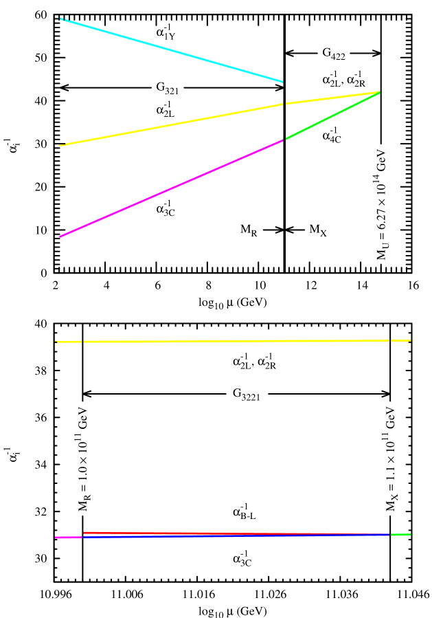
Figure 4: Plot showing the evolution of $\alpha_{i}^{-1}$ s in the SM phase, left-right phase upto $M_{U}$. The abscissa is $\ln(\mu)$, where $\mu$ initial is $M_{t}=173$ GeV and $M_{R}=10^{11}$ GeV in our case. The figure in the right shows explicitly the gauge coupling unification at $M_{U}\sim 10^{15}$ GeV.

If we start from $\mu=M_{T}=173$ GeV (where $n_{f}=6$) and fix $M_{R}=10^{11}$ GeV then the evolution of the gauge coupling constants are as given in Fig. 4. In the next phases the coupling constant evolution shows that at $M_{X}$ both $\alpha_{3C}$ and $\alpha_{B-L}$ unite to produce $\alpha_{4C}$. Fig. 4 shows that from $M_{X}$ on wards the development of $\alpha_{2L}$ and $\alpha_{2R}$ are identical. At around $M_{U}\sim 10^{15}$ GeV the gauge coupling constants unite. Our computational results show that the highest value of $M_{R}$ is just slightly above $10^{11}$ GeV. If $M_{R}$ is much above the above mentioned value then $M_{X}$ comes down and $M_{R}\geq M_{X}$.

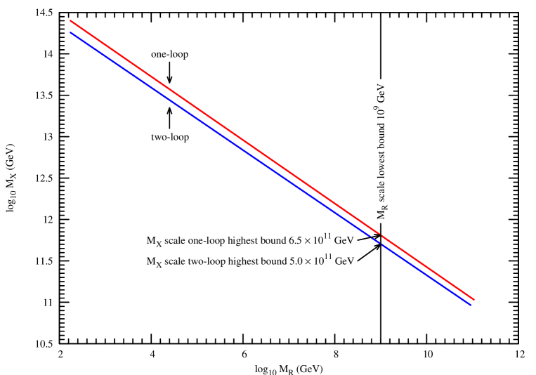
Figure 5: $M_{R}$ vs. $M_{X}$ shows lowest and highest bound.

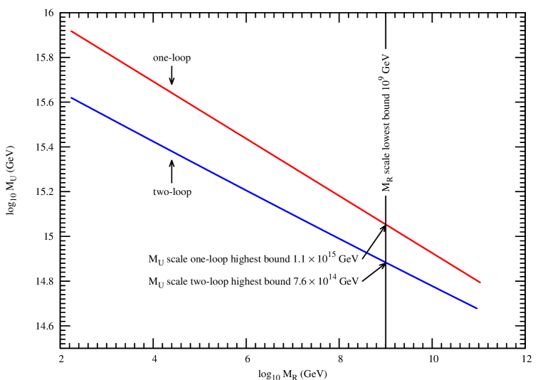
Figure 6: $M_{R}$ vs. $M_{U}$ shows lowest and highest bound.

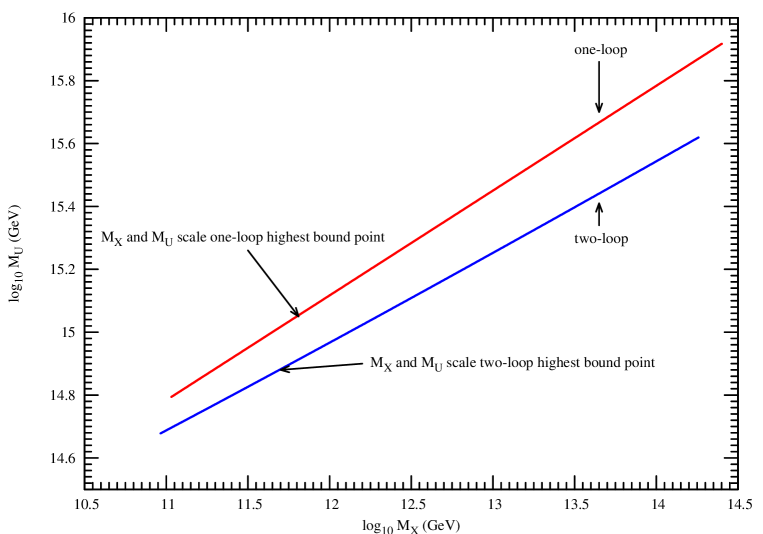
Figure 7: $M_{X}$ vs. $M_{U}$ shows lowest and highest bound.

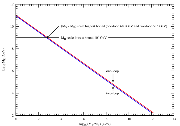
Figure 8: $M_{X}-M_{R}$ vs. $M_{X}$ shows how $M_{X}-M_{R}$ approaching zero.

In models with triplet Higgs scalars, it is possible to consider $M_{R}\geq M_{X}$. At the scale $M_{R}$, the group ${\rm SU(2)}_{R}$ is broken into ${\rm U(1)}_{R}$ and stays orthogonal to ${\rm SU(4)}_{C}$. Later when ${\rm SU(4)}_{C}$ is broken to ${\rm SU(3)}_{C}\times{\rm U(1)}_{B-L}$. Subsequently at a much lower scale the symmetry breaking, ${\rm U(1)}_{R}\times{\rm U(1)}_{B-L}\to{\rm U(1)}_{Y}$, takes place. However, this is not possible in scenarios with only doublet Higgs scalars, since the right-handed Higgs scalar doublet does not have any component with $B-L$ quantum number to be zero and hence it breaks ${\rm SU(2)}_{R}$ and ${\rm U}(1)_{B-L}$ simultaneously. As a result, the highest value of $M_{R}$ could be $10^{11}$ GeV. As we discussed earlier [14], the gauge coupling unification also requires a lower bound on $M_{R}>10^{9}$ GeV. From this lower (higher) bound for $M_{R}$, we estimated computationally higher (lower) bound for $M_{X}$ and $M_{U}$ as shown in Figs. 5, 6, 7. The lower and higher bounds for $M_{X}$ are $\sim 10^{11}$ GeV and $\sim 5\times 10^{11}$ GeV respectively. Also lower and higher bounds for $M_{U}$ are estimated as $5\times 10^{14}$ GeV and $\sim 10^{15}$ GeV respectively. In this regard it is important to note that the stability of the proton offers further constraints on the parameter space of their model, since the GUT scale is lower than most of the conventional models and is smaller than $10^{(}15)$GeV.

The difference between $M_{X}$ and $M_{R}$ can go up from 0 (i.e, $M_{R}=M_{X}$; no intermediate $G_{3221}$ symmetry) to $\sim 550$ GeV as shown in Fig. 8. This range of $M_{R}$ plays an important role for Yukawa coupling unification and leptogenesis in this model.

6 Yukawa coupling evolution

In sec. 4, Eq. (58) gives the only Yukawa couplings of our theory. Eq. (58) is valid in the SO(10) level. In the ${\rm G}_{422}$ level the Yukawa couplings will become:

$${\cal L}^{(4,2,2)}_{Y} = g^{\prime}S_{L}F^{(l)}_{L}\Phi^{*}_{L}+g^{\prime\prime}S_{L}F^{(r)}_{L}\Phi_{R}+M_{S}S_{L}S_{L}+h.c.\,.$$ (125)

The gauge transformation properties of the various fields, except $S_{L}$ which is a gauge singlet, are shown below:

$$\begin{array}[]{ccccc}F^{(l)}_{L}&\equiv&({\bf 4,2,1})\subset{\bf 16}&\equiv&\Gamma\,,\\ F^{(r)}_{L}&\equiv&({\bf\overline{4},1,2})\subset{\bf 16}&\equiv&\Gamma\,,\\ \Phi^{*}_{L}&\equiv&({\bf\overline{4},1,2})\subset{\overline{\bf 16}}&\equiv&{\Gamma^{\dagger}}\,,\\ \Phi_{R}&\equiv&({\bf 4,1,2})\subset{\overline{\bf 16}}&\equiv&{\Gamma^{\dagger}}\,.\end{array}$$ (130)

In the above equations $(\bf{x,y,z})$ designates the transformation properties under ${\rm G}_{422}$.

The Yukawa couplings in the ${\rm G}_{3221}$ phase is as:

$${\cal L}^{(3,2,2,1)}_{Y} = k^{\prime}_{(q)}S_{L}q_{L}H^{*}_{L}+k^{\prime}_{(l)}S_{L}\ell_{L}\chi^{*}_{L}+k^{\prime\prime}_{(q)}S_{L}(q_{R})^{c}H_{R}+k^{\prime\prime}_{(l)}S_{L}(\ell_{R})^{c}\chi_{R}$$ (131)

$$+\,M_{S}S_{L}S_{L}+h.c.\,.$$

The gauge transformation properties of $q_{L}$, $\ell_{L}$, $(q_{R})^{c}$, $(\ell_{R})^{c}$, $\chi^{*}_{L}$ and $\chi_{R}$ are specified in Eq. (18), Eq. (24) and Eq. (7). Here we specify the gauge transformation properties of the other two fields present in the above equation.

$$\begin{array}[]{cccccc}H^{*}_{L}&\equiv&({\bf\overline{3},2,1},-\frac{1}{3})\subset({\bf\overline{4},2,1})\subset{\bf\overline{16}}&\equiv&\Gamma^{\dagger}\,,\\ H_{R}&\equiv&({\bf 3,1,2},\frac{1}{3})\subset(\bf{4,1,2})\subset{\bf 16}&\equiv&\Gamma\,.\\ \end{array}$$ (134)

In the above equations $({\bf x,y,z},w)$ designates the ${\rm G}_{3221}$ transformation properties and $(\bf{x,y,z})$ designates the ${\rm G}_{422}$ transformation properties.

In the next stage, that is in the ${\rm G}_{321}$ phase, the Yukawa couplings look like:

$${\cal L}^{(3,2,1)}_{Y} = y_{(qL)}S_{L}Q_{L}T^{*}_{L}+y_{(lL)}S_{L}L_{L}h^{*}_{L}+y_{(u)}S_{L}(Q_{R})^{c}_{u}\,T^{(-)}_{R}$$ (135)

$$+\,y_{(d)}S_{L}(Q_{R})^{c}_{d}\,T^{(+)}_{R}+y_{(e)}S_{L}(e_{R})^{c}\,\phi^{(+)}_{*R}$$

$$+\,y_{(\nu)}S_{L}(\nu_{R})^{c}\,\phi^{(0)}_{*R}+M_{S}S_{L}S_{L}+h.c.\,.$$

Here the various standard model fermion fields transform under ${\rm G}_{321}$ as:

$$\begin{array}[]{cccccc}Q_{L}&\equiv&({\bf 3,2,}\frac{1}{3})\subset({\bf 3,2,1},\frac{1}{3})\subset({\bf 4,2,1})\subset{\bf 16}&\equiv&\Gamma\,,\\ L_{L}&\equiv&({\bf 1,2,}-1)\subset({\bf 1,2,1},-1)\subset({\bf 4,2,1})\subset{\bf 16}&\equiv&\Gamma\,,\\ (Q_{R})^{c}_{u}&\equiv&({\bf\overline{3},1},\frac{2}{3})\subset({\bf\overline{3},1,2},-\frac{1}{3})\subset({\bf\overline{4},1,2})\subset{\bf 16}&\equiv&\Gamma\,,\\ (Q_{R})^{c}_{d}&\equiv&({\bf\overline{3},1},-\frac{4}{3})\subset({\bf\overline{3},1,2},-\frac{1}{3})\subset({\bf\overline{4},1,2})\subset{\bf 16}&\equiv&\Gamma\,,\\ (e_{R})^{c}&\equiv&({\bf 1,1,}-2)\subset({\bf 1,1,2},1)\subset({\bf\overline{4},2,1})\subset{\bf 16}&\equiv&\Gamma\,,\\ (\nu_{R})^{c}&\equiv&({\bf 1,1,}0)\subset({\bf 1,1,2},1)\subset({\bf\overline{4},2,1})\subset{\bf 16}&\equiv&\Gamma\,.\\ \end{array}$$ (142)

Similarly the various Higgs fields transform as:

$$\begin{array}[]{cccccc}T^{*}_{L}&\equiv&({\bf\overline{3},2,}-\frac{1}{3})\subset(\bf{\overline{3},2,1,}{-\frac{1}{3}})\subset({\bf\overline{4},2,1})\subset{\bf\overline{16}}&\equiv&\Gamma^{\dagger}\,,\\ h^{*}_{L}&\equiv&({\bf 1,2,}1)\subset({\bf 1,2,1},1)\subset({\bf\overline{4},2,1})\subset{\bf\overline{16}}&\equiv&\Gamma^{\dagger}\,,\\ T^{(-)}_{R}&\equiv&({\bf 3,1},-\frac{2}{3})\subset({\bf 3,1,2},\frac{1}{3})\subset({\bf 4,1,2})\subset{\bf\overline{16}}&\equiv&\Gamma^{\dagger}\,,\\ T^{(+)}_{R}&\equiv&({\bf 3,1},\frac{4}{3})\subset({\bf 3,1,2},\frac{1}{3})\subset({\bf 4,1,2})\subset{\bf\overline{16}}&\equiv&\Gamma^{\dagger}\,,\\ \phi^{(+)}_{*R}&\equiv&({\bf 1,1,}2)\subset({\bf 1,1,2},-1)\subset({\bf 4,2,1})\subset{\bf\overline{16}}&\equiv&\Gamma^{\dagger}\,,\\ \phi^{(0)}_{*R}&\equiv&({\bf 1,1,}0)\subset({\bf 1,1,2},-1)\subset({\bf 4,2,1})\subset{\bf\overline{16}}&\equiv&\Gamma^{\dagger}\,.\\ \end{array}$$ (149)

In the above expressions the first triplet $({\bf x,y,}z)$ designates the transformation properties under ${\rm G}_{321}$, the next four numbers $({\bf x,y,z},w)$ designates the ${\rm G}_{3221}$ transformation properties and the triplet $(\bf{x,y,z})$ stands for the ${\rm G}_{422}$ transformation properties.

Now we give an order of magnitude estimation about the running of the effective top Yukawa coupling in our theory. From Eq. (61) it is seen that the effective top quark Yukawa coupling looks like $(\lambda^{\prime}_{\Gamma}v_{R}f^{2})/(8\pi^{2}M_{X})$. In the ${\rm G}_{321}$ phase it looks like $(\lambda^{\prime}_{\Gamma}v_{R}y_{(qL)}^{2})/(8\pi^{2}M_{X})$ in the convention adopted to name the Yukawa couplings in Eq. (135). Calling this effective coupling as $y_{t}$ it will evolve simply like:

$${dy_{t}\over dt} = \frac{y^{3}_{t}}{(16\pi^{2})}\,,$$ (150)

as in the standard-model up to the $M_{R}$ scale. The gauge and quartic coupling contributions will be negligible compared to $y_{t}$. Starting from the top-quark mass at the electroweak scale, the evolution equation gives the effective top-quark Yukawa coupling at the left-right symmetry breaking scale to be of the order of $0.76$ for $M_{R}\sim 10^{11}$ GeV. Since the effective coupling constant is a product of three couplings $(\lambda^{\prime}_{\Gamma}v_{R}y_{(qL)}^{2})/(8\pi^{2}M_{X})$ and if $v_{R}\sim M_{X}$ then each of these couplings can individually take values large enough as $3.9$. As a result the Yukawa sector becomes non-perturbative in the ${\rm G}_{3221}$ phase. But on the other hand if we have $(M_{X}/v_{R})\sim 10^{-2}$ then the situation changes. In this case the individual coupling becomes of the order of $0.84$ which implies the theory is still perturbative. $M_{X}$ can be the heavy gauge boson masses or the singlet fermion $S_{L}$ mass. The previous condition means that the heavy gauge bosons or the singlet fermion cannot be heavier than $10^{9}$ GeV in our theory if we take $M_{R}\sim 10^{11}$ GeV for a perturbative scenario in the Yukawa sector.

Above the left-right symmetry breaking scale $M_{R}$ up to the unification scale $M_{U}$, the coupling constants $\Lambda^{\prime}_{\Gamma}$ and $f$ will evolve separately. The separate Yukawa couplings remains finite up to the unification scale.

7 Leptogenesis

Since the neutrino masses now depend on the couplings with the singlets, there is no stringent restriction coming from the up quark masses. As a result, it may be possible to get large neutrino mixing angles. The right-handed neutrinos and the new singlet fermions can now decay into light leptons. The Majorana masses of the left-handed and right-handed singlets violate lepton numbers, which in turn can generate enough lepton asymmetry. Before the electroweak phase transition this asymmetry can then generate a baryon asymmetry of the universe [15]. Since there is no supersymmetry, the gravitino bounds are not present. The out-of-equilibrium condition can be satisfied near the GUT scale since the couplings are large to get the required neutrino mass with large see-saw scale. In this model there is another interesting feature that the singlets combine with the right-handed neutrinos to form pseudo-Dirac particles and hence resonant leptogenesis may also be possible [16, 17].

For leptogenesis, consider the interactions of Eq. (58). Unlike usual see-saw models with triplet Higgs scalars [18, 19], in this model the right-handed neutrinos cannot decay into left-handed neutrinos and Higgs bi-doublets dominantly. The simplest lepton number violating interactions come from the decays of $S_{i}$:

$$S_{i} \to \ell_{jL}+\chi^{*}_{L}\,,$$ (151)

$$\to {\ell_{jL}}^{c}+{\chi_{L}}\,.$$

The Majorana masses of $S_{i}$ allow the singlet to decay into both leptons and antileptons violating lepton number by two units. In the present model both $\ell_{L}$ and $\chi_{L}$ are very light and hence these decays are allowed.

For CP violation there are two types of one-loop diagrams which interferes with the tree-level diagrams for the decays of $S_{i}$. These are the vertex type diagrams of Fig. 9 and Fig. 10.

Figure 9: Vertex type diagrams interfering with tree level diagram. This is similar to the CP violation coming from the penguin diagram in K–decays.

Figure 10: Self energy diagram interfering with tree level diagram. This is similar to CP violation in $K-\bar{K}$ oscillation, entering in mass matrix of $S_{i}$.

The right-handed neutrinos do not take part in leptogenesis directly, but due to mixing of the right-handed neutrinos with the heavy singlets $S_{i}$, the right-handed neutrino decays also enter in the picture of leptogenesis. In the limit of $M_{S}\gg m_{R}$, the right-handed neutrinos and the $S_{i}$ are both heavy and distinct. In this case the amount lepton asymmetry due to CP violation is given by,

$$\delta=-{1\over 8\pi}\frac{M_{1}}{M_{2}}\frac{{\rm Im}[\sum_{\alpha}(k^{\prime\ast}_{(l)\,\alpha 1}k^{\prime}_{(l)\,\alpha 2})\sum_{\beta}(k^{\prime\ast}_{(l)\,\beta 1}k^{\prime}_{(l)\,\beta 2})]}{\sum_{\alpha}|k^{\prime}_{(l)\,\alpha 1}|^{2}}\,,$$ (152)

where we assumed that the mass matrix of $S_{i}$ are diagonal and the eigenvalues are hierarchical $M_{1}<M_{2}<M_{3}$ where $M_{i}$ are masses of $S_{i}$. We can write the effective lepton asymmetry as:

$$\epsilon=\delta\zeta\,,$$ (153)

where $\zeta$ is a suppression factor which depends on the amount of departure from equilibrium. The exact value of $\zeta$ can be obtained by solving the Boltzmann equation taking all the interactions into consideration. However, it is also possible to make an order of magnitude estimate for the amount of asymmetry, which will be very close to the actual value. Since $S_{1}$ is the lightest of the singlets, the decay of this singlet will be able to generate the lepton asymmetry. The asymmetry generated or washed out by the heavier ones $S_{2}$ or $S_{3}$ will be smeared out by the interactions of $S_{1}$ after $S_{2}$ and $S_{3}$ had decayed away. So, for an estimate we shall only consider the decays of $S_{1}$. This assumption is well justified when the singlets $S_{i}$ have a hierarchical mass structure.

The out-of-equilibrium condition is parametrized by:

$$\theta=\frac{1.7\sqrt{g_{*}}{T^{2}\over M_{P}}}{{|k^{\prime}_{(l)\,\alpha 1}|^{2}\over 16\pi}M_{1}}\,,\hskip 2.84544pt{\rm at}\quad T=M_{1}\,.$$ (154)

When $\theta>1$, there is no Boltzmann suppression of the generated asymmetry and the out-of-equilibrium condition is satisfied. In this case the generated asymmetry is given by $\delta$ and it is not washed out after it is created and one gets $\zeta=1$. However, if $\theta\gg 1$, then the interaction strength is so slow that the generated asymmetry can never reach the value $\delta$. Although the interactions cannot wash out the asymmetry after it is generated, the amount of asymmetry is less than $\delta$. In the case of $\theta<1$, the generated asymmetry is same as the CP asymmetry of $\delta$, but even after the asymmetry is created, the interaction remains strong enough to deplete the asymmetry. Although the depletion is exponentially fast, it cannot compete with the expansion of the universe for long and the final amount of asymmetry is not exponentially depleted. It was shown that [20] the suppression factor $\zeta$ is almost linearly proportional to $\theta$. In the present model we come across this last scenario.

In the present model $10^{9}~{}{\rm GeV}<M_{R}<10^{11}$ GeV. While a lower value of $M_{R}$ is preferable for out-of-equilibrium condition, since the Yukawa couplings grow very fast above the scale $M_{R}$ we have to consider the highest value of $M_{R}$. Taking the hierarchical structure of $S_{i}$, we consider the mass of the lightest singlet to be around $10^{10}$ GeV. Taking $M_{1}\sim 10^{10}$ GeV, $g_{*}\sim 10^{2}$ and $k^{\prime}_{(l)\,\alpha 1}\sim 1$ we find that $\theta$ is much lower than 1, which gives a strong suppression factor of $\zeta\sim 10^{-7}$. On the other hand the Yukawa couplings in this model comes out to be of the order of 1 and hence we get a large enhancement in the CP asymmetry and $\delta$ in our case can be as large as $10^{-2}$ and so the lepton asymmetry parameter $\epsilon\sim 10^{-9}$.

At this stage, $\Delta B=0$ and $\Delta L$ is given by $\delta$. Thus

$$\Delta(B-L)=\epsilon\,.$$ (155)

The final baryon asymmetry after the electroweak phase transition is thus given by,

$${n_{B}\over s}={1\over 3}\Delta(B-L)={\epsilon\over 3}\sim 10^{-10}\,.$$ (156)

In the case of $M_{S}\ll m_{R}$, the right-handed neutrinos and the $S_{i}$ singlets of every generation are almost degenerate. The mass splitting between the states $\nu_{iR}$ and $S_{i}$ with mass $m_{R}$ is of the order of $M_{S}$. Although $S_{i}$ decays will now generate a lepton asymmetry, both the heavy mass eigenstates contain the states $S_{i}$. As a result, when these two almost degenerate states decay, there may be resonant leptogenesis (which will however require new interactions and fine-tuning) and hence the scale of leptogenesis could be very low. For the present scenario since $M_{R}$ and hence $M_{1}$ cannot be much lower, this is not important and hence we shall not discuss it in any further detail.

8 Summary

In conclusion, we constructed an SO(10) GUT without any Higgs bi-doublets. All the symmetry breaking could be achieved by only two Higgs scalars, a ${\bf 210}$ and a ${\bf 16}$. By including a massive singlet fermion per generation we break chiral symmetry which can then give masses to all the fermions radiatively without introducing any new scalar fields. All fermion masses have the same see-saw form. The spontaneous parity breaking plays a crucial role in breaking the left-handed and right-handed SU(2) groups at two widely different scales and also giving masses to the left-handed neutrinos in this scenario. The spontaneous breaking of an ungauged discrete symmetry, the D-parity, which is a special feature of this model may cause formation of very heavy domain walls of GUT-scale mass. Since the GUT scale in the model is rather low $(\sim 10^{15}$ GeV), some of the parameters of the model may have to be constrained further to prevent fast proton decay. These features require further study and will be taken up in future. The model allows large neutrino mixing and required neutrino masses. The baryon asymmetry of the universe can be explained through leptogenesis.

References

[1]K.S. Babu and R.N. Mohapatra, Phys.Rev.Lett. 70,
2845 (1993).
[2] B. Bajc, G. Senjanović and F. Vissani,
Phys.Rev.Lett. 90, 051802 (2003);
H.S. Goh, R.N. Mohapatra and S.P. Ng,
Phys.Lett. B570, 215 (2003) and
Phys.Rev. D68, 115008 (2003);
S. Bertolini, M. Frigerio and M. Malinsky, Phys.Rev. D70, 095002 (2004).
[3] T. Clark, T. Kuo and N. Nakagawa,
Phys.Lett. B115, 26 (1982);
C.S. Aulakh and R.N. Mohapatra, Phys.Rev. D28, 217 (1983);
C.S. Aulakh, B. Bajc, A. Melfo, G. Senjanović and F. Vissani,
Phys.Lett. B588, 196 (2004);
T. Fukuyama, A. Ilakovic, T. Kikuchi, S. Meljanac and
N. Okada, Eur.Phys.J. C42, 191 (2005) and
J.Math.Phys. 46, 033505 (2005);
C.S. Aulakh and A. Giridhar, Nucl.Phys. B711, 275 (2005).
[5] S. Rajpoot, Phys.Rev. D22, 2244 (1980);
R.N. Mohapatra, Phys.Rev. D34, 3457 (1986);
A. Font, L.E. Ibáñez and F. Quevedo, Phys.Lett. B228, 79 (1989);
S.P. Martin, Phys.Rev. D46, 2769 (1992);
C.S. Aulakh, K. Benakli and G. Senjanović, Phys.Rev.Lett. 79, 2188 (1997);
C.S. Aulakh, A. Melfo, A. Rašin and G. Senjanović, Phys.Lett. B459, 557 (1999)
and
Nucl.Phys. B597, 89 (2001);
T. Hambye and G. Senjanović, Phys.Lett. B582, 73 (2004);
G. D’Ambrosio, T. Hambye, A. Hektor, M. Raidal and A. Rossi,
Phys.Lett. B604, 199 (2004).
[6] J.C. Pati and A. Salam, Phys.Rev. D10, 275 (1974);
R.N. Mohapatra and J.C. Pati, Phys.Rev. D11, 566 (1975); ibid., 2558 (1975);
G. Senjanović and R.N. Mohapatra, Phys.Rev. D12, 1502 (1975).
[7]
B.R. Desai, G. Rajasekaran and U. Sarkar, Phys.Lett. B626, 167 (2005).
[8] A. Davidson and K.C. Wali, Phys.Rev.Lett. 59, 393 (1987);
S. Rajpoot, Phys.Rev. D36, 1479 (1987).
[9] D. Chang and R.N. Mohapatra, Phys.Rev.Lett. 58, 1600 (1987);
B.S. Balakrishna, Phys.Rev.Lett. 60, 1602 (1988);
K.S. Babu and R.N. Mohapatra, Phys.Rev.Lett. 62, 1079 (1989) and
Phys.Rev. D41, 1286 (1990).
[10]
B. Brahmachari, E. Ma and U. Sarkar,
Phys.Rev.Lett. 91, 011801 (2003);
U. Sarkar,
Phys.Lett. B622, 118 (2005).
[11] D.R.T. Jones, Phys.Rev. D25, 581 (1982).
[12] S. Eidelman et al., Phys.Lett. B592, 1 (2004).
[13] The 2005 web update of the Particle Listings: http://pdg.lbl.gov/
[14] P. Langacker and M.X. Luo, Phys.Rev. D44, 817 (1991);
B. Brahmachari, U. Sarkar and K. Sridhar, Phys.Lett. B297, 105 (1992).
[15] M. Fukugita and T. Yanagida, Phys.Lett. B174, 45 (1986).
[16] M. Flanz, E.A. Paschos, and U. Sarkar, Phys.Lett.
B345, 248 (1995);
L. Covi, E. Roulet and F. Vissani, Phys.Lett. B384, 169 (1996);
M. Flanz, E.A. Paschos, U. Sarkar and
J. Weiss, Phys.Lett. B389, 693 (1996);
A. Pilaftsis, Nucl.Phys. B504, 61 (1997) and
Phys.Rev. D56, 5431 (1997);
W. Buchmüller and M. Plümacher, Phys.Lett. B431, 354 (1998);
A. Pilaftsis, Int.J.Mod.Phys. A14, 1811 (1999);
A. Pilaftsis and T.E.J. Underwood, Nucl.Phys. B692, 303 (2004);
T. Hambye, J. March-Russell and S.M. West, JHEP 0407, 070 (2004).
[17] C.H. Albright and
S.M. Barr, Phys.Rev. D69, 073010 (2004) and
Phys.Rev. D70, 033013 (2004).
[18] E. Ma and U. Sarkar, Phys.Rev.Lett. 80, 5716 (1998);
G. Lazarides and Q. Shafi, Phys.Rev. D58, 071702 (1998);
W. Grimus, R. Pfeiffer and T. Schwetz, Eur.Phys.J. C13, 125 (2000);
E. Ma, M. Raidal and U. Sarkar, Phys.Rev.Lett. 85,
3769 (2000) and
Nucl.Phys. B615, 313 (2001);
T. Hambye, E. Ma and U. Sarkar, Nucl.Phys. B602, 23 (2001);
T. Hambye, M. Raidal and A. Strumia, Phys.Lett. B632, 667 (2006).
[19] A. Acker, H. Kikuchi, E. Ma and U. Sarkar,
Phys.Rev. D48, 5006 (1993);
P.J. O’Donnell and U. Sarkar, Phys.Rev.
D49, 2118 (1994);
M. Plumacher, Z.Phys. C74, 549 (1997);
T. Hambye and G. Senjanović, Phys.Lett. B582, 73 (2004);
S. Antusch and S.F. King, Phys.Lett. B597, 199 (2004);
Narendra Sahu and S. Uma Sankar, Nucl.Phys. B724, 329 (2005);
K.S. Babu, A. Bachri and H. Aissaoui, Nucl.Phys. B738, 76 (2006).
[20] J. Faridani, S. Lola, P.J. O’Donnell and U. Sarkar,
Eur.Phys.J. C7, 543 (1999).