Threshold Resummation for $W$-Boson Production at RHIC

Abstract

We study the resummation of large logarithmic perturbative corrections to the partonic cross sections relevant for the process $pp\to W^{\pm}X$ at the BNL Relativistic Heavy Ion Collider (RHIC). At RHIC, polarized protons are available, and spin asymmetries for this process will be used for precise measurements of the up and down quark and anti-quark distributions in the proton. The corrections arise near the threshold for the partonic reaction and are associated with soft-gluon emission. We perform the resummation to next-to-leading logarithmic accuracy, for the rapidity-differential cross section. We find that resummation leads to relatively moderate effects on the cross sections and spin asymmetries.

I Introduction

The exploration of the spin structure of the nucleon has by now become a classic topic of nuclear and particle physics. Most of our knowledge so far comes from spin-dependent deeply-inelastic scattering (DIS) which has produced spectacular results reviews , the single most important one being that the total quark spin contribution to the nucleon spin is only about $20-25\%$. This has led to a new generation of experiments that aim at further unraveling the spin structure of the nucleon. Among these are experiments at the Relativistic Heavy Ion Collider (RHIC) at BNL. Here, a new method is used, namely to study collisions of two polarized protons rhicrev . This allows in particular clean probes of the polarized gluon distribution in the proton, whereby one is hoping to learn about the contribution of gluons to the proton spin.

DIS has given us exciting information on the spin-dependent quark and anti-quark distributions $\Delta q(x,\mu^{2})$, $\Delta\bar{q}(x,\mu^{2})$, where $\Delta q(x,\mu^{2})\equiv q^{\uparrow}(x,\mu^{2})-q^{\downarrow}(x,\mu^{2})$ with $q^{\uparrow}(x,\mu^{2})$ ($q^{\downarrow}(x,\mu^{2})$) denoting the distributions of quarks with positive (negative) helicity and light-cone momentum fraction $x$ in a proton with positive helicity, at factorization scale $\mu$. Inclusive DIS via photon exchange, however, gives access only to the combinations $\Delta q+\Delta\bar{q}$. In order to understand the proton helicity structure in detail, one would like to learn about the various quark and anti-quark densities, $\Delta u,\Delta\bar{u},\Delta d,\Delta\bar{d},\Delta s,\Delta\bar{s}$, individually. This is for example relevant for comparisons to models of nucleon structure which generally make clear qualitative predictions about, for example, the flavor asymmetry $\Delta\bar{u}-\Delta\bar{d}$ in the proton sea su2 . These predictions are often related to fundamental concepts such as the Pauli principle: since the proton has two valence-$u$ quarks which primarily spin along with the proton spin direction, $u\bar{u}$ pairs in the sea will tend to have the $u$ quark polarized opposite to the proton. Hence, if such pairs are in a spin singlet, one expects $\Delta\bar{u}>0$ and, by the same reasoning, $\Delta\bar{d}<0$. Such questions become all the more exciting due to the fact that rather large unpolarized asymmetries $\bar{u}-\bar{d}\neq 0$ have been observed in DIS and Drell-Yan measurements dysu2 ; dysu21 ; dysu22 .

There are two known ways to distinguish between quark and anti-quark polarizations experimentally, and also to achieve at least a partial flavor separation. Semi-inclusive measurements in DIS are one possibility, explored by SMC smc and, more recently and with higher precision, by Hermes hermesdq . Results are becoming available now also from the Compass experiment compass , and measurements have been proposed for the Jefferson Laboratory jlab . One detects a hadron $h$ in the final state, so that instead of $\Delta q+\Delta\bar{q}$ the polarized DIS cross section becomes sensitive to $\;\Delta q(x)\,D_{q}^{h}(z)+\Delta\bar{q}(x)\,D_{\bar{q}}^{h}(z)$, for a given quark flavor. Here, the $D_{i}^{h}(z)$ are fragmentation functions, with $z$ denoting the fraction of the momentum of the struck quark transfered to the hadron. The dependence on the details of the fragmentation process limits the accuracy of this method. There is much theory activity currently on SIDIS, focusing on next-to-leading order (NLO) corrections, target fragmentation, and higher twist contributions sidis .

The other method to learn about the $\Delta q$ and $\Delta\bar{q}$ will be used at RHIC. Here one considers spin asymmetries in the production of $W^{\pm}$ bosons BOURRELY93 . Because of the violation of parity in the coupling of $W$ bosons to quarks and anti-quarks, single-longitudinal spin asymmetries, defined as

$$A_{L}\equiv\frac{{\rm d}\sigma^{++}+{\rm d}\sigma^{+-}-{\rm d}\sigma^{-+}-{\rm d}\sigma^{--}}{{\rm d}\sigma^{++}+{\rm d}\sigma^{+-}+{\rm d}\sigma^{-+}+{\rm d}\sigma^{--}}\equiv\frac{{\rm d}\Delta\sigma}{{\rm d}\sigma}\;,$$ (1)

can be non-vanishing. Here the $\sigma$ denote cross sections for scattering of protons with definite helicities as indicated by the superscripts; as one can see, we are summing over the helicities of the second proton, which leads to the single-spin process $\vec{p}p\to W^{\pm}X$. Since the $W$ mass sets a large momentum scale in the process, the cross sections factorize into convolutions of parton distribution functions and partonic hard-scattering cross sections. The latter are amenable to QCD perturbation theory, the lowest-order reaction being the “Drell-Yan” process $q\bar{q}^{\prime}\to W^{\pm}$. For produced $W^{+}$, the dominant contributions come from $u\bar{d}\to W^{+}$, and the spin asymmetry is approximately given by rhicrev ; craigie83 ; BOURRELY93

$$A_{L}^{W^{+}}=\frac{\Delta u(x_{1}^{0},M_{W}^{2})\bar{d}(x_{2}^{0},M_{W}^{2})-\Delta\bar{d}(x_{1}^{0},M_{W}^{2})u(x_{2}^{0},M_{W}^{2})}{u(x_{1}^{0},M_{W}^{2})\bar{d}(x_{2}^{0},M_{W}^{2})+\bar{d}(x_{1}^{0},M_{W}^{2})u(x_{2}^{0},M_{W}^{2})}\;.$$ (2)

Here, as indicated, the parton distributions will be probed at a scale $\sim M_{W}$, with $M_{W}$ the $W$ mass, and the momentum fractions $x_{1}^{0}$ and $x_{2}^{0}$ are related to the rapidity $\eta$ of the $W^{+}$ by

$$x_{1,2}^{0}=\frac{M_{W}}{\sqrt{S}}\,e^{\pm\eta}\;,$$ (3)

where $\sqrt{S}$ is the $pp$ center-of-mass energy which at RHIC is 200 or 500 GeV. Note that $\eta$ is counted positive in the forward region of the polarized proton. From Eq. (2) it follows that at large $\eta$, where $x_{1}^{0}\sim 1$ and $x_{2}^{0}\ll 1$, the asymmetry will be dominated by the valence distribution probed at $x_{1}^{0}$, and hence give direct access to $\Delta u(x_{1}^{0},M_{W}^{2})/u(x_{1}^{0},M_{W}^{2})$. Likewise, for large negative $\eta$, $A_{L}^{W^{+}}$ is given by $-\Delta\bar{d}(x_{1}^{0},M_{W}^{2})/\bar{d}(x_{1}^{0},M_{W}^{2})$. For negatively charged $W$ bosons, one finds correspondingly sensitivity to $\Delta d(x_{1}^{0},M_{W}^{2})/d(x_{1}^{0},M_{W}^{2})$ and $-\Delta\bar{u}(x_{1}^{0},M_{W}^{2})/\bar{u}(x_{1}^{0},M_{W}^{2})$ at large positive and negative $W$ rapidities, respectively. This is the key idea behind the planned measurements of $\Delta u,\Delta\bar{u},\Delta d,\Delta\bar{d}$ at RHIC.

In practice, a significantly more involved strategy needs to be used in order to really relate the single-longitudinal spin asymmetries to the polarized quark and anti-quark densities. Partly, this is an experimental issue: the detectors at RHIC are not hermetic, which means that missing-momentum techniques for the charged-lepton neutrino ($l\nu_{l}$) final states cannot be straightforwardly used to detect the $W$ and reconstruct its rapidity. There are, however, workarounds to this problem. One is to assume that the $W$ is dominantly produced with near-zero transverse momentum, in which case one can relate the measured rapidity of the charged lepton to that of the $W$, up to an irreducible sign ambiguity bland ; NadYuan2 . Ultimately, it may then become more expedient not even to consider the $W$ rapidity, but to formulate all observables directly in terms of the charged-lepton rapidity. This approach has been studied in detail in NadYuan2 ; NadYuan1 . It was found that despite the fact that the interpretation of the spin asymmetries in terms of the $\Delta u,\Delta\bar{u},\Delta d,\Delta\bar{d}$ becomes more involved, there still is excellent sensitivity to them. Contributions by $Z$ bosons need to be taken into account as well. Very recently, it has also been proposed NadTalk to use hadronic $W$ decays in the measurements of $A_{L}$. These have the advantage that one just needs to look for events with two hadronic jets. A potential drawback is that, while the QCD two-jet background cancels in the parity-violating numerator of $A_{L}$, it does contribute to the denominator and therefore will likely reduce the size of the spin asymmetries.

There are also theoretical issues that modify the picture related to Eq. (2) described above. There are for example Cabibbo-suppressed contributions. It is relatively straightforward to take these into account, even though one needs to keep in mind that they involve the polarized and unpolarized strange quark distributions. More importantly, there are higher-order QCD corrections to the leading order (LO) process $q\bar{q}^{\prime}\to W^{\pm}$. At next-to-leading order, one has the partonic reactions $q\bar{q}^{\prime}\to W^{\pm}g$ and $qg\to W^{\pm}q^{\prime}$. For the unpolarized and the single-longitudinal spin cases, the cross sections for these have been given and studied in Refs. aem ; kubar and ratcliffe ; weber ; weberqt ; kamal ; tgdy ; gehrmann ; grh , respectively. In the present paper, we will improve the theoretical framework by going beyond NLO and performing a resummation of certain logarithmically enhanced terms in the partonic cross sections to all orders in perturbation theory.

The corrections we are considering arise near “partonic threshold”, when the initial partons have just enough energy to produce the $W$ boson. Here the phase space available for real-gluon radiation vanishes, while virtual corrections are fully allowed. The cancellation of infrared singularities between the real and virtual diagrams then results in large logarithmic “Sudakov” corrections to the LO $q\bar{q}^{\prime}$ cross section. For example, for the cross section integrated over all rapidities of the $W$, the most important logarithms (the “leading logarithms” (LL)) take the form $\alpha_{s}^{k}[\ln^{2k-1}(1-z)/(1-z)]_{+}$ at the $k$th order of perturbation theory, where $z=M_{W}^{2}/\hat{s}$ with $\hat{s}$ the partonic center-of-mass energy, and $\alpha_{s}$ is the strong coupling. The “$+$”-distribution is defined in the usual way and regularizes the infrared behavior $z\to 1$. Subleading logarithms are down by one or more powers of the logarithm and are referred to as “next-to-leading logarithms” (NLL), and so forth. Because of the interplay of the partonic cross sections with the steeply falling parton distributions, the threshold regime can make a substantial contribution to the cross section even if the hadronic process is relatively far from threshold, that is, even if $M_{W}^{2}/S\ll 1$. If $M_{W}^{2}/S\sim 1$, the threshold region will completely dominate the cross section. This is expected to be the case for $W$ production at the RHIC energies, in particular at $\sqrt{S}=200$ GeV. Sufficiently close to partonic threshold, the perturbative series will be only useful if the large logarithmic terms are taken into account to all orders in $\alpha_{s}$. This is achieved by threshold resummation.

Drell-Yan type processes have been the first for which threshold resummation was derived. The seminal work in dyresum ; dyresum2 has been the starting point for the developments of related resummations for many hard processes in QCD f2 . The resummation for Drell-Yan is now completely known to next-to-next-to-leading logarithmic (NNLL) accuracy f1 . In this paper we will, however, perform the resummation only at NLL level. Since the strong coupling at scale $M_{W}$ is relatively small, we expect this to be completely sufficient for a good theoretical description. In addition, away from the threshold region, one needs to match the resummed calculation to the available fixed-order one. In our case of single-spin production of $W$’s, this is NLO. A consistent matching of a NNLL resummation would require matching to NNLO, which is not yet available.

As we discussed above, of particular interest at RHIC for determining the spin-dependent quark and anti-quark densities are the rapidity distributions of the $W$ bosons. In order to present phenomenology relevant for RHIC, we will therefore perform the resummation for the rapidity-dependent cross sections. Note that we will concentrate only on the case of the distributions in $W$-boson rapidity; from the earlier discussion it follows that for future studies it would be even more desirable to consider the distributions in charged-lepton rapidities. To treat the resummation at fixed $W$ rapidity, we will employ the technique developed in sv . This entails to use Mellin moments in $\tau=M_{W}^{2}/S$ of the cross section, as is customary in threshold resummation, but also a Fourier transform in rapidity. In sv , this method was applied to the prompt-photon cross section. For the case of the Drell-Yan cross section it simplifies considerably. We note that techniques for the threshold resummation of the Drell-Yan cross section at fixed rapidity were also briefly discussed in LaenenSterman . We verify the main result of that paper, and for the first time, present phenomenological results for this case.

Before turning to the main part of the paper, we mention that important work on another type of resummation of the $W$ production cross sections at RHIC has been performed in the literature, namely for the transverse-momentum distribution ($p_{T}$) of the $W$’s weberqt ; NadYuan2 ; NadYuan1 . At lowest order, the $W$ is produced with vanishing transverse momentum. Gluon radiation generates a recoil transverse momentum. By a similar reasoning as above, when $p_{T}$ tends to zero, large logarithmic corrections develop in the $p_{T}$ spectrum of the $W$’s. These can be resummed as well, which was studied for the case of RHIC in great detail in weberqt ; NadYuan2 ; NadYuan1 . For the total or the rapidity-differential $W$ cross section we are interested in, $p_{T}$ is integrated, and the associated large logarithms turn partly into threshold logarithms and partly into nonlogarithmic terms. Therefore, the threshold logarithms we are considering here become the main source of large corrections to the cross section. We note that ultimately it would be desirable to perform a “joint” resummation of the $p_{T}$ and threshold logarithms, as developed in Ref. LSV .

The remainder of this paper is organized as follows. In Section II we present general formulas for the single-spin cross section for $W$ production as a function of rapidity, and also discuss the NLO corrections. In Section III, we give details of the Mellin and Fourier transforms that are useful in achieving threshold resummation of the rapidity-dependent cross section. The next two sections provide the formulas for the resummed cross sections. In Section VI we present our numerical results for RHIC.

II Cross section for $W$ production in $\vec{p}p$ collisions

The rapidity-differential Drell-Yan cross section for $W^{\pm}$ production in singly-polarized $pp$ collisions can be written as gehrmann

$$\frac{{\rm d}\Delta\sigma}{{\rm d}\eta} = {\cal N}\sum_{i,j}\int_{x_{1}^{0}}^{1}{\rm d}x_{1}\int_{x_{2}^{0}}^{1}{\rm d}x_{2}\,\Delta{\cal D}_{ij}\left(x_{1},x_{2},x_{1}^{0},x_{2}^{0},\alpha_{s}(\mu^{2}),\frac{M_{W}^{2}}{\mu^{2}}\right)\,\Delta f_{i}(x_{1},\mu^{2})\,f_{j}(x_{2},\mu^{2})$$ (4)

$$= {\cal N}\sum_{i,j}c_{ij}\int_{x_{1}^{0}}^{1}{\rm d}x_{1}\int_{x_{2}^{0}}^{1}{\rm d}x_{2}$$

$$\times\Bigg{\{}D_{q\bar{q}}\left(x_{1},x_{2},x_{1}^{0},x_{2}^{0},\alpha_{s}(\mu^{2}),\frac{M_{W}^{2}}{\mu^{2}}\right)\Big{[}-\Delta q_{i}(x_{1},\mu^{2})\bar{q}_{j}(x_{2},\mu^{2})+\Delta\bar{q}_{i}(x_{1},\mu^{2})q_{j}(x_{2},\mu^{2})\Big{]}$$

$$+\Delta D_{gq}\left(x_{1},x_{2},x_{1}^{0},x_{2}^{0},\alpha_{s}(\mu^{2}),\frac{M_{W}^{2}}{\mu^{2}}\right)\Delta G(x_{1},\mu^{2})\left[q_{j}(x_{2},\mu^{2})-\bar{q}_{j}(x_{2},\mu^{2})\right]$$

$$+D_{qg}\left(x_{1},x_{2},x_{1}^{0},x_{2}^{0},\alpha_{s}(\mu^{2}),\frac{M_{W}^{2}}{\mu^{2}}\right)\left[-\Delta q_{i}(x_{1},\mu^{2})+\Delta\bar{q}_{i}(x_{1},\mu^{2})\right]G(x_{2},\mu^{2})\Bigg{\}}\;,$$

where the $\Delta f_{i}$, $f_{j}$ are the polarized and unpolarized parton distributions, respectively, and where in the second equation we have written out explicitly the various contributions that are possible through NLO. Furthermore, the normalization factor ${\cal N}$ is given by

$${\cal N}=\frac{\pi G_{F}M_{W}^{2}\sqrt{2}}{3S}\;,$$ (5)

with the Fermi constant $G_{F}$, and $c_{ij}$ are the coupling factors for $W^{\pm}$ bosons,

$$c_{ij}=|V_{ij}|^{2}$$ (6)

with $V_{ij}$ the CKM mixing factors for the quark flavors $i,j$. $\mu\sim M_{W}$ denotes the renormalization/factorization scales which we take to be equal. $x_{1}^{0}$ and $x_{2}^{0}$ have been defined above in Eq. (3).

The $D_{q\bar{q}}$, $\Delta D_{gq}$, $D_{qg}$ in Eq. (4) are the hard-scattering functions. For the single-spin cross section, always one initial parton is unpolarized. Therefore, thanks to helicity conservation in QCD and the $V-A$ structure of the $Wq\bar{q}^{\prime}$ vertex, when the polarized parton is a quark, one finds that the spin-dependent partonic cross section is the negative of the unpolarized one. We have therefore omitted the $\Delta$’s in these cases and only included a $\Delta$ for the case of an initial polarized gluon where there is no trivial relation between the polarized and the unpolarized cross sections. Each of the hard-scattering functions $D_{ij}$ (or $\Delta D_{ij}$) is a perturbative series in the strong coupling $\alpha_{s}(\mu^{2})$:

$$D_{ij}\left(x_{1},x_{2},x_{1}^{0},x_{2}^{0},\alpha_{s}(\mu^{2}),\frac{M_{W}^{2}}{\mu^{2}}\right) = D_{ij}^{(0)}\left(x_{1},x_{2},x_{1}^{0},x_{2}^{0}\right)$$ (7)

$$+\frac{\alpha_{s}(\mu^{2})}{2\pi}D_{ij}^{(1)}\left(x_{1},x_{2},x_{1}^{0},x_{2}^{0},\frac{M_{W}^{2}}{\mu^{2}}\right)+\ldots\;.$$

Only the $q\bar{q}^{\prime}$ process has a lowest-order [${\cal O}(\alpha_{s}^{0})$] contribution:

$$D_{q\bar{q}}^{(0)}(x_{1},x_{2},x_{1}^{0},x_{2}^{0}) = \delta(x_{1}-x_{1}^{0})\,\delta(x_{2}-x_{2}^{0})\;,$$

$$\Delta D_{gq}^{(0)}(x_{1},x_{2},x_{1}^{0},x_{2}^{0}) = D_{qg}(x_{1},x_{2},x_{1}^{0},x_{2}^{0})\;=\;0\;.$$ (8)

The NLO hard-scattering functions have rather lengthy expressions which have been derived in Refs. kubar ; weber ; tgdy . For the reader’s convenience we collect them in the Appendix. As can be seen from Eqs. (8), (35)-(39), the coefficients contain distributions in $(x_{1}-x_{1}^{0})$ and $(x_{2}-x_{2}^{0})$. These are the terms addressed by threshold resummation. More precisely, it turns out that only products of two “plus”-distributions, or a product of a “plus”-distribution and a delta-function, are leading near threshold. This occurs only for the coefficient $D_{q\bar{q}}$. To be able to write down the resummed expressions for arbitrary rapidity, we need to take suitable integral transforms, to which we shall turn now.

III Mellin and Fourier transforms, and threshold limit

Consider the production of a $W$ boson through a single generic partonic reaction involving initial partons $i$ and $j$. We define a double transform of the cross section, in terms of a Mellin transform in $\tau=M_{W}^{2}/S$ and a Fourier transform in the rapidity of the $W$ boson:

$$\Delta\tilde{\sigma}(N,M) \equiv \int_{0}^{1}d\tau\,\tau^{N-1}\int_{-\ln\frac{1}{\sqrt{\tau}}}^{\ln\frac{1}{\sqrt{\tau}}}d\eta\,{\mathrm{e}}^{iM\eta}\,{d\Delta\sigma\over d\eta}$$

$$=\,{\cal N}\int_{0}^{1}dx_{1}x_{1}^{N+iM/2}\Delta f_{i}(x_{1})\int_{0}^{1}dx_{2}\,x_{2}^{N-iM/2}f_{j}(x_{2})\int_{0}^{1}dz\,z^{N-1}\int_{-\ln\frac{1}{\sqrt{z}}}^{\ln\frac{1}{\sqrt{z}}}d{\hat{\eta}}\,{\mathrm{e}}^{iM{\hat{\eta}}}\,\Delta{\cal D}_{ij}\;.$$

Here we have suppressed the argument of the partonic cross section as well as the scale dependence of the parton distributions. We have introduced parton level variables $z=\tau/x_{1}x_{2}$ and ${\hat{\eta}}=\eta-{1\over 2}\ln(x_{1}/x_{2})$. Each of the functions $\Delta{\cal D}_{ij}$ is of the form $(x_{1}x_{2})^{-1}$ times a function of $x_{1}^{0}/x_{1}$ and $x_{2}^{0}/x_{2}$ only. Defining the moments

$$f^{N}(\mu^{2})\equiv\int_{0}^{1}dx\,x^{N-1}f(x,\mu^{2})\;,\\$$

of the parton densities, and

$$\Delta\tilde{{\cal D}}_{ij}(N,M)\equiv\int_{0}^{1}dz\,z^{N-1}\int_{-\ln\frac{1}{\sqrt{z}}}^{\ln\frac{1}{\sqrt{z}}}d{\hat{\eta}}\,{\mathrm{e}}^{iM{\hat{\eta}}}\,\left(x_{1}x_{2}\Delta{\cal D}_{ij}\right)\;,$$ (10)

we therefore have:

$$\Delta\tilde{\sigma}(N,M)={\cal N}\,\Delta f_{i}^{N+iM/2}\,f_{j}^{N-iM/2}\,\Delta\tilde{{\cal D}}_{ij}(N,M)\;.$$ (11)

At lowest order,

$$x_{1}x_{2}D_{q\bar{q}}^{(0)}\left(x_{1},x_{2},x_{1}^{0},x_{2}^{0}\right)=x_{1}x_{2}\delta(x_{1}-x_{1}^{0})\,\delta(x_{2}-x_{2}^{0})=\delta\left(1-\sqrt{z}{\mathrm{e}}^{\hat{\eta}}\right)\,\delta\left(1-\sqrt{z}{\mathrm{e}}^{-\hat{\eta}}\right)\;,$$ (12)

and we find

$$\int_{0}^{1}dz\,z^{N-1}\int_{-\ln\frac{1}{\sqrt{z}}}^{\ln\frac{1}{\sqrt{z}}}d{\hat{\eta}}\,{\mathrm{e}}^{iM{\hat{\eta}}}\,\delta\left(1-\sqrt{z}{\mathrm{e}}^{\hat{\eta}}\right)\delta\left(1-\sqrt{z}{\mathrm{e}}^{-\hat{\eta}}\right)\,=\,\int_{0}^{1}dz\,z^{N-1}\,2\cos\left(M\ln\frac{1}{\sqrt{z}}\right)\,\delta(1-z)\;.$$ (13)

As one can see, a $\delta(1-z)$ emerges, as expected from the well-known expression for the rapidity-integrated LO Drell-Yan cross section aem . Beyond LO, a closed calculation of the double moments $\Delta\tilde{{\cal D}}_{ij}(N,M)$ is very difficult. For example, at NLO, one would need to use the expressions given in Eqs. (35)-(39) and take the moments in $N$ and $M$. Fortunately, a great simplification occurs in the near-threshold limit. Equation (13) shows that the partonic threshold, after taking Fourier moments in rapidity, is reached at $z=1$. In Mellin-moment space, this corresponds to the large-$N$ limit. Even though the Cosine factor is obviously unity in conjunction with the term $\delta(1-z)$, it is generic, as we will now see.

At NLO, one finds from Eqs. (35)-(39) the following structure near threshold:

$$\int_{0}^{1}dz\,z^{N-1}\int_{-\ln\frac{1}{\sqrt{z}}}^{\ln\frac{1}{\sqrt{z}}}d{\hat{\eta}}\,{\mathrm{e}}^{iM{\hat{\eta}}}\,x_{1}x_{2}D_{q\bar{q}}^{(1)}\left(x_{1},x_{2},x_{1}^{0},x_{2}^{0},\alpha_{s}(\mu^{2}),\frac{M_{W}^{2}}{\mu^{2}}\right)$$ (14)

$$= \int_{0}^{1}dz\,z^{N-1}\,\Bigg{\{}\,2\cos\left(M\ln\frac{1}{\sqrt{z}}\right)\,C_{F}\left[8\left(\frac{\ln(1-z)}{1-z}\right)_{+}+\frac{4}{1-z}_{+}\ln\frac{M_{W}^{2}}{\mu^{2}}\right.$$

$$\left.+\left(-8+\frac{2\pi^{2}}{3}+3\ln\frac{M_{W}^{2}}{\mu^{2}}\right)\delta(1-z)\right]+{\cal O}(1-z)\Bigg{\}}\;,$$

where $C_{F}=4/3$. The factor in square brackets is the large-$z$ limit of the well-known aem ${\cal O}(\alpha_{s})$ QCD correction to the rapidity-integrated Drell-Yan cross section through the $q\bar{q}$ channel. As usual, the “plus”-distributions are defined over the integral from 0 to 1 by

$$\int_{0}^{1}dzf(z)\left[g(z)\right]_{+}\equiv\int_{0}^{1}dz\left(f(z)-f(1)\right)g(z)\;.$$ (15)

As before, the Cosine factor emerges, which is subleading near threshold since

$$\cos\left(M\ln\frac{1}{\sqrt{z}}\right)=1-\frac{(1-z)^{2}M^{2}}{8}+{\cal O}\left((1-z)^{4}M^{4}\right)\;.$$ (16)

It is therefore expected to be a good approximation to set this term to unity, and in any case consistent with the threshold approximation. On the other hand, the term carries information on rapidity through the Fourier variable $M$. At very large $M$ keeping the Cosine term may be more important. In the following, we will ignore the term and just point out what changes to our formulas below would occur if one kept it. We will also study the numerical relevance of the Cosine term later in the phenomenology section.

We now take the Mellin moments of the expression in Eq. (14). At large $N$, in the near-threshold limit, the moments of the NLO correction become

$$\int_{0}^{1}dz\,z^{N-1}\,C_{F}\left[8\left(\frac{\ln(1-z)}{1-z}\right)_{+}+\frac{4}{1-z}_{+}\ln\frac{M_{W}^{2}}{\mu^{2}}+\left(-8+\frac{2\pi^{2}}{3}+3\ln\frac{M_{W}^{2}}{\mu^{2}}\right)\delta(1-z)\right]$$ (17)

$$= 2C_{F}\left[2\ln^{2}(\bar{N})+\left(\frac{3}{2}-2\ln(\bar{N})\right)\ln\frac{M_{W}^{2}}{\mu^{2}}-4+\frac{2\pi^{2}}{3}\right]+{\cal O}\left(\frac{1}{N}\right)\;,$$

where

$$\bar{N}=N{\rm e}^{\gamma_{E}}\;.$$ (18)

The main result, expressed by Eq. (17), is that near threshold the double moments of the rapidity-dependent cross section are independent of the Fourier (conjugate to rapidity) variable $M$, up to small corrections that are suppressed near threshold. The $N$-dependence is identical to that of the rapidity-integrated cross section. This result was also obtained in LaenenSterman . Near threshold, the dependence on rapidity is then entirely contained in the parton distribution functions: as can be seen from Eq. (11), their moments are shifted by $M$-dependent terms. As a further source of rapidity dependence, one can keep the Cosine term, as discussed above. It is straightforward to keep this term when taking the Mellin moments, by writing

$$\cos\left(M\ln\frac{1}{\sqrt{z}}\right)=\frac{1}{2}\left(z^{iM/2}+z^{-iM/2}\right)\;.$$ (19)

This will simply result in a sum of two terms of the form (17) with their moments shifted by $\pm iM/2$.

We finally recall that contributions from the quark-gluon channels are not equally enhanced near threshold, but are all down by $1/N$. They are therefore not subject to resummation, but will be included in our numerical studies at NLO level, using Eqs. (36)-(39).

IV resummed cross section

In Mellin-moment space, threshold resummation for the Drell-Yan process results in the exponentiation of the soft-gluon corrections. To NLL the resummed formula is given in the $\overline{{\mathrm{MS}}}$ scheme by dyresum ; dyresum2

$$\int_{0}^{1}dz\,z^{N-1}\int_{-\ln\frac{1}{\sqrt{z}}}^{\ln\frac{1}{\sqrt{z}}}d{\hat{\eta}}\,{\mathrm{e}}^{iM{\hat{\eta}}}\,x_{1}x_{2}D_{q\bar{q}}^{\mathrm{res}}\left(x_{1},x_{2},x_{1}^{0},x_{2}^{0},\alpha_{s}(\mu^{2}),\frac{M_{W}^{2}}{\mu^{2}}\right)$$ (20)

$$= \exp\left[C_{q}\left(\alpha_{s}(\mu^{2}),\ln\frac{M_{W}^{2}}{\mu^{2}}\right)\right]\exp\left\{2\int_{0}^{1}d\zeta\,\frac{\zeta^{N-1}-1}{1-\zeta}\int_{\mu^{2}}^{(1-\zeta)^{2}M_{W}^{2}}\frac{dk_{T}^{2}}{k_{T}^{2}}A_{q}(\alpha_{s}(k_{T}^{2}))\right\},$$

where

$$A_{q}(\alpha_{s})=\frac{\alpha_{s}}{\pi}A_{q}^{(1)}+\left(\frac{\alpha_{s}}{\pi}\right)^{2}A_{q}^{(2)}+\ldots\;,$$ (21)

with KT :

$$A_{q}^{(1)}=C_{F}\;,\;\;\;\;A_{q}^{(2)}=\frac{1}{2}\;C_{F}\left[C_{A}\left(\frac{67}{18}-\frac{\pi^{2}}{6}\right)-\frac{5}{9}N_{f}\right]\;.$$ (22)

Here $N_{f}$ is the number of flavors and $C_{A}=3$. The coefficient $C_{q}$ collects mostly hard virtual corrections. Its exponentiation was shown in LaenenEynck :

$$C_{q}\left(\alpha_{s}(\mu^{2}),\ln\frac{M_{W}^{2}}{\mu^{2}}\right)=\frac{\alpha_{s}}{\pi}\,C_{F}\,\left(-4+\frac{2\pi^{2}}{3}+\frac{3}{2}\,\ln\frac{M_{W}^{2}}{\mu^{2}}\right)+{\cal O}(\alpha_{s}^{2})\;.$$ (23)

Eq. (20) as it stands is ill-defined because of the divergence in the perturbative running coupling $\alpha_{s}(k_{T}^{2})$ at $k_{T}=\Lambda_{\rm QCD}$. The perturbative expansion of the expression shows factorial divergence, which in QCD corresponds to a power-like ambiguity of the series. It turns out, however, that the factorial divergence appears only at nonleading powers of momentum transfer. The large logarithms we are resumming arise in the region dyresum2 $\zeta\leq 1-1/\bar{N}$ in the integrand in Eq. (20). One therefore finds that to NLL they are contained in the simpler expression

$$2\int_{M_{W}^{2}/\bar{N}^{2}}^{M_{W}^{2}}\frac{dk_{T}^{2}}{k_{T}^{2}}A_{q}(\alpha_{s}(k_{T}^{2}))\ln\frac{\bar{N}k_{T}}{M}\,+\,2\int_{M_{W}^{2}}^{\mu^{2}}\frac{dk_{T}^{2}}{k_{T}^{2}}A_{q}(\alpha_{s}(k_{T}^{2}))\ln\bar{N}$$ (24)

for the second exponent in (20). This form is used for “minimal” expansions Catani:1996yz of the resummed exponent.

In the exponents, the large logarithms in $N$ occur only as single logarithms, of the form $\alpha_{s}^{k}\ln^{k+1}(N)$ for the leading terms. Subleading terms are down by one or more powers of $\ln(N)$. Knowledge of the coefficients $A_{q}^{(1,2)}$ in Eq. (20) is enough to resum the full towers of LL terms $\alpha_{s}^{k}\ln^{k+1}(N)$, and NLL ones $\alpha_{s}^{k}\ln^{k}(N)$ in the exponent. With the coefficient $C_{q}$ one then gains control of three towers of logarithms in the cross section, $\alpha_{s}^{k}\ln^{2k}(N)$, $\alpha_{s}^{k}\ln^{2k-1}(N)$, $\alpha_{s}^{k}\ln^{2k-2}(N)$.

To NLL accuracy, one finds from Eqs. (20),(24) Catani:1996yz ; CMN

$$\int_{0}^{1}dz\,z^{N-1}\int_{-\ln\frac{1}{\sqrt{z}}}^{\ln\frac{1}{\sqrt{z}}}d{\hat{\eta}}\,{\mathrm{e}}^{iM{\hat{\eta}}}\,x_{1}x_{2}D_{q\bar{q}}^{\mathrm{res}}\left(x_{1},x_{2},x_{1}^{0},x_{2}^{0},\alpha_{s}(\mu^{2}),\frac{M_{W}^{2}}{\mu^{2}}\right)$$ (25)

$$= \exp\left\{C_{q}\left(\alpha_{s}(\mu^{2}),\frac{M_{W}^{2}}{\mu^{2}}\right)+2\ln\bar{N}\;h^{(1)}(\lambda)+2h^{(2)}\left(\lambda,\frac{M_{W}^{2}}{\mu^{2}}\right)\right\}\;,$$

where

$$\lambda=b_{0}\alpha_{s}(\mu^{2})\ln\bar{N}\;.$$ (26)

The functions $h^{(1,2)}$ are given by

$$h^{(1)}(\lambda) = \frac{A_{q}^{(1)}}{2\pi b_{0}\lambda}\left[2\lambda+(1-2\lambda)\ln(1-2\lambda)\right]\;,$$ (27)

$$h^{(2)}\left(\lambda,\frac{M_{W}^{2}}{\mu^{2}}\right) = -\frac{A_{q}^{(2)}}{2\pi^{2}b_{0}^{2}}\left[2\lambda+\ln(1-2\lambda)\right]+\frac{A_{q}^{(1)}}{2\pi b_{0}^{3}}\left[2\lambda+\ln(1-2\lambda)+\frac{1}{2}\ln^{2}(1-2\lambda)\right]$$ (28)

$$+ \frac{A_{q}^{(1)}}{2\pi b_{0}}\left[2\lambda+\ln(1-2\lambda)\right]\ln\frac{M_{W}^{2}}{\mu^{2}}-\frac{A_{q}^{(1)}\alpha_{s}(\mu^{2})}{\pi}\,\ln\bar{N}\,\ln\frac{M_{W}^{2}}{\mu^{2}}\;,$$

where

$$b_{0} = \frac{1}{12\pi}\left(11C_{A}-2N_{f}\right)\;,$$

$$b_{1} = \frac{1}{24\pi^{2}}\left(17C_{A}^{2}-5C_{A}N_{f}-3C_{F}N_{f}\right)\;\;.$$ (29)

The function $h^{(1)}$ contains all LL terms in the perturbative series, while $h^{(2)}$ is of NLL only. When expanded to ${\cal O}(\alpha_{s})$, Eqs. (25)-(28) reproduce the full expression (17) for the NLO correction at large $N$. We note that the resummed exponent depends on the factorization scales in such a way that it will compensate the evolution of the parton distributions. This feature is represented by the last term in (28). One therefore expects a decrease in scale dependence of the cross section from resummation. The remaining $\mu$-dependence in the second-to-last term in (28) results from the running of the strong coupling constant.

As was shown in Refs. cat ; KSV , it is possible to improve the above formula slightly and to also correctly take into account certain subleading terms in the resummation. To this end, we rewrite Eqs. (25)-(28) as

$$\int_{0}^{1}dz\,z^{N-1}\int_{-\ln\frac{1}{\sqrt{z}}}^{\ln\frac{1}{\sqrt{z}}}d{\hat{\eta}}\,{\mathrm{e}}^{iM{\hat{\eta}}}\,x_{1}x_{2}D_{q\bar{q}}^{\mathrm{res}}\left(x_{1},x_{2},x_{1}^{0},x_{2}^{0},\alpha_{s}(\mu^{2}),\frac{M_{W}^{2}}{\mu^{2}}\right)$$ (30)

$$= \exp\left\{\frac{1}{\pi b_{0}}\left[2\lambda+\ln(1-2\lambda)\right]\,\left(\frac{A_{q}^{(1)}}{b_{0}\alpha_{s}(\mu^{2})}-\frac{A_{q}^{(2)}}{\pi b_{0}}+\frac{A_{q}^{(1)}b_{1}}{b_{0}^{2}}+A_{q}^{(1)}\,\ln\frac{M_{W}^{2}}{\mu^{2}}\right)\right.$$

$$+ \frac{\alpha_{s}(\mu^{2})}{\pi}\,C_{F}\,\left(-4+\frac{2\pi^{2}}{3}\right)+\frac{A_{q}^{(1)}b_{1}}{2\pi b_{0}^{3}}\,\ln^{2}(1-2\lambda)+B_{q}^{(1)}\,\frac{\ln(1-2\lambda)}{\pi b_{0}}$$

$$+ \left.\left[-2A_{q}^{(1)}\ln\bar{N}-B_{q}^{(1)}\right]\,\left(\frac{\alpha_{s}(\mu^{2})}{\pi}\ln\frac{M_{W}^{2}}{\mu^{2}}+\frac{\ln(1-2\lambda)}{\pi b_{0}}\right)\right\}\;,$$

where $B_{q}^{(1)}=-3C_{F}/2$. The last term in Eq. (30) is the LL expansion of the term

$$\int_{\mu^{2}}^{M_{W}^{2}/\bar{N}^{2}}\frac{dk_{T}^{2}}{k_{T}^{2}}\,\frac{\alpha_{s}(k_{T}^{2})}{\pi}\,\left[-2A_{q}^{(1)}\ln\bar{N}-B_{q}^{(1)}\right]\;.$$ (31)

Since the factor $\left[-2A_{q}^{(1)}\ln\bar{N}-B_{q}^{(1)}\right]$ is the large-$N$ limit of the moments of the LO splitting function $\Delta P^{N}_{qq}$, the term in Eq. (31) may be viewed as the flavor non-singlet part of the evolution of the quark and anti-quark distributions between scales $\mu$ and $M_{W}/\bar{N}$. This suggests to modify the resummation by replacing cat ; KSV

$$\left[-2A_{q}^{(1)}\ln\bar{N}-B_{q}^{(1)}\right]\;\;\longrightarrow\;\;C_{F}\left[\frac{3}{2}-2S_{1}(N)+{1\over N(N+1)}\right]$$ (32)

in Eq. (30), the term on the right-hand-side being the moments of the full LO non-singlet splitting function. With the help of this term, not only the leading large-$N$ pieces of the NLO $q\bar{q}^{\prime}$ cross section are correctly reproduced, but also the contributions $\sim\ln(\bar{N})/N$. We note that there are also related $\ln(\bar{N})/N$ pieces in the NLO cross section for the $qg$ channel. These could be taken into account by extending (32) to the singlet evolution case, which we however refrain from in the present paper.

V Inverse transforms and matching

The final step in arriving at the resummed rapidity-dependent cross section is to take the Mellin and Fourier inverse transforms of $\Delta\tilde{\sigma}(N,M)$ back to the variables $\tau$ and $\eta$:

$${d\Delta\sigma^{\mathrm{res}}\over d\eta} = \frac{1}{2\pi}\int_{-\infty}^{\infty}dM\,{\mathrm{e}}^{-iM\eta}\,\frac{1}{2\pi i}\int_{C-i\infty}^{C+i\infty}dN\,\tau^{-N}\,\Delta\tilde{\sigma}^{\mathrm{res}}(N,M)\;.$$ (33)

Care has to be taken when choosing the contour in complex $N$ space because of the cut singularities in the resummed exponent. Adopting the “minimal prescription” of Catani:1996yz for the exponents, we choose the constant $C$ in (33) so that all singularities in the integrand are to the left of the integration contour, except for the Landau singularity at $N=\exp(1/2b_{0}\alpha_{s}(\mu^{2}))$, which lies to the far right. The contour is then deformed Catani:1996yz into the half-plane with negative real part, which improves convergence while retaining the perturbative expansion. In this deformation, we need to avoid the moment-space singularities of the parton densities, which are displaced parallel to the imaginary axis by $\pm M/2$, as seen from Eq. (11). Thus, the intersection at $C$ of the contour with the real axis has to lie far enough to the right that the contour does not pass through or below the singularities of the parton densities. The technique we use to achieve this is described in detail in Ref. sv .

In order to keep the full information contained in the NLO calculation, we perform a “matching” of the NLL resummed cross section to the NLO one. This is achieved by subtracting from the resummed expression in Eq. (33) its ${\cal O}(\alpha_{s})$ expansion,

$$\frac{1}{2\pi}\int_{-\infty}^{\infty}dM\,{\mathrm{e}}^{-iM\eta}\,\frac{1}{2\pi i}\int_{C-i\infty}^{C+i\infty}dN\,\tau^{-N}\,\left[\Delta\tilde{\sigma}^{\mathrm{res}}(N,M)-\Delta\tilde{\sigma}^{\mathrm{res}}(N,M)\Big{|}_{{\cal O}(\alpha_{s})}\right]\;,$$ (34)

and then adding the full NLO cross section, calculated using Eqs. (35)-(39), which also includes the $qg$ channels.

VI Phenomenological results

We are now ready to present some numerical results for our resummed rapidity-dependent cross sections and spin asymmetries for $W^{\pm}$ production at RHIC. We are mainly aiming at investigating the quantitative effects of threshold resummation. In how far the spin asymmetry for this process can provide information on the polarized quark and anti-quark distributions has amply been discussed in the literature BOURRELY93 ; NadYuan2 ; grh ; Chen:2005js and is not the focus of this work. We will therefore choose just one set of polarized parton distributions of the proton, namely the NLO “GRSV standard” set of grsv . For the unpolarized parton distributions we take the NLO ones of grv throughout. Unless stated otherwise, we choose the factorization and renormalization scales as $\mu=M_{W}$.

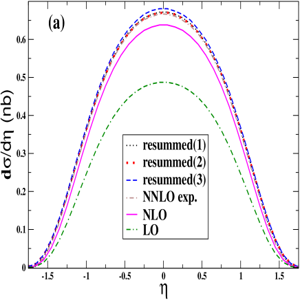
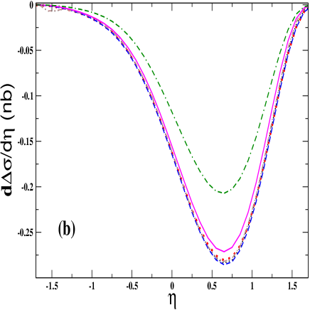
\psfrag{B}{(c)}\includegraphics[width=227.62204pt,height=170.71652pt,clip]{asymnew.eps}

Figure 1: (a) Differential cross section for $W^{+}$-production in unpolarized $pp$ collision at RHIC for ${\sqrt{S}}=500$ GeV as a function of the rapidity of the produced boson. (b) Same, but when one of the proton beams is longitudinally polarized. (c) The corresponding single-spin asymmetry ${\mathrm{A}}_{L}$. For all three plots, “resummed(1)” denotes the threshold-resummed cross section without including subleading $\ln(\bar{N})/N$ terms and without the $\cos\left(M\ln\frac{1}{\sqrt{z}}\right)$ term, while for “resummed(2)” the Cosine term is included. “Resummed(3)” is with the $\ln(\bar{N})/N$ terms. The curve labelled “NNLO exp.” gives the NNLO expansion of the “resummed(1)” result. We also display the LO and NLO cross sections.

Figures 1 (a) and (b) show the unpolarized and single-spin polarized cross sections for $W^{+}$-boson production in $\sqrt{S}=500$ GeV collisions at RHIC, as functions of the rapidity of the boson. We show the results at various levels of perturbation theory. The lower line in Fig. 1 (a) displays the unpolarized cross section at LO. The solid line above is the NLO result. The lines referred to as “resummed (1)-(3)” are for the matched NLL resummed cross section. As one can see, they all lie a few per cent higher than the NLO cross section. For the two dotted lines, denoted as “resummed (1)” and “resummed (2)”, the subleading pieces $\propto\ln(\bar{N})/N$ have been neglected. For “resummed (2)” the $\cos\left(M\ln\frac{1}{\sqrt{z}}\right)$ term discussed after Eq. (16) is kept in the Mellin moment integrand, whereas for “resummed (1)” it is ignored. This evidently leads to a negligible difference. The curve for “resummed (3)” then shows the effect of also including the subleading terms $\propto\ln(\bar{N})/N$. This leads to a further small increase of the predicted cross section. Finally, the remaining line, “NNLO exp.”, represents the two-loop (NNLO) expansion of the “resummed (1)” result. It shows that the NNLO terms generated by resummation are still significant, but that orders beyond NNLO have a negligible effect. We note that we have checked that the NLO expansion of the resummed cross section reproduces the exact NLO cross section very precisely. This provides confidence that the logarithmic terms that are subject to resummation indeed dominate the cross section, so that it is sensible to resum them. We use the same line coding for the polarized cross section in Fig. 1 (b).

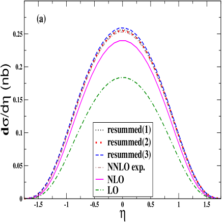
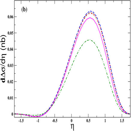
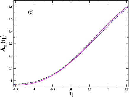
Figure 2: Same as Fig. 1, but for $W^{-}$ production.

Overall, we find rather moderate resummation effects at $\sqrt{S}=500$ GeV. In particular, resummation does not affect the rapidity dependence of the cross section much, in the sense that the shapes of the curves from NLO to the NLL resummed case are very similar. This was to be anticipated from our analytical results in Sec. III, where we found that the resummation of the rapidity-dependent cross section closely follows that of the rapidity-integrated one (see also LaenenSterman ). Figure 1 (c) shows the corresponding single-spin asymmetry, obtained by dividing the results in (a) and (b). The higher-order effects cancel almost entirely, and resummation becomes unimportant.

In Fig. 2 we display the corresponding results for $W^{-}$ production. Very similar quantitative features are found, except of course that the cross sections are smaller and, in the polarized case, of opposite sign because of the different combinations of parton distributions involved.

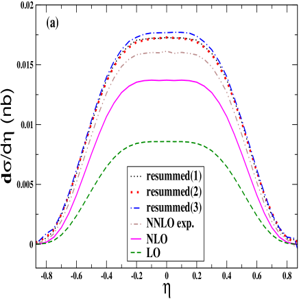
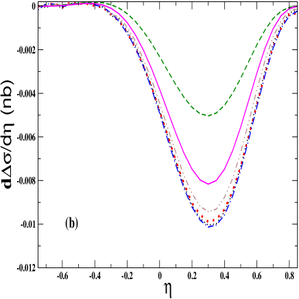
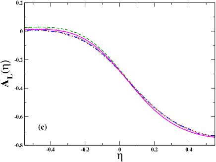
Figure 3: Same as Fig. 1, but for $\sqrt{S}=200$ GeV.

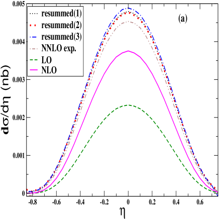
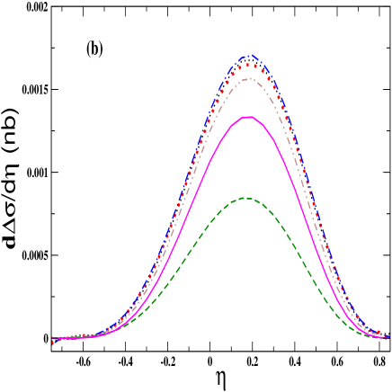
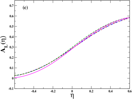
Figure 4: Same as Fig. 2, but for $\sqrt{S}=200$ GeV.

Threshold resummation should become more important when $\tau$ increases. We thus expect larger perturbative corrections at RHIC’s lower center-of-mass energy of $\sqrt{S}=200$ GeV. In Figs. 3 and 4 we repeat our calculations in Figs. 1 and 2 at this energy. Indeed, the resummation effects are much more significant, amounting to about 25% at mid rapidity. Also, since we are closer to threshold now, subleading $\ln(\bar{N})/N$ terms are less important than before. Of course, the cross sections are much smaller at $\sqrt{S}=200$ GeV than at 500 GeV. In fact, luminosity will need to be at least around the design luminosity of $320$/pb in order to have sufficient statistics for a good measurement. It was shown recently NadYuan2 that at this luminosity a statistical accuracy of 5% (9%) for the unpolarized $W^{+}$ ($W^{-}$) cross sections should be achievable, and that the current theoretical uncertainty related to the parton distributions is much larger, about 25%. It may therefore be quite possible to constrain better even the unpolarized parton distributions at large $x$ from measurements of $W^{\pm}$ production at RHIC at $\sqrt{S}=200$ GeV. Clearly, it will be crucial then to take into account the perturbative corrections we show in Figs. 3 and 4, since these are of similar size as the current parton distribution uncertainties.

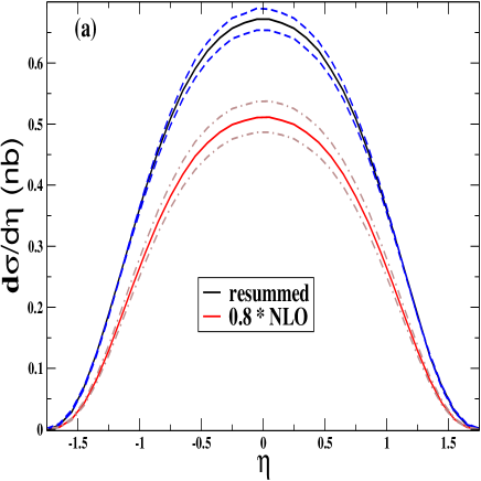
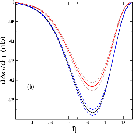
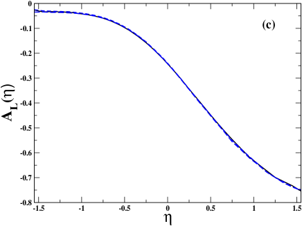
Figure 5: (a) Scale dependence of the NLO and the “resummed(1)” differential cross sections for $W^{+}$ production in unpolarized $pp$ collisions at RHIC at ${\sqrt{S}}=500$ GeV. We have varied the factorization/renormalization scale $\mu$ between $M_{W}/2$ and $2M_{W}$. Note that we have multiplied the NLO cross section by 0.8 for better visibility. The uppermost curves in each case are for the scale $M_{W}/2$. (b) Same for the singly-polarized cross section. (c) Scale dependence of the single-spin asymmetry ${\mathrm{A}}_{L}$, calculated from the resummed cross sections.

So far, we have always chosen the factorization and renormalization scales as $\mu=M_{W}$. As we discussed in Sec. IV, threshold resummation is expected to lead to a decrease of the scale dependence of the cross sections. We finally examine this in Fig. 5, where we vary the scales to $M_{W}/2$ and $2M_{W}$ in the NLO and the NLL “resummed(1)” cross sections for $W^{+}$ production at $\sqrt{S}=500$ GeV. Note that we have multiplied the NLO cross section by 0.8 for better visibility. As expected, the scale dependence is improved after resummation. At NLL, it becomes very small, and it cancels almost entirely in the spin asymmetry.

VII Conclusions and outlook

We have performed a study of perturbative higher-order corrections for $W^{\pm}$ production in singly-polarized $pp$ collisions at RHIC. This process will be used at RHIC to learn about the spin-dependent $u$ and $d$ distributions of the proton, and about the corresponding anti-quark distributions. In this work we have dealt with the resummation of potentially large “threshold” logarithms that arise when the incoming partons have just sufficient energy to produce the $W$ boson. We have performed the resummation to next-to-leading logarithmic accuracy. We have considered the resummation for the rapidity dependence of the cross sections, for which we have used a method developed in sv . We find that the resummation effect on the unpolarized and single-longitudinally polarized cross sections is rather moderate at RHIC’s higher energy $\sqrt{S}=500$ GeV, but more significant at $\sqrt{S}=200$ GeV where one is closer to threshold. The shapes of the $W$ rapidity distributions are rather unaffected by resummation. We believe that our study will be important in future extractions of the polarized, and even the unpolarized, $u,\bar{u},d,\bar{d}$ distributions from forthcoming RHIC data.

So far, we have only considered the $W^{\pm}$ as the observed final-state particles. Ultimately, for the comparison to future data, it will be necessary to extend our study to a calculation of the cross section for a single charged lepton, since this is the signal accessible at RHIC. This will be devoted to a later study. We believe, however, that the results presented here already give an excellent picture of the resummation effects to be expected when the $W$ decay is fully taken into account.

We finally note that the technique adopted in this work for treating the rapidity-dependence in the resummation for Drell-Yan type processes should also be useful for extending the recent study yokoya of the Drell-Yan process in $p\bar{p}$ collisions at the GSI to the rapidity-dependent case.

Appendix A

The NLO terms of the partonic coefficient functions in Eq. (4) read kubar ; weber ; tgdy ; smrs :

$$D_{q\bar{q}}^{(1)}\left(x_{1},x_{2},x_{1}^{0},x_{2}^{0},\frac{M_{W}^{2}}{\mu^{2}}\right) = C_{F}G^{A}(x_{1},x_{2},x_{1}^{0},x_{2}^{0})\,\Bigg{\{}\frac{2}{\left[(x_{1}-x_{1}^{0})(x_{2}-x_{2}^{0})\right]_{+}}+H^{A}(x_{1},x_{2},x_{1}^{0},x_{2}^{0})$$ (35)

$$\delta(x_{1}-x_{1}^{0})\,\delta(x_{2}-x_{2}^{0})\bigg{[}\pi^{2}-8+\ln^{2}\frac{(1-x_{1}^{0})(1-x_{2}^{0})}{x_{1}^{0}x_{2}^{0}}\bigg{]}$$

$$+\Bigg{(}\delta(x_{1}-x_{1}^{0})\bigg{[}\frac{2(x_{2}-x_{2}^{0})}{x_{2}^{2}+x_{2}^{0}\,{}^{2}}+\frac{2}{x_{2}-x_{2}^{0}}\ln\frac{2x_{2}^{0}}{x_{2}+x_{2}^{0}}$$

$$\hskip 17.07182pt+2\left(\frac{\ln(x_{2}-x_{2}^{0})}{x_{2}-x_{2}^{0}}\right)_{+}+\frac{2}{\left(x_{2}-x_{2}^{0}\right)_{+}}\ln\frac{1-x_{1}^{0}}{x_{1}^{0}x_{2}^{0}}\bigg{]}+(1\leftrightarrow 2)\Bigg{)}$$

$$+\ln\frac{M_{W}^{2}}{\mu^{2}}\Bigg{\{}\delta(x_{1}-x_{1}^{0})\,\delta(x_{2}-x_{2}^{0})\bigg{[}3+2\ln\frac{(1-x_{1}^{0})(1-x_{2}^{0})}{x_{1}^{0}x_{2}^{0}}\bigg{]}$$

$$\hskip 17.07182pt+\bigg{(}\delta(x_{1}-x_{1}^{0})\frac{2}{\left(x_{2}-x_{2}^{0}\right)_{+}}+(1\leftrightarrow 2)\bigg{)}\Bigg{\}}\Bigg{\}}\;,$$

$$D_{gq}^{(1)}\left(x_{1},x_{2},x_{1}^{0},x_{2}^{0},\frac{M_{W}^{2}}{\mu^{2}}\right) = T_{F}\Bigg{\{}\frac{\delta(x_{2}-x_{2}^{0})}{x_{1}^{3}}\Bigg{[}(x_{1}^{0}\,{}^{2}+(x_{1}-x_{1}^{0})^{2})\ln\frac{2(x_{1}-x_{1}^{0})(1-x_{2}^{0})}{(x_{1}+x_{1}^{0})x_{2}^{0}}$$ (36)

$$\hskip 17.07182pt+2x_{1}^{0}(x_{1}-x_{1}^{0})\Bigg{]}+\frac{G^{C}(x_{1},x_{2},x_{1}^{0},x_{2}^{0})}{(x_{2}-x_{2}^{0})_{+}}+H^{C}(x_{1},x_{2},x_{1}^{0},x_{2}^{0})$$

$$+\ln\frac{M_{W}^{2}}{\mu^{2}}\Bigg{\{}\frac{\delta(x_{2}-x_{2}^{0})}{x_{1}^{3}}(x_{1}^{0}\,{}^{2}+(x_{1}-x_{1}^{0})^{2})\Bigg{\}}\Bigg{\}}\;,$$

$$D_{qg}^{(1)}\left(x_{1},x_{2},x_{1}^{0},x_{2}^{0},\frac{M_{W}^{2}}{\mu^{2}}\right) = D_{gq}^{(1)}\left(x_{2},x_{1},x_{2}^{0},x_{1}^{0},\frac{M_{W}^{2}}{\mu^{2}}\right)\;,$$ (37)

$$\Delta D_{gq}^{(1)}\left(x_{1},x_{2},x_{1}^{0},x_{2}^{0},\frac{M_{W}^{2}}{\mu^{2}}\right) = T_{F}\Bigg{\{}\frac{\delta(x_{2}-x_{2}^{0})}{x_{1}^{2}}\Bigg{[}(2x_{1}^{0}-x_{1})\ln\frac{2(x_{1}-x_{1}^{0})(1-x_{2}^{0})}{(x_{1}+x_{1}^{0})x_{2}^{0}}$$ (38)

$$\hskip 17.07182pt+2(x_{1}-x_{1}^{0})\Bigg{]}+\frac{\Delta G^{C}(x_{1},x_{2},x_{1}^{0},x_{2}^{0})}{(x_{2}-x_{2}^{0})_{+}}+H^{C}(x_{1},x_{2},x_{1}^{0},x_{2}^{0})$$

$$+\ln\frac{M_{W}^{2}}{\mu^{2}}\Bigg{\{}\frac{\delta(x_{2}-x_{2}^{0})}{x_{1}^{2}}(2x_{1}^{0}-x_{1})\Bigg{\}}\Bigg{\}}\;,$$

$$\Delta D_{qg}^{(1)}\left(x_{1},x_{2},x_{1}^{0},x_{2}^{0},\frac{M_{W}^{2}}{\mu^{2}}\right) = \Delta D_{gq}^{(1)}\left(x_{2},x_{1},x_{2}^{0},x_{1}^{0},\frac{M_{W}^{2}}{\mu^{2}}\right)\;,$$ (39)

where

$$G^{A}(x_{1},x_{2},x_{1}^{0},x_{2}^{0}) = \frac{(x_{1}x_{2}+x_{1}^{0}x_{2}^{0})(x_{1}^{0}\,{}^{2}x_{2}^{0}\,{}^{2}+x_{1}^{2}x_{2}^{2})}{x_{1}^{2}x_{2}^{2}(x_{1}+x_{1}^{0})(x_{2}+x_{2}^{0})}\;,$$

$$H^{A}(x_{1},x_{2},x_{1}^{0},x_{2}^{0}) = -\frac{4x_{1}x_{2}x_{1}^{0}x_{2}^{0}(x_{1}+x_{1}^{0})(x_{2}+x_{2}^{0})}{(x_{1}^{0}x_{2}+x_{1}x_{2}^{0})^{2}\left(x_{1}^{2}x_{2}^{2}+x_{1}^{0}\,{}^{2}x_{2}^{0}\,{}^{2}\right)}\;,$$

$$G^{C}(x_{1},x_{2},x_{1}^{0},x_{2}^{0}) = \frac{2x_{2}^{0}(x_{1}^{0}\,{}^{2}x_{2}^{0}\,{}^{2}+(x_{1}^{0}x_{2}^{0}-x_{1}x_{2})^{2})(x_{1}^{0}x_{2}^{0}+x_{1}x_{2})}{x_{1}^{3}x_{2}^{2}(x_{1}x_{2}^{0}+x_{2}x_{1}^{0})(x_{2}+x_{2}^{0})}\;,$$

$$H^{C}(x_{1},x_{2},x_{1}^{0},x_{2}^{0}) = \frac{2x_{1}^{0}x_{2}^{0}(x_{1}^{0}x_{2}^{0}+x_{1}x_{2})(x_{1}x_{1}^{0}x_{2}^{2}+x_{1}^{0}x_{2}^{0}(x_{1}x_{2}^{0}+2x_{1}^{0}x_{2}))}{x_{1}^{2}x_{2}^{2}(x_{1}x_{2}^{0}+x_{2}x_{1}^{0})^{3}}\;,$$

$$\Delta G^{C}(x_{1},x_{2},x_{1}^{0},x_{2}^{0}) = \frac{2x_{2}^{0}(2x_{1}^{0}x_{2}^{0}-x_{1}x_{2})(x_{1}^{0}x_{2}^{0}+x_{1}x_{2})}{x_{1}^{2}x_{2}(x_{1}x_{2}^{0}+x_{2}x_{1}^{0})(x_{2}+x_{2}^{0})}\;.$$ (40)

Here the “plus”-distributions are defined as

$$\int_{x_{1}^{0}}^{1}dx_{1}\frac{f(x_{1})}{(x_{1}-x_{1}^{0})_{+}}\equiv\int_{x_{1}^{0}}^{1}dx_{1}\frac{f(x_{1})-f(x_{1}^{0})}{x_{1}-x_{1}^{0}}$$ (41)

(and likewise for $x_{2}$), and

$$\int_{x_{1}^{0}}^{1}dx_{1}\int_{x_{2}^{0}}^{1}dx_{2}\frac{g(x_{1},x_{2})}{\left[(x_{1}-x_{1}^{0})(x_{2}-x_{2}^{0})\right]_{+}}$$ (42)

$$\equiv \int_{x_{1}^{0}}^{1}dx_{1}\int_{x_{2}^{0}}^{1}dx_{2}\frac{g(x_{1},x_{2})-g(x_{1}^{0},x_{2})-g(x_{1},x_{2}^{0})+g(x_{1}^{0},x_{2}^{0})}{(x_{1}-x_{1}^{0})(x_{2}-x_{2}^{0})}\;.$$

References

• (1) for a recent review, see: S. D. Bass, arXiv:hep-ph/0411005.
• (2) for a review, see: G. Bunce, N. Saito, J. Soffer and W. Vogelsang, Ann. Rev. Nucl. Part. Sci.  50, 525 (2000) [arXiv:hep-ph/0007218]; C. Aidala et al., Research Plan for Spin Physics at RHIC, http://spin.riken.bnl.gov/rsc/report/masterspin.pdf
• (3) M. Wakamatsu and T. Watabe, Phys. Rev. D 62, 017506 (2000) [arXiv:hep-ph/9908425]; B. Dressler, K. Goeke, M. V. Polyakov and C. Weiss, Eur. Phys. J. C 14, 147 (2000) [arXiv:hep-ph/9909541]; Eur. Phys. C18, 719 (2001) [arXiv:hep-ph/9910464]; M. Glück and E. Reya, Mod. Phys. Lett. A 15, 883 (2000) [arXiv:hep-ph/0002182]; F. G. Cao and A. I. Signal, Phys. Rev. D 68, 074002 (2003) [arXiv:hep-ph/0306033]; M. Wakamatsu, Phys. Rev. D 67, 034005 (2003); Phys. Rev. D 67, 034006 (2003) [arXiv:hep-ph/0212356].
• (4) P. Amaudruz et al. [NMC], Phys. Rev. Lett. 66, 2712 (1991); M. Arneodo et al. [EMC], Phys. Rev. D 50, R1 (1994).
• (5) A. Baldit et al. [NA51 Collab.], Phys. Lett. 332, 244 (1994); E. A. Hawker et al. [FNAL E866/NuSea Collaboration], Phys. Rev. Lett.  80, 3715 (1998) [arXiv:hep-ex/9803011].
• (6) K. Ackerstaff et al. [HERMES Collab.], Phys. Rev. Lett.  81, 5519 (1998) [arXiv:hep-ex/9807013].
• (7) B. Adeva et al. [Spin Muon Collaboration], Phys. Lett. B 420, 180 (1998) [arXiv:hep-ex/9711008].
• (8) A. Airapetian et al. [HERMES Collaboration], Phys. Rev. Lett.  92, 012005 (2004) [arXiv:hep-ex/0307064]; Phys. Rev. D 71, 012003 (2005) [arXiv:hep-ex/0407032].
• (9) S. Platchkov [COMPASS Collaboration], talk given at the “Particles and Nuclei International Conference (PANIC05)”, Santa Fe, New Mexico, October 2005.
• (10) X. d. Jiang, talk given at the “1st Workshop on Quark-Hadron Duality and the Transition to pQCD”, Frascati, Rome, Italy, June 2005, arXiv:hep-ex/0510011.
• (11) M. Stratmann and W. Vogelsang, Phys. Rev. D 64, 114007 (2001) [arXiv:hep-ph/0107064]; M. Glück, E. Reya, arXiv:hep-ph/0203063; A. Kotzinian, Phys. Lett. B 552, 172 (2003) [arXiv:hep-ph/0211162]; Eur. Phys. J. C 44, 211 (2005) [arXiv:hep-ph/0410093]; G. A. Navarro and R. Sassot, Eur. Phys. J. C 28, 321 (2003) [arXiv:hep-ph/0302053]; E. Christova, S. Kretzer, E. Leader, Eur. Phys. J. C 22, 269 (2001) [arXiv:hep-ph/0108055]; E. Leader and D. B. Stamenov, Phys. Rev. D 67, 037503 (2003) [arXiv:hep-ph/0211083]; S. D. Bass, Phys. Rev. D 67, 097502 (2003) [arXiv:hep-ph/0210214].
• (12) C. Bourrely and J. Soffer, Phys. Lett. B 314, 132 (1993); Nucl. Phys. B 423, 329 (1994) [arXiv:hep-ph/9405250]; Nucl. Phys. B 445, 341 (1995) [arXiv:hep-ph/9502261]; P. Chiappetta and J. Soffer, Phys. Lett. B 152, 126 (1985).
• (13) N. S. Craigie, K. Hidaka, M. Jacob and F. M. Renard, Phys. Rept.  99, 69 (1983); C. Bourrely, J. Soffer and E. Leader, Phys. Rept.  59, 95 (1980).
• (14) L. C. Bland [STAR Collaboration], talk presented at the “Circum-Pan-Pacific RIKEN Symp. High Energy Spin Phys. (Pacific Spin 99)”, RIKEN Rev.  28, 8 (2000) [arXiv:hep-ex/0002061].
• (15) P. M. Nadolsky and C. P. Yuan, Nucl. Phys. B 666, 31 (2003) [arXiv:hep-ph/0304002]
• (16) P. M. Nadolsky and C. P. Yuan, Nucl. Phys. B 666, 3 (2003) [arXiv:hep-ph/0304001].
• (17) P.M. Nadolsky, talk presented at the workshop “Spin & $pp$ Physics at RHIC II”, Brookhaven National Laboratory, Upton, New York, October 2005.
• (18) G. Altarelli, R. K. Ellis and G. Martinelli, Nucl. Phys. B 157, 461 (1979).
• (19) J. Kubar, M. Le Bellac, J. L. Meunier and G. Plaut, Nucl. Phys. B 175, 251 (1980).
• (20) P. Ratcliffe, Nucl. Phys. B 223, 45 (1983).
• (21) A. Weber, Nucl. Phys. B 382, 63 (1992).
• (22) A. Weber, Nucl. Phys. B 403, 545 (1993).
• (23) B. Kamal, Phys. Rev. D 53, 1142 (1996) [arXiv:hep-ph/9511217]; ibid. 57, 6663 (1998) [arXiv:hep-ph/9710374].
• (24) T. Gehrmann, Nucl. Phys. B 498, 245 (1997) [arXiv:hep-ph/9702263].
• (25) T. Gehrmann, Nucl. Phys. B 534, 21 (1998) [arXiv:hep-ph/9710508].
• (26) M. Glück, A. Hartl and E. Reya, Eur. Phys. J. C 19, 77 (2001) [arXiv:hep-ph/0011300].
• (27) G. Sterman, Nucl. Phys. B 281, 310 (1987).
• (28) S. Catani and L. Trentadue, Nucl. Phys. B 327, 323 (1989); Nucl. Phys. B 353, 183 (1991).
• (29) for a review see, for example: N. Kidonakis, Int. J. Mod. Phys. A 15, 1245 (2000) [arXiv:hep-ph/9902484]. For work that rederives some of the earlier results in different context, see: S. Forte and G. Ridolfi, Nucl. Phys. B 650, 229 (2003) [arXiv:hep-ph/0209154]; A. V. Manohar, Phys. Rev. D 68, 114019 (2003) [arXiv:hep-ph/0309176]; A. Idilbi and X. d. Ji, Phys. Rev. D 72, 054016 (2005) [arXiv:hep-ph/0501006].
• (30) see: S. Moch and A. Vogt, Phys. Lett. B 631, 48 (2005) [arXiv:hep-ph/0508265]; E. Laenen and L. Magnea, Phys. Lett. B 632, 270 (2006) [arXiv:hep-ph/0508284]; A. Idilbi, X. d. Ji, J. P. Ma and F. Yuan, arXiv:hep-ph/0509294; V. Ravindran, arXiv:hep-ph/0512249. These papers even contain many of the ingredients needed to perform the resummation to complete N3LL accuracy.
• (31) G. Sterman and W. Vogelsang, JHEP 0102, 016 (2001) [arXiv:hep-ph/0011289].
• (32) E. Laenen and G. Sterman, FERMILAB-CONF-92-359-T Presented at Particles & Fields 92: 7th Meeting of the Division of Particles Fields of the APS (DPF 92), Batavia, IL, 10-14 Nov 1992.
• (33) E. Laenen, G. Sterman and W. Vogelsang, Phys. Rev. Lett.  84, 4296 (2000) [arXiv:hep-ph/0002078]; Phys. Rev. D 63, 114018 (2001) [arXiv:hep-ph/0010080].
• (34) T. O. Eynck, E. Laenen and L. Magnea, JHEP 0306, 057 (2003) [arXiv:hep-ph/0305179].
• (35) J. Kodaira and L. Trentadue, Phys. Lett. B 112, 66 (1982); Phys. Lett. B 123, 335 (1983);
S. Catani, E. D’Emilio and L. Trentadue, Phys. Lett. B 211, 335 (1988).
• (36) S. Catani, M. L. Mangano, P. Nason and L. Trentadue, Nucl. Phys. B 478, 273 (1996) [arXiv:hep-ph/9604351].
• (37) S. Catani, M. L. Mangano and P. Nason, JHEP 9807, 024 (1998) [arXiv:hep-ph/9806484].
• (38) S. Catani, D. de Florian and M. Grazzini, in: W. Giele et al., arXiv:hep-ph/0204316;
S. Catani, D. de Florian and M. Grazzini, JHEP 0201, 015 (2002) [arXiv:hep-ph/0111164].
• (39) A. Kulesza, G. Sterman and W. Vogelsang, Phys. Rev. D 66, 014011 (2002) [arXiv:hep-ph/0202251]; Phys. Rev. D 69, 014012 (2004) [arXiv:hep-ph/0309264].
• (40) X. Chen, Y. Mao and B. Q. Ma, Nucl. Phys. A 759, 188 (2005) [arXiv:hep-ph/0505127].
• (41) M. Glück, E. Reya, M. Stratmann and W. Vogelsang, Phys. Rev. D 63, 094005 (2001) [arXiv:hep-ph/0011215].
• (42) M. Glück, E. Reya, and A. Vogt, Eur. Phys. J. C5, 461 (1998) [arXiv:hep-ph/9806404].
• (43) H. Shimizu, G. Sterman, W. Vogelsang and H. Yokoya, Phys. Rev. D 71, 114007 (2005) [arXiv:hep-ph/0503270].
• (44) P. J. Sutton, A. D. Martin, R. G. Roberts and W. J. Stirling, Phys. Rev. D 45, 2349 (1992).