On the Observation of Vacuum Birefringence

Abstract

We suggest an experiment to observe vacuum birefringence induced by intense laser fields. A high-intensity laser pulse is focused to ultra-relativistic intensity and polarizes the vacuum which then acts like a birefringent medium. The latter is probed by a linearly polarized x-ray pulse. We calculate the resulting ellipticity signal within strong-field QED assuming Gaussian beams. The laser technology required for detecting the signal will be available within the next three years.

The interactions of light and matter are described by quantum electrodynamics (QED), at present the best-established theory in physics. The QED Lagrangian couples photons to charged Dirac particles in a gauge invariant way. At photon energies small compared to the electron mass, $\omega\ll m_{e}$, electrons (and positrons) will generically not be produced as real particles. Nevertheless, as already stated by Heisenberg and Euler, “…even in situations where the [photon] energy is not sufficient for matter production, its virtual possibility will result in a ‘polarization of the vacuum’ and hence in an alteration of Maxwell’s equations” heisenberg:1936 . These authors were the first to explicitly derive the nonlinear terms induced by QED for small photon energies but arbitrary intensities (see also weisskopf:1936 ).

The most spectacular process resulting from these modifications presumably is pair production in a constant electric field. This is an absorptive process as photons disappear by disintegration into matter pairs. It can occur for field strengths larger than the critical one given by sauter:1931 ; schwinger:1951

$$E_{c}\equiv\frac{m_{e}^{2}}{e}\simeq 1.3\times 10^{18}\,\mathrm{V/m}\;.$$ (1)

In this electric field an electron gains an energy $m_{e}$ upon travelling a distance equal to its Compton wavelength, ${\mathchoice{\hbox{\raise 5.06941pt\hbox to0.0pt{\kern 1.16664pt\vrule width=4.08333pt,height=0.1pt,depth=0.1pt\hss}\hbox{$\displaystyle\lambda$}}}{\hbox{\raise 5.06941pt\hbox to0.0pt{\kern 1.16664pt\vrule width=4.08333pt,height=0.1pt,depth=0.1pt\hss}\hbox{$\textstyle\lambda$}}}{\hbox{\raise 3.54857pt\hbox to0.0pt{\kern 0.81665pt\vrule width=2.85832pt,height=0.1pt,depth=0.1pt\hss}\hbox{$\scriptstyle\lambda$}}}{\hbox{\raise 2.5347pt\hbox to0.0pt{\kern 0.58331pt\vrule width=2.04166pt,height=0.1pt,depth=0.1pt\hss}\hbox{$\scriptscriptstyle\lambda$}}}}_{e}=1/m_{e}$. The associated intensity is $I_{c}=E_{c}^{2}\simeq 4.4\times 10^{29}$ W/cm² such that both field strength and intensity are way out of experimental reach for the time being – unless one can utilize huge relativistic gamma factors produced by large scale particle accelerators bula:1996 ; burke:1997 .

Alternatively, there are also dispersive effects that may be considered. These include many of the phenomena studied in nonlinear optics as well as “birefringence of the vacuum” first addressed by Klein and Nigam klein:1964 in 1964, soon followed by more systematic studies BB:1967 ; bialynicka-birula:1970 ; brezin:1970b . In essence, the polarized QED vacuum acts like a birefringent medium (e.g. a calcite crystal) with two indices of refraction depending on the polarization of the incoming light. In a static magnetic field of $5\,\mathrm{T}$ a light polarization rotation has recently been observed zavattini:2005 . The measured signal differs from the QED expectations and may be caused by a new coupling of photons to an hitherto unobserved pseudoscalar.

Detection of the tiny dispersive effects is an enormous challenge. In this paper we point out that several orders of magnitude in field strength may be gained by employing high-power lasers. Distorting the vacuum with lasers has been suggested long ago brezin:1970b but was not considered experimentally for lack of sufficient laser power. However, recent progress in both laser technology and x-ray detection has lead to novel experimental capabilities. It is therefore due time to specifically address the feasibility of a strong-field laser experiment to measure vacuum birefringence. In the light of the results zavattini:2005 such experiments are also necessary in order to test whether strong electromagnetic fields provide windows into new physics.

We intend to utilize the high-repetition rate petawatt class laser system POLARIS which is currently under construction at the Jena high-intensity laser facility and which will be fully operational in 2007 hein:2004 . POLARIS consists of a diode-pumped laser system based on chirped pulse amplification (CPA) which will be operating at $\Lambda=1032\,\mathrm{nm}$ ($\Omega=1.2$ eV) with a repetition rate of $0.1\,\mathrm{Hz}$. A pulse duration of about $140\,\mathrm{fs}$ and a pulse energy of $150\,\mathrm{J}$ in principle allows to generate intensities in the focal region of $I=10^{22}\,\mathrm{W/cm^{2}}$. This corresponds to a substantial electric field $E\simeq 2\times 10^{14}\,\mathrm{V/m}$, still about four orders of magnitude below $E_{c}$.

The proposed experimental setup is shown in Fig. 1. A high-intensity laser pulse is focused by an off-axis parabolic mirror. A linearly polarized laser-generated ultra-short x-ray pulse is aligned collinearly with the focused optical laser pulse. After passing through the focus the laser induced vacuum birefringence will lead to a small ellipticity of the x-ray pulse which will be detected by a high contrast x-ray polarimeter hart:1991 . The whole setup is located in an ultra-high vacuum chamber and is entirely computer controlled.

Shown in grey in Fig. 1 is an extension of the setup which enables us to accurately overlap two counter propagating high-intensity laser pulses. Accurate control over spatial and temporal overlap was convincingly demonstrated carrying out an autocorrelation of the laser pulses at full intensity liesfeld:2005 and generating Thomson backscattered x-rays from laser-accelerated electrons schwoerer:2005 . This counter propagating scheme, a table-top “photon collider”, may also be employed for pair creation from the vacuum. For the x-ray probe pulse we have chosen an x-ray source of photon energy $\omega\simeq 1$ keV, since the birefringence signal is proportional to $\omega^{2}$ (see below) . Our long-term plans are to replace the present source by an x-ray free electron laser (XFEL) or by a laser-based Thomson backscattering source schwoerer:2005 both of which deliver ultrashort and highly polarized x-rays.

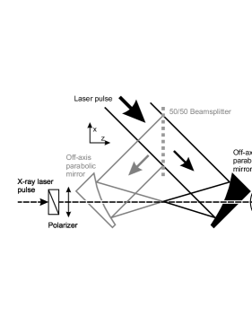
Figure 1: Proposed experimental setup for the demonstration of vacuum birefringence: A high-intensity laser pulse is focused by an $F/2.5$ off-axis parabolic mirror. A hole is drilled into the parabolic mirror in alignment with the $z$-axis (axes as indicated) in such a way that an x-ray pulse can propagate along the $z$-axis through the focal region of the high-intensity laser pulse. Using a polarizer-analyzer pair the ellipticity of the x-ray pulse may be detected. Shown in grey: Extension of the setup for the generation of counter propagating laser pulses and a high-intensity standing wave which may be used for pair creation.

Refraction is a dispersive process based on modified propagation properties of the probe photons travelling through a region where a (strong) background field is present. The resulting corrections to pure Maxwell theory to leading order in the probe field $a_{\mu}$ may be expressed in terms of an effective action brezin:1970b

$$\delta S\equiv{\textstyle\frac{1}{2}}\int d^{4}x\,d^{4}y\,a_{\mu}(x)\Pi^{\mu\nu}(x,y;A)a_{\nu}(y)\;,$$ (2)

where $A_{\mu}$ denotes the background field and $\Pi^{\mu\nu}$ the polarization tensor. To lowest order in a loop (or $\hbar$) expansion the former is given by the Feynman diagram

(3)

with the heavy lines denoting the dressed propagator depending on the background field $A$,

(4)

Hence, $S_{F}[A]$ is an infinite series of diagrams where the $n$th term corresponds to the absorption and/or emission of $n-1$ background photons (represented by the dashed external lines) by the “bare” electron.

The dressed propagator is known exactly only for a few special background configurations (see dittrich:2000 for an overview). Typically, one obtains rather unwieldy integral representations which have to be analyzed numerically. In our case, however, we can exploit the fact that we are working in the regime of both low energy and small intensities leading to two small parameters affleck:1987 , namely

$$\nu^{2} \equiv \omega^{2}/m_{e}^{2}\simeq 4\times 10^{-6}\;,$$ (5)

$$\epsilon^{2} \equiv E^{2}/E_{c}^{2}=I/I_{c}\simeq 2\times 10^{-8}\;.$$ (6)

Low intensity, $\epsilon^{2}\ll 1$, means that we can work to lowest nontrivial order in the external field i.e. $O(\epsilon^{2})$. In terms of Feynman diagrams (3) then reduces to

(7)

Low energy, $\nu\ll 1$, implies that we may safely expand $\Pi^{\mu\nu}$ in derivatives or, after Fourier transformation, in powers of the probe 4-momentum $k=\omega(1,n\mbox{\bf k})$ where $\mbox{\bf k}^{2}=1$ and $n\geq 1$ is the index of refraction. Thus, the derivative expansion is in powers of $\omega^{2}$ or, equivalently, of $\nu^{2}$. Again we restrict our analysis to leading order which turns out to be $\nu^{2}$. The first vacuum polarization diagram in (7) is $O(\nu^{4})$ while the second is $O(\epsilon^{2}\nu^{2})$ so we may safely neglect the former. The low-energy limit of the remaining diagram is obtained from the celebrated Heisenberg-Euler Lagrangian heisenberg:1936 which to leading order in $\epsilon^{2}$ is given by

$$\delta\mathscr{L}(\mathscr{S},\mathscr{P})={\textstyle\frac{1}{2}}\gamma_{-}\mathscr{S}^{2}+{\textstyle\frac{1}{2}}\gamma_{+}\mathscr{P}^{2}\;.$$ (8)

The basic building blocks in (8) are the scalar and pseudoscalar invariants schwinger:1951 ; bialynicka-birula:1970

$$\mathscr{S} \equiv -{\textstyle\frac{1}{4}}F_{\mu\nu}F^{\mu\nu}={\textstyle\frac{1}{2}}(\mbox{\boldmath$E$}^{2}-\mbox{\boldmath$B$}^{2})\;,$$ (9)

$$\mathscr{P} \equiv -{\textstyle\frac{1}{4}}F_{\mu\nu}\tilde{F}^{\mu\nu}=\mbox{\boldmath$E$}\cdot\mbox{\boldmath$B$}\;,$$ (10)

where $F_{\mu\nu}$ denotes the electromagnetic field-strength tensor (comprising both background and probe photon field) and $\tilde{F}_{\mu\nu}$ its dual. The nonlinear couplings in (8) are given by

$$\gamma_{+}\equiv 7\rho\;,\quad\gamma_{-}\equiv 4\rho\;,\quad\rho\equiv\frac{\alpha}{45\pi}\frac{1}{E_{c}^{2}}\;,$$ (11)

with $\alpha=1/137$ being the fine-structure constant.

To proceed we split the fields into an intense (laser) background and a weak probe field according to the replacement $F_{\mu\nu}\to F_{\mu\nu}+f_{\mu\nu}$ with upper (lower) case letters for electromagnetic quantities henceforth referring to the background (probe). In the following we regard the plane wave probe field $f_{\mu\nu}$ as a weak disturbance on top of the strong background field $F_{\mu\nu}$ which we take as an electromagnetic wave of frequency $\Omega$. It can be a plane or standing wave or more realistic variants thereof like Gaussian beams (see discussion below). In any case, for the actual experiment we will have the hierarchy of frequencies $\Omega\ll\omega\ll m_{e}$ in agreement with (5).

The leading-order contribution to the polarization tensor is found by performing the split $F\to F+f$ in the Heisenberg-Euler action, $\delta S=\int d^{4}x\,\delta\mathscr{L}$, and writing it in the form (2). This yields a polarization tensor

$$\Pi^{\mu\nu}=-\gamma_{-}\,k^{2}\mathscr{S}\,\mathbb{P}^{\mu\nu}+\gamma_{-}\,b^{\mu}b^{\nu}+\gamma_{+}\,\tilde{b}^{\mu}\tilde{b}^{\nu}\;,$$ (12)

where $\mathbb{P}^{\mu\nu}=g^{\mu\nu}-k^{\mu}k^{\nu}/k^{2}$ is the standard projection orthogonal to $k$ and $\mathscr{S}$ denotes the background invariant. In addition we have introduced the new 4-vectors bialynicka-birula:1970 ,

$$b^{\mu}\equiv F^{\mu\nu}k_{\nu}\;,\quad\tilde{b}^{\mu}\equiv\tilde{F}^{\mu\nu}k_{\nu}\;.$$ (13)

Note that we have $b\cdot k=0=\tilde{b}\cdot k$ and hence $\Pi^{\mu\nu}k_{\nu}=0$ as required by gauge invariance. It is useful to diagonalize $\Pi^{\mu\nu}$ and rewrite it in terms of a spectral decomposition. In full generality this is a bit awkward, but for our purposes matters can be simplified. The eigenvalues of $\Pi^{\mu\nu}$ in principle depend on the four invariants $k^{2}$, $\mathscr{S}$, $\mathscr{P}$ and $b^{2}$. From (12) we note that there is no $\mathscr{P}$ dependence and that only the combination $k^{2}\mathscr{S}$ appears. Let us count powers of $\epsilon$ and $\nu$ to determine the relative magnitudes of the invariants. If we write the index of refraction as $n=1+\Delta$ we expect $\Delta=O(\epsilon^{2})$ the deviation of $n$ from unity being due to the external fields. Hence $k^{2}$ is no longer zero but rather $k^{2}=O(\epsilon^{2}\nu^{2})$ implying $k^{2}\mathscr{S}=O(\epsilon^{4}\nu^{2})$. For generic geometrical settings (see below) the invariant $b^{2}=O(\epsilon^{2}\nu^{2})$. The upshot of this power counting exercise is the important inequality

$$|k^{2}\mathscr{S}|\ll|b^{2}|\;,$$ (14)

by means of which we may neglect $k^{2}\mathscr{S}$. This justifies the statement in dittrich:2000 that to leading order in $\epsilon$ and $\nu$ the eigenvalues of $\Pi^{\mu\nu}$ do not depend on the invariants $\mathscr{S}$ and $\mathscr{P}$. Hence, under the assertion (14) constant fields behave as crossed fields ($E$ and $B$ orthogonal and of the same magnitude) for which strictly $\mathscr{S}=\mathscr{P}=0$. In addition, one has $b^{2}=\tilde{b}^{2}$ and $b\cdot\tilde{b}=0$ so that (12) turns into the spectral representation

$$\Pi^{\mu\nu}=\gamma_{-}\,b^{\mu}b^{\nu}+\gamma_{+}\,\tilde{b}^{\mu}\tilde{b}^{\nu}\;.$$ (15)

We read off that the (nontrivial) eigenvectors are given by (13) corresponding to eigenvalues $\gamma_{\pm}b^{2}(k)$. Note that $b^{2}$ is the only nonvanishing invariant which can be built from crossed fields.

Adopting a plane wave ansatz for the probe field $a_{\mu}$ yields a homogeneous wave equation which in momentum space becomes linear algebraic. It has nontrivial solutions only if a secular equation holds which determines the dispersion relations for $k^{2}$. With the eigenvalues given above there are two of them, $k^{2}-\gamma_{\pm}b^{2}(k)=0$. Inserting $k=\omega(1,n\mbox{\bf k})$, we finally obtain two solutions for the index of refraction,

$$n_{\pm}=1+{\textstyle\frac{1}{2}}\gamma_{\pm}Q^{2}\;.$$ (16)

The nonnegative quantity $Q^{2}$ is an energy density which in 3-vector notation becomes

$$Q^{2}=\mbox{\boldmath$E$}^{2}+\mbox{\boldmath$B$}^{2}-2\mbox{\boldmath$S$}\cdot\mbox{\bf k}-(\mbox{\boldmath$E$}\cdot\mbox{\bf k})^{2}-(\mbox{\boldmath$B$}\cdot\mbox{\bf k})^{2}\;,$$ (17)

with $\mbox{\boldmath$S$}=\mbox{\boldmath$E$}\times\mbox{\boldmath$B$}$ being the Poynting vector. The inequality (14) holds as long as $Q^{2}\neq 0$. The indices of refraction become maximal if probe and background are counter propagating (‘head-on collision’), $\mbox{\bf k}=-\mbox{\boldmath$S$}/|\mbox{\boldmath$S$}|$, whereupon

$$Q^{2}=\mbox{\boldmath$E$}^{2}+\mbox{\boldmath$B$}^{2}+2|\mbox{\boldmath$S$}|\equiv 4I\;,$$ (18)

with $I$ denoting the background intensity. Note that one gains a factor of four as compared to a purely electric or purely magnetic background. Plugging (18) into (16) the indices of refraction become $n_{\pm}=1+2\gamma_{\pm}I$ or, upon inserting $\gamma_{\pm}$,

$$n_{\pm}=1+\left\{14\atop 8\right\}\rho I=1+\frac{\alpha}{45\pi}\left\{14\atop 8\right\}\frac{I}{I_{c}}\;.$$ (19)

To the best of our knowledge, these values have first been obtained in BB:1967 . They imply birefringence with a relative phase shift between the two rays proportional to $\triangle n\equiv n_{+}-n_{-}$,

$$\triangle\phi=2\pi\frac{d}{\lambda}\triangle n=\frac{4\alpha}{15}\frac{d}{\lambda}\frac{I}{I_{c}}=\frac{4\alpha}{15}\frac{d}{\lambda}\epsilon^{2}\;.$$ (20)

Table 1: Numerical values for the phase shift (21) and ellipticity signal $\delta^{2}$. First line: present specifications of the Jena laser facility. Second line: optimal scenario with XFEL probe and large Rayleigh length. The peak intensity is taken to be $I_{0}=10^{22}$ W/cm².

$\omega$ / keV	$\lambda$ / nm	$z_{0}$ / $\mu$m	$\triangle\phi$ / rad	$\delta^{2}$
1.0	1.2	10	$1.2\times 10^{-6}$	$3.4\times 10^{-13}$
15	0.08	25	$4.4\times 10^{-5}$	$4.8\times 10^{-10}$

A realistic laser field will lead to an intensity distribution along the $z$-axis (choosing $\mbox{\bf k}=\mbox{\boldmath$e$}_{z}$). If $z_{0}$ measures the typical extension of the distribution we may set $s\equiv z/z_{0}$ and write the intensity as $I(s)=I_{0}\,g(s)$ with peak intensity $I_{0}$ and a dimensionless distribution function $g(s)$. The phase shift (20) is then replaced by the expression koch:2004

$$\triangle\phi=\frac{4\alpha}{15}\frac{z_{0}}{\lambda}\frac{I_{0}}{I_{c}}\kappa\;,$$ (21)

where the correction factor $\kappa$ is the integral

$$\kappa=\kappa(s_{0})\equiv\int_{-s_{0}}^{s_{0}}ds\,g(s)=O(1)\;.$$ (22)

Here, $s_{0}$ denotes the half-width of the intensity distribution in units of $z_{0}$. In general it is a reasonable approximation to let $s_{0}\to\infty$. For a single Gaussian beam, $z_{0}$ is the Rayleigh length and the intensity $I_{1}$ follows a Lorentz curve, hence $g_{1}(s)=1/(1+s^{2})$ implying $\kappa_{1}(\infty)=\pi$. Identifying $d=2z_{0}$ this differs from (20) by a factor of $\pi/2=O(1)$. For two counter propagating Gaussian beams (‘standing wave’) obtained from splitting a beam of intensity $I_{1}$ one gains a factor of two in peak intensity but the distribution gets thinned out due to the usual $\cos^{2}$ modulation, which cancels the gain in intensity leading to the same correction factor $\kappa_{2}=\pi=\kappa_{1}$.

A linearly polarized electromagnetic wave undergoing vacuum birefringence with a polarization vector oriented under an angle of $45^{\circ}$ with respect to both background fields $E$ and $B$ will be rendered elliptically polarized with ellipticity $\delta$ (ratio of the field vectors). In the experiment, intensities will be measured and the experimental quantity to be determined is $\delta^{2}\simeq(\frac{1}{2}\Delta\phi)^{2}$. In Table 1 expected ellipticity values for given experimental parameters are listed.

These results clearly show the challenging nature but also the feasibility of the proposed experiment. Presently, a petawatt class laser facility such as POLARIS is expected to reach about $10^{22}\,\mathrm{W/cm^{2}}$ at unprecedented repetition rates of $\sim 0.1\,\mathrm{Hz}$ hein:2004 . The values of $\delta^{2}$ obtained for such lasers (Tab. 1) are at the limit of the accuracy that can now be obtained with high-contrast x-ray polarimeters using multiple Bragg reflections from channel-cut perfect crystals hart:1991 ; hasegawa:1999 ; alp:2000 . These instruments are in principle capable of a sensitivity of $\delta^{2}\simeq 10^{-11}$ alp:2000 . Since the expected signal is proportional to both $I^{2}$ and $\lambda^{-2}$ it may be greatly enhanced by increasing the laser intensity or choosing a smaller probe pulse wave length. For example, with the proposed ELI laser facility reaching $10^{25}\,\mathrm{W/cm^{2}}$ mourou:2005 a sensitivity of the polarimeter of only $10^{-7}\dots 10^{-4}$ is required which is within presently demonstrated values of sensitivity hart:1991 . The required x-ray probe pulse may be generated either with an XFEL synchronized to a petawatt laser or by the use of Thomson scattered laser photons from monochromatic laser accelerated electron beams schwoerer:2005 ; faure:2004 .

It seems worthwhile to point out that although a standing wave for the background (which may be created in the “photon collider” setup as shown in Fig. 1) does not lead to an increase in integrated intensity and hence of the birefringence signal, it does yield double peak intensity. This is important for the observation of effects sensitive to localized intensity like Cherenkov radiation and pair production.

This work was supported by the DFG Project TR 18. The authors gratefully acknowledge stimulating discussions with H. Gies, A. Khvedelidze, M. Lavelle, V. Malka, D. McMullan, G. Mourou, A. Nazarkin, A. Ringwald and O. Schröder.

References

- (1) W. Heisenberg and H. Euler, Z. Phys. 98, 714 (1936).
- (2) V. Weisskopf, K. Dan. Vidensk. Selsk. Mat. Fys. Medd., 14, 6 (1936), reprinted in Quantum Electrodynamics, J. Schwinger, ed., Dover, New York 1958.
- (3) F. Sauter, Z. Phys. 69, 742 (1931).
- (4) J. Schwinger, Phys. Rev. 82, 664 (1951).
- (5) C. Bula et al., Phys. Rev. Lett. 76, 3116 (1996).
- (6) D. Burke et al., Phys. Rev. Lett. 79, 1629 (1997).
- (7) J. Klein and B. Nigam, Phys. Rev. 135, B1279 (1964).
- (8) R. Baier and P. Breitenlohner, Acta Phys. Austriaca 25, 212 (1967); Nuovo Cim. B 47, 117 (1967).
- (9) Z. Białynicka-Birula and I. Białynicki-Birula, Phys. Rev. D2, 2341 (1970).
- (10) E. Brezin and C. Itzykson, Phys. Rev. D3, 618 (1970).
- (11) E. Zavattini et. al., PVLAS collaboration (2005), hep-ex/0507107.
- (12) J. Hein et al., Appl. Phys. B 79, 419 (2004).
- (13) M. Hart et al., Rev. Sci. Instrum. 62, 2540 (1991).
- (14) B. Liesfeld et al., Appl. Phys. Lett., 86, 161107 (2005).
- (15) H. Schwoerer et al., Phys. Rev. Lett. (2005), accepted for publication.
- (16) W. Dittrich and H. Gies, Probing the quantum vacuum, vol. 166 of Springer Tracts Mod. Phys. (Springer, Berlin, 2000).
- (17) I. Affleck and L. Kruglyak, Phys. Rev. Lett. 59, 1065 (1987).
- (18) K. Koch, diploma thesis, Jena (2004), in German.
- (19) Y. Hasegawa et al., Acta Cryst. A 55, 955 (1999).
- (20) E. Alp, W. Sturhahn, and T. Toellner, Hyperfine Interactions 125, 45 (2000).
- (21) G. Mourou and V. Malka, private communication (2005).
- (22) J. Faure et al., Nature 431 (7008), 541 (2004).