We show that the well-known divergence of the perturbative expansion of resummed results for processes such as deep-inelastic scattering and Drell-Yan in the soft limit can be treated by Borel resummation. The divergence in the Borel inversion can be removed by the inclusion of suitable higher twist terms. This provides us with an alternative to the standard ’minimal prescription’ for the asymptotic summation of the perturbative expansion, and it gives us some handle on the role of higher twist corrections in the soft resummation region.

December 2005

It has been known for some time [1] that the resummation of logarithmically enhanced contributions to the coefficients of the QCD perturbative expansion due to soft gluon radiation has the effect of rescaling the argument of the strong coupling constant: the hard perturbative scale is replaced by a relatively soft scale related to the radiation process. For example, for a physical process characterized by the hard scale $Q^{2}$ and a scaling variable $0\leq x\leq 1$ near the $x=1$ boundary of phase space (e.g. close to the production threshold for a given final state), the resummation of large logs of $1-x$ effectively replaces the perturbative coupling $\alpha_{s}(Q^{2})$ with $\alpha_{s}(Q^{2}(1-x))$. Similarly, in the resummation of soft $p_{T}$ spectra [2] the argument of the strong coupling becomes $p_{T}^{2}$, and so on. Therefore, the perturbative approach eventually fails in this ‘soft’ kinematical region. This failure is understandable on physical grounds, because at the phase space boundary, i.e. as $x\to 1$, the center–of–mass energy is just sufficient to produce the given final state, so, for instance in the case of deep-inelastic scattering in this limit the process becomes elastic.

In practice, this problem must be treated in some way in order to obtain phenomenological predictions: eventually, at some low scale $\Lambda$ (the position of the Landau pole) the strong coupling blows up, so when

$$x=x_{L}\equiv 1-\frac{\Lambda^{2}}{Q^{2}}$$ (1)

resummed results become meaningless. The scale $\Lambda$ is usually identified with $\Lambda_{\rm QCD}$. However, $x$–space resummed results are known to run into difficulties anyway, regardless of the size of the coupling constant, essentially because the resummation of leading (or next^k–to–leading) logarithmic contributions in $x$ space does not respect momentum conservation [3]: this produces a spurious factorial divergence of resummed results when expanded at fixed perturbative order. Because of this factorial divergence, attempts to remove the problem of the Landau pole by cutting off the resummed $x$–space result at large $x\mathrel{\mathchoice{\lower 0.86108pt\vbox{\halign{$\m@th\displaystyle\hfil#$\cr<\crcr\sim\crcr}}}{\lower 0.86108pt\vbox{\halign{$\m@th\textstyle\hfil#$\cr<\crcr\sim\crcr}}}{\lower 0.86108pt\vbox{\halign{$\m@th\scriptstyle\hfil#$\cr<\crcr\sim\crcr}}}{\lower 0.86108pt\vbox{\halign{$\m@th\scriptscriptstyle\hfil#$\cr<\crcr\sim\crcr}}}}x_{L}$ [4] display a sizable dependence on the choice of cutoff. It has therefore been suggested [3] that it is in fact more advisable to consider resummed results in terms of the variable $N$ which is Mellin conjugate to $x$, namely, to consider the resummation of large $\ln N$ as $N\to\infty$. Indeed, it can be shown that to any logarithmic order [5] upon inverse Mellin transformation the resummation of next^k-to-leading $\ln N$ contributions provides resummation of next^k-to-leading $\ln(1-x)$ terms, up to subleading contributions.

If the $N$–space resummed result is expanded perturbatively in powers of $\alpha_{s}(Q^{2})$ and then Mellin transformed back to $x$ order by order, one winds up with a divergent series: in other words, the $N$–space resummed result cannot be obtained as the Mellin transform of a perturbative $x$–space calculation. However, it is possible to give a “minimal prescription” [3] for the reconstruction from the $N$–space resummed result of an $x$–space result to which this divergent sum is asymptotic (in the sense of asymptotic series). The minimal prescription (MP) thus leads to a result which is well–defined and smooth for all $0\leq x\leq 1$. It has been widely used for phenomenological applications.

Here, we wish to reconsider this issue, partly motivated by the results of ref. [5], which give us full control on the relation between large $x$ and large $N$ resummations, and by the observation that the fact that the minimal prescription is well defined for all $x$ is in fact a mixed blessing, if one cannot control what is happening when $x\mathrel{\mathchoice{\lower 0.86108pt\vbox{\halign{$\m@th\displaystyle\hfil#$\cr>\crcr\sim\crcr}}}{\lower 0.86108pt\vbox{\halign{$\m@th\textstyle\hfil#$\cr>\crcr\sim\crcr}}}{\lower 0.86108pt\vbox{\halign{$\m@th\scriptstyle\hfil#$\cr>\crcr\sim\crcr}}}{\lower 0.86108pt\vbox{\halign{$\m@th\scriptscriptstyle\hfil#$\cr>\crcr\sim\crcr}}}}x_{L}$, where the perturbative approach breaks down. We will see that the divergence of the $x$–space perturbative result can be traced to subleading terms when the Mellin inversion of the $N$–space result is performed to all logarithmic orders (but excluding subleading powers), and that it can be treated by Borel resummation, at the expense of including higher–twist contributions. The result which is obtained shares the pleasing features of the minimal prescription: it provides an asymptotic summation of the divergent perturbative expansion, and it is well–defined for all $x$. However, it differs from it, though this difference only becomes significant for $x\sim x_{L}$ i.e. around the Landau pole (where it is in fact closer to the truncated perturbative result). Also, it has a rather different physical interpretation: if suitable higher twist contributions are included, the perturbative expansion becomes convergent, and our result provides its sum.

We start by recalling how the Landau pole appears and is treated with the minimal prescription. Consider a generic observable $\sigma(Q^{2},x)$ and its Mellin transform

$$\sigma(Q^{2},N)=\int_{0}^{1}dx\,x^{N-1}\,\sigma(Q^{2},x),$$ (2)

which maps the region of large $x$ onto the region of large $N$. The resummation of logarithms of $N$ can be performed [5] in terms of the physical anomalous dimension

$$\gamma(\alpha_{s}(Q^{2}),N)=\frac{\partial\ln\sigma(Q^{2},N)}{\partial\ln Q^{2}}.$$ (3)

For example, in the case of deep-inelastic scattering structure functions the resummed expression of $\gamma(\alpha_{s}(Q^{2}),N)$ has the form [5, 6, 7]

$$\gamma(\alpha_{s}(Q^{2}),N)=\int_{1}^{N}\frac{dn}{n}\,\sum_{k=1}^{\infty}g_{k}\,\alpha_{s}^{k}(Q^{2}/n)+O(N^{0}),$$ (4)

where $g_{k}$ are constants to be determined by matching with fixed-order calculations, and the neglected terms are either $N$–independent, or suppressed by inverse powers of $N$ for large $N$. Truncating the sum at $k=1,2,\ldots$ corresponds to computing $\gamma(\alpha_{s}(Q^{2}),N)$ to leading, next-to-leading, $\ldots$ logarithmic accuracy. Starting from the resummed expression of $\gamma(\alpha_{s}(Q^{2}),N)$, one can obtain the Mellin transform of the cross section, resummed to the same logarithmic accuracy. The physical quantity $\sigma(Q^{2},x)$ may be obtained by inversion of the Mellin transform.

Equation (4) shows explicitly that the resummed result depends on $\alpha_{s}(Q^{2}/N)$: the resummation has replaced the hard scale $Q^{2}$ with the softer scale $Q^{2}/N$ — in fact, in the soft limit the resummed result only depends on $N$ through this rescaled coupling. As a consequence, $\gamma(\alpha_{s}(Q^{2}),N)$ has a branch cut along the real positive axis for $N>N_{L}$, where $N_{L}$ is the location of the $N$–space Landau pole

$$N_{L}=\frac{Q^{2}}{\Lambda^{2}}.$$ (5)

This in particular implies that the inverse Mellin transform of the resummed anomalous dimension eq. (4) does not exist. Indeed, the Mellin transform of a function $f(x)$ such that $\left|f(x)\right|<Kx^{-N_{0}}$ for all $x$, with $K$ and $N_{0}$ real constants, is an analytic function of the complex variable $N$ in the half-plane ${\rm Re\,}N>N_{0}$. Therefore, $\gamma(\alpha_{s}(Q^{2}),N)$ eq. (4) cannot be the Mellin transform of any function.

To see the problem more clearly, let us consider for definiteness the resummed expression of $\gamma(\alpha_{s}(Q^{2}),N)$ to leading logarithmic accuracy,

$$\gamma_{\scriptstyle\rm LL}(\alpha_{s}(Q^{2}),N)=g_{1}\int_{1}^{N}\frac{dn}{n}\,\alpha_{s}(Q^{2}/n)=-\frac{g_{1}}{\beta_{0}}\ln\left(1+\beta_{0}\alpha_{s}(Q^{2})\ln\frac{1}{N}\right),$$ (6)

where we have consistently used the leading-log expression of $\alpha_{s}$:

$$\alpha_{s}(\mu^{2})=\frac{\alpha_{s}(Q^{2})}{1+\beta_{0}\alpha_{s}(Q^{2})\ln\frac{\mu^{2}}{Q^{2}}};\qquad\beta_{0}=\frac{33-2n_{f}}{12\pi}.$$ (7)

Because of the Landau singularity, $\gamma_{\scriptstyle\rm LL}(\alpha_{s}(Q^{2}),N)$ has a branch cut on the real positive axis for

$$N\geq N_{L}\equiv e^{\frac{1}{\beta_{0}\alpha_{s}(Q^{2})}}.$$ (8)

One may formally consider the term-by-term inverse Mellin transform of the expansion of $\gamma_{\scriptstyle\rm LL}(\alpha_{s}(Q^{2}),N)$ in powers of $\alpha_{s}(Q^{2})$. This gives

$$P_{\scriptstyle\rm LL}(\alpha_{s}(Q^{2}),x)=-\lim_{K\to\infty}\frac{g_{1}}{\beta_{0}}\sum_{k=1}^{K}\frac{(-1)^{k+1}}{k}\beta_{0}^{k}\alpha_{s}^{k}(Q^{2})\,\frac{1}{2\pi i}\int_{\bar{N}-i\infty}^{\bar{N}+i\infty}dN\,x^{-N}\,\ln^{k}\frac{1}{N};\qquad\bar{N}>0.$$ (9)

Each term of the series is now a well-defined inverse Mellin transform, but the series does not converge, so we cannot take the limit $K\to\infty$. Indeed, if the series were convergent, one could interchange the sum over $k$ and the integral over $N$ in eq. (9), but the sum

$$\sum_{k=1}^{\infty}\frac{(-1)^{k+1}}{k}\beta_{0}^{k}\alpha_{s}^{k}(Q^{2})\,\ln^{k}\frac{1}{N}$$ (10)

is only convergent for

$$\left|\beta_{0}\alpha_{s}(Q^{2})\ln\frac{1}{N}\right|<1,$$ (11)

while the integral in $N$ on the path ${\rm Re\,}N=\bar{N}$ involves values of $N$ outside this range.

However, as well known, if the Mellin transform in eq. (9) is computed at the relevant (leading, next-to-leading…) logarithmic level the perturbative series converges. Indeed, considering again for definiteness the leading log case one has

$$\frac{1}{2\pi i}\int_{\bar{N}-i\infty}^{\bar{N}+i\infty}dN\,x^{-N}\,\ln^{k}\frac{1}{N}=k\,\left[\frac{\ln^{k-1}(1-x)}{1-x}\right]_{+}+{\rm NLL},$$ (12)

where $+$ denotes the standard prescription of Altarelli-Parisi evolution [8]. The series in eq. (9) now is convergent for all $x<x_{L}$: its sum is

$$P_{\scriptstyle\rm LLx}(\alpha_{s}(Q^{2}),x)=-g_{1}\left[\frac{1}{1-x}\frac{\alpha_{s}(Q^{2})}{1+\beta_{0}\alpha_{s}(Q^{2})\ln(1-x)}\right]_{+}=-g_{1}\left[\frac{\alpha_{s}(Q^{2}(1-x))}{1-x}\right]_{+},$$ (13)

which is singular at the Landau pole eq. (1). This singularity sets the radius of convergence of the series. Similar arguments can be used to show [5] that if we start with the next^k-to-leading $\ln\frac{1}{N}$ result and we perform the Mellin inversion to the same order we wind up with a series of terms of the form of eq. (13), but with higher powers of the coupling, up to $\alpha_{s}^{k}(Q^{2}(1-x))$. Equation (13) shows explicitly that the resummation replaces the scale $Q^{2}$ with $Q^{2}(1-x)$. Notice that eq. (13) and its higher–order cognates provide us with a next^k-to-leading $\ln(1-x)$ resummation at the level of the physical anomalous dimension (or rather splitting function), rather than of the cross section, and it is free of the spurious factorial growth mentioned above. In fact, it can be shown that the factorial growth is a byproduct of the next^k-to-leading log truncation of the exponentiated result, and it disappears provided only the Mellin transform of the exponentiated result is determined including subleading logarithmic corrections to all orders [5]: it is therefore totally unrelated [3] to the problem of the Landau singularity discussed here, and we will not worry about it further.

The minimal prescription, proposed in ref. [3], consists of defining $P_{\scriptstyle\rm LL}(\alpha_{s}(Q^{2}),x)$ as an integral along a contour that passes to the left of the Landau pole:

$$P_{\scriptstyle\rm LL}^{\scriptstyle\rm MP}(\alpha_{s}(Q^{2}),x)=\frac{1}{2\pi i}\int_{N_{\scriptstyle\rm MP}-i\infty}^{N_{\scriptstyle\rm MP}+i\infty}dN\,x^{-N}\,\gamma_{\scriptstyle\rm LL}(\alpha_{s}(Q^{2}),N);\qquad 0<N_{\scriptstyle\rm MP}<N_{L}.$$ (14)

Notice that, because of the branch cut eq. (8), integration to the right of the Landau pole is in fact not possible. The function $P_{\scriptstyle\rm LL}^{\scriptstyle\rm MP}(\alpha_{s}(Q^{2}),x)$ is then free of Landau singularities. Furthermore, as proved in ref. [3] the series in eq. (9), despite being divergent, is asymptotic to $P_{\scriptstyle\rm LL}^{\scriptstyle\rm MP}(\alpha_{s}(Q^{2}),x)$: the difference between the minimal prescription result eq. (14) and the $k$-th order truncation of the divergent series eq. (9) is $O(\alpha_{s}^{k+1})$. Interestingly, the remainder grows less than factorially (as $(\ln k)^{k}$ for large $k$).

We would like instead to tackle directly the divergent perturbative series eq. (9). The Mellin inversion integral can be computed explicitly:

$$\frac{1}{2\pi i}\int_{\bar{N}-i\infty}^{\bar{N}+i\infty}dN\,x^{-N}\,L^{k} = \left.\frac{d^{k}}{d\eta^{k}}\,\frac{1}{2\pi i}\int_{\bar{N}-i\infty}^{\bar{N}+i\infty}dN\,x^{-N}\,N^{-\eta}\right|_{\eta=0}$$

$$= \frac{d^{k}}{d\eta^{k}}\,\frac{1}{\Gamma(\eta)}\left[\ln^{\eta-1}\frac{1}{x}\right]_{+}\Bigg{|}_{\eta=0}+\delta(1-x)\,$$

where the last equality follows from the identity $\int_{0}^{1}dx\,x^{N-1}\,\left[\ln^{\eta-1}\frac{1}{x}\right]_{+}=\Gamma(\eta)(N^{-\eta}-1).$ Hence,

$$P_{\scriptstyle\rm LL}(\alpha_{s}(Q^{2}),x) = \frac{g_{1}}{\beta_{0}}\sum_{k=0}^{K}\frac{[-\beta_{0}\alpha_{s}(Q^{2})]^{k+1}}{k+1}\,\Bigg{\{}\sum_{n=0}^{k+1}\left(\begin{array}[]{c}k+1\\ n\end{array}\right)\left(\frac{d^{n}}{d\eta^{n}}\,\frac{1}{\Gamma(\eta)}\right)\frac{d^{k+1-n}}{d\eta^{k+1-n}}\left[\ln^{\eta-1}\frac{1}{x}\right]_{+}\Bigg{|}_{\eta=0}$$

$$\qquad+\delta(1-x)\Bigg{\}}$$

$$= \frac{g_{1}}{\beta_{0}}\sum_{k=0}^{K}\frac{[-\beta_{0}\alpha_{s}(Q^{2})]^{k+1}}{k+1}\Bigg{\{}\left[\frac{1}{\ln\frac{1}{x}}\sum_{n=1}^{k+1}\left(\begin{array}[]{c}k+1\\ n\end{array}\right)n\Delta^{(n-1)}(1)\left(\ln\ln\frac{1}{x}\right)^{k+1-n}\right]_{+}$$ (21)

$$\qquad+\delta(1-x)\Bigg{\}},$$

where in the last step we have defined $\Delta(z)\equiv 1/\Gamma(z)$, and we have used the identity $\Delta^{(k)}(0)=k\Delta^{(k-1)}(1)$. With straightforward manipulations we get

$$P_{\scriptstyle\rm LL}(\alpha_{s}(Q^{2}),x) = \frac{g_{1}}{\beta_{0}}\sum_{n=0}^{K}[-\beta_{0}\alpha_{s}(Q^{2})]^{n+1}\,\Bigg{\{}\frac{\Delta^{(n)}(1)}{n!}\left[\frac{1}{\ln\frac{1}{x}}\sum_{k=n}^{K}\frac{k!}{(k-n)!}\,[-\beta_{0}\alpha_{s}(Q^{2})\ln\ln\frac{1}{x}]^{k-n}\right]_{+}$$ (22)

$$+\frac{1}{n+1}\,\delta(1-x)\Bigg{\}}$$

$$= \frac{g_{1}}{\beta_{0}}\sum_{n=0}^{K}\Bigg{\{}\Delta^{(n)}(1)\,\left[\frac{1}{\ln\frac{1}{x}}[-\beta_{0}\alpha_{s}(Q^{2}\ln\frac{1}{x})]^{n+1}\right]_{+}+\frac{[-\beta_{0}\alpha_{s}(Q^{2})]^{n+1}}{n+1}\,\delta(1-x)\Bigg{\}}$$

$$+O(\alpha_{s}^{K+1}).$$

In the limit $K\to\infty$ the terms of order $\alpha_{s}^{K+1}$ can be neglected, but the series is divergent.

In the large $x$ limit, $\ln\frac{1}{x}=1-x+O((1-x)^{2})$, so, to logarithmic accuracy we may rewrite eq. (22) as

$$P_{\scriptstyle\rm LL}(\alpha_{s}(Q^{2}),x)=\frac{g_{1}}{\beta_{0}}\left[\frac{R(\alpha_{s}(Q^{2}),x)}{1-x}\right]_{+}$$ (23)

where

$$R(\alpha_{s}(Q^{2}),x)=\lim_{K\to\infty}\sum_{n=0}^{K}\Delta^{(n)}(1)\,[-\beta_{0}\alpha_{s}(Q^{2}(1-x))]^{n+1},$$ (24)

which holds up to non-logarithmic terms. Note that eq. (24) only follows from eq. (22) when $K\to\infty$: even when $K$ is finite an infinite number of terms in eq. (22) is needed in order to reconstruct $\alpha_{s}(Q^{2}(1-x))$. Equation (24) can also be obtained directly by computing the inverse Mellin transform eq. (S0.Ex2) to logarithmic accuracy, thanks to the result of ref. [5]

$$\frac{1}{2\pi i}\int_{\bar{N}-i\infty}^{\bar{N}+i\infty}dN\,x^{-N}\,L^{k+1}=\sum_{n=0}^{k}\left(\begin{array}[]{c}k+1\\ n\end{array}\right)\Delta^{(n)}(1)\,(k+1-n)\left[\frac{\ln^{k-n}(1-x)}{1-x}\right]_{+}.$$ (25)

Equation (24) shows that the divergence of the series eqs. (9,22) is due to the Mellin inversion of $\ln N$ to all logarithmic orders: if eq. (25) is truncated to any finite logarithmic order, the resummed result in $x$ space converges, with finite radius $x<x_{L}$, as in the leading $\ln(1-x)$ case, eq. (13), but if all logarithmic orders are included, then the series diverges, and the inclusion of power suppressed terms does not bring in any new divergence.

Having understood the origin of the divergence, we can now proceed to its summation by the Borel method. Since we are interested in the large $x$ limit, we neglect power-suppressed terms, and we use the all-log result eq. (24). Namely, we take the Borel transform of the divergent series (24) with respect to $\beta_{0}\alpha_{s}(Q^{2}(1-x))$, thereby obtaining the Taylor series expansion of the function $\Delta(z)$ about $z=1$:

$$\hat{R}(w,x)=-\sum_{j=0}^{\infty}\frac{\Delta^{(j)}(1)}{j!}\,(-w)^{j}=-\frac{1}{\Gamma(1-w)}.$$ (26)

Because $\Delta(z)$ is an entire function, the radius of convergence of the Borel transformed series eq. (26) is infinite.

The Borel sum of the original series is given by the inverse Borel transform

$$R_{\scriptstyle\rm B}(\alpha_{s}(Q^{2}),x)=-\int_{0}^{+\infty}dw\,e^{-\frac{w}{\beta_{0}\alpha_{s}(Q^{2}(1-x))}}\,\frac{1}{\Gamma(1-w)}.$$ (27)

However, the integrand diverges as $w\to\infty$, because the reflection formula

$$\frac{1}{\Gamma(1-w)}=\frac{1}{\pi}\Gamma(w)\sin(\pi w)$$ (28)

implies that $\Delta(1-w)$ oscillates with a factorially growing amplitude as $w\to\infty$ on the real axis: hence, the Borel sum is ill-defined.

One may think that, alternatively, we could have performed a Borel transform with respect to $-\beta_{0}\alpha_{s}(Q^{2}(1-x))$. In this case, we end up with

$$R^{-}_{\scriptstyle\rm B}(\alpha_{s}(Q^{2}),x)=-\int_{0}^{+\infty}dw\,e^{\frac{w}{\beta_{0}\alpha_{s}(Q^{2}(1-x))}}\,\frac{1}{\Gamma(1+w)}.$$ (29)

The integral now converges, because of the factorial damping provided by $\frac{1}{\Gamma(1+w)}$ as $w\to\infty$. However, eq. (29) diverges in the limit $\alpha_{s}(Q^{2})\to 0$ in the physical region where $\alpha_{s}>0$. It is amusing to note that in the unphysical region $\alpha_{s}<0$ it can be easily proved that this Borel summation coincides with the minimal prescription. However, the physical region and the unphysical region of the minimal prescription manifestly cannot be analytically continued into each other, because in the unphysical region the cut is actually to the left of the path of integration in eq. (14). In the physical region, instead, this modified Borel result eq. (29) is physically unacceptable because it blows up in the perturbative limit — and in fact it is very large even for moderate values of $\alpha_{s}(Q^{2})$, because the factor $e^{\frac{w}{\beta_{0}\alpha_{s}(Q^{2}(1-x))}}$ is huge before the damping due to the factor of $\Gamma(1+w)^{-1}$ sets in. Hence, we conclude that the result eq. (29) is unphysical, and we must stick with the result eq. (27).

The presence of singularities along the path of integration in Borel inversion is a common occurrence in perturbative QCD, e.g. in the context of renormalons [9], and it is dealt with by cutting off the singularity. In our case, the singularity is as $w\to\infty$, hence we must introduce an upper cutoff $C$ to the integral. We therefore replace the divergent result eq. (27) by

$$R_{\scriptstyle\rm B}(\alpha_{s}(Q^{2}),x,C)=-\int_{0}^{C}dw\,\frac{1}{\Gamma(1-w)}\,e^{-\frac{w}{\beta_{0}\alpha_{s}(Q^{2}(1-x))}},$$ (30)

which is convergent for all finite $C$. The regulated result eq. (30) is well defined for all $x$. Indeed, if we expand the integrand according to eq. (26), the series converges uniformly over the integration range for all finite $C$, so we may integrate term by term, with the result

$$R_{\scriptstyle\rm B}(\alpha_{s}(Q^{2}),x,C)=\sum_{k=0}^{\infty}\Delta^{(k)}(1)[-\beta_{0}\alpha_{s}(Q^{2}(1-x))]^{k+1}f_{k}$$ (31)

where

$$f_{k}\equiv\frac{\gamma\left(k+1,\frac{C}{\beta_{0}\alpha_{s}(Q^{2}(1-x))}\right)}{\Gamma(k+1)}$$ (32)

and $\gamma(k,z)$ is the truncated Gamma function

$$\gamma(k+1,z)\equiv\int_{0}^{z}\!dw\,e^{-w}w^{k}.$$ (33)

The series eq. (31) is convergent; however, if the cutoff $C$ is taken to infinity, $\lim_{C\to\infty}f_{k}=1$, and the original divergent series is reproduced.

It is easy to see that the sum of the convergent series eq. (31) is an asymptotic sum of the divergent series eq. (27). Indeed, rewrite the series eq. (31) as

$$R_{\scriptstyle\rm B}(\alpha_{s}(Q^{2}),x,C)=R_{lt}(\alpha_{s}(Q^{2}),x)-R_{ht}(\alpha_{s}(Q^{2}),x,C),$$ (34)

where

$$R_{lt}(\alpha_{s}(Q^{2}),x)\equiv\sum_{k=0}^{\infty}\Delta^{(k)}(1)[-\beta_{0}\alpha_{s}(Q^{2}(1-x))]^{k+1}=R(\alpha_{s}(Q^{2}),x)$$ (35)

and

$$R_{ht}(\alpha_{s}(Q^{2}),x,C)\equiv e^{-\frac{C}{\beta_{0}\alpha_{s}(Q^{2}(1-x))}}\sum_{k=0}^{\infty}\Delta^{(k)}(1)[-\beta_{0}\alpha_{s}(Q^{2}(1-x))]^{k+1}\sum_{n=0}^{k}\frac{1}{n!}\left(\frac{C}{\beta_{0}\alpha_{s}(Q^{2}(1-x))}\right)^{n}.$$ (36)

The difference between the convergent series eq. (31) and the first $k_{0}$ orders of the divergent series eq. (27) is equal to the sum of two terms. The first is $R_{lt}$ with only terms with $k>k_{0}$ included. This is of order $\alpha_{s}^{k_{0}+1}$. The second is the $R_{ht}$, which is proportional to $\exp\left[-1/(\beta_{0}\alpha_{s})\right]$, and therefore as $\alpha_{s}\to 0$ it vanishes faster than any power of $\alpha_{s}$. The remainder of the asymptotic sum grows like the coefficients $\Delta^{(k)}(1)$ of eq. (35). These grow less than factorially (like the remainder of the minimal prescription), because the Taylor expansion of the function $\Delta(z)$ has infinite convergence radius.

The sum $R_{\scriptstyle\rm B}(\alpha_{s}(Q^{2}),x,C)$ of the series eq. 31 is regular for all $0\leq x\leq 1$. In particular, it is regular at the Landau pole, where it takes a finite value which depends on $C$. Using the standard leading–order expression of $\alpha_{s}$

$$\alpha_{s}(Q^{2})=\frac{1}{\beta_{0}\ln\frac{Q^{2}}{\Lambda^{2}}}$$ (37)

and the identity

$$\gamma(k+1,z)=k!\left(1-e^{-z}\sum_{n=0}^{k}\frac{1}{n!}z^{n}\right),$$ (38)

the $k$–th order contribution to the series eq. (31) is

$$[-\beta_{0}\alpha_{s}(Q^{2}(1-x))]^{k+1}f_{k}=\left(-\frac{1}{\ln\frac{Q^{2}(1-x)}{\Lambda^{2}}}\right)^{k+1}e^{-C\ln\frac{Q^{2}(1-x)}{\Lambda^{2}}}\sum_{n=k+1}^{\infty}\frac{1}{n!}\left(C\ln\frac{Q^{2}(1-x)}{\Lambda^{2}}\right)^{n}.$$ (39)

In the limit $x\to x_{L}$, $\ln\frac{Q^{2}(1-x)}{\Lambda^{2}}\to 0$, and we get

$$[-\beta_{0}\alpha_{s}(Q^{2}(1-x_{L}))]^{k+1}f_{k}=\frac{(-1)^{k+1}}{(k+1)!}C^{k+1}.$$ (40)

Hence

$$R_{\scriptstyle\rm B}(\alpha_{s}(Q^{2}),x_{L},C)=\sum_{k=0}^{\infty}\Delta^{(k)}(1)\,\frac{(-1)^{k+1}}{(k+1)!}C^{k+1}=-\int_{0}^{C}d\eta\,\Delta(1-\eta).$$ (41)

The same result is obtained by simply taking the limit $x\to x_{L}$ in eq. (30).

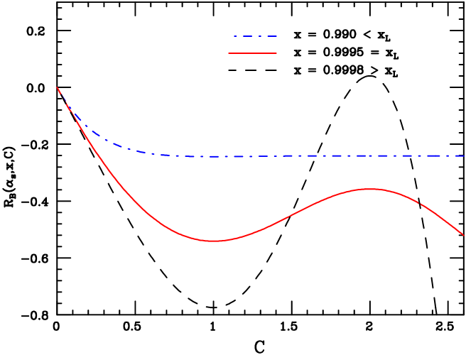
Figure 1: Dependence of the truncated Borel integral $R_{\scriptstyle\rm B}$ eq. (30) on the cutoff $C$ for $\alpha_{s}(Q^{2})=0.25$ and three values of $x$: below, at and above the Landau pole.

The dependence of the value of $R_{\scriptstyle\rm B}(\alpha_{s}(Q^{2}),x,C)$ on $C$ is an $O(\exp-\frac{1}{\alpha_{s}})$ ambiguity in the definition of the asymptotic sum of the divergent series. This dependence is displayed in fig. 1 for three values of $x$, below, at, and above the Landau pole, which at leading order is located at

$$x_{L}=1-e^{-\frac{1}{\beta_{0}\alpha_{s}(Q^{2})}}.$$ (42)

For ease of reference, the dependence of the position $x_{L}$ of the Landau pole on the value of $\alpha_{s}(Q^{2})$ is displayed in fig. 2. Firstly, it is clear from eq. (30) that, because

$$\frac{\partial}{\partial C}R_{\scriptstyle\rm B}(\alpha_{s}(Q^{2}),x,C)=-\frac{1}{\Gamma(1-C)}\,e^{-\frac{C}{\beta_{0}\alpha_{s}(Q^{2}(1-x))}},$$ (43)

the integral has its first stationary point at $C=1$, and then it is stationary at all positive integer values of $C$, where $\Gamma(1-C)$ has simple poles. The first two stationary points are clearly visible in the figure. For $x<x_{L}$, however, $R_{\scriptstyle\rm B}(\alpha_{s}(Q^{2}),x,C)$ has a plateau for $C\mathrel{\mathchoice{\lower 0.86108pt\vbox{\halign{$\m@th\displaystyle\hfil#$\cr>\crcr\sim\crcr}}}{\lower 0.86108pt\vbox{\halign{$\m@th\textstyle\hfil#$\cr>\crcr\sim\crcr}}}{\lower 0.86108pt\vbox{\halign{$\m@th\scriptstyle\hfil#$\cr>\crcr\sim\crcr}}}{\lower 0.86108pt\vbox{\halign{$\m@th\scriptscriptstyle\hfil#$\cr>\crcr\sim\crcr}}}}1$. The origin of this plateau is clear from inspection of eq. (43) again: using eq. (28) it is apparent that $\left|\frac{1}{\Gamma(1-C)}\right|\mathrel{\mathchoice{\lower 0.86108pt\vbox{\halign{$\m@th\displaystyle\hfil#$\cr<\crcr\sim\crcr}}}{\lower 0.86108pt\vbox{\halign{$\m@th\textstyle\hfil#$\cr<\crcr\sim\crcr}}}{\lower 0.86108pt\vbox{\halign{$\m@th\scriptstyle\hfil#$\cr<\crcr\sim\crcr}}}{\lower 0.86108pt\vbox{\halign{$\m@th\scriptscriptstyle\hfil#$\cr<\crcr\sim\crcr}}}}1$ for $C\mathrel{\mathchoice{\lower 0.86108pt\vbox{\halign{$\m@th\displaystyle\hfil#$\cr>\crcr\sim\crcr}}}{\lower 0.86108pt\vbox{\halign{$\m@th\textstyle\hfil#$\cr>\crcr\sim\crcr}}}{\lower 0.86108pt\vbox{\halign{$\m@th\scriptstyle\hfil#$\cr>\crcr\sim\crcr}}}{\lower 0.86108pt\vbox{\halign{$\m@th\scriptscriptstyle\hfil#$\cr>\crcr\sim\crcr}}}}1$, whereas as soon as $x<x_{L}$, $\beta_{0}\alpha_{s}(Q^{2}(1-x))<1$ in the perturbative (large $Q^{2}$) region, so $e^{-\frac{C}{\beta_{0}\alpha_{s}(Q^{2}(1-x))}}\ll 1$. It is only when $C\sim\exp\frac{1}{\beta_{0}\alpha_{s}(Q^{2}(1-x))}\gg 1$ that the factorial growth catches up with the exponential damping. Up to this value of $C$ the growth of $R_{\scriptstyle\rm B}(\alpha_{s}(Q^{2}),x,C)$ with $C$ is negligible.

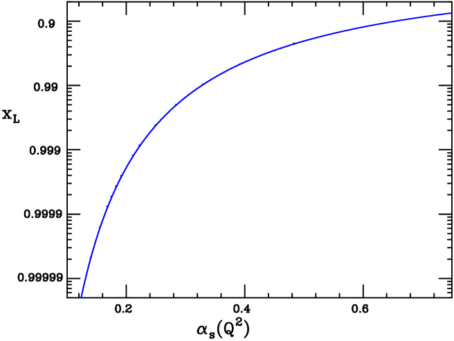
Figure 2: Position of the leading–order Landau pole eq. (42) as a function of $\alpha_{s}(Q^{2})$.

This is as it should be: when $x$ is below the Landau pole, the asymptotic sum of the series is essentially independent of the value of $C$, unless one chooses an unnaturally large or small value. At the Landau pole, a dependence on the value of $C$ appears, due to the fact that if $x\mathrel{\mathchoice{\lower 0.86108pt\vbox{\halign{$\m@th\displaystyle\hfil#$\cr>\crcr\sim\crcr}}}{\lower 0.86108pt\vbox{\halign{$\m@th\textstyle\hfil#$\cr>\crcr\sim\crcr}}}{\lower 0.86108pt\vbox{\halign{$\m@th\scriptstyle\hfil#$\cr>\crcr\sim\crcr}}}{\lower 0.86108pt\vbox{\halign{$\m@th\scriptscriptstyle\hfil#$\cr>\crcr\sim\crcr}}}}x_{L}$ the exponential $O(\exp(1/\alpha_{s}))$ prefactor $e^{-\frac{C}{\beta_{0}\alpha_{s}(Q^{2}(1-x))}}\mathrel{\mathchoice{\lower 0.86108pt\vbox{\halign{$\m@th\displaystyle\hfil#$\cr>\crcr\sim\crcr}}}{\lower 0.86108pt\vbox{\halign{$\m@th\textstyle\hfil#$\cr>\crcr\sim\crcr}}}{\lower 0.86108pt\vbox{\halign{$\m@th\scriptstyle\hfil#$\cr>\crcr\sim\crcr}}}{\lower 0.86108pt\vbox{\halign{$\m@th\scriptscriptstyle\hfil#$\cr>\crcr\sim\crcr}}}}1$, and the concept of asymptotic sum starts losing its meaning. A minimal choice of $C$ is $C=1$, so $R_{\scriptstyle\rm B}$ is stationary for all $x$, and in the beginning of the plateau for $x<x_{L}$.

The physical meaning of $C$ becomes clear by rewriting

$$e^{-\frac{C}{\beta_{0}\alpha_{s}(Q^{2}(1-x))}}=\left(\frac{\Lambda^{2}}{Q^{2}(1-x)}\right)^{C}.$$ (44)

In other words, $R_{ht}(\alpha_{s}(Q^{2}),x,C)$ eq. (36) is a higher twist contribution: the original divergent perturbative series eq. (35) has been made convergent by the inclusion of the higher twist series eq. (36). Of course, eq. (34) implies that this twist series must necessarily also be divergent. Integer values of $C$ correspond to even twists, and in particular if $C=1$, $R_{ht}(\alpha_{s}(Q^{2}),x,C)$ is a standard twist–4 contribution, namely, the first subleading twist. The choice $C=1$ is minimal in that it corresponds to regulating the Borel summation through the first subleading twist.

Equation (44) implies that these higher twist terms are suppressed by powers of $\frac{\Lambda^{2}}{Q^{2}}$, but enhanced by powers of $\frac{1}{1-x}$. The Landau pole is the point where the parameter of the twist expansion is equal to one, i.e., leading twist and higher twist terms are of comparable size. However, despite this enhancement, as long as we choose $C\leq 1$ the Borel sum eq. (30) remains integrable at $x=1$. Indeed, with $C=1$ we have

$$(1-x)R_{\scriptstyle\rm B}(\alpha_{s}(Q^{2}),x,1)=-\int_{0}^{1}dw\,\frac{1}{\Gamma(1-w)}\,e^{-\frac{w}{\beta_{0}\alpha_{s}(Q^{2})}}(1-x)^{1-w},$$ (45)

which vanishes as $x\to 1$ thanks to the fact that $0\leq w\leq 1$. It follows that $P_{\scriptstyle\rm LL}$ eq. (23) with $R$ given by $R_{\scriptstyle\rm B}$ eq.(30) acts as a conventional $+$ distribution, and in particular the integral $\int_{0}^{1}P_{\scriptstyle\rm LL}(\alpha_{s}(Q^{2}),x)f(x)dx$ is finite if the test function $f(x)$ is regular at $x=1$.

When $R_{ht}$ is viewed as a genuine higher twist term, the prefactor $\frac{\Lambda^{2}}{Q^{2}}$ in eq. (36) comes from the Wilson expansion, and not from a factor of $\exp\frac{1}{\alpha_{s}}$, so the higher twist term is just of $O(\alpha_{s})$. However, this term matches an ambiguity in the leading twist, which does not appear at any finite order in the expansion of the leading twist term itself but only in its asymptotic Borel resummation. Equivalently, the higher twist contribution removes the cutoff ambiguity introduced by the need to treat this divergence. The situation is thus akin to the customary case of renormalons, where similarly the ambiguity introduced by the need to make the Borel inversion well–defined is cured by the inclusion of higher twist terms. Henceforth, we will take our result to be given by the Borel sum eq. (30) with $C=1$.

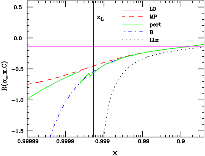
Figure 3: Various determination of the $x$–space resummed result for $\alpha_{s}(Q^{2})=0.25$. LLx denotes the leading $\ln(1-x)$ result of eq. (13), while B, MP and pert denote three different determinations of the divergent leading $\ln N$ series eq. (24), respectively through Borel summation eq. (30) with $C=1$, the minimal prescription eq. (14) and the asymptotic truncation of the perturbative expansion at $K_{0}$ eq. (47). The large–$x$ (constant) leading order result eq. (48) is also shown for comparison.

We now wish to compare this result to the minimal prescription. We do so by defining

$$R_{\scriptstyle\rm MP}(\alpha_{s}(Q^{2}),x)\equiv(1-x)P_{\scriptstyle\rm MP}(\alpha_{s}(Q^{2}),x),$$ (46)

where $P_{\scriptstyle\rm MP}(\alpha_{s}(Q^{2}),x)$ is given by eq. (14). It is clear that the Borel asymptotic sum eq. (30) and the minimal prescription asymptotic sum eq. (46) of the divergent series eq. (27) cannot coincide in general, because the former depends on $C$ and the latter doesn’t. Their $x$–dependence when $C=1$ is compared in fig. 3, where we also show the value of $R$ obtained by truncating the perturbative expansion of the divergent series eq. (27). This is defined by including in $R$ the contribution from the first $K_{0}$ terms in the expansion in powers of $\alpha_{s}(Q^{2})$ eq. (9), where $K_{0}$ is defined as the value where the $k^{th}$ term in the sum in eq. (9), $a_{k}$, starts growing, i.e. as the value $K_{0}$ such that

$$\left|a_{k}+a_{k-1}\right|>\left|a_{k-2}+a_{k-3}\right|\quad\hbox{for}\>\>k>K_{0}.$$ (47)

The definition of the optimal truncation point has some degree of arbitrariness; we have checked that with our choice, eq. (47), the truncated sum is closer to the asymptotic sum than it would be by simply requiring that $\left|a_{k}\right|>\left|a_{k-1}\right|$ for $k>K_{0}$. Note that we have defined the truncation in terms of the expansion eq. (9) in powers of $\alpha_{s}(Q^{2})$, and not in terms of that eq. (27) in powers of $\alpha_{s}(Q^{2}(1-x))$, in order for the truncated result to be well-defined also at the Landau pole $x_{L}$ where $\alpha_{s}(Q^{2}(1-x))$ blows up. For comparison, we also include in fig. 3 the leading $\ln(1-x)$ result eq. (13), and the large $x$ form of the unresummed result, which is simply given by

$$R_{\scriptstyle\rm LO}(\alpha_{s}(Q^{2}),x)=-\beta_{0}\alpha_{s}(Q^{2})+O[(1-x)].$$ (48)

Below the Landau pole the Borel and minimal resummation prescriptions are close to the truncated perturbative result and thus close to each other, as one expects of an asymptotic sum. Note that the leading $\ln(1-x)$ result eq. (13) is reasonably close to these results but never quite on top of them: at not so large $x$, where it reduces to the leading-order result eq. (48), it differs from them because of subleading terms — this is the region were the large $x$ resummation is not very useful. As one enters the large $x$ region, however, the leading $\ln(1-x)$ result eq. (13) is contaminated by the Landau pole where it blows up. So the leading $\ln(1-x)$ result turns out to be of limited usefulness, because there is no region of $x$ where it is applicable. At and above the Landau pole the Borel prescription and the MP prescription start deviating: in this region the higher twist contributions which stabilize the Borel sum are of the same order as the leading twist. On the other hand, at and above the Landau pole the series diverges very fast and its asymptotic sum looses meaningfulness. Hence, comparison of the two prescriptions (Borel and minimal) gives us an estimate of the size of nonperturbative effects: when the two prescriptions start departing from each other, nonperturbative effects become important. Indeed, these two prescriptions bracket the truncated perturbative expansion, which oscillates between them as the order of the truncation (the value of $K_{0}$) varies as a function of $x$.

In summary, we have traced the origin of the divergence of the perturbative expansion of soft gluon resummation, and we have shown that it may be treated by Borel resummation stabilized by higher twist terms. The result that we found is close to the widely adopted minimal prescription, but it deviates from it when nonperturbative corrections become important, namely at the Landau pole. All our computations were presented in the case of threshold resummation (such as e.g. DIS at large $x$) at the leading logarithmic level. The extension to all logarithmic orders and to $p_{T}$ resummation will be discussed elsewhere. Our result is useful for practical calculations in that it does not require the numerical evaluation of a Mellin inversion integral. Furthermore, the availability of more resummation methods that differ in the nonperturbative region is useful in order to assess the reliability of perturbative resummed results.

References

[1]
D. Amati, A. Bassetto, M. Ciafaloni, G. Marchesini and G. Veneziano,
Nucl. Phys. B 173 (1980) 429.
[2]
G. Parisi and R. Petronzio,
Nucl. Phys. B 154 (1979) 427.
[3]
S. Catani, M. L. Mangano, P. Nason and L. Trentadue,
Nucl. Phys. B 478 (1996) 273;
[4]
E. Laenen, J. Smith and W. L. van Neerven,
Nucl. Phys. B 369, 543 (1992).
[5] S. Forte and G. Ridolfi,
Nucl. Phys. B 650 (2003) 229.
[6]
S. Catani and L. Trentadue,
Nucl. Phys. B 327 (1989) 323.
[7]
G. Sterman,
Nucl. Phys. B 281 (1987) 310.
[8] G. Altarelli and G. Parisi,
Nucl. Phys. B 126, 298 (1977).
[9] For a review see e.g.
M. Beneke,
Phys. Rept. 317 (1999) 1.