QCD Multipole Expansion and Hadronic Transitions
in Heavy Quarkonium Systems

Abstract

We review the developments of QCD multipole expansion and its applications to hadronic transitions and some radiative decays of heavy quarkonia. Theoretical predictions are compared with updated experimental results.

I Introduction

Heavy quarkonia are the simplest objects for studying the physics of hadrons due to their nonrelativistic nature. Although the spectra of heavy quarkonium systems $c\bar{c}$ and $b\bar{b}$ have been successfully explained by certain QCD motivated potential models, some of their decays concerning nonperturbative QCD are difficult to deal with. Hadronic transitions

$$\Phi_{I}\to\Phi_{F}+h$$ (1)

are of this kind. In (1), $\Phi_{I}$, $\Phi_{F}$ and $h$ stand for the initial state quarkonium, the final state quarkonium, and the emitted light hadron(s), respectively. Hadronic transitions are important decay modes of heavy quarkonia. For instance, the branching ratio for $\psi^{\prime}\to J/\psi+\pi+\pi$ is approximately $50\%$.

In the $c\bar{c}$ and $b\bar{b}$ systems, the typical mass difference $M_{\Phi_{I}}-M_{\Phi_{F}}$ is around a few hundred MeV, so that the typical momentum of the light hadron(s) $h$ is low. So far as the coupled-channel effect is not concerned, the light hadron(s) $h$ are converted from the gluons emitted by the heavy quark $Q$ or antiquark $\bar{Q}$ in the transition. So the typical momentum of the emitted gluons is also low, and thus perturbative QCD does not work in these processes. Certain nonperturbative approaches are thus needed for studying hadronic transitions. In this article, we review the theoretical framework and applications of a feasible approach, QCD multipole expansion (QCDME), which works quite well in predicting hadronic transition rates in the $c\bar{c}$ and $b\bar{b}$ systems. In addition to hadronic transitions, QCDME can also lead to successful results in certain radiative decay processes such as $J/\psi\to\gamma\eta$ and $J/\psi\to\gamma\eta^{\prime}$.

This paper is organized as follows. In Sec. II, we review the theoretical framework and the formulation of QCDME. Sec. III deals with applications of QCDME to various hadronic transition processes in the nonrelativistic single-channel approach including hadronic transitions between $S$-wave quarkonia, between $P$-wave quarkonia, $\pi\pi$ transition of the $D$-wave quarkonia, and the search for the spin-singlet $P$-wave quarkonium $h_{c}$ through hadronic transition. Sec. IV is on the nonrelativistic coupled-channel theory of hadronic transitions. In Sec, V, we show how QCDME makes successful predictions for the radiative decays $J/\psi\to\gamma\eta$ and $J/\psi\to\gamma\eta^{\prime}$, etc. A summary is given in Sec. VI.

II QCD Multipole Expansion

Multipole expansion in electrodynamics has been widely used for studying radiation processes in which the electromagnetic field is radiated from local sources. If the radius $a$ of a local source is smaller than the wave length $\lambda$ of the radiated electromagnetic field such that $a/\lambda\sim ak<1$ ($k$ stands for the momentum of the photon), $ak$ can be a good expansion parameter, i.e., we can expand the electromagnetic field in powers of $ak$. This is the well-known multipole expansion. In classical electrodynamics, the coefficient of the $(ak)^{l}$ term in the multipole expansion contains a factor $\displaystyle\frac{1}{(2l+1)!!}$. Hence multipole expansion actually works better than what is expected by simply estimating the size of $(ak)^{l}$.

Due to the nonrelativistic nature of heavy quarkonia, the bound states of a heavy quark $Q$ and its antiquark $\bar{Q}$ can be calculated by solving the Schrödinger equation with a given potential model, and the bound states are labelled by the principal quantum number $n$, the orbital angular momentum $L$, the total angular momentum $J$, and the spin multiplicity $\sigma$ ($\sigma=1~{}{\rm or}~{}3$), i.e., $n^{\sigma}L_{J}$. The typical radius $a=\sqrt{\langle r^{2}\rangle}$ of the $c\bar{c}$ and $b\bar{b}$ quarkonia obtained in this way is of the order of $~{}10^{-1}$ fm. With such a small radius, the idea of multipole radiation can be applied to the soft gluon emissions in hadronic transitions. Consider an emitted gluon with a momentum $k$. For typical hadronic transition processes, $k\sim{\rm few~{}hundred~{}MeV}$, so that $~{}ak~{}$ is of the order of $10^{-1}$. Thus multipole expansion works for hadronic transition processes. Note that the convergence of QCDME does not depend on the value of the QCD coupling constant $g_{s}$. Therefore QCDME is a feasible approach to the soft gluon emissions in hadronic transitions (1).

QCDME has been studied by many authors Gottfried ; BR ; Peskin ; VZNS ; Yan ; KYF . The gauge invariant formulation is given in Ref. Yan . Let $\psi(x)$ and $A^{a}_{\mu}(x)$ be the quark and gluon fields, respectively. Following Refs. Yan , we introduce

$$\Psi(\bm{x},t)=U^{-1}(\bm{x},t)\psi(x),$$

$$\frac{\lambda_{a}}{2}A^{a\prime}_{\mu}(\bm{x},t)=U^{-1}(\bm{x},t)\frac{\lambda_{a}}{2}A^{a}_{\mu}(x)U(\bm{x},t)-\frac{i}{g_{s}}U^{-1}(\bm{x},t)\partial_{\mu}U(\bm{x},t),$$ (2)

where $U(\bm{x},t)$ is defined by KYF

$$U(\bm{x},t)\equiv P\exp\bigg{[}ig_{s}\int^{\bm{x}}_{\bm{X}}\frac{\lambda_{a}}{2}{\bm{A}}^{a}(\bm{x}^{\prime},t)\cdot d{\bm{x}}^{\prime}\bigg{]},$$ (3)

in which $P$ is the path-ordering operation, the line integral is along the straight-line segment connecting the two ends, $\bm{X}\equiv(\bm{x}_{1}+\bm{x}_{2})/2$ is the center of mass position of $Q$ and $\bar{Q}$, and $\bm{x}$ denotes $\bm{x_{1}}$ or $\bm{x_{2}}$. With these transformed fields, the part of the QCD Lagrangian related to the heavy quarks becomes Yan

$${\cal L}_{Q} = \int\bar{\Psi}\bigg{[}\gamma^{\mu}\bigg{(}i\partial_{\mu}-g_{s}\frac{\lambda_{a}}{2}A^{a\prime}_{\mu}\bigg{)}-m\bigg{]}\Psi d^{3}x$$ (4)

$$-\frac{1}{2}\frac{g_{s}^{2}}{4\pi}\int\sum^{8}_{a=0}\bar{\Psi}(\bm{x}_{1},t)\gamma^{0}\frac{\lambda_{a}}{2}\Psi(\bm{x}_{1},t)\bigg{|}\frac{1}{\bm{x}_{1}-\bm{x}_{2}}\bigg{|}\bar{\Psi}(\bm{x}_{2},t)\gamma^{0}\frac{\lambda_{a}}{2}\Psi(\bm{x}_{2},t)d^{3}x_{1}d^{3}x_{2},$$

where $\lambda_{0}/2\equiv 1$. Note that the transformed quark field $\Psi(\bm{x},t)$ is dressed with gluons through $U^{-1}(\bm{x},t)$ defined in (3). We see from Eq. (4) that the dressed quark field $\Psi(\bm{x},t)$ serves as the constituent quark field interacting via the static Coulomb potential in the potential model. In addition, it is the transformed gluon field $A^{a\prime}_{\mu}$ (not the original $A^{a}_{\mu}$) that appears in the covariant derivative in (4). $A^{a\prime}_{\mu}$ contains non-Abelian contributions through $U(\bm{x},t)$.

Following Ref. Yan , we generalize the Coulomb potential in Eq. (4) to the static potential including the confining potential in potential models, and we write down the following effective Lagrangian Yan

$${\cal L}^{\rm eff}_{Q} = \int\bar{\Psi}\bigg{[}\gamma^{\mu}\bigg{(}i\partial_{\mu}-g_{s}\frac{\lambda_{a}}{2}A^{a\prime}_{\mu}\bigg{)}-m\bigg{]}\Psi d^{3}x-\frac{1}{2}\int\sum^{8}_{a=0}\bar{\Psi}(\bm{x}_{1},t)\gamma^{0}\frac{\lambda_{a}}{2}\Psi(\bm{x}_{1},t)\bigg{[}\delta_{a0}V_{1}(|\bm{x}_{1}-\bm{x}_{2}|)$$ (5)

$$+(1-\delta_{a0})V_{2}(|\bm{x}_{1}-\bm{x}_{2}|)\bigg{]}\bar{\Psi}(\bm{x}_{2},t)\gamma^{0}\frac{\lambda_{a}}{2}\Psi(\bm{x}_{2},t)d^{3}x_{1}d^{3}x_{2},\hskip 73.97733pt$$

where $V_{1}(|\bm{x_{1}}-\bm{x_{2}}|)$ is the static potential (including the confining potential) between $Q$ and $\bar{Q}$ in the color-singlet state, and $V_{2}(|\bm{x_{1}}-\bm{x_{2}}|)$ is the static potential between $Q$ and $\bar{Q}$ in the color-octet state. This ${\cal L}^{\rm eff}_{Q}$ relates the QCD Lagrangian to the potential models.

Now we consider the multipole expansion. Inside the quarkonium, $|\bm{x-X}|\leq a$. So we can make an expansion by expanding the gluon field $A^{a}_{\mu}(\bm{x},t)$ in Taylor series of $\bm{x-X}$ at the center of mass position $\bm{X}$. The Taylor series is an expansion in powers of the operators $(\bm{x-X})\bm{\cdot}\bm{\nabla}$ and $(\bm{x-X})\bm{\times}\bm{\nabla}$ applying to the gluon field. After operating on the gluon field with the gluon momentum $k$, these operators are of the order of $ak$. This is QCDME. It has been shown in Ref. Yan that this operation leads to

$$A^{a\prime}_{0}(\bm{x},t)=A^{a\prime}_{0}(\bm{X},t)-(\bm{x}-\bm{X})\bm{\cdot}{\bm{E}}^{a}(\bm{X},t)+\cdots,$$ (6)

$${\bm{A}}^{a\prime}(\bm{x},t)=-\frac{1}{2}(\bm{x}-\bm{X})\bm{\times}{\bm{B}}^{a}(\bm{X},t)+\cdots,\hskip 28.45274pt$$ (7)

where ${\bm{E}}^{a}$ and ${\bm{B}}^{a}$ are color-electric and color-magnetic fields, respectively.

In Ref. Yan , the corresponding Hamiltonian was derived based on the above formulation. This is more convenient in using the nonrelativistic perturbation theory. The obtain Hamiltonian is Yan

$$H^{\rm eff}_{QCD}=H^{(0)}_{QCD}+H^{(1)}_{QCD},$$ (8)

where

$$H^{(0)}_{QCD} = \int\Psi^{\dagger}(\bm{x}_{1},t)\Psi(\bm{x}_{1},t)\hat{H}\Psi^{\dagger}(\bm{x}_{2},t)\Psi(\bm{x}_{2},t)d^{3}x_{1}d^{3}x_{2}$$ (9)

with

$$\hat{H}\equiv-\frac{1}{2m_{Q}}(\partial_{1}^{2}+\partial_{2}^{2}+V_{1}(|\bm{x}_{1}-\bm{x}_{2}|)+\sum^{8}_{a=1}\frac{\lambda_{a}}{2}\frac{\bar{\lambda}_{a}}{2}V_{2}(|\bm{x}_{1}-\bm{x}_{2}|)+2m_{Q},$$ (10)

and

$$H^{(1)}_{QCD} = H_{1}+H_{2},$$ (11)

$$H_{1}\equiv Q_{a}A^{a}_{0}(\bm{X},t),~{}~{}~{}~{}~{}~{}H_{2}\equiv-{\bm{d}}_{a}\bm{\cdot}{\bm{E}}^{a}(\bm{X},t)-{\bm{m}}_{a}\bm{\cdot}{\bm{B}}^{a}(\bm{X},t)+\cdots,\hskip 14.22636pt$$

in which

$$Q_{a}\equiv g_{E}\int\Psi^{\dagger}(\bm{x},t)\frac{\lambda_{a}}{2}\Psi(\bm{x},t)d^{3}x,$$ (12)

$${\bm{d}}_{a}\equiv g_{E}\int(\bm{x}-\bm{X})\Psi^{\dagger}(\bm{x},t)\frac{\lambda_{a}}{2}\Psi(\bm{x},t)d^{3}x,$$ (13)

$${\bm{m}}_{a}\equiv\frac{g_{M}}{2}\int(\bm{x}-\bm{X})\bm{\times}\Psi^{\dagger}(\bm{x},t){\bm{\gamma}}\frac{\lambda_{a}}{2}\Psi(\bm{x},t)d^{3}x$$ (14)

are the color charge, color-electric dipole moment, and color-magnetic dipole moment of the $Q\bar{Q}$ system, respectively. Note that Eq. (5) is regarded as an effective Lagrangian. Considering that the heavy quark may have an anomalous magnetic moment, we have taken in Eqs. (12), (13) and (14) the symbols $g_{E}$ and $g_{M}$ to denote the effective coupling constants for the electric and magnetic multipole gluon emissions, respectively. We shall see later in Sec. III that taking $\alpha_{E}$ and $\alpha_{M}$ as two parameters is needed phenomenologically.

We are going to take $H^{(0)}_{QCD}$ as the zeroth order Hamiltonian, and take $H^{(1)}_{QCD}$ as a perturbation. This is different from the ordinary perturbation theory since $H^{(0)}_{QCD}$ is not a free field Hamiltonian. $H^{(0)}_{QCD}$ contains strong interactions in the potentials in $\hat{H}$, so that the eigenstates of $H^{(0)}_{QCD}$ are bound states rather than free field states. For a given potential model, the zeroth order solution can be obtained by solving the Schrödinger equation with the given potential. Moreover, we see from Eqs. (12), (13) and (14) that only $H_{2}$ in $H^{(1)}_{QCD}$ is of $O(ak)$, while $H_{1}$ is of $O((ak)^{0})$. So that we should keep all orders of $H_{1}$ in the perturbation expansion.

The general formula for the $S$ matrix element between the initial state $|I\rangle$ and the final state $|F\rangle$ in this expansion has been given in Ref. KYF , which is

$$\langle F|S|I\rangle=-i2\pi\delta(E_{F}+\omega_{F}-E_{I})\bigg{<}F~{}\bigg{|}H_{2}\frac{1}{E_{I}-H^{(0)}_{QCD}+i\partial_{0}-H_{1}}H_{2}\cdots H_{2}\frac{1}{E_{I}-H^{(0)}_{QCD}+i\partial_{0}-H_{1}}H_{2}\bigg{|}~{}I\bigg{>},$$ (15)

where $\omega_{F}$ is the energy of the emitted gluons. This is the basis of the study of hadronic transitions in QCDME. Explicit evaluation of the $S$ matrix elements in various cases will be presented in Sec. III.

III Predictions for Hadronic Transitions in the Single-Channel approach

In this section, we shall show the predictions for hadronic transitions rates in the single-channel approach (inclusion of coupled-channel contributions will be given in Sec. IV). In this approach, the amplitude of hadronic transitions (1) is diagrammatically shown in FIG. 1 in which there are two complicated vertices: namely, the vertex of multipole gluon emissions (MGE) from the heavy quarks and the vertex of hadronization (H) describing the conversion of the emitted gluons into light hadron(s). The MGE vertex is at the scale of the heavy quarkonium, and it depends on the property of the heavy quarkonium. The H vertex is at the scale of the light hadron(s), and is independent of the property of the heavy quarkonium. In the following, we shall treat them separately.

Figure 1: Diagram for a typical hadronic transition in the single-channel approach.

III.1 Hadronic Transitions Between $\bm{S}$-Wave Quarkonia

Let us first consider the case of $\pi\pi$ transitions between $S$-wave quarkonia, $n_{I}^{3}S_{1}\to n_{F}^{3}S_{1}+\pi+\pi$. These processes are dominated by double electric-dipole transitions (E1E1). The transition amplitude can be obtained from the $S$ matrix element (15). With certain algebra, we obtain KYF ; Yan ; KY81

$${\cal M}_{E1E1}=i\frac{g_{E}^{2}}{6}\bigg{<}\Phi_{F}h\bigg{|}{\bm{\bar{x}}}\cdot{\bm{E}}\frac{1}{E_{I}-H^{(0)}_{QCD}-iD_{0}}{\bm{\bar{x}}}\cdot{\bm{E}}\bigg{|}\Phi_{I}\bigg{>},$$ (16)

where $\bm{\bar{x}}$ is the separation between $Q$ and $\bar{Q}$, and $(D_{0})_{bc}\equiv\delta_{bc}\partial_{0}-g_{s}f_{abc}A^{a}_{0}$. Let us insert a complete set of intermediate states with the principal quantum number $K$ and the orbital angular momentum $L$. Then Eq. (16) can be written as

$${\cal M}_{E1E1}=i\frac{g_{E}^{2}}{6}\sum_{KLK^{\prime}L^{\prime}}\bigg{\langle}\Phi_{F}h\bigg{|}{\bm{\bar{x}}}\cdot{\bm{E}}\bigg{|}KL\bigg{\rangle}\bigg{\langle}KL\bigg{|}\frac{1}{E_{I}-H^{(0)}_{QCD}-iD_{0}}\bigg{|}K^{\prime}L^{\prime}\bigg{\rangle}\bigg{\langle}K^{\prime}L^{\prime}\bigg{|}{\bm{\bar{x}}}\cdot{\bm{E}}\bigg{|}\Phi_{I}\bigg{\rangle},$$ (17)

According to the angular momentum selection rule, the intermediate states must have $L=L^{\prime}=1$. The intermediate states in the hadronic transition are the states after the emission of the first gluon and before the emission of the second gluon shown in FIG. 1, i.e. they are states with a gluon and a color-octet $Q\bar{Q}$. There is strong interaction between the gluon and the color-octet $Q\bar{Q}$ since they all carry colors. Thus these states are the so-called hybrid states. It is difficult to calculate these hybrid states from the first principles of QCD. So we shall take a reasonable model for it. The model should reasonably reflect the main properties of the hybrid states and should contain as few unknown parameters as possible in order not to affect the predictive power of the theory. There is a quark confining string (QCS) model QCS satisfying these requirements. The QCS model is a one dimensional string model in which the strong confining force between $Q$ and $\bar{Q}$ is described by the ground-state string, and gluon excitation effects are described by the vibrations of the string QCS . Our intermediate states $Q\bar{Q}g$ are thus described by the first vibrational mode in this model. The QCS model is not the only one satisfying the above requirements. Another possible model satisfying the requirements is the MIT bag model for the hybrid states. Hadronic transitions with the MIT bag model as the model for the intermediate states has been studied in Ref. bag . It is shown that, with the same input data, the predictions in this model are very close to those in the QCS model although the absolute intermediate state energy eigenvalues in the bag model are much higher than those in the QCS model. Thus the predictions are not sensitive to the specific energy spectrum of the intermediate states. In the following, we take the calculations with the QCS model as examples. Explicit calculations of the first vibrational mode as the intermediate states is given in Ref. KY81 . With this model, the transition amplitude (17) becomes KY81

$${\cal M}_{E1E1}=i\frac{g_{E}^{2}}{6}\sum_{KL}\frac{\langle\Phi_{F}|\bar{x}_{k}|KL\rangle\langle KL|\bar{x}_{l}|\Phi_{I}\rangle}{E_{I}-E_{KL}}\langle\pi\pi|E^{a}_{k}E^{a}_{l}|0\rangle,$$ (18)

where $E_{KL}$ is the energy eigenvalue of the intermediate vibrational state $|KL\rangle$. We see that, in this approach, the transition amplitude contains two factors: namely, the heavy quark MGE factor (the summation) and the H factor $\langle\pi\pi|E^{a}_{k}E^{a}_{l}|0\rangle$. The first factor concerns the wave functions and energy eigenvalues of the initial and final state quarkonia and the intermediate states. These can be calculated for a given potential model. Let us now consider the treatment of the second factor. The scale of the H factor is the scale of light hadrons which is very low. Therefore the calculation of this matrix element is highly nonperturbative. So far, there is no reliable way of calculating this H factor from the first principles of QCD. Therefore we take a phenomenological approach based on an analysis of the structure of this matrix element using PCAC and soft pion technique in Ref. BrownCahn . In the center-of-mass frame, the two pion momenta $q_{1}$ and $q_{2}$ are the only independent variables describing this matrix element. According Ref. BrownCahn , we can write this matrix element as KY81

$$\frac{g_{E}^{2}}{6}\langle\pi_{\alpha}(q_{1})\pi_{\beta}(q_{2})|E^{a}_{k}E^{a}_{l}|0\rangle=\frac{\delta_{\alpha\beta}}{\sqrt{(2\omega_{1})(2\omega_{2})}}\bigg{[}C_{1}\delta_{kl}q^{\mu}_{1}q_{2\mu}+C_{2}\bigg{(}q_{1k}q_{2l}+q_{1l}q_{2k}-\frac{2}{3}\delta_{kl}{\bm{q}}_{1}\cdot{\bm{q}}_{2}\bigg{)}\bigg{]},$$ (19)

where $C_{1}$ and $C_{2}$ are two unknown constants. In the rest frame of $\Phi_{I}$ (the center-of-mass frame), for a given $\pi\pi$ invariant mass $M_{\pi\pi}$, the $C_{1}$ term is isotropic ($S$-wave), while the $C_{2}$ term is angular dependent ($D$-wave). In the nonrelativistic single-channel approach, the MGE factor in (18) is proportional to $\delta_{kl}$ due to orbital angular momentum conservation. So that only the $C_{1}$ term contributes to the $S$-state to $S$-state transitions. In this case, the $n_{I}^{3}S_{1}\to n_{F}^{3}S_{1}+\pi+\pi$ transition rate can be expressed as KY81

$$\Gamma(n_{I}^{3}S_{1}\to n_{F}^{3}S_{1}~{}\pi~{}\pi)=|C_{1}|^{2}G|f^{111}_{n_{I}0n_{F}0}|^{2},$$ (20)

where the phase-space factor $G$ is KY81

$$G\equiv\frac{3}{4}\frac{M_{\Phi_{F}}}{M_{\Phi_{I}}}\pi^{3}\int K\sqrt{1-\frac{4m_{\pi}^{2}}{M_{\pi\pi}^{2}}}(M_{\pi\pi}^{2}-2m_{\pi}^{2})^{2}~{}dM_{\pi\pi}^{2},$$ (21)

with

$$~{}~{}K\equiv\frac{\sqrt{(M_{\Phi_{I}}+M_{\Phi_{F}})^{2}-M_{\pi\pi}^{2}}\sqrt{(M_{\Phi_{I}}-M_{\Phi_{F}})^{2}-M_{\pi\pi}^{2}}}{2M_{\Phi_{I}}},$$ (22)

and

$$f^{LP_{I}P_{F}}_{n_{I}l_{I}n_{F}l_{F}}\equiv\sum_{K}\frac{\int R_{F}(r)r^{P_{F}}R^{*}_{KL}(r)r^{2}dr\int R^{*}_{KL}(r^{\prime})r^{\prime P_{I}}R_{I}(r^{\prime})r^{\prime 2}dr^{\prime}}{M_{I}-E_{KL}},$$ (23)

in which $R_{I}$, $R_{F}$, and $R_{KL}$ are radial wave functions of the initial, final, and intermediate vibrational states, respectively. These radial wave functions are calculated from the Schrödinger equation with a given potential model.

Now there is only one overall unknown constant $C_{1}$ left in this transition amplitude, and it can be determined by taking a well-measured hadronic transition rate as an input. So far, the best measured $S$-state to $S$-state $\pi\pi$ transition rate is $\Gamma(\psi^{\prime}\to J/\psi~{}\pi\pi)$. The updated experimental value is PDG

$$\Gamma_{\rm tot}(\psi^{\prime})=281\pm 17~{}{\rm keV},$$

$$B(\psi^{\prime}\to J/\psi~{}\pi^{+}\pi^{-})=(31.8\pm 1.1)\%,$$

$$B(\psi^{\prime}\to J/\psi~{}\pi^{0}\pi^{0})=(18.8\pm 1.2)\%.$$ (24)

We take this as an input to determine $C_{1}$. Then we can predict all the $S$-state to $S$-state $\pi\pi$ transitions rates in the $\Upsilon$ system. Since the transition rate (20) depends on the potential model through the amplitude (23), the determined value of $|C_{1}|$ is model dependent. In the following, we take the Cornell Coulomb plus linear potential model Cornell and the Buchmüller-Grunberg-Tye (BGT) potential model BGT as examples to show the determined $|C_{1}|$ and the predicted rates of $\Upsilon^{\prime}\to\Upsilon~{}\pi\pi$, $\Upsilon^{\prime\prime}\to\Upsilon~{}\pi\pi$, and $\Upsilon^{\prime\prime}\to\Upsilon^{\prime}~{}\pi\pi$. The results are listed in TABLE I .

Table 1: The determined $|C_{1}|^{2}$ and the predicted rates $\Gamma(\Upsilon^{\prime}\to\Upsilon~{}\pi\pi)$, $\Gamma(\Upsilon^{\prime\prime}\to\Upsilon~{}\pi\pi)$, and $\Gamma(\Upsilon^{\prime\prime}\to\Upsilon^{\prime}~{}\pi\pi)$ ( in keV) in the Cornell model and the BGT model. The corresponding updated experimental values of the transition rates quoted from Ref. PDG are also listed for comparison.

	Cornell	BGT	Expt.
$|C_{1}|^{2}\hskip 79.6678pt$	$83.4\times 10^{-6}$	$67.8\times 10^{-6}$
$\Gamma(\Upsilon^{\prime}\to\Upsilon\pi\pi)$ (keV)	8.6	7.8	$~{}~{}~{}12.0~{}\pm 1.8~{}~{}~{}~{}~{}~{}$
$\Gamma(\Upsilon^{\prime\prime}\to\Upsilon\pi\pi)$ (keV)	0.44	1.2	$1.72\pm 0.35$
$\Gamma(\Upsilon^{\prime\prime}\to\Upsilon^{\prime}\pi\pi)$ (keV)	0.78	0.53	$1.26\pm 0.40$

We see that the predicted ratios $\Gamma(\Upsilon^{\prime\prime}\to\Upsilon~{}\pi\pi)/\Gamma(\Upsilon^{\prime}\to\Upsilon~{}\pi\pi)\approx 1.2/7.8=0.15$  and   $\Gamma(\Upsilon^{\prime\prime}\to\Upsilon^{\prime}~{}\pi\pi)/\Gamma(\Upsilon^{\prime}\to\Upsilon~{}\pi\pi)\approx 0.53/7.8=0.07$ in the BGT model are close to the corresponding experimental values $\Gamma(\Upsilon^{\prime\prime}\to\Upsilon~{}\pi\pi)/\Gamma(\Upsilon^{\prime}\to\Upsilon~{}\pi\pi)\approx 1.72/12.0=0.14$ and $\Gamma(\Upsilon^{\prime\prime}\to\Upsilon^{\prime}~{}\pi\pi)/\Gamma(\Upsilon^{\prime}\to\Upsilon~{}\pi\pi)\approx 1.26/12.0=0.11$. However, the predicted absolute partial widths are smaller than the corresponding experimental values by roughly a factor of $(50\--75)\%$. Moreover, when the $M_{\pi\pi}$ distributions are considered, the situation will be more complicated. We shall deal with these issues in Sec. IV.

Note that the phase space factor $G$ in $\Upsilon^{\prime\prime}\to\Upsilon~{}\pi\pi$ is much larger than that in $\Upsilon^{\prime}\to\Upsilon~{}\pi\pi$, $G(\Upsilon^{\prime\prime}\to\Upsilon~{}\pi\pi)/G(\Upsilon^{\prime}\to\Upsilon~{}\pi\pi)=33$. So one may naively expect that $\Gamma(\Upsilon^{\prime\prime}\to\Upsilon~{}\pi\pi)>\Gamma(\Upsilon^{\prime}\to\Upsilon~{}\pi\pi)$. However, as we see from the experimental values in TABLE I that $\Gamma(\Upsilon^{\prime\prime}\to\Upsilon~{}\pi\pi)/\Gamma(\Upsilon^{\prime}\to\Upsilon~{}\pi\pi)\approx 1.72/12.2=0.14$. The reason why our predictions for this ratio is close to the experimental value is that the contributions from various intermediate states to the overlapping integrals in the summation in $f^{111}_{3010}$ [cf. Eq. (23)] drastically cancel each other due to the fact that the $\Upsilon^{\prime\prime}$ wave function contains two nodes. This is a characteristic of this kind of intermediate state models (QCS or bag model). To see this, let us take a simplified model for the intermediate states and look at its prediction. If we make a simplification assumption that the variation of the factor $1/(E_{I}-H^{(0)}_{QCD}-iD_{0})$ in Eq. (17) is sufficiently slow such that it can be approximately represented by a constant which can be taken out of the summation, the summations $\displaystyle\sum_{KL}$ and $\displaystyle\sum_{K^{\prime}L^{\prime}}$ in (17) can then be carried out and the double overlapping integrals in the numerator in (23) reduces to a single integration $\int R^{*}_{\Upsilon^{\prime\prime}}(r)r^{2}R_{\Upsilon}(r)r^{2}dr$. This simplified model predicts a rate $\Gamma(\Upsilon^{\prime\prime}\to\Upsilon~{}\pi\pi)$ larger than the experimental value by orders of magnitude KY81 . Therefore, taking a reasonable model for the intermediate states is crucial for obtaining successful predictions in the QCDME approach to the MGE factor.

The transitions $~{}n_{I}^{3}S_{1}\to n_{F}^{3}S_{1}+\eta~{}$ are contributed by E1M2 and M1M1 transitions, and is dominated by the E1M2 transition. The transition amplitude is

$${\cal M}_{E1M2}=-\frac{i}{2m_{Q}}\frac{g_{E}g_{M}}{6}\sum_{KL}\frac{\langle\Phi_{F}|\bar{x}_{k}|KL\rangle\langle KL|S_{l}\bar{x}_{m}|\Phi_{I}\rangle+\langle\Phi_{F}|S_{l}\bar{x}_{m}|KL\rangle\langle KL|\bar{x}_{k}|\Phi_{I}\rangle}{E_{I}-E_{KL}}\langle\eta|E^{a}_{k}\partial_{m}B^{a}_{l}|0\rangle,$$ (25)

where $\bm{S}$ is the total spin of the quarkonium. The MGE matrix element is proportional to $\delta_{km}$. Similar to the idea in (19), we can phenomenologically parameterize the hadronization factor according to its Lorentz structure as KTY88

$$\frac{g_{E}g_{M}}{6}\langle\eta(q)|E^{a}_{k}\partial_{k}B^{a}_{l}|0\rangle=i(2\pi)^{3/2}~{}C_{3}~{}q_{l},$$ (26)

in which the phenomenological constant can be determined by taking the data PDG

$$\Gamma_{\rm tot}(\psi^{\prime})=277\pm 22~{}{\rm keV},~{}~{}~{}~{}~{}~{}~{}~{}B(\psi^{\prime}\to J/\psi~{}\eta)=(3.17\pm 0.21)\%$$ (27)

as input, and so we can predict the rates for $\Upsilon^{\prime}\to\Upsilon~{}\eta$ and $\Upsilon^{\prime\prime}\to\Upsilon~{}\eta$. This is equivalent to

$$\Gamma(\Upsilon(n_{I}^{3}S_{1})\to\Upsilon~{}\eta)=\displaystyle\frac{\bigg{|}\displaystyle\frac{f^{111}_{n_{I}010}(b\bar{b})}{m_{b}}\bigg{|}^{2}}{\bigg{|}\displaystyle\frac{f^{111}_{2010}(c\bar{c})}{m_{c}}\bigg{|}^{2}}\frac{|{\bm{q}}(b\bar{b)}|^{3}}{|{\bm{q}}(c\bar{c})|^{3}}\Gamma(\psi^{\prime}\to J/\psi~{}\eta).$$ (28)

where $\bm{q}(b\bar{b})$ and $\bm{q}(c\bar{c})$ are the momenta of $\eta$ in $\Upsilon(n_{I}^{3}S_{1})\to\Upsilon~{}\eta$ and $\psi^{\prime}\to J/\psi~{}\eta$, respectively. Taking the BGT model as an example to calculate the ratio of transition amplitudes in (28), we obtained

$$\Gamma(\Upsilon^{\prime}\to\Upsilon~{}\eta)=0.022~{}{\rm keV},~{}~{}~{}~{}~{}~{}\Gamma(\Upsilon^{\prime\prime}\to\Upsilon~{}\eta)=0.011~{}{\rm keV}.$$ (29)

These are consistent with the present experimental bounds PDG

$$\Gamma(\Upsilon^{\prime}\to\Upsilon~{}\eta)<0.086~{}{\rm keV},~{}~{}~{}~{}~{}~{}\Gamma(\Upsilon^{\prime\prime}\to\Upsilon`~{}\eta)<0.058~{}{\rm keV}.$$ (30)

We can also compare the ratios $R^{\prime}\equiv\Gamma(\Upsilon^{\prime}\to\Upsilon~{}\eta)/\Gamma(\psi^{\prime}\to J/\psi~{}\eta)$ and $R^{\prime\prime}\equiv\Gamma(\Upsilon^{\prime\prime}\to\Upsilon~{}\eta)/\Gamma(\psi^{\prime}\to J/\psi~{}\eta)$ with the recent experimental measurements. Recently BES has obtained an accurate measurement of $\Gamma(\psi^{\prime}\to J/\psi~{}\eta)$ and $\Gamma(\psi^{\prime}\to J/\psi~{}\pi^{0})$ besggJ . With the new BES data and the bounds on $\Gamma(\Upsilon^{\prime}\to\Upsilon~{}\eta)$ and $\Gamma(\Upsilon^{\prime\prime}\to\Upsilon~{}\eta)$ PDG , the experimental bounds on $R^{\prime}$ and $R^{\prime\prime}$ are besggJ

$$R^{\prime}|_{expt}<0.0098,~{}~{}~{}~{}R^{\prime\prime}|_{expt}<0.0065.$$ (31)

Taking the BGT model to calculate the ratios $R^{\prime}$ and $R^{\prime\prime}$, we obtain

$$R^{\prime}|_{BGT}=0.0025,~{}~{}~{}~{}~{}~{}~{}~{}~{}~{}R^{\prime\prime}|_{BGT}=0.0013.$$ (32)

These are consistent with the new experimental bounds (31).

III.2 $\bm{\pi}\bm{\pi}$ Transitions Between $\bm{P}$-Wave Quarkonia

Let us consider the hadronic transitions $2^{3}P_{J_{I}}\to 1^{3}P_{J_{F}}+\pi+\pi$. For simplicity, we use the symbol $\Gamma(J_{I}\to J_{F})$ to denote $\Gamma(2^{3}P_{J_{I}}\to 1^{3}P_{J_{F}}\pi\pi)$. These are also dominated by E1E1 transitions. The obtained results are Yan ; KY81

$$\Gamma(0\to 0)=\frac{1}{9}|C_{1}|^{2}G\bigg{|}f^{011}_{2111}+2f^{211}_{2111}\bigg{|}^{2},~{}~{}~{}~{}\Gamma(0\to 1)=\Gamma(1\to 0)=0,$$

$$\Gamma(0\to 2)=5\Gamma(2\to 0)=\frac{10}{27}|C_{2}|^{2}H\bigg{|}f^{011}_{2111}+\frac{1}{5}f^{211}_{2111}\bigg{|}^{2},~{}~{}~{}~{}\Gamma(1\to 1)=\Gamma(0\to 0)+\frac{1}{4}\Gamma(0\to 2),$$

$$\Gamma(1\to 2)=\frac{5}{3}\Gamma(2\to 1)=\frac{3}{4}\Gamma(0\to 2),~{}~{}~{}~{}\Gamma(2\to 2)=\Gamma(0\to 0)+\frac{7}{20}\Gamma(0\to 2),$$ (33)

where the phase-space factor $H$ is

$$H=\frac{1}{20}\frac{M_{\Phi_{F}}}{M_{\Phi_{I}}}\pi^{3}\int K\sqrt{1-\frac{4m_{\pi}^{2}}{M_{\pi\pi}}}\bigg{[}(M_{\pi\pi}^{2}-4m_{\pi}^{2})^{2}\bigg{(}1+\frac{2}{3}\frac{K^{2}}{M_{\pi\pi}^{2}}\bigg{)}+\frac{8K^{4}}{15M_{\pi\pi}^{4}}(M_{\pi\pi}^{4}+2m_{\pi}^{2}M_{\pi\pi}^{2}+6m_{\pi}^{4})\bigg{]}~{}dM_{\pi\pi}^{2},$$ (34)

with $K$ defined in Eq. (22).

Now the rates in (33) depend on both $C_{1}$ and $C_{2}$. We know that $C_{1}$ has been determined by the input (24). So far, there is no well measured hadronic transition rate available for determining the ratio $C_{2}/C_{1}$. At present, to make predictions, we can only take certain approximation to estimate $C_{2}/C_{1}$ theoretically. The approximation taken in Ref. KY81 is to assume that the H factor $\langle\pi\pi|E^{a}_{k}E^{a}_{l}|0\rangle$ can be approximately expressed as

$$\langle\pi\pi|E^{a}_{k}E^{a}_{l}|0\rangle\propto\langle gg|E^{a}_{k}E^{a}_{l}|0\rangle,$$ (35)

i.e., $\langle\pi\pi|E^{a}_{k}E^{a}_{l}|0\rangle$ approximately contains a factor $\langle gg|E^{a}_{k}E^{a}_{l}|0\rangle$ and another factor describing the conversion of the two gluons into $\pi\pi$ which is assumed to be approximately independent of the pion momenta in the hadronic transitions under consideration. The R.H.S. of Eq. (35) can be easily calculated. Comparing the obtained result with the form (19), we obtain

$$C_{2}/C_{1}\approx 3$$ (36)

in such an approximation. This is a crude approximation which can only be regarded as an order of magnitude estimate. So it is likely that $C_{2}/C_{1}\sim O(1)$ rather than $O(10^{-1})$ or $O(10)$. A reasonable range of $C_{2}/C_{1}$ is

$$1\lesssim C_{2}/C_{1}\lesssim 3.$$ (37)

With this range of $C_{2}/C_{1}$, the obtained transition rates $\Gamma(J_{I}\to J_{F})$ of $\chi_{b}(2^{3}P_{J_{I}})\to\chi_{b}(1^{3}P_{J_{F}})\pi\pi$ in the Cornell model Cornell and the BGTmodel BGT are listed in TABLE II. The relations between different $\Gamma(J_{I}\to J_{F})$ given in Eq. (33) reflect the symmetry in the E1E1 multipole expansion Yan , so that experimental tests of these relations are of special interest. Recently, CLEO reported a preliminary observation of the hadronic transitions $\chi_{b}(2^{3}P_{J_{I}})\to\chi_{b}(1^{3}P_{J_{F}})\pi\pi$ for $J_{I}=J_{F}=1$ and 2 Skwarnicki05 . In a very recent paper Cawlfield , CLEO measured the transition rate, and the obtained result is $\Gamma(\chi_{b}(2^{3}P_{J_{I}})\to\chi_{b}(1^{3}P_{J_{F}})\pi\pi)=(0.83\pm 0.22\pm 0.08\pm 0.19)$ keV ($J_{I}=J_{F}=1,~{}2$) which is consistent with the predicted rates $\Gamma(1\to 1)$, and $\Gamma(2\to 2)$ listed in TABLE 2.

Table 2: Predicted transition rates $\Gamma(J_{I}\to J_{F})$ of $\chi_{b}(2^{3}P_{J_{I}})\to\chi_{b}(1^{3}P_{J_{F}})\pi\pi$ with the parameter range (37) in the Cornell model Cornell and the BGTmodel BGT .

Model $\Gamma(J_{I}\to J_{F})$ (keV) $\Gamma(0\to 0)$ $\Gamma(0\to 2)$ $\Gamma(1\to 1)$ $\Gamma(1\to 2)$ $\Gamma(2\to 2)$ Cornell 0.4 0.004$\--$0.04 0.4 0.003$\--$0.03 0.4 BGT 0.4 0.002$\--$0.02 0.4 0.001$\--$0.01 0.4

III.3 $\bm{\pi}\bm{\pi}$ Transitions of $\bm{D}$-Wave Quarkonia

$\psi(3770)$ (or $\psi^{\prime\prime}$) is commonly regarded as essentially the $1D$ state of the charmonium. It lies above the $D\bar{D}$ threshold, so that it is usually believed that $\psi(3770)$ mainly decays into the open channel $D\bar{D}$. Experimental observations show that the directly measured $\psi(3770)$ production cross section at $e^{+}e^{-}$ colliders is CrystalBall84 ; MARKII

$$\sigma(\psi(3770))=7.5\pm 0.8~{}{\rm nb},$$ (38)

while the $e^{+}e^{-}\to\psi(3770)\to D\bar{D}$ cross section is MARKIII

$$\sigma(\psi(3770)\to D\bar{D})=5.0\pm 0.5~{}{\rm nb}.$$ (39)

This discrepancy may indicate that there are considerable non-$D\bar{D}$ decay modes of $\psi(3770)$. One of the possible non-$D\bar{D}$ decay modes is the hadronic transition $\psi(3770)\to J/\psi~{}\pi\pi$. Theoretical studies of hadronic transitions of the $D$-wave quarkonia have been carried out by several authors in different approaches leading to quite different predictions BLMN ; KY81 ; MoxhayKo ; KY90 ; Kuang02 . In the following, we briefly review the approach given in Refs. KY90 ; Kuang02 , and compare the predictions with the recent experimental result and with other approaches.

The measured leptonic width of $\psi(3770)$ is $(0.26\pm 0.04)$ keV PDG . If we simply regard $\psi(3770)$ as a pure $1D$ state of charmonium, the predicted leptonic width will be smaller than the experimental value by an order of magnitude. Therefore people consider $\psi(3770)$ as a mixture of charmonium states KY90 ; Kuang02 ; Godfrey . State mixing is an important consequence of the coupled-channel theory, especially for states close to or beyond the open channel threshold. Take a successful coupled-channel model, the unitary quark model (UQM) UQM , as an example. In this model, $\psi(3770)$ is a mixture of many $S$-wave and $D$-wave states of charmonium, but the main ingredients are the $\psi(1D)$ and $\psi(2S)$ states. Neglecting the small ingredients, we can write $\psi^{\prime}$ and $\psi(3770)$ as

$$\psi^{\prime}=\psi(2S)\cos\theta+\psi(1D)\sin\theta,$$

$$\psi(3770)=-\psi(2S)\sin\theta+\psi(1D)\cos\theta.$$ (40)

The UQM gives $\theta\approx-8^{\circ}$ UQM . Instead of taking a specific coupled-channel model, we take a phenomenological approach determining the mixing angle $\theta$ by fitting the ratio of the leptonic width of $\psi^{\prime}$ and $\psi(3770)$. The leptonic widths of $\psi(2S)$ and $\psi(1D)$ are proportional to the wave function at the origin $\psi_{2S}(0)$ and the second derivative of the wave function at the origin $\displaystyle\frac{5}{\sqrt{2}}\frac{d^{2}\psi_{1D}(0)/dr^{2}}{2m_{c}^{2}}$, respectively. Therefore the determination of $\theta$ depends on the potential model. Here we take two potential models as illustration: namely, the Cornell potential model Cornell and the improved QCD motivated potential model by Chen and Kuang (CK) CK92 which leads to more successful phenomenological results. The determined values of $\theta$ are

$${\rm Cornell}:~{}~{}\theta=-10^{\circ},$$

$${\rm CK}:~{}~{}~{}~{}~{}~{}~{}\theta=-12^{\circ}.$$ (41)

These are all consistent with the UQM value. There can also be an alternative solution with $\theta\sim 30^{\circ}$, but it is ruled out by the measured $M_{\pi\pi}$ distribution of $\psi^{\prime}\to J/\psi+\pi+\pi$.

This transition is also dominated by E1E1 gluon emission. The transition rate is KY90

$$\Gamma\big{(}\psi(3770)\to J/\psi~{}\pi\pi\big{)}=|C_{1}|^{2}\bigg{[}\sin^{2}\theta~{}G(\psi^{\prime})~{}|f^{111}_{2010}(\psi^{\prime})|^{2}+\frac{4}{15}\bigg{|}\frac{C_{2}}{C_{1}}\bigg{|}^{2}\cos^{2}\theta~{}H(\psi^{\prime\prime})~{}|f^{111}_{1210}(\psi^{\prime\prime})|^{2}\bigg{]}.$$ (42)

This transition rate depends on the potential model through the amplitudes $f^{111}_{2010}$, $f^{111}_{1210}$ and the value of $C_{2}/C_{1}$. We take the Cornell model Cornell and the CK model CK92 as examples. Taking the possible range for $C_{2}/C_{1}$ given in (37), we obtain the values of $\Gamma\big{(}\psi(3770)\to J/\psi+\pi^{+}+\pi^{-}\big{)}$ listed listed in TABLE III .

Table 3: The predicted transition rate $\Gamma(\psi(3770)\to J/\psi+\pi^{+}+\pi^{-})$ (in keV) in the Cornell model and the CK model with the updated input data (24).

Model	$\Gamma(\psi(3770)\to J/\psi~{}\pi^{+}\pi^{-})$ (keV)
Cornell	$26\--139$
CK	$32\--147$

Note that $S$-$D$ mixing only affects a few percent of the rate, so that the rate is essentially $\Gamma(\psi(1D)\to J/\psi~{}\pi^{+}\pi^{-})$.

Recently, BES has measured the rate $\Gamma(\psi(3770)\to J/\psi+\pi^{+}+\pi^{-})$ based on 27.7 pb^-1 data of $\psi(3770)$. The measured branching ratio is BES03

$$B\big{(}\psi(3770)\to J/\psi+\pi^{+}+\pi^{-}\big{)}=(0.34\pm 0.14\pm 0.09)\%.$$ (43)

With the total width PDG

$$\Gamma_{tot}\big{(}\psi(3770)\big{)}=23.6\pm 2.7~{}{\rm MeV},$$ (44)

the partial width is BES03

$$\Gamma_{BES}\big{(}\psi(3770)\to J/\psi+\pi^{+}+\pi^{-}\big{)}=80\pm 32\pm 21~{}{\rm keV}.$$ (45)

This is in agreement with the theoretical predictions in TABLE III. Taking the BES data (45) and Eq. (42) to determine $C_{2}/C_{1}$, we obtain

$$C_{2}/C_{1}=2^{+0.7}_{-1.3}.$$ (46)

This shows that $C_{2}/C_{1}$ is really of $O(1)$.

Very recently, CLEO-c also detected the channel $\psi(3770)\to J/\psi+\pi^{+}+\pi^{-}$ with higher precision, and the measured branching ratio is CLEO-c05

$$B\big{(}\psi(3770)\to J/\psi+\pi^{+}+\pi^{-}\big{)}=\big{(}0.214\pm 0.025\pm 0.022\big{)}\%.$$ (47)

With the $\psi(3770)$ total width (44), the partial width is

$$\Gamma\big{(}\psi(3770)\to J/\psi+\pi^{+}+\pi^{-}\big{)}=50.5\pm 16.9~{}{\rm keV}.$$ (48)

We can also determine $C_{2}/C_{1}$ from (48) and (42), and the result is

$$C_{2}/C_{1}=1.52^{+0.35}_{-0.45}.$$ (49)

This is consistent with the value (46) determined from the BES data, but with higher precision.

An alternative way of calculating this kind of transition rate taking the approach to the H factor proposed by Ref. VZNS was carried out in Ref. MoxhayKo . The so obtained transition rate is smaller than the above theoretical prediction by two orders of magnitude. So it strongly disagrees with (45) and (48). Therefore the approach given in Ref. VZNS is ruled out by the BES and CLEO-c experiments.

For the $\Upsilon$ system, state mixings are much smaller UQM . Neglecting state mixings, the $\Upsilon(1D)\to\Upsilon(1S)+\pi^{+}+\pi^{-}$ transition rate is proportional to $[C_{2}/C_{1}]^{2}$. Taking the determined values of $C_{2}/C_{1}$ in (46) and (49), we obtain the corresponding transition rates: $1.3~{}{\rm keV}\leq\Gamma\big{(}\Upsilon(1D)\to\Upsilon(1S)+\pi^{+}+\pi^{-}\big{)}\leq 14~{}{\rm keV}$ [from (46)] and $2.0~{}{\rm keV}\leq\Gamma(\Upsilon(1D)\to\Upsilon(1S)+\pi^{+}+\pi^{-})\leq 5.0~{}{\rm keV}$ [from (49)], respectively. The lower values in these ranges are consistent with the CLEO bound CLEO04 . Improved measurement of the $\Upsilon(1D)\to\Upsilon(1S)+\pi^{+}+\pi^{-}$ rate is desired.

III.4 Searching for the $\bm{h}_{c}$ States

The spin-singlet $P$-wave states ($1^{1}P_{1}$) are of special interest since the difference between the mass of the $1^{1}P_{1}$ state and the center-of-gravity of the $1^{3}P_{J}$ states $M_{\rm c.o.g}=(5M_{1^{3}P_{2}}+3M_{1^{3}P_{1}}+M_{1^{3}P_{0}})/9$ gives useful information about the spin-dependent interactions between the heavy quark and antiquark. There have been various experiments searching for the $h_{c}$ ($\psi(1^{1}P_{1})$) state.

In the $\bar{p}p$ collision, $h_{c}$ can be directly produced. In 1992, the E760 Collaboration claimed seeing a significant enhancement in $\bar{p}p\to J/\psi+\pi^{0}$ at $\sqrt{s}=3526.2$ MeV which was supposed to be a candidate of $h_{c}$ E760 . However, such an enhancement has not been confirmed by the successive E835 experiment from a careful scan in this region with significantly higher statistics E835 . Instead, the E835 experiment recently found the $h_{c}$ state via another channel $\bar{p}p\to h_{c}\to\eta_{c}\gamma$, and the measured resonance mass is $M_{h_{c}}=3525.8\pm 0.2\pm 0.2$ MeV with a width $\Gamma_{h_{c}}\lesssim 1$ MeV E835 . The measured production rate is consistent with the theoretical range given in Ref. KTY88 (see Ref. E835 ).

At the $e^{+}e^{-}$ colliders, the $h_{c}$ state cannot be produced directly in the $s$-channel due to its $CP$ quantum number. Because of the limited phase space, the best way of searching for the $h_{c}$ state at CLEO-c or BES is through the isospin violating hadronic transition CrystalBall83 ; KTY88 ; Kuang02

$$\psi^{\prime}\to h_{c}+\pi^{0}.$$ (50)

Theoretical calculations of this transition rate considering $S$-$D$ mixing in $\psi^{\prime}$ and suggestions for tagging the $h_{c}$ are given in Ref. Kuang02 . Here we give a brief review of it.

The process $\psi^{\prime}\to h_{c}+\pi^{0}$ is dominated by E1M1 transition. The transition amplitude is

$${\cal M}_{E1M1}=i\frac{g_{E}g_{M}}{6}\frac{1}{2m_{c}}\sum_{KL}\frac{\langle h_{c}|\bar{x}_{k}|KL\rangle\langle KL|(s_{c}-s_{\bar{c}})_{l}|\psi^{\prime}\rangle+\langle h_{c}|(s_{c}-s_{\bar{c}})_{l}|KL\rangle\langle KL|\bar{x}_{k}|\psi^{\prime}\rangle}{M_{\psi^{\prime}}-E_{KL}}\langle\pi^{0}|E_{k}B_{l}|0\rangle,$$ (51)

where $\bm{s}_{c}$ and $\bm{s}_{\bar{c}}$ are spins of $c$ and $\bar{c}$, respectively. The phenomenological approach to the H factor used above does not work in the present case since there is no accurate measurement of E1M1 transition rate available as input datum to determine the phenomenological parameter so far. Fortunately, evaluation of this special H factor from QCD turns out to be easy. Since $\pi^{0}$ is a pseudoscalar, the H factor $\langle\pi^{0}|E_{k}B_{l}|0\rangle$ is nonvanishing only when $E_{k}B_{l}=\delta_{kl}\bm{E}\cdot\bm{B}/3$, and $\bm{E}\cdot\bm{B}$ is related to the axial-vector anomaly. Therefore

$$\langle\pi^{0}(\eta)|\alpha_{s}E^{a}_{k}B^{a}_{l}|0\rangle=\frac{1}{3}\delta_{kl}\langle\pi^{0}(\eta)|\alpha_{s}\bm{E}^{a}\cdot\bm{B}^{a}|0\rangle=\frac{1}{12}\delta_{kl}\langle\pi^{0}(\eta)|\alpha_{s}F^{a}_{\mu\nu}\tilde{F}^{a\mu\nu}|0\rangle,$$ (52)

and the last matrix element can be evaluated by using the Gross-Treiman-Wilczeck formula GTW which leads to

$$\langle\pi^{0}|\alpha_{s}F^{a}_{\mu\nu}\tilde{F}^{a\mu\nu}|0\rangle=\frac{4\pi}{\sqrt{2}}\frac{m_{d}-m_{u}}{m_{d}+m_{u}}f_{\pi}m_{\pi}^{2},~{}~{}~{}~{}~{}~{}~{}\langle\eta|\alpha_{s}F^{a}_{\mu\nu}\tilde{F}^{a\mu\nu}|0\rangle=\frac{4\pi}{\sqrt{6}}f_{\pi}m_{\eta}^{2},$$ (53)

in which the factor $(m_{d}-m_{u})/(m_{d}+m_{u})$ reflects the violation of isospin. To predict the transition rate with these expressions, we should determine the relations between the effective coupling constants $\alpha_{E}=\displaystyle\frac{g^{2}_{E}}{4\pi}$, $\alpha_{M}=\displaystyle\frac{g^{2}_{M}}{4\pi}$ and the coupling constant $\alpha_{s}$ appearing in Eqs. (52) and (53). With certain approximations, we can calculate the transition rates $\Gamma(\psi^{\prime}\to J/\psi~{}\pi\pi)$ and $\Gamma(\psi^{\prime}\to J/\psi~{}\eta)$ expressed in terms of $\alpha_{E}$ and $\alpha_{M}$ KY81 ; KTY88 , so that $\alpha_{E}$ and $\alpha_{M}$ can be determined by taking the input data (24) and (27) . The determined $\alpha_{E}$ is approximately

$$\alpha_{E}\approx 0.6,$$ (54)

while the determination of $\alpha_{M}$ is quite uncertain because the approximation used in calculating $\Gamma(\psi^{\prime}\to J/\psi~{}\eta)$ is rather crude KTY88 . So we take a possible range KTY88

$$\alpha_{E}\leq\alpha_{M}\leq 3\alpha_{E}$$ (55)

to estimate the rate. Since the value of $\alpha_{E}$ in (54) is just about the commonly estimated value of the strong coupling constant $\alpha_{s}$ at the light hadron scale, we simply take $\alpha_{s}\approx\alpha_{E}$. In this spirit, taking account of the $S$-$D$ mixing (40) in $\psi^{\prime}$, the transition rate of (50) is

$$\Gamma(\psi^{\prime}\to h_{c}\pi^{0}) = \frac{\pi^{3}}{143m_{c}^{2}}\bigg{(}\frac{\alpha_{M}}{\alpha_{E}}\bigg{)}\bigg{|}\cos\theta\bigg{(}f^{110}_{2011}+f^{001}_{2011}\bigg{)}-\sqrt{2}\sin\theta\bigg{(}f^{110}_{1211}+f^{201}_{1211}\bigg{)}\bigg{|}^{2}$$ (56)

$$\times\frac{E_{h_{c}}}{M_{\psi^{\prime}}}\bigg{[}\frac{m_{d}-m_{u}}{m_{d}+m_{u}}f_{\pi}m_{\pi}^{2}\bigg{]}^{2}|\bm{q}_{\pi}|.$$

Here we have neglected the state mixing effect in $h_{c}$ which is small UQM since $h_{c}$ is not close to the $D\bar{D}$ threshold. Numerical result in the CK potential model is Kuang02

$$\Gamma(\psi^{\prime}\to h_{c}\pi^{0})=0.06\bigg{(}\frac{\alpha_{M}}{\alpha_{E}}\bigg{)}~{}{\rm keV},~{}~{}~{}~{}~{}~{}B(\psi^{\prime}\to h_{c}\pi^{0})=(2.2\pm 0.2)\bigg{(}\frac{\alpha_{M}}{\alpha_{E}}\bigg{)}\times 10^{-4}.$$ (57)

The calculation shows that the dependence of the transition rate on the potential model is mild.

We know that $\pi^{0}$ decays $99\%$ into two photons. Thus the signal in (50) is $\psi^{\prime}\to h_{c}\gamma\gamma$ with $M_{\gamma\gamma}=m_{\pi^{0}}$. If the momenta of the two photons can be measured with sufficient accuracy, one can look for the monotonic $M_{\gamma\gamma}$ as the signal. From the branching ratio in (57), we see that, taking account of a $10\%$ detection efficiency, hundreds of signal events can be observed for an accumulation of 10 millions of $\psi^{\prime}$. The backgrounds are shown to be either small or can be clearly excluded Kuang02 . Once the two photon energies $\omega_{1}$ and $\omega_{2}$ are measured, the $h_{c}$ mass can be extracted from the relation $M_{h_{c}}^{2}=M_{\psi^{\prime}}^{2}+m_{\pi^{0}}^{2}-2M_{\psi^{\prime}}(\omega_{1}+\omega_{2})$.

To have a clearer signal, one can further look at the decay product of $h_{c}$. It has been shown that the main decay channel of $h_{c}$ is $h_{c}\to\eta_{c}\gamma$ Kuang02 . So that the easiest signal is $\psi^{\prime}\to h_{c}\pi^{0}\to\eta_{c}\gamma\gamma\gamma$. The branching ratio $B(h_{c}\to\eta_{c}\gamma)$ depends on the hadronic width of $h_{c}$. In Ref. Kuang02 , the hadronic width of $h_{c}$ was studied both in the conventional perturbative QCD (PQCD) and in nonrelativistic QCD (NRQCD) approaches.

We first look at the PQCD result. With the hadronic width obtained from PQCD, Ref. Kuang02 predicts

$$B(h_{c}\to\eta_{c}\gamma)=(88\pm 2)\%.$$ (58)

Combining (57) and (58) with the possible range (55) of the undetermined parameter $\alpha_{M}/\alpha_{E}$, we obtain

$${\rm PQCD}:~{}~{}~{}~{}~{}~{}~{}~{}~{}~{}~{}~{}~{}~{}~{}B(\psi^{\prime}\to h_{c}\pi^{0})\times B(h_{c}\to\eta_{c}\gamma)=(1.9\--5.8)\times 10^{-4}.$$ (59)

Signals considering the exclusive hadronic decays modes of $\eta_{c}$ are also studied in Ref. Kuang02 .

Recently, CLEO-c has found the $h_{c}$ state via the channel $\psi^{\prime}\to h_{c}\pi^{0}\to\eta_{c}\gamma\gamma\gamma$ Skwarnicki05 ; CLEOch_c05 . The measured resonance mass is $M_{h_{c}}=3524.4\pm 0.6\pm 0.4$ MeV Skwarnicki05 ; CLEOch_c05 which is consistent with the E835 result at the $1\sigma$ level. The measured $B(\psi^{\prime}\to h_{c}\pi^{0})\times B(h_{c}\to\eta_{c}\gamma)$ is Skwarnicki05 ; CLEOch_c05

$${\rm CLEO-c}:~{}~{}~{}~{}B(\psi^{\prime}\to h_{c}\pi^{0})\times B(h_{c}\to\eta_{c}\gamma)=(3.5\pm 1.0\pm 0.7)\times 10^{-4}$$ (60)

which is in good agreement with the above theoretically predicted range (59). Future improved measurement with higher precision can serve as an input to determine the unknown parameter $\alpha_{M}/\alpha_{E}$.

NRQCD predicts a larger hadronic width of $h_{c}$, so it predicts a smaller branching ratio of $h_{c}\to\eta_{c}\gamma$, say $B(h_{c}\to\eta_{c}\gamma)=(41\pm 3)\%$ Kuang02 which leads to

$${\rm NRQCD}:~{}~{}~{}~{}~{}~{}~{}~{}~{}~{}~{}~{}B(\psi^{\prime}\to h_{c}\pi^{0})\times B(h_{c}\to\eta_{c}\gamma)=(0.9\--2.7)\times 10^{-4}.$$ (61)

This is also consistent with the CLEO-c result (60) to the present precision. We expect future CLEO-c experiment with higher precision to test the PQCD and NRQCD approaches. Since the H factor (53) in this $\psi^{\prime}\to h_{c}\pi^{0}$ process is obtained from the Gross-Treiman-Wilczek relation without taking approximations, the agreement between (59) and (60) implies that the above theoretical approach to the MGE factor in (51) is quite reasonable. CLEO-c has also studied some exclusive hadronic channels Skwarnicki05 ; CLEOch_c05 . More accurate measurement of the branching ratios of these exclusive hadronic channels may also be compared with the corresponding predictions in Ref. Kuang02 to test PQCD and NRQCD approaches.

IV Nonrelativistic Coupled-Channel Approach to Hadronic Transitions

We know that an excited heavy quarkonium state lying above the open heavy flavor threshold can decay into a pair of heavy flavor mesons ${\cal D}$ and $\bar{\cal D}$ (${\cal D}$ stands for the $D$ mesons if the heavy quark is $c$, and stands for the $B$ mesons if the heavy quark is $b$). This means that there must exist couplings between $\Phi$, ${\cal D}$ and $\bar{\cal D}$ shown in FIG. 2. With such couplings taken into account, a complete theory of heavy quarkonia satisfying the requirement of unitarity should include not only the theory describing the discrete states $\Phi$, but also the theory describing the continuous sector ${\cal D}\bar{\cal D}$ as well. Such a theory is the so-called coupled-channel theory.

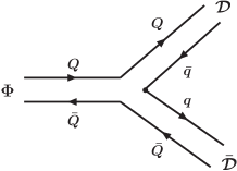
Figure 2: Coupling of the heavy quarkonium $\Phi$ to its decay channel ${\cal D}\bar{\cal D}$.

It is hard to study the $\Phi$-${\cal D}$-$\bar{\cal D}$ vertex shown in FIG. 2 from the first principles of QCD since it is an interaction vertex between three bound states. There are various models describing coupled-channel effects, and the two well accepted models are the Cornell coupled-channel model Cornell ; CCCM and the UQM UQM mentioned in Sec. III. The $\Phi$-${\cal D}$-$\bar{\cal D}$ vertex in the UQM is taken to be the ${}^{3}P_{0}$ quark-pair-creation (QPC) mechanism QPC , i.e., the creation of light quark pair $q\bar{q}$ is supposed to have the vacuum quantum numbers $J^{PC}=0^{++}$ (${}^{3}P_{0}$), and the vertex in FIG. 2 is described by the ${}^{3}P_{0}$ sector of the overlapping integral between the three bound-state wave functions with an almost universal coupling constant $\gamma_{QPC}\approx 3.03$ QPC . The parameters in the UQM are carefully adjusted so that the model gives good fit to the $c\bar{c}$ and $b\bar{b}$ spectra, leptonic widths, etc. It has been shown that the QPC model even also gives not bad results for OZI-allowed productions of light mesons QPC ; QPCappl , which will be relevant in the calculation of the hadronic transition amplitudes in FIG. 3(e) and 3(f) in the coupled-channel theory. So we take the UQM in this section.

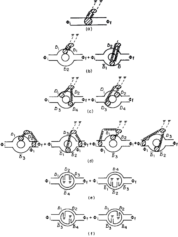
Figure 3: Diagrams for hadronic transitions in the coupled-channel approach. (e) and (f) are new transitions mechanisms beyond the QCD multipole expansion. Quoted from Ref. ZK91 .

In the UQM, the whole Hilbert space is divided into two sectors: namely, the confined sector $|\Phi_{0};\lambda\rangle$ labelled by the discrete quantum number $\lambda$ (say $\sigma$, $n$, $L$, $J$) and the continuous sector $|{\cal D}\bar{\cal D};\nu\rangle$ labelled by the continuous quantum number $\nu$ (say the momentum). The state $|\Phi_{0};\lambda\rangle$ is just the eigenstate of the Hamiltonian $H_{0}$ in the naive single-channel theory with the eigenvalue $M^{0}_{\lambda}$ (the bare mass); i.e.,

$$H_{0}~{}|\Phi_{0};\lambda\rangle=M^{0}_{\lambda}~{}|\Phi_{0};\lambda\rangle,$$ (62)

and the state $|{\cal D}\bar{\cal D};\nu\rangle$ is a state with two freely moving mesons ${\cal D}$ and $\bar{\cal D}$, which is the eigenstate of the kinetic-energy Hamiltonian $H^{c}_{0}$ with the energy eigenvalue $E_{\nu}$; i.e.,

$$H^{c}_{0}|{\cal D}\bar{{\cal D}};\nu\rangle=E_{\nu}|{\cal D}\bar{{\cal D}};\nu\rangle.$$ (63)

The total Hamiltonian $H$ of the system contains $H_{0}$, $H^{c}_{0}$ and the quark-pair-creation Hamiltonian $H_{QPC}$ which determines the OZI-allowed $\Phi$-${\cal D}$-$\bar{\cal D}$ vertex and mixes the two sectors. $H$ can be written as

$$H=\pmatrix{H_{0}~{}~{}~{}~{}0\cr 0~{}~{}~{}~{}H^{c}_{0}}+\pmatrix{~{}~{}~{}0~{}~{}~{}~{}H_{QPC}^{\dagger}\cr H_{QPC}~{}~{}~{}~{}0~{}~{}~{}},$$ (64)

where the first and second rows stand for the confined channel and the continuous channel, respectively. Note that

$$\langle\Phi_{0};\lambda|H_{QPC}|\Phi_{0};\lambda^{\prime}\rangle=0,~{}~{}~{}~{}~{}~{}~{}~{}\langle{\cal D}\bar{\cal D};\nu|H_{QPC}|{\cal D}\bar{\cal D};\nu^{\prime}\rangle=0.$$ (65)

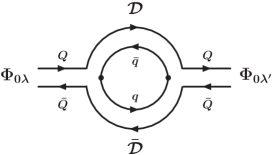
Figure 4: The self-energy $\Pi_{\lambda\lambda^{\prime}}$ from the ${\cal D}$ meson loop.

With $H_{QPC}$ introduced, there will be a self-energy $\Pi_{\lambda\lambda^{\prime}}$ of the quarkonium $\Phi_{0}$ contributed by virtual loops of ${\cal D}$ mesons. This is shown in FIG. 4. The self-energy $\Pi_{\lambda\lambda^{\prime}}$ is not necessarily diagonal, i.e., $\lambda$ and $\lambda^{\prime}$ may be different. This causes the state mixings. For states below the threshold, the self-energy $\Pi_{\lambda\lambda^{\prime}}$ is

$$\Pi_{\lambda\lambda^{\prime}}=-\int\frac{\langle\Phi_{0};\lambda|H_{QPC}|{\cal D}\bar{\cal D};\nu\rangle\langle{\cal D}\bar{\cal D};\nu|H_{QPC}|\Phi_{0};\lambda^{\prime}\rangle}{M_{\lambda}-E_{\nu}}~{}d\nu.$$ (66)

Now the total mass matrix of the quarkonium state is

$$M_{\lambda\lambda^{\prime}}=M^{0}_{\lambda}\delta_{\lambda\lambda^{\prime}}+\Pi_{\lambda\lambda^{\prime}}.$$ (67)

Let $\alpha_{\lambda\lambda^{\prime}}$ be the matrix diagonalizing $M_{\lambda\lambda^{\prime}}$, and $M_{\lambda}$ be the diagonal matrix element. The physical quarkonium state $|\Phi;\lambda\rangle$ is the eigenstate of $H$ with the energy eigenvalue $M_{\lambda}$; i.e.,

$$H~{}|\Phi;\lambda\rangle=M_{\lambda}~{}|\Phi;\lambda\rangle.$$ (68)

The eigenstate $|\Phi;\lambda\rangle$ can be expressed as a superposition of $|\Phi_{0};\lambda\rangle$ and $|{\cal D}\bar{\cal D};\nu\rangle$:

$$|\Phi;\lambda\rangle=\sum_{\lambda}a_{\lambda\lambda^{\prime}}|\Phi_{0};\lambda^{\prime}\rangle+\int c_{\lambda}(\nu)|{\cal D}\bar{\cal D};\nu\rangle~{}d\nu,$$ (69)

in which all possible open heavy flavor mesons ${\cal D}$ ($\bar{\cal D}$) composed of the heavy quark $Q$ and all possible light quarks $\bar{q}$ ($q$) should be included.

The state mixing coefficient $a_{\lambda\lambda^{\prime}}$ is related to $\alpha_{\lambda\lambda^{\prime}}$ by UQM

$$a_{\lambda\lambda^{\prime}}=N_{\lambda}\alpha^{T}_{\lambda\lambda^{\prime}},$$ (70)

where UQM

$$\displaystyle N_{\lambda}=\left[1+\int\left|\frac{\langle{\cal D}\bar{\cal D};\nu|H_{QPC}|\Phi_{0};\lambda\rangle}{M_{\lambda}-E_{\nu}}\right|^{2}d\nu\right]^{-1/2}$$ (71)

is a normalization coefficient, and $N_{\lambda}^{2}$ determines the probability of finding the confined sector $|\Phi_{0};\lambda\rangle$ in the physical state $|\Phi;\lambda\rangle$. The calculation of $\alpha$’s and $N_{\lambda}$’s is tedious, and the results for various $c\bar{c}$ and $b\bar{b}$ states are given in Ref. UQM . The mixing coefficient $c_{\lambda}(\nu)$ is related to $a_{\lambda\lambda^{\prime}}$ by UQM

$$c_{\lambda}(\nu)=\sum_{\lambda^{\prime}}a_{\lambda\lambda^{\prime}}\langle{\cal D}\bar{\cal D};\nu|H_{QPC}|\Phi_{0};\lambda^{\prime}\rangle/(M_{\lambda}-E_{\nu}).$$ (72)

In the single-channel approach, the energy eigenvalues $M^{0}_{\lambda}$ of high lying quarkonium states predicted by potential models are usually higher than the experimental values. In the coupled-channel theory, the self-energy $\Pi_{\lambda\lambda^{\prime}}$ usually causes $M_{\lambda}<M^{0}_{\lambda}$. Since coupled-channel corrections $M_{\lambda}-M^{0}_{\lambda}$ are unimportant for states lying much lower than the ${\cal D}\bar{{\cal D}}$ threshold but are relatively important for states close and above the ${\cal D}\bar{{\cal D}}$ threshold, coupled-channel theory does improve the prediction for the energy spectra. The UQM coupled-channel theory has been applied to obtain successful results of heavy quarkonium spectra, leptonic widths, etc., for the $c\bar{c}$ and $b\bar{b}$ systems UQM .

The formulation of the theory of hadronic transitions in the framework of the UQM was given in Ref. ZK91 . Let $H_{pair}\equiv H_{QPC}+H^{\dagger}_{QPC}$, $\hat{H}_{0}\equiv H_{0}$ for the confining sector and $\hat{H}_{0}\equiv H^{c}_{0}$ for the continuous sector. In the framework of UQM, the $S$ matrix element (15) becomes ZK91

$$\langle F|S|I\rangle = -i2\pi\delta(E_{F}+\omega_{f}-E_{I})\bigg{<}F~{}\bigg{|}(H_{2}+H_{pair})\frac{1}{E_{I}-\hat{H}_{0}+i\partial_{0}-H_{1}}(H_{2}+H_{pair})\cdots$$ (73)

$$\times(H_{2}+H_{pair})\frac{1}{E_{I}-\hat{H}_{0}+i\partial_{0}-H_{1}}(H_{2}+H_{pair})\bigg{|}~{}I\bigg{>},$$

For isospin-conserving $\pi\pi$ transitions (dominated by E1E1 gluon emissions), we take the electric dipole term in $H_{2}$ [cf. Eq. (11)]. Note that, in Eq. (73), the creation of the two pions can come not only from the conversion of the two emitted gluons (OZI-forbidden mechanism) via the two $H_{2}$’s, but also from the OZI-allowed mechanism $\langle{\cal D}\bar{\cal D}\pi;\nu|H_{QPC}|{\cal D}\bar{\cal D};\nu\rangle$ directly from the light quark lines [cf. FIG. 3(e)-3(f)]. Note that the two gluons can only convert into two pions (not one pion) due to isospin conservation. Thus these two pion creation mechanisms contribute separately. The $\pi\pi$ transition $S$ matrix element between two physical quarkonium states $|\Phi;\lambda_{I}\rangle$ and $|\Phi;\lambda_{F}\rangle$ is ZK91

$$\langle\Phi;\lambda_{F};\pi({\bm{k}}_{1})\pi({\bm{k}}_{2})|S|\Phi;\lambda_{I}\rangle=-i2\pi\delta(M_{f}+E_{\pi_{1}}+E_{\pi_{2}}-M_{I})\sum_{\lambda^{\prime}_{i}\lambda^{\prime}_{f}}a_{\lambda_{I}\lambda^{\prime}_{i}}a_{\lambda_{F}\lambda^{\prime}_{f}}\bigg{<}\Phi_{0};\lambda^{\prime}_{f};\pi({\bm{k}}_{1})\pi({\bm{k}}_{2})\bigg{|}$$

$$\hskip 17.07182pt\times\bigg{[}H_{2}\frac{1}{M_{I}-\hat{H}_{0}+i\partial_{0}-H_{1}}H_{2}+H^{\dagger}_{QPC}\frac{1}{M_{I}-\hat{H}_{0}+i\partial_{0}-H_{1}}H_{2}\frac{1}{M_{I}-\hat{H}_{0}+i\partial_{0}-H_{1}}H_{2}\frac{1}{M_{I}-\hat{H}_{0}}H_{QPC}$$

$$\hskip 17.07182pt+H_{2}\frac{1}{M_{I}-\hat{H}_{0}+i\partial_{0}-H_{1}}H^{\dagger}_{QPC}\frac{1}{M_{I}-\hat{H}_{0}+i\partial_{0}-H_{1}}H_{2}\frac{1}{M_{I}-\hat{H}_{0}}H_{QPC}$$

$$\hskip 17.07182pt+H^{\dagger}_{QPC}\frac{1}{M_{I}-\hat{H}_{0}+i\partial_{0}-H_{1}}H_{2}\frac{1}{M_{I}-\hat{H}_{0}+i\partial_{0}-H_{1}}H_{QPC}\frac{1}{M_{I}-\hat{H}_{0}+i\partial_{0}-H_{1}}H_{2}$$

$$\hskip 17.07182pt+H^{\dagger}_{QPC}\frac{1}{M_{I}-\hat{H}_{0}}H_{QPC}\frac{1}{M_{I}-\hat{H}_{0}}H_{QPC}\frac{1}{M_{I}-\hat{H}_{0}}H_{QPC}\bigg{]}\bigg{|}\Phi_{0};\lambda^{\prime}_{i}\bigg{>},$$ (74)

where $E_{\pi_{1}}$ and $E_{\pi_{2}}$ are energies of the two pions. The Feynman diagrams corresponding to the terms in (74) are shown in FIG. 3 in whic FIG. 3(a)$\--$Fig. 3(d) are diagrams corresponding to the first four terms in (74), and FIG. 3(e)$\--$FIG. 3(f) are diagrams for the last term in (74). For convenience, we shall call the first four terms in (74) the MGE part, and call the last term in (74) the quark-pair-creation (QPC) part.

We see that (74) contains much more channels of $\pi\pi$ transitions than the single-channel theory does. In the MGE part, FIG. 3(a) is similar to FIG. 1 but with state mixings, so that the single-channel amplitude mentioned in Sec. IIIA is only a part of the first term in (74). In the QPC part, the last term in (74) is a new pion creation mechanism through $H_{QPC}$ irrelevant to MGE. Thus in the coupled-channel theory, $\pi\pi$ transitions between heavy quarkonium states are not merely described by QCDME.

Since the state mixings and the QPC vertices depending on the bound-state wave functions are all different in the $c\bar{c}$ and the $b\bar{b}$ systems, the predictions for $\Gamma(\Upsilon^{\prime}\to\Upsilon~{}\pi\pi)$, $\Gamma(\Upsilon^{\prime\prime}\to\Upsilon~{}\pi\pi)$ and $\Gamma(\Upsilon^{\prime\prime}\to\Upsilon^{\prime}~{}\pi\pi)$ by taking $\Gamma_{expt}(\psi^{\prime}\to J/\psi~{}\pi\pi)$ as input will be different from those in the single-channel theory. Such predictions were studied in Ref. ZK91 in which the same potential model as in Ref. UQM is taken for avoiding the tedious calculation of $\alpha$’s and $N_{\lambda}$’s. Note that for a given QPC model, the QPC part in (74) is fixed, while the MGE part still contains an unknown parameter $C_{1}$ in its hadronization factor after taking the approximation (36). Since there is interference between the MGE part and the QPC part, the phase of $C_{1}$ will affect the result. Let

$$C_{1}=|C_{1}|~{}\displaystyle e^{i\vartheta}.$$ (75)

Two input data are thus needed to determine $|C_{1}|$ and $\vartheta$. In Ref. ZK91 , the data of the transition rate and $M_{\pi\pi}$ distribution in $\psi^{\prime}\to J/\psi~{}\pi\pi$ are taken as the inputs. Considering the experimental errors in the $M_{\pi\pi}$ distribution, $\vartheta$ is restricted in the range  $-1\leq\cos\vartheta\leq-0.676$. The details of the calculation are given in Ref. ZK91 in which the ${\cal D}$ meson states $D~{}(B)$, $D^{*}~{}(B^{*})$, and $D^{**}~{}(B^{**})$ are taken into account. The so predicted transition rates $\Gamma(\Upsilon^{\prime}\to\Upsilon~{}\pi\pi)$, $\Gamma(\Upsilon^{\prime\prime}\to\Upsilon~{}\pi\pi)$, and $\Gamma(\Upsilon^{\prime\prime}\to\Upsilon^{\prime}~{}\pi\pi)$ for $\cos\vartheta=-1$ and $\cos\vartheta=-0.676$ are listed in TABLE IV together with the updated experimental results for comparison.

Table 4: The predicted rates $\Gamma(\Upsilon^{\prime}\to\Upsilon~{}\pi\pi)$, $\Gamma(\Upsilon^{\prime\prime}\to\Upsilon~{}\pi\pi)$, and $\Gamma(\Upsilon^{\prime\prime}\to\Upsilon^{\prime}~{}\pi\pi)$ ( in keV) in the coupled-channel theory with $\cos\vartheta=-1$ and $\cos\vartheta=-0.676$. The corresponding updated experimental values of the transition rates quoted from Ref. PDG are also listed for comparison.

		Theory		Expt.
	$\cos\vartheta=-1$		$\cos\vartheta=-0.676$
$\Gamma(\Upsilon^{\prime}\to\Upsilon~{}\pi\pi)$ (keV)	14		13	$~{}~{}~{}12.0~{}\pm 1.8~{}~{}~{}~{}~{}~{}$
$\Gamma(\Upsilon^{\prime\prime}\to\Upsilon~{}\pi\pi)$ (keV)	1.1		1.0	$1.72\pm 0.35$
$\Gamma(\Upsilon^{\prime\prime}\to\Upsilon^{\prime}~{}\pi\pi)$ (keV)	0.1		0.3	$1.26\pm 0.40$

We see that the obtained $\Gamma(\Upsilon^{\prime}\to\Upsilon~{}\pi\pi)$ is in good agreement with the experiment, and the results of $\Gamma(\Upsilon^{\prime\prime}\to\Upsilon~{}\pi\pi)$ and $\Gamma(\Upsilon^{\prime\prime}\to\Upsilon^{\prime}~{}\pi\pi)$ are in agreement with the experiments at the level of $2\sigma$ and $2.4\sigma$, respectively.

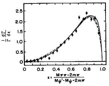
Figure 5: Comparison of the coupled-channel theory predicted curve of $d\Gamma(\Upsilon^{\prime}\to\Upsilon~{}\pi\pi)/dM_{\pi\pi}$ with the ARGUS data ARGUS . The solid and dashed-dotted lines stand for $\cos\theta=-1$ and $\cos\theta=-0.676$, respectively. The dashed line is the naive single-channel result for comparison. Quoted from Ref. ZK91 .

Next we look at the predicted $M_{\pi\pi}$ distributions. It is pointed out in Ref. ARGUS that there is a tiny difference between the the measured $M_{\pi\pi}$ distributions in $\psi^{\prime}\to J/\psi~{}\pi\pi$ and $\Upsilon^{\prime}\to\Upsilon~{}\pi\pi$. In the single-channel theory, the formulas for these $M_{\pi\pi}$ distributions are the same with the same value of $|C_{1}|$. Ref. ARGUS tried to explain the tiny difference by taking the approach to the H factor given in Ref. VZNS in which there is a parameter $\kappa$ which is supposed to run. However, the running of $\kappa$ is not known theoretically, so that it is not clear whether the running of $\kappa$ from the scale $M_{\psi^{\prime}}-M_{J/\psi}=590$ MeV to the scale $M_{\Upsilon^{\prime}}-M_{\Upsilon}=560$ MeV can really explain the tiny difference or not. Furthermore, as we have seen in Sec. IIIC that the approach given in Ref. VZNS is ruled out by the recent BES and CLEO-c experiments. In the present coupled-channel theory, once the values of $|C_{1}|$ and $\vartheta$ are determined by the input data of $\psi^{\prime}\to J/\psi~{}\pi\pi$, the $M_{\pi\pi}$ distribution of $\Upsilon^{\prime}\to\Upsilon~{}\pi\pi$ is definitely predicted. The comparison of the predicted distribution with the experimental data given in Ref. ARGUS is shown in FIG. 5. We see that the agreement is good, so that the coupled-channel theory successfully predicts the tiny difference.

However, the situation of the $M_{\pi\pi}$ distributions of $\Upsilon^{\prime\prime}\to\Upsilon~{}\pi^{+}\pi^{-}$ and $\Upsilon^{\prime\prime}\to\Upsilon^{\prime}~{}\pi^{+}\pi^{-}$ are more complicated. The single-channel theory predicts $M_{\pi\pi}$ distributions similar to FIG. 5 for these two process, i.e., the distributions are peaked at the large $M_{\pi\pi}$ region. The CLEO data shows a clear double-peaked shape for the $M_{\pi\pi}$ distribution of $\Upsilon^{\prime\prime}\to\Upsilon~{}\pi^{+}\pi^{-}$ [cf. Fig. 6(a)] CLEO87 ; CLEO9491 . The coupled-channel theory does enhance the low-$M_{\pi\pi}$ region a little, but is far from giving a double-peaked shape as is shown by the solid and dashed-dottd curves in FIG. 6(a). Actually, this situation is not only for the coupled-channel theory based on the UQM. The Cornell coupled-channel model is not substantially different from the UQM ZK91 . Compared with the UQM, the Cornell coupled-channel model leads to relatively larger $S-S$ mixings but smaller $S-D$ mixings after taking the same experimental inputs. So that the Cornell coupled-channel model gives even smaller enhancement in the low-$M_{\pi\pi}$ region. Thus the transition $\Upsilon^{\prime\prime}\to\Upsilon~{}\pi^{+}\pi^{-}$ needs further investigations with new ideas although the predicted transition rate $\Gamma(\Upsilon^{\prime\prime}\to\Upsilon~{}\pi^{+}\pi^{-})$ is consistent with the CLEO data at the $2\sigma$ level.

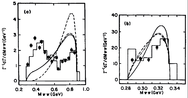
Figure 6: Comparison of the coupled-channel theory predicted curves of $d\Gamma(\Upsilon^{\prime\prime}\to\Upsilon~{}\pi^{+}\pi^{-})/dM_{\pi\pi}$ [FIG. 6(a)] and $d\Gamma(\Upsilon^{\prime\prime}\to\Upsilon^{\prime}~{}\pi^{+}\pi^{-})/dM_{\pi\pi}$ [FIG. 6(b)] with the CLEO data CLEO87 . The solid and dashed-dotted lines stand for $\cos\theta=-1$ and $\cos\theta=-0.676$, respectively. The dashed line is the naive single-channel result for comparison. Quoted from Ref. ZK91 .

There have been various attempts to explain the double-peaked shape. Ref. Voloshin-Truong assumed the existence of a four-quark state $\Upsilon_{1}$ having nearly the same mass as $\Upsilon^{\prime\prime}$ and coupling strongly to $\Upsilon^{\prime\prime}\pi$ and $\Upsilon\pi$, and the dominant transition mechanism is suggested to be $\Upsilon^{\prime\prime}\to\Upsilon_{1}+\pi\to\Upsilon+\pi+\pi$ which enhances the low-$M_{\pi\pi}$ distribution. The branching ratio of $\Upsilon(4S)\to\Upsilon_{1}+\pi$ is estimated to be roughly $1\%$, so that the assumption can be experimentally tested by searching for the $\Upsilon_{1}$ state in $\Upsilon(4S)$ decays. This idea was carefully studied in Ref. BDM taking account of the final-state $\pi\pi$ interactions and got a double-peaked shape but the low-$M_{\pi\pi}$ peak is not at the desired position. A slightly modified model of this kind was proposed in Ref. ABSZ . So far the assumed four-quark state is not found experimentally. Another attempt was made in Ref. Lipkin-Tuan-Moxhay assuming that the coupled-channel contributions are strong enough in $\Upsilon^{\prime\prime}\to\Upsilon~{}\pi\pi$ that there is a considerably large QPC part in the transition amplitude, and the interference between it and the MGE part may form a double-peaked shape by adjusting the strength of the QPC part. However, as we mentioned above that the strength of the QPC part is fixed once a QPC model is given, and the systematic calculation in Ref. ZK91 shows that the QPC part is actually much smaller than what was expected in Ref. Lipkin-Tuan-Moxhay . Recently, attempts to explain the double-peaked shape by certain models for a light $\sigma$ meson resonance at around 500 MeV in the final state $\pi\pi$ interactions with Ishida01 and without Uehara using the Breit-Wigner formula have been proposed. By adjusting the free parameters in the models, the CLEO data on the $M_{\pi\pi}$ distributions in $\Upsilon^{\prime\prime}\to\Upsilon~{}\pi\pi$ and $\Upsilon^{\prime\prime}\to\Upsilon^{\prime}~{}\pi\pi$ can be fitted. However, the models need to be tested in other processes. Therefore, the $\Upsilon^{\prime\prime}\to\Upsilon~{}\pi\pi$ transition is still an interesting process needing further investigations.

We would like to mention that the calculations mentioned above concerns the wave functions of some excited states of heavy quarkonia, the heavy flavored mesons ${\cal D}$, and the pions. Nonrelativistic potential model calculations of these wave functions may not be so good. Therefore the nonrelativistic coupled-channel theory of hadronic transitions in Ref. ZK91 still needs further improvements.

V Application of QCD Multipole Expansion to Radiative Decays of $\bm{J/\psi}$

In the preceding sections, QCD multipole expansion is applied to various hadronic transition processes in which the initial- and final-state quarkonia $\Phi_{I}$ and $\Phi_{F}$ are composed of the same heavy quarks. In this case, the dressed (constituent) quark field $\Psi(\bm{x},t)$ does not actually need to be quantized. Now we generalize the QCDME theory to processes including heavy quark flavor changing and heavy quark pair annihilation or creation. Then the quantization of the $\Psi(\bm{x},t)$ is needed. This has been studied in Ref. KYF , and the obtained canonical commutation relation is KYF

$$[\Psi(\bm{x},t),\Psi^{\dagger}(\bm{x}^{\prime},t)]=\delta^{3}(\bm{x}-\bm{x}^{\prime}).$$ (76)

To include the electromagnetic and weak interactions, we generalize the Hamiltonian as

$$H=H^{(0)}_{QCD}+H_{int},$$ (77)

$$H_{int}=H^{(1)}_{QCD}+H_{em}+H_{W},$$ (78)

in which $H^{(0)}_{QCD}$ and $H^{(1)}_{QCD}$ are defined in Eqs. (9) and (11), and

$$H_{em} = e\int d^{3}x~{}\bar{\Psi}(\bm{x},t)\gamma^{\mu}{\cal Q}{\cal A}_{\mu}(\bm{x},t)\Psi(\bm{x},t),$$

$$H_{W} = \int d^{3}x\bigg{[}\frac{g}{\sqrt{2}}\bar{\Psi}(\bm{x},t)\gamma^{\mu}\frac{1-\gamma_{5}}{2}[t_{+}W^{+}_{\mu}(x)+t_{-}W^{-}_{\mu}(x)]\Psi(\bm{x},t)$$ (79)

$$+\frac{g}{\cos\theta_{W}}\bar{\Psi}(\bm{x},t)\gamma^{\mu}\bigg{(}\frac{1-\gamma_{5}}{2}t_{3}-\sin^{2}\theta_{W}{\cal Q}\bigg{)}Z_{\mu}(x)\Psi(\bm{x},t)\bigg{]},$$

where ${\cal Q}$ is the electric charge operator of the heavy quark, ${\cal A}_{\mu}$ is the photon field, $g$ and $t_{i}$ are, respectively, the weak $SU(2)$ coupling constant and generator, $\theta_{W}$ is the Weinberg angle, and $e=g\sin\theta_{W}$ is the electromagnetic coupling constant.

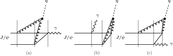
Figure 7: Feynman diagrams for the radiative decay process $J/\psi\to\gamma+\eta$. The intermediate states between two vertical dotted lines are all bound states.

Let us take the application of the generalized theory to the radiative decay process $J/\psi\to\gamma+\eta$ as an example. This process has been studied in the framework of perturbative QCD and nonrelativistic quark model in Ref. KKKS , but the predicted rate is significantly smaller than the experimental value. We know that the momentum of the $\eta$ meson in this process is $q_{\eta}=(M^{2}_{L/\psi}-m^{2}_{\eta})/(2M_{J/\psi})=1.5$ GeV. Suppose the $\eta$ meson is converted from two emitted gluons from the heavy quark. The typical momentum of a gluon is then $k\sim q_{\eta}/2\sim 750$ MeV. This is the momentum scale that perturbative QCD does not work well but QCDME works KYF . So we can calculated the rate of this decay process using QCDME. The Feynman diagrams for this process are shown in FIG. 7, in which the intermediate states marked between two vertical dotted lines are all treated as bound states in this approach. In this sense this approach is nonperturbative, and also for this reason the contributions of the three diagrams in FIG. 7 are different.

In QCDME, this process is dominated by the E1M2 gluon emissions. So the H factor (conversion of the two gluons into $\eta$) is

$$g_{E}g_{M}\langle\eta|E^{a}_{j}D_{j}B^{a}_{i}|0\rangle,$$ (80)

where $D_{j}\equiv\partial_{j}-g_{s}(\lambda_{a}/2)A^{a}_{j}$ is the covariant derivative. The operator in (80) can be written as

$$E^{a}_{j}D_{j}B^{a}_{i}=\partial_{j}(E^{a}_{j}B^{a}_{i})-(D_{j}E^{a}_{j})B^{a}_{i}.$$

It is argued in Ref. VZNS that the second term is smaller than the first term, so they suggested the approximation

$$g_{E}g_{M}\langle\eta|E^{a}_{j}D_{j}B^{a}_{i}|0\rangle\simeq iq_{\eta j}\langle\eta|E^{a}_{j}B^{a}_{i}|0\rangle.$$ (81)

This matrix element can then be evaluated by using the Gross-Treiman-Wilczeck formula GTW and we obtain KYF

$$g_{E}g_{M}\langle\eta|E^{a}_{j}D_{j}B^{a}_{i}|0\rangle\simeq i\frac{g_{E}g_{M}}{g_{s}^{2}}\frac{4\pi^{2}}{3\sqrt{6}}q_{\eta i}f_{\pi}m_{\eta}^{2}(\cos\theta_{P}-\sqrt{2}\sin\theta_{P})\delta_{ij},$$ (82)

where $\theta_{P}$ is the mixing angle in the pseudoscalar nonet, i.e.,

$$\eta=\eta_{8}\cos\theta_{P}-\eta_{1}\sin\theta_{P},~{}~{}~{}~{}~{}~{}\eta^{\prime}=\eta_{8}\sin\theta_{P}+\eta_{1}\cos\theta_{P},$$ (83)

with

$$\eta_{8}=\frac{1}{\sqrt{6}}(\bar{u}\gamma_{5}u+\bar{d}\gamma_{5}d-2\bar{s}\gamma_{5}s),~{}~{}~{}~{}\eta_{1}=\frac{1}{\sqrt{3}}(\bar{u}\gamma_{5}u+\bar{d}\gamma_{5}d+\bar{s}\gamma_{5}s).$$ (84)

As in Sec. IIID, we take $\alpha_{s}\simeq\alpha_{E}=0.6$. It is shown in Ref. KYF that the contribution of FIG. 7(a) is larger than those of FIG. 7(b) and FIG. 7(c). Thus as an approximation, we only consider the main contribution of FIG. 7(a).

The calculated $~{}J/\psi\to\gamma\eta~{}$ rate is KYF

$$\Gamma(J/\psi\to\gamma\eta)=\frac{1}{6\pi}\bigg{(}\frac{\alpha_{M}}{\alpha_{E}}\bigg{)}\frac{|\bm{q}_{\eta}|^{3}}{M_{J/\psi}}\bigg{(}\frac{2e{\cal Q}}{3\sqrt{6}m_{c}}\bigg{)}^{2}\bigg{[}\frac{4\pi^{2}}{3\sqrt{6}}f_{\pi}m_{\eta}^{2}(\cos\theta_{P}-\sqrt{2}\sin\theta_{P})\sum_{n}h^{111}_{10n0}\bigg{]}^{2},$$ (85)

where

$$h^{LP_{i}P}_{n_{I}l_{i}nl}\equiv\sum_{K}\frac{\langle R_{n_{F}}|r^{P}|R^{\prime}_{KL}\rangle\langle R^{\prime}_{KL}|r^{P_{i}}|R_{n_{I}l_{i}}\rangle}{(M_{J/\psi}-E_{nl}-\omega_{\eta})(M_{J/\psi}-E^{\prime}_{KL})}f_{nl}(0),$$ (86)

in which $R_{n_{I}l_{i}}$, $R_{nl}$ and $R^{\prime}_{KL}$ are radial wave functions of the initial-, final-, and intermediate-quarkonium states in FIG. 7(a), respectively. $f_{nl}(0)$ is the wave function at the origin of the final-quarkonium state. We shall take into account the first five terms in the summation $\displaystyle\sum_{n}h^{111}_{10n0}$. As is well-known that $f_{n0}(0)$ can be determined by the datum of the related leptonic width $\Gamma(\psi(n^{3}S_{1})\to e^{+}e^{-})$. For $n=1,2$, the so determined $f_{10}(0)$ and $f_{20}(0)$ are smaller than the ones predicted by the Cornell potential model by almost the same factor 0.57 Cornell . It is expected that this discrepancy may be explained by QCD corrections. For $n\geq 3$, the states are above the threshold and state mixings will be significant, so that the data of $\Gamma(\psi(n^{3}S_{1})\to e^{+}e^{-})$ are not useful. We expect that QCD corrections will not vary seriously with $n$ as is inspired by the cases of $n=1,2$. Then we can calculate $f_{10}(0),\cdots f_{50}(0)$ using the Cornell potential model, and then multiply the obtained results by the same factor 0.57 to obtain the correct values of them.

The factor $(\cos\theta_{P}-\sqrt{2}\sin\theta_{P})$ in (82) concerns the effective $\eta$-$g$-$g$ vertex in the hadronization $gg\to\eta$. This is somewhat similar to the effective $\eta$-$\gamma$-$\gamma$ vertex in $\eta\to\gamma\gamma$. We may take the determined value of $\theta_{P}$ from the $\eta\to\gamma\gamma$ and $\eta^{\prime}\to\gamma\gamma$ data, which is $\theta_{P}\approx-20^{\circ}$ PDG . With this value of $\theta_{P}$, we get

$$\Gamma(J/\psi\to\gamma\eta)=0.041\bigg{(}\frac{\alpha_{M}}{\alpha_{E}}\bigg{)}~{}{\rm keV}.$$ (87)

With the experimental datum $\Gamma_{tot}(J/\psi)=91.0\pm 3.2$ keV PDG , we obtain

$$B(J/\psi\to\gamma\eta)=(4.5\pm 0.2)\times 10^{-4}\bigg{(}\frac{\alpha_{M}}{\alpha_{E}}\bigg{)}.$$ (88)

The experimental value of this branching ratio is PDG

$$B(J/\psi\to\gamma\eta)\bigg{|}_{expt}=(8.6\pm 0.8)\times 10^{-4}.$$

We see that for $\alpha_{M}/\alpha_{E}\approx 1.9$, the predicted branching ratio agrees with the experimental value.

Note that the value of $\alpha_{M}/\alpha_{E}$ and $\theta_{P}$ are not so certain, and we do not know how good the approximation (81) really is. To avoid these uncertainties, we can take the ratio of $\Gamma(J/\psi\to\gamma\eta)$ to another E1M2 transition rate $\Gamma(\psi^{\prime}\to J/\psi\eta)$. The theoretical prediction is KYF

$$R_{\eta}\equiv\frac{\Gamma(J/\psi\to\gamma\eta)}{\Gamma(\psi^{\prime}\to J/\psi\eta)}=\frac{\displaystyle\frac{8}{81}(e{\cal Q})^{2}|\bm{q}_{\eta}(J/\psi\to\gamma\eta)|^{3}/M_{J/\psi}\bigg{|}\displaystyle\sum_{n}h^{111}_{10n0}\bigg{|}^{2}}{\frac{2}{243}|\bm{q}_{\eta}(\psi^{\prime}\to J/\psi\eta)|^{3}|f^{111}_{2010}|^{2}}=0.012.$$ (89)

In this ratio, the uncertainties mentioned above are all cancelled, so that $R_{\eta}$ just tests the MGE mechanism in this approach. The corresponding experimental value is PDG

$$R_{\eta}\bigg{|}_{expt}=0.009\pm 0.003.$$ (90)

We see that the agreement is at the $1\sigma$ level. Since we have seen in Sec. IIID that the calculation of the MGE factor mentioned in Sec. III is quite reasonable, the agreement of (89) with (90) implies that MGE mechanism for this radiative decay process is also reasonable.

The above approach can also be applied to the radiative decay process $J/\psi\to\gamma\eta^{\prime}$. From (83) we see that the $J/\psi\to\gamma\eta^{\prime}$ decay rate is

$$\Gamma(J/\psi\to\gamma\eta^{\prime})=\frac{1}{6\pi}\bigg{(}\frac{\alpha_{M}}{\alpha_{E}}\bigg{)}\frac{|\bm{q}_{\eta^{\prime}}|^{3}}{M_{J/\psi}}\bigg{(}\frac{2e{\cal Q}}{3\sqrt{6}m_{c}}\bigg{)}^{2}\bigg{[}\frac{4\pi^{2}}{3\sqrt{6}}f_{\pi}m_{\eta^{\prime}}^{2}(\sqrt{2}\cos\theta_{P}+\sin\theta_{P})\sum_{n}h^{111}_{10n0}\bigg{]}^{2},$$ (91)

Since there is no $\psi^{\prime}\to J/\psi\eta^{\prime}$ available (not enough phase space), we cannot have a ratio similar to $R_{\eta}$ which exactly tests the MGE mechanism. We can define the ratio

$$R_{\eta^{\prime}}\equiv\frac{\Gamma(J/\psi\to\gamma\eta^{\prime})}{\Gamma(\psi^{\prime}\to J/\psi\eta)}=\bigg{|}\frac{{\bf q}(J/\psi\to\gamma\eta^{\prime})}{{\bf q}(J/\psi\to\gamma\eta))}\bigg{|}^{3}\bigg{|}\frac{m_{\eta^{\prime}}^{2}(\sqrt{2}\cos\theta_{P}+\sin\theta_{P})}{m_{\eta}^{2}(\cos\theta_{P}-\sqrt{2}\sin\theta_{P})}\bigg{|}^{2}R_{\eta}.$$ (92)

Taking $\theta_{P}\approx-20^{\circ}$ determined from the $\eta\to\gamma\gamma$ and $\eta^{\prime}\to\gamma\gamma$ rates, we predict

$$R_{\eta^{\prime}}=0.044.$$ (93)

The corresponding experimental value of $R_{\eta^{\prime}}$ is PDG

$$R_{\eta^{\prime}}\bigg{|}_{expt}=0.044\pm 0.010.$$ (94)

We see that this prediction is also in agreement with the experiment.

It has been shown in Ref. KYF that the contribution of the above mechanism to the isospin violating radiative decay $J/\psi\to\gamma+\pi^{0}$ is negligibly small. There is another important mechanism giving the main contribution to $J/\psi\to\gamma+\pi^{0}$. It is the $\rho^{0}$ meson dominance mechanism $J/\psi\to\rho^{0*}+\pi^{0}\to\gamma+\pi^{0}$. This has been studied in Ref. FJ , and the result is close to the experimental value .

We would like to mention that this approach is not suitable for $\Upsilon\to\gamma\eta$ since the typical gluon momentum in this process is $k\sim q_{\eta}/2\sim 2.4$ GeV at which perturbative QCD works, while QCD multipole expansion does not. Studies of the processes $\Upsilon\to\gamma\eta$, $\Upsilon\to\gamma\eta^{\prime}$ and $\Upsilon\to\gamma f_{2}(1270)$ have been carried out in Ref. Ma . Application of this approach to $\psi^{\prime}\to\gamma\eta$ is more complicated since both relativistic and coupled-channel corrections are important in this process. Thus developing a relativistic coupled-channel is desired.

QCDME can also be applied to study the direct photon spectrum in $J/\psi\to\gamma+{\rm hadrons}~{}$ near $x\simeq 1$, where $x\equiv 2\omega_{\gamma}/M$ with $\omega_{\gamma}$ the energy of the photon and $M$ the mass of the quarkonium. Conventional study of the process $J/\psi(\Upsilon)\to\gamma+{\rm hadrons}$  are based on perturbative QCD calculation of  $J/\psi(\Upsilon)\to\gamma+g+g$  in the Born approximation BDHC . The direct photon spectrum is expressed as

$$\frac{1}{\Gamma_{tot}}\frac{d\Gamma(J/\psi(\Upsilon)\to\gamma+{\rm hadrons})}{dx}.$$

For $\Upsilon$, the obtained result is in good agreement with the experiment CUSB ; Photiadis ; Field , while for $J/\psi$ the obtained distribution is too hard, i.e., in the range $x>0.8$, the obtained distribution is much larger than the experimental values Scharre . In $J/\psi\to\gamma+{\rm hadrons}$, the typical gluon momentum at $x\simeq 1$ is $k\simeq 770$ MeV, so that we can apply QCDME to it for $x\geq 0.9$. The calculation was done in Ref. CCKY , and the obtained direct photon spectrum for $x\geq 0.9$ is very close to the experimental values CCKY . For $x<0.9$, the typical gluon momentum is too large for QCDME to work. A successful theory for the whole range of $x$ is still expected.

VI Summary and Outlook

In this paper, we have reviewed the theory and applications of QCDME. We see from Secs. III$\--$V that nonrelativistic QCDME theory gives many successful predictions for hadronic transition and some radiative decay rates in heavy quarkonium systems. Even the simple nonrelativistic single-channel theory can work well for many processes. Although the single-channel approach gives too small rates for $\Upsilon^{\prime}\to\Upsilon\pi\pi$, $\Upsilon^{\prime\prime}\to\Upsilon\pi\pi$, and $\Upsilon^{\prime\prime}\to\Upsilon^{\prime}\pi\pi$ (cf. TABLE I), nonrelativistic coupled-channel theory improves the prediction (cf. TABLE IV). We summarize the above mentioned main successful predictions for the transition and decay rates in TABLE V together with the corresponding experimental results for comparison.

Table 5: Summary of the predictions for transition and decay rates in the nonrelativistic QCD multipole expansion approach together with the corresponding experimental results for comparison.

	Theoretical predictions	Experimental data	Places in the text
$\Gamma(\Upsilon^{\prime}\to\Upsilon~{}\pi\pi)$	13 keV	$12.0\pm 1.8$ keV (PDG)	TABLE IV
$\Gamma(\Upsilon^{\prime\prime}\to\Upsilon~{}\pi\pi)$	1.0 keV	$1.72\pm 0.35$ keV (PDG)	TABLE IV
$\Gamma(\Upsilon^{\prime\prime}\to\Upsilon^{\prime}~{}\pi\pi)$	0.3 keV	$1.26\pm 0.40$ keV (PDG)	TABLE IV
$\Gamma(\Upsilon^{\prime}\to\Upsilon~{}\eta)$	0.022 keV	$<0.086$ keV (PDG)	Eqs.(29)(30)
$\Gamma(\Upsilon^{\prime\prime}\to\Upsilon~{}\eta)$	0.011 keV	$<0.058$ keV (PDG)	Eqs.(29)(30)
$\displaystyle R^{\prime}\equiv\frac{\left|f^{111}_{2010}(b\bar{b})/m_{b}\right|^{2}|\bm{q}(b\bar{b})|^{3}}{\left|f^{111}_{2010}(c\bar{c})/m_{c}\right|^{2}|\bm{q}(c\bar{c})|^{3}}$	0.0025	$<0.0098$ (BES, PDG)	Eqs.(32)(31)
$\displaystyle R^{\prime\prime}\equiv\frac{\left|f^{111}_{3010}(b\bar{b})/m_{b}\right|^{2}|\bm{q}(b\bar{b})|^{3}}{\left|f^{111}_{2010}(c\bar{c})/m_{c}\right|^{2}|\bm{q}(c\bar{c})|^{3}}$	0.0013	$<0.0065$ (BES, PDG)	Eqs.(32)(31)
$\Gamma\big{(}\chi_{b}(2^{3}P_{0})\to\chi_{b}(1^{3}P_{0})~{}\pi\pi\big{)}$	0.4 keV	$\--$	TABLE II
$\Gamma\big{(}\chi_{b}(2^{3}P_{0})\to\chi_{b}(1^{3}P_{2})~{}\pi\pi\big{)}$	$0.002\--0.02$ keV	$\--$	TABLE II
$\Gamma\big{(}\chi_{b}(2^{3}P_{1})\to\chi_{b}(1^{3}P_{1})~{}\pi\pi\big{)}$	0.4 keV	$(0.83\pm 0.22\pm 0.08\pm 0.19)$ keV	TABLE II
$\Gamma\big{(}\chi_{b}(2^{3}P_{1})\to\chi_{b}(1^{3}P_{2})~{}\pi\pi\big{)}$	$0.001\--0.01$ keV	$\--$	TABLE II
$\Gamma\big{(}\chi_{b}(2^{3}P_{2})\to\chi_{b}(1^{3}P_{2})~{}\pi\pi\big{)}$	0.4 keV	$(0.83\pm 0.22\pm 0.08\pm 0.19)$ keV	TABLE II
$\Gamma\big{(}\psi(3770)\to J/\psi~{}\pi^{+}\pi^{-}\big{)}$	$(32\--147)$ keV	$(80\pm 32\pm 21)$ keV (BES)	TABLE III,Eq.(45)
		$(50.5\pm 16.9)$ keV (CLEO-c)	Eq.(48)
$B(\psi^{\prime}\to h_{c}\pi^{0})B(h_{c}\to\eta_{c}\gamma)$	$(1.9\--5.8)\times 10^{-4}$	$(4\pm 0.8\pm 0.7)\times 10^{-4}$ (CLEO-c)	Eqs.(59)(60)
$R_{\eta}\equiv\Gamma(J\psi\to\gamma\eta)/\Gamma(\psi^{\prime}\to J/\psi~{}\eta)$	0.012	$0.009\pm 0.003$	Eqs.(89)(90)
$R_{\eta^{\prime}}\equiv\Gamma(J\psi\to\gamma\eta^{\prime})/\Gamma(\psi^{\prime}\to J/\psi~{}\eta)$	0.044	$0.044\pm 0.010$	Eqs.(92)(94)

In addition, the prediction for the $M_{\pi\pi}$ distribution in $\Upsilon^{\prime}\to\Upsilon\pi\pi$ from the nonrelativistic coupled-channel theory is in good agreement with the data (cf. FIG. 5).

However, despite of the above success, there are experimental results which this simple nonrelativistic approach cannot explain. CLEO experiment shows a clear double-peak shape for the $M_{\pi\pi}$ distribution in $\Upsilon^{\prime\prime}\to\Upsilon~{}\pi\pi$ [cf. FIG. 6(a)]. Nonrelativistic coupled-channel correction is so small that it cannot account for this shape. Whether this double-peak shape can be explained by the final state $\pi\pi$ interactions or it is caused by other physical effects is still not clear yet. Further investigation is needed.

Another problem is that, in the nonrelativistic single-channel approach, the $S$-wave to $S$-wave transitions rates are contributed only by the $C_{1}$ term in Eq. (19) due to the orbital angular momentum selection rule, i.e., the obtained $\pi\pi$ angular correlation is isotropic in the laboratory frame. However, experiments on $\psi^{\prime}\to J/\psi~{}\pi\pi$ BES01 shows a small angular dependence (a $0.2\%$ ingredient of $D$-wave) of the $\pi\pi$ angular correlation which cannot be explained by the nonrelativistic single-channel theory . Theoretically, the angular dependence of the transition rates may come from: (a) coupled-channel corrections [state-mixing leads to the $C_{2}$ term ($D$-wave) contributions], and (b) relativistic corrections [orbital angular momentum no longer conserves in the relativistic theory]. Actually, the sizes of the corrections (a) and (b) are of the same order of magnitude, and there is interference between them. Therefore to obtain a theoretical prediction for the $\pi\pi$ angular correlation, both (a) and (b) corrections should be taken into account. This means that a systematic relativistic coupled-channel theory of hadronic transitions is expected. So far there is still no such a theory due to the difficulty of dealing with the two-body bound-state equation in relativistic quantum mechanics. There have been various attempts to solve the relativistic two-body problem. Making effort on developing a systematic relativistic coupled-channel theory of hadronic transition is really important.

In a word the nonrelativistic theory of QCDME approach is not the end of the story. Further development is needed.

Acknowledgment

This work is supported by National Natural Science Foundation of China under Grant No. 90403017.

References

- (1) K. Gottfried, in Proc. 1977 International Symposium on Lepton and Photon Interactions at High Energies, edited by F. Gutbrod, DESY, Hamburg, 1977, p. 667; Phys. Rev. Lett. 40 (1978) 598.
- (2) G. Bhanot, W. Fischler and S. Rudas, Nucl. Phys. B 155 (1979) 208.
- (3) M.E. Peskin, Nucl. Phys. B 156 (1979) 365; G. Bhanot and M.E. Peskin, ibid. 156 (1979) 391.
- (4) M.B. Voloshin, Nucl. phys. B 154 (1979) 365; M.B. Voloshin and V.I. Zakharov, Phys. Rev. Lett. 45 (1980) 688; V.A. Novikov and m.A. Shifman, Z. Phys. C 8 (1981) 43.
- (5) T.M. Yan, Phys. Rev. D 22 (1980) 1652.
- (6) Y.-P. Kuang, Y.-P. Yi and B. Fu, Phys. Rev. D 42 (1990) 2300.
- (7) Y.-P. Kuang and T.-M. Yan, Phys. Rev. D 24 (1981) 2874.
- (8) S.-H. H. Tye, Phys. Rev. D 13 (1976) 3416; R.C. Giles and S.-H. H. Tye, Phys. Rev. Lett. 37 (1976) 1175; Phys. Rev. D 16 (1977) 1079; W. Buchmüller and S.-H. H. Tye, Phys. Rev. Lett. 44 (1980) 850.
- (9) D.-S. Liu and Y.-P. Kuang, Z. Phys. C 37 (1987) 119; P.-Z. Bi and Y.-M. Shi, Mod. Phys. Lett. A 7 (1992) 3161.
- (10) L.S. Brown and R.N. Cahn, Phys. Rev. Lett. 35 (1975) 1.
- (11) S. Eidelman et al. (Particle Data Group), Review of Particle physics, Phys. Lett. B 592 (2004) 1.
- (12) E. Eichten, K. Gottfried, T. Kinoshita, K.D. Lane, and T.-M. Yan, Phys. Rev. D 17 (1978) 3090; ibid., D 21 (1980) 203.
- (13) W. Buchmüller, G. Grunberg, and S.-H. H. Tye, Phys. Rev. Lett. 45 (1980) 103; W. Buchmüller and S.-H. H. Tye, Phys. Rev. D 24 (1981) 132.
- (14) Y.-P. Kuang, S.F. Tuan, and T.-M. Yan, Phys. Rev. D 37 (1998) 1210.
- (15) J.Z. Bai et al. (BES Collaboration), Phys. Rev. D 70 (2004) 012006.
- (16) T. Skwarnicki, talk presented at the 40th Rencontres De Moriond on QCD and High Energy Hadronic Interactions, 12-19 March 2005, La Thuile, Aosta Valley, Italy, hep-ex/0505050.
- (17) C. Cawlflield et al. (CLEO Collaboration), hep-ex/0511019.
- (18) R.A. Partridge, Ph.D. thesis, Report No. CALT-68-1150, 1984.
- (19) R.H. Schindler, Ph.D. thesis, Report No. SLAC-219, UC-34d(T/E),1979.
- (20) J. Adler, et al., Phys. Rev. Lett. 60 (1988) 89.
- (21) A. Billoire, R. Lacaze, A. Morel, and H. Navelet, Nucl. Phys. B155 (1979) 493.
- (22) P. Moxhay, Phys. Rev. D 37 (1988) 2557; P. Ko, Phys. Rev. D 47 (1993) 208.
- (23) Y.-P. Kuang and T.-M. Yan, Phys. Rev. D 41 (1990) 155.
- (24) Y.-P. Kuang, Phys Rev. D 65 (2002) 094024.
- (25) S. Godfrey, Z. Phys. C 31 (1986) 77.
- (26) K. Heikkilä, S. Ono, and N.A. Törnqvist, Phys. Rev. D 29 (1984) 110; 29 (1984) 2136(E); S. Ono and N.A. Törnqvist, Z. Phys. C 23 (1984) 59; N.A. Törnqvist, Phys. Rev. Lett. 53 (1984) 878; Acta Phys. Pol. B 16 (1985) 503.
- (27) Y.-Q. Chen and Y.-P. Kuang, Phys. Rev. D 46 (1992) 1165; 47 (1993) 350(E).
- (28) J.Z. Bai et al. (BES Collaboration), Phys. Lett. B 605 (2005) 63.
- (29) N.E. Adam et al. (CLEO Collaboration), hep-ex/0508023.
- (30) G. Bonvicini et al. (CLEO collaboration), Phys. Rev. D 70 (2004) 032001.
- (31) T.A. Armstrong et al., Phys. Rev. Lett. 69 (1992) 2337.
- (32) C. Patrignani, Nucl. Phys. Proc. Suppl., 142 (2005) 98.
- (33) Crystal Ball Group, Annu. Rev. Nucl. Part. Sci. 33 (1983) 143.
- (34) D.J. Gross, S.B. Treiman, and F. Wilczeck, Phys. Rev. D 19 (1979) 2188.
- (35) P. Rubin et al (CLEO Collaboration), Phys. Rev. D 72 (2005) 092004, hep-ex/0508037; J.L. Rosner et al. (CLEO Collabration), Phys. Rev. Lett. 95 (2005) 102003.
- (36) For example, Ref. Cornell and V.E. Zambetakis, Ph.D. thesis, University of California Report No. UCLA/86/TEP/2.
- (37) A. Le Yaouanc, L. Oliver, O. Pene, and J.-C. Raynal, Phys. Rev. D 8 (1973) 2223.
- (38) M. Chaichian and R. Kögerler, Ann. Phys. (N.Y.) 124 (1980) 61.
- (39) H.-Y. Zhou and Y.-P. Kuang, Phys. Rev. D 44 (1991) 756.
- (40) H. Albrecht et al., Z. Phys. C 35 (1987) 283.
- (41) J. Green et al. (CLEO Collabration), Phys. Rev. Lett. 49 (1982) 617; T. Bowcock et al. (CLEO Collabration), ibid. 58 (1987) 307.
- (42) F. Butler et al. (CLEO Collaboration), Phys. Rev. D 49 (1994) 40; C. Bebek et al. (CLEO Collaboration), ibid., D 43 (1991) 1448.
- (43) M.B. Voloshin, Pis’ma Zh. Eksp. Teor. Fiz. 37 (1983) 58 (JETP Lett. 37 (1983) 69); T.N. Truong, Univeristy of Virginia report (unpublished).
- (44) G. Bélinger, T. DeGrand, and P. Moxhay, Phys. Rev. D 39 (1989) 257.
- (45) V.V. Anisovich, D.V. Bugg, A.V. Saratsev, and B.S. Zou, Phys. Rev. D 51 (1995) R4619.
- (46) H.J. Lipkin and S.F. Tuan, Phys. Lett. B 206 (1988) 349; P. Moxhay, Phys. Rev. D 39 (1989) 3497.
- (47) T. Komada, M. Ishida, and S. Ishida, Phys. Lett. B 508 (2001) 31; M. Ishida, S. Ishida, T. Komada, and S.-I. Matsumoto, ibid., B 518 (2001) 47.
- (48) M. Uehara, Prog. Theor. Phys. 109 (2003) 265.
- (49) J.G. Köner, J.H. Kühn, M Krammer, and H. Schneider, nucl. Phys. B 229 (1983) 115.
- (50) J.P. Ma, Phys. Rev. D 65 (2002) 097506; Nucl. Phys B 605 (2001) 625.
- (51) S. J. Brodsky, T.A. DeGrand, R.R. Horgan, and D.G. Coyne, phys. Lett. 73B (1978) 203.
- (52) R.D. Schamberger et al. (CUSB Collaboration), Phys. Lett. 138B (1984) 225; S.E. Csorna et al. (CLEO Collaboration), Phys. Rev. Lett. 56 (19860 1222; H. Albrecht et al. (ARGUS Collaboration), Phys. Lett. B 199 (1987) 291.
- (53) D.M. Photiadis, Phys. Lett. 164B (1985) 160.
- (54) R.D. Field, Phys. Lett. 133B (1983) 248.
- (55) D.L. Scharre et al., Phys. Rev. D 23 (1981) 43. See also K. Königsmann, Phys. Rep. 139C (1986) 243; K. Köpke and N. Wermes, ibid. 174C (1989) 67.
- (56) C.-H. Chang, G.-P. Chen, Y.-P. Kuang, and Y.-P. Yi, Phys. Rev. D 42 (1990) 2309.
- (57) J.Z. Bai et al. (BES Collaboration), Phys. Rev. D 62 (2000) 032002.
- (58) H. Fritzsch and J.D. Jackson, Phys. Lett. 66B (1977) 265.