High Momentum Dilepton Production from Jets in a Quark Gluon Plasma

Abstract

We discuss the emission of high momentum lepton pairs in central Au+Au collisions at RHIC ($\sqrt{s_{NN}}=$200 GeV) and Pb+Pb collisions at the LHC ($\sqrt{s_{NN}}=$5500 GeV). Yields of dileptons produced through interactions of jets with thermal partons have been calculated, with next-to-leading order corrections through hard thermal loop (HTL) resummation. They are compared to thermal dilepton emission and the Drell-Yan process. A complete leading order treatment of jet energy loss has been included. Jet-plasma interactions are found to dominate over thermal dilepton emission for all values of the invariant mass $M$. Drell-Yan is the dominant source of high momentum lepton pairs for $M>$ 3 GeV at RHIC, after the background from heavy quark decays is subtracted. At LHC, the range $M<7$ GeV is dominated by jet-plasma interactions. Effects from jet energy loss on jet-plasma interactions turn out to be weak, but non-negligible, reducing the yield of low-mass dileptons by about $30\%$.

I Introduction

Finding experimental evidence for the existence of a Quark-Gluon Plasma (QGP) is one of the main reasons for conducting relativistic heavy ion collisions. In this context, real and virtual photons can be used to probe the high temperature and density phase in these collisions: due to their large mean free path, electromagnetic radiation suffers only little final state interactions Feinb:76 ; Shuryak:1978ij . More recently, photons emitted from jets interacting with the medium have been suggested as a further signature prlphoton . A quantitative characterization of the different sources contributing to the photon yield in high energy heavy ion collisions can be found in simon2 . In this work, we concentrate on virtual photons decaying into lepton pairs.

Several sources for lepton pairs compete and have to be considered: dileptons from the Drell-Yan process drell-yan , thermal dileptons kkmm both from the QGP kms ; altherr and from the subsequent hadronic phase gale_lichard ; rapp_wam , dileptons from the absorption of jets by the plasma prcdilep and dileptons from bremsstrahlung of jets. Besides the thermal emission, dileptons from the latter two sources carry information about the medium. Comparing with the baseline $p+p$ process, we note that absorption of jets exclusively happens in nucleus-nucleus collisions in the presence of a medium. There is a also a significant change in bremsstrahlung emission expected in a medium (in A+A) compared to the case of vacuum (in $p+p$).

The main background for dileptons are correlated charm decays ($D\bar{D}\rightarrow e^{+}e^{-}X$) at intermediate mass Shor:1989yt , while one has to cope with Dalitz decays of light mesons ($\pi^{0}\rightarrow\gamma e^{+}e^{-},\omega\rightarrow\pi^{0}e^{+}e^{-}$) at low mass $M\leq$ 1 GeV. In principle, there is also another source of dileptons corresponding to pre-equilibrium emission. It is difficult to assess both theoretically and experimentally, nevertheless, such calculations have been attempted geiger .

In Ref. prcdilep the dilepton yield from the passage of jets through a plasma has been evaluated as a function of invariant mass at leading order. The results show that this process dominates over thermally induced reactions at high invariant mass $M$. However, energy loss of jets in the medium has not been included in this calculation. Large energy loss of jets was discovered as one of the most exciting results from the Relativistic Heavy Ion Collider (RHIC) and has been observed in the suppression of high $p_{T}$ hadron spectra phenix2 ; star and through the disappearance of back-to-back correlations of high $p_{T}$ hadrons star2 .

In this paper we re-examine the leading order dilepton production from jets note1 and we explore the effect of energy loss. We assume here that jets lose their energy by induced gluon bremsstrahlung only Gyu_plum ; wgp . We use the approach developed by Arnold, Moore, and Yaffe (AMY) AMY , which correctly treats the Landau-Pomeranchuk-Migdal (LPM) effect (up to $O(g_{s})$ corrections) migdal . This model has been used successfully to reproduce the measured nuclear modification factor $R_{AA}$ of neutral pions, the ratio of all photons over background photons and the direct photon yield at RHIC simon2 . Jets will be defined by all partons produced initially with transverse momentum $p_{T}^{\rm jet}\gg 1$ GeV. The total dilepton production could be influenced by the choice of the cutoff $p_{T}^{\rm jet}$. As we will discuss below, in order to avoid such sensitivity, we limit our study to high momentum dileptons.

In perturbation theory at high temperature, it is important to distinguish between hard momenta, on the order of the temperature $T$, and soft momenta, on the order of $g_{s}T$, where the QCD coupling constant is assumed to be small, $g_{s}\ll 1$. Only at the end of the calculations, will the results be extrapolated to more realistic value of the coupling constant. When a line entering a vertex is soft, there are an infinite number of diagrams with loop corrections contributing to the same order in the coupling constant as the tree amplitude. These corrections can be treated with the hard thermal loop (HTL) resummation technique developed in Ref. htl . This technique has been used thereafter in Refs. braaten_dil ; Wong:1991be ; thoma to show that the production rate of low mass dileptons ($M<T$) could differ from the Born-term quark-antiquark annihilation by orders of magnitude. In this work, we apply this technique to go beyond the leading order jet-medium interaction.

The dilepton production rate in finite-temperature field theory is calculated in Sec. II and the physical processes underlying each contribution are discussed in Sec. III in the framework of relativistic kinetic theory. In Sec. IV, we include these dilepton production rates in a model for a longitudinally expanding QGP fireball. In Sec. V we calculate the yield from the Drell-Yan process and correlated leptons from heavy quark decays. The numerical results are presented in Sec. VI. Finally, Sec. VII contains our summary and conclusions.

II Dilepton Production Rate from Finite-Temperature Field Theory

Within the thermal field theory framework, the production rate of a lepton pair with momenta $p_{+}$ and $p_{-}$ is given by vmd91

$$E_{+}E_{-}\frac{dR^{e^{+}e^{-}}}{d^{3}p_{+}d^{3}p_{-}}=\frac{2e^{2}}{(2\pi)^{6}(p_{+}+p_{-})^{4}}(p_{+}^{\mu}p_{-}^{\nu}+p_{-}^{\mu}p_{+}^{\nu}-g^{\mu\nu}p_{+}\cdot p_{-})\frac{{\rm Im}\Pi^{R}_{\mu\nu}}{e^{(E_{+}+E_{-})/T}-1}$$ (1)

where $\Pi^{R}_{\mu\nu}$ is the finite-temperature retarded photon self-energy. After integration over the angular distribution of the lepton pair, we get

$$\frac{dR^{e^{+}e^{-}}}{d^{4}p}=2E\frac{dR^{e^{+}e^{-}}}{dM^{2}d^{3}p}=\frac{2\alpha}{3\pi M^{2}}E\frac{dR^{\gamma^{*}}}{d^{3}p}=\frac{\alpha}{12\pi^{4}M^{2}}\frac{{\rm Im}\Pi^{R\mu}_{\mu}}{1-e^{E/T}}$$ (2)

where $\vec{p}=\vec{p_{+}}+\vec{p_{-}},E$ and $M$ are the momentum, energy and invariant mass of the virtual photon.

In the HTL formalism, the leading order resummed photon self-energy diagram is shown in the left hand side of Fig. 1. The heavy dots indicate a resummed propagator or vertex. The second diagram in Fig. 1, coming from the effective two-photon-two quark vertex, is needed in order to fulfill the Ward identity

$$p^{\mu}\Pi^{R}_{\mu\nu}(p)=0.$$ (3)

Using power counting htl ; lebellac , the HTL resummation gives corrections of order $g_{s}^{2}T^{2}/|\vec{p}|^{2}$ to each bare vertex of the first diagram of Fig. 1, while the bare propagators receive $g_{s}^{2}T^{2}/|\vec{q}-\vec{p}|^{2}$ and $g_{s}^{2}T^{2}/|\vec{q}|^{2}$ corrections. A resummed propagator consists of an infinite number of gluon correction, as shown in Fig. 2.

In this work, we are interested in the high momentum dilepton limit ($|\vec{p}|\gg T$), so that vertex corrections can be neglected, and at least one propagator is guaranteed to be hard. We assume that this is the propagator associated with momentum $q-p$. Then the propagator associated with $q$ can be soft or hard, implying that is has to be resummed. Also, for the high $|\vec{p}|$ limit, the second diagram of Fig. 1 gives only $g_{s}^{2}T^{2}/|\vec{p}|^{2}$ corrections to the first diagram. The resulting diagram that has to be evaluated is shown in Fig. 3 and its contribution to the self-energy is

$$\Pi^{\mu}_{\mu}(p)=3e^{2}\sum_{f}\left(\frac{e_{f}}{e}\right)^{2}T\sum_{n}\int\frac{d^{3}q}{(2\pi)^{3}}\mbox{Tr}\left[\gamma^{\mu}S_{D}(q)\gamma_{\mu}S(q-p)\right]$$ (4)

with the sum running over the Matsubara frequencies. The diagram in Fig. 3 includes the leading order effect, and some next-to leading order corrections in $g_{s}$. In order to have a complete next-to leading order production rate in the region $|\overrightarrow{p}|\gg T$, contributions like bremsstrahlung need to be included. This will be discussed in the last section.

The dressed fermion propagator, in Euclidean space ($\not\!q=-iq_{0}\gamma^{0}+\vec{q}\cdot\hat{\gamma}$), is given by kapusta_book

$$S_{D}(q)=\frac{1}{\not\!q+\Sigma}=\frac{\gamma^{0}-\hat{\gamma}\cdot\hat{\bf q}}{2D_{+}(q)}+\frac{\gamma^{0}+\hat{\gamma}\cdot\hat{\bf q}}{2D_{-}(q)}$$ (5)

where

$$D_{\pm}(q)=-iq_{0}\pm|\overrightarrow{q}|+A\pm B$$ (6)

The terms $A$ and $B$ describe the quark self-energy

$$\Sigma=A\gamma^{0}+B\hat{\gamma}\cdot\hat{\bf q}.$$ (7)

In the HTL approximation, one obtains lebellac

$$A=\frac{m_{F}^{2}}{|\vec{q}|}Q_{0}\left(\frac{iq_{0}}{|\vec{q}|}\right),\quad B=-\frac{m_{F}^{2}}{|\vec{q}|}Q_{1}\left(\frac{iq_{0}}{|\vec{q}|}\right)$$ (8)

where $m_{F}=g_{s}T/\sqrt{6}$ is the effective quark mass induced by the thermal medium and the $Q_{n}$ are Legendre functions of the second kind. The bare propagator $S(q)$ is the same as $S_{D}(q)$, with $D_{\pm}$ replaced by

$$d_{\pm}(q)=-iq_{0}\pm|\vec{q}|$$ (9)

Using those expressions for the quark propagators and carrying out the trace, Eq. 4 leads to

$$\Pi^{\mu}_{\mu}(p) = 6e^{2}\sum_{f}\left(\frac{e_{f}}{e}\right)^{2}T\sum_{n}\int\frac{d^{3}q}{(2\pi)^{3}}$$ (10)

$$\times\Big{[}\frac{1}{D_{+}(q)}\left(\frac{1-\hat{\bf q}\cdot\hat{\bf k}}{d_{+}(k)}+\frac{1+\hat{\bf q}\cdot\hat{\bf k}}{d_{-}(k)}\right)+\frac{1}{D_{-}(q)}\left(\frac{1+\hat{\bf q}\cdot\hat{\bf k}}{d_{+}(k)}+\frac{1-\hat{\bf q}\cdot\hat{\bf k}}{d_{-}(k)}\right)\Big{]}$$

where we have defined $k=q-p$.

Figure 1: Resummed photon self-energy diagrams.

Figure 2: Resummed quark propagator.

Figure 3: Effective photon self-energy diagram for hard external momentum $p$.

At this point it is convenient to introduce the spectral representation of the effective quark propagator defined by

$$\rho_{\pm}(\omega,\left|\vec{q}\right|) = -2\mbox{Im}\,\frac{1}{D_{\pm}(iq_{0},\left|\vec{q}\right|)},$$

$$\frac{1}{D_{\pm}(iq_{0},\left|\vec{q}\right|)} = \int_{-\infty}^{\infty}\frac{d\omega}{2\pi}\frac{\rho_{\pm}(\omega,\left|\vec{q}\right|)}{iq_{0}-\omega+i\epsilon}.$$ (11)

This implies

$$\rho_{\pm}(\omega,\left|\vec{q}\right|)= - 2\pi\frac{\omega^{2}-\left|\vec{q}\right|^{2}}{2m_{F}^{2}}\left[\delta\left(\omega-\omega_{\pm}(\left|\vec{q}\right|)\right)+\delta\left(\omega+\omega_{\mp}(\left|\vec{q}\right|)\right)\right]-2\pi\beta_{\pm}\left(\omega,\left|\vec{q}\right|\right)\Theta\left(\left|\vec{q}\right|^{2}-\omega^{2}\right)$$ (12)

with

$$\beta_{\pm}(\omega,\left|\vec{q}\right|)=\frac{\frac{m_{F}^{2}}{2\left|\vec{q}\right|}(1\mp\omega/\left|\vec{q}\right|)}{\left[-\omega\pm\left|\vec{q}\right|+\frac{m_{F}^{2}}{\left|\vec{q}\right|}\left(\pm 1+\frac{1}{2}\ln\left|\frac{\omega+\left|\vec{q}\right|}{\omega-\left|\vec{q}\right|}\right|\right)(1\mp\omega/\left|\vec{q}\right|)\right]^{2}+\left(\frac{\pi m_{F}^{2}}{2\left|\vec{q}\right|}(1\mp\omega/\left|\vec{q}\right|)\right)^{2}}\,.$$ (13)

Here $\omega_{\pm}=\omega_{\pm}(\left|\vec{q}\right|)$ correspond to the poles of the effective quark propagator. They are solution of $D_{\pm}(\omega,\left|\vec{q}\right|)=0$. The solution $\omega=\omega_{+}$ represents an ordinary quark with an effective thermal mass $\sqrt{2}m_{F}$ and a positive helicity over chirality ratio, $\chi=1$ braaten_dil . The solution $\omega=\omega_{-}$ represents a particle having negative helicity over chirality ratio, $\chi=-1$. This collective mode, called plasmino, has no analog at zero temperature. Following the notation of Ref. braaten_dil , we denote the ordinary modes by $q_{+}$ and the plasminos by $q_{-}$. The spectral density of the bare propagator is simply

$$r_{\pm}(\omega^{\prime},|\vec{k}|) = -2\mbox{Im}\,\frac{1}{d_{\pm}(ik_{0},|\vec{k}|)}=-2\pi\delta(\omega^{\prime}\mp|\vec{k}|)$$ (14)

Using the spectral density representation has the advantage that one can carry out the sum over Matsubara frequencies with help of the elegant identity braaten_dil ,

$$\mbox{Im}\,T\sum_{n}F_{1}(iq_{0})F_{2}(iq_{0}-ip_{0}) = \pi\left(1-e^{E/T}\right)\int_{-\infty}^{\infty}\frac{d\omega}{2\pi}\int_{-\infty}^{\infty}\frac{d\omega^{\prime}}{2\pi}$$ (15)

$$\times\rho_{1}(\omega)\rho_{2}(-\omega^{\prime})\delta(E-\omega-\omega^{\prime})f_{\mathrm{FD}}(\omega)f_{\mathrm{FD}}(\omega^{\prime})$$

where $f_{\mathrm{FD}}$ is the Fermi-Dirac phase space distribution function and $\rho_{i}$ is the spectral density associated with $F_{i}$. We use the analytical continuation $ip_{0}\rightarrow E+i\epsilon$ with the dilepton energy $E$.

Putting all information together, we obtain

$${\rm Im}\,\Pi^{R\mu}_{\mu} = -6e^{2}\pi\sum_{f}\left(\frac{e_{f}}{e}\right)^{2}\left(1-e^{E/T}\right)\int\frac{d^{3}q}{(2\pi)^{3}}\int_{-\infty}^{\infty}\frac{d\omega}{2\pi}f_{\mathrm{FD}}(\omega)$$ (16)

$$\times\Big{[}\rho_{+}(\omega,\left|\vec{p}\right|)\Big{\{}\delta(E-\omega+E_{1})(1-\hat{\bf q}\cdot\hat{\bf k})f_{\mathrm{FD}}(-E_{1})+\delta(E-\omega-E_{1})(1+\hat{\bf q}\cdot\hat{\bf k})f_{\mathrm{FD}}(E_{1})\Big{\}}$$

$$\quad+\rho_{-}(\omega,\left|\vec{p}\right|)\Big{\{}\delta(E-\omega+E_{1})(1+\hat{\bf q}\cdot\hat{\bf k})f_{\mathrm{FD}}(-E_{1})+\delta(E-\omega-E_{1})(1-\hat{\bf q}\cdot\hat{\bf k})f_{\mathrm{FD}}(E_{1})\Big{\}}\Big{]}$$

with $E_{1}=\left|\vec{q}-\vec{p}\right|$. Since both $E\gg T$ and $E_{1}\gg T$, the terms proportional to $\delta(E-\omega+E_{1})$ are exponentially suppressed by the factor $f_{\mathrm{FD}}(\omega)$ for $\omega\gg T$. Also, because $E_{1}$ corresponds to a massless parton, energy and momentum conservation does not permit the terms containing $\delta(E+|\omega|-E_{1})$ for $\omega^{2}>\left|\vec{q}\right|^{2}$, i.e. there is no phase space available for the process $1\to 2+3$ if parton $1$ is on-shell. These arguments lead to further simplifications and we have

$${\rm Im}\,\Pi^{R\mu}_{\mu} = 6e^{2}\pi\sum_{f}\left(\frac{e_{f}}{e}\right)^{2}\left(1-e^{E/T}\right)\int\frac{d^{3}q}{(2\pi)^{3}}$$ (17)

$$\times\Big{[}f_{\mathrm{FD}}(\omega_{+})f_{\mathrm{FD}}(E_{1})\frac{\omega_{+}^{2}-\left|\vec{q}\right|^{2}}{2m_{F}^{2}}\delta(E-\omega_{+}-E_{1})(1+\hat{\bf q}\cdot\hat{\bf k})$$

$$\quad+f_{\mathrm{FD}}(\omega_{-})f_{\mathrm{FD}}(E_{1})\frac{\omega_{-}^{2}-\left|\vec{q}\right|^{2}}{2m_{F}^{2}}\delta(E-\omega_{-}-E_{1})(1-\hat{\bf q}\cdot\hat{\bf k})$$

$$\quad+\int_{-\infty}^{\infty}d\omega f_{\mathrm{FD}}(\omega)f_{\mathrm{FD}}(E_{1})\Big{\{}\beta_{+}(\omega,\left|\vec{q}\right|)(1+\hat{\bf q}\cdot\hat{\bf k})+\beta_{-}(\omega,\left|\vec{q}\right|)(1-\hat{\bf q}\cdot\hat{\bf k})\Big{\}}\delta(E-\omega-E_{1})\Big{]}.$$

Now we analyze the integral over $d^{3}q=\left|\vec{q}\right|^{2}d\left|\vec{q}\right|d\Omega$. When $\left|\vec{q}\right|$ becomes as large as $E_{1}$, the propagator associated with $q$ does not have to be resummed. If $\left|\vec{q}\right|$ gets much bigger, implying $E_{1}\sim g_{s}T$, then this is the propagator associated with $E_{1}$ which should be resummed. We have a symmetry relatively to the point $\left|\vec{q}\right|=E_{1}$, such that $\int_{0}^{\infty}d\left|\vec{q}\right|\rightarrow\int_{0}^{\infty}d\left|\vec{q}\right|2\Theta(E_{1}-\left|\vec{q}\right|)$. According to Eq. (2) the dilepton production rate is thus given by

$$\frac{dR^{e^{+}e^{-}}}{d^{4}p} = \frac{2\alpha^{2}}{\pi^{2}M^{2}}\sum_{f}\left(\frac{e_{f}}{e}\right)^{2}\int_{0}^{\infty}2\left|\vec{q}\right|^{2}d\left|\vec{q}\right|\int\frac{d\Omega}{(2\pi)^{3}}$$ (18)

$$\times\Big{[}f_{\mathrm{FD}}(\omega_{+})f_{\mathrm{FD}}(E_{1})\frac{\omega_{+}^{2}-\left|\vec{q}\right|^{2}}{2m_{F}^{2}}\delta(E-\omega_{+}-E_{1})(1-\hat{\bf q}\cdot\hat{\bf p}_{1})\Theta(E_{1}-\left|\vec{q}\right|)$$

$$\quad+f_{\mathrm{FD}}(\omega_{-})f_{\mathrm{FD}}(E_{1})\frac{\omega_{-}^{2}-\left|\vec{q}\right|^{2}}{2m_{F}^{2}}\delta(E-\omega_{-}-E_{1})(1+\hat{\bf q}\cdot\hat{\bf p}_{1})\Theta(E_{1}-\left|\vec{q}\right|)$$

$$\quad+\int_{-\infty}^{\infty}d\omega f_{\mathrm{FD}}(\omega)f_{\mathrm{FD}}(E_{1})\delta(E-\omega-E_{1})\Theta(E_{1}-\left|\vec{q}\right|)$$

$$\qquad\times\Big{\{}\beta_{+}(\omega,\left|\vec{q}\right|)(1-\hat{\bf q}\cdot\hat{\bf p}_{1})+\beta_{-}(\omega,\left|\vec{q}\right|)(1+\hat{\bf q}\cdot\hat{\bf p}_{1})\Big{\}}\Big{]}$$

where $\hat{\bf p}_{1}=\vec{p}_{1}/|\vec{p}_{1}|=-\hat{\bf k}$.

The dilepton production rate from finite-temperature field theory calculated in this section follows the path presented in Refs. KLS91 ; thoma . New to our approach is that we keep the general form of the function $f_{FD}(E_{1})$ until the end of the calculation, while this function is integrated out and information about it is finally lost, in the earlier work. In the next section we will analyze, for the first time, the physical processes behind the production rate in relativistic kinetic theory. This is done so that $f_{\mathrm{FD}}(E_{1})$ can be interpreted as the phase-space distribution function of an incoming parton of energy $E_{1}$. Once this is established one can apply the usual technique and obtain the production rate involving jets by substituting the thermal distribution $f_{\mathrm{FD}}(E_{1})$ by the time-dependent jet distribution $f_{\mathrm{jet}}(E_{1},t)$.

Figure 4: Processes extracted from photon self-energy in Fig. 3. In the picture, the particle with energy $E_{1}$ is an anti-quark, but the quark contribution is also included in the calculation.

III Dilepton Production Rate from Relativistic Kinetic Theory

We will show in this section that the production rate in Eq. (18) can also be interpreted in relativistic kinetic theory. Indeed, after cutting the diagram in Fig. 3, we get the Feynman amplitudes shown in Fig. 4. The process in Fig. 4(a) corresponds to the annihilation of the hard antiquark of energy $E_{1}$ with a soft quasiparticle $q_{+}$ or $q_{-}$. This is the pole-pole contribution, as it involves the propagation of the poles of the propagator in the diagram shown in Fig. 3. Fig. 4(b) corresponds to Compton scattering of an antiquark with energy $E_{1}$ with a hard gluon from the medium, with the exchange of a soft quasiparticle and Fig. 4(c) represents the annihilation of an antiquark $E_{1}$ with a hard quark from the medium with the exchange of a soft quasiparticle. They correspond to a cut through the self-energy of the dressed propagator in Fig. 3: this is thus called the cut-pole contribution. There is no $s$-channel process because hard thermal loops have imaginary parts for $q^{2}<0$ only lebellac . The dots mean that the quasiparticle propagator is resummed. That modification of the propagator in the space-like region at non-zero temperature is known as Landau damping.

The production rate, as computed from relativistic kinetic theory (kt), for reaction $1+2\rightarrow\gamma^{*}+3+...$ is

$$E\frac{dR^{\gamma^{*}}_{\mbox{kt}}}{d^{3}p}=\int\left(\prod_{i}\frac{d^{3}p_{i}}{2(2\pi)^{3}E_{i}}\right)(2\pi)^{4}\delta^{4}(p_{1}+p_{2}-p-p_{3}-...)\left|{\cal M}\right|^{2}\frac{f(E_{1})f(E_{2})(1\pm f(E_{3}))...}{2(2\pi)^{3}}$$ (19)

where ${\cal M}$ is the invariant scattering matrix element.

III.1 Pole-Pole Contributions ($1+q_{\pm}\rightarrow\gamma^{*}$)

The production rate for the process of Fig. 4(a) is

$$E\frac{dR^{\gamma^{*}}_{\mbox{kt}a}}{d^{3}p} = \int\frac{d^{3}p_{1}}{2(2\pi)^{3}E_{1}}\frac{d^{3}q}{2(2\pi)^{3}q_{0}}(2\pi)^{4}\delta^{4}(p_{1}+q-p)\left|{\cal M}_{\mbox{kt}a}\right|^{2}\frac{f^{q+\bar{q}}(E_{1})f_{\mathrm{FD}}(q_{0})}{2(2\pi)^{3}}$$ (20)

$$= \int\frac{d^{3}q}{8(2\pi)^{5}q_{0}E_{1}}\delta(E_{1}+q0-E)\left|{\cal M}_{\mbox{kt}a}\right|^{2}f^{q+\bar{q}}(E_{1})f_{\mathrm{FD}}(q_{0})$$

where $f^{q+\bar{q}}(E_{1})$ is the phase-space distribution of quarks and antiquarks with energy $E_{1}$. The square of the matrix element, after summation over spin and color is

$$\left|{\cal M}_{\mbox{kt}a}\right|^{2} = \left|{\cal M}_{1+q_{+}\rightarrow\gamma^{*}}\right|^{2}+\left|{\cal M}_{1+q_{-}\rightarrow\gamma^{*}}\right|^{2}$$ (21)

$$= 6e^{2}\sum_{f}\left(\frac{e_{f}}{e}\right)^{2}\mbox{Tr}\left[\not\!p_{1}\left(\sum_{s}u_{s}^{q_{+}}(q)\bar{u}_{s}^{q_{+}}(q)+\sum_{s}u_{s}^{q_{-}}(q)\bar{u}_{s}^{q_{-}}(q)\right)\right]$$

We need to find a completeness relation for $\sum_{s}u_{s}^{q_{\pm}}(q)\bar{u}_{s}^{q_{\pm}}(q)$. The dressed propagator in Minkowski space is

$$-iS_{D}(q)=\frac{1}{\not\!q-\Sigma}=-\frac{\gamma^{0}-\hat{\gamma}\cdot\hat{\bf q}}{2D_{+}(q)}-\frac{\gamma^{0}+\hat{\gamma}\cdot\hat{\bf q}}{2D_{-}(q)}$$ (22)

and by definition, it is peskin

$$-iS_{D}(q)=\frac{\sum_{s}u_{s}^{q_{+}}(q)\bar{u}_{s}^{q_{+}}(q)}{q^{2}-m_{q_{+}}^{2}}+\frac{\sum_{s}u_{s}^{q_{-}}(q)\bar{u}_{s}^{q_{-}}(q)}{q^{2}-m_{q_{-}}^{2}}$$ (23)

where $m_{+}$ and $m_{-}$ are the physical mass of the quasiparticles. We expand $D_{\pm}$ around the pole located at $q_{0}=\omega_{\pm}$:

$$D_{\pm}(q) \approx (q_{0}-\omega_{\pm})\frac{\partial D_{\pm}}{\partial q_{0}}\Big{|}_{q_{0}=\omega_{\pm}}=(q_{0}-\omega_{\pm})\left(-1+\frac{\partial}{\partial q_{0}}(A\pm B)\right)\Big{|}_{q_{0}=\omega_{\pm}}$$ (24)

$$= -\frac{m_{F}^{2}(q^{2}-m_{\pm}^{2})}{(\omega_{\pm}^{2}-|\vec{q}|^{2})\omega_{\pm}}$$

From Eqs. (22), (23) and (24), we finally obtain the relation

$$\sum_{s}u_{s}^{q_{\pm}}(q)\bar{u}_{s}^{q_{\pm}}(q)=\frac{\omega_{\pm}(\omega_{\pm}^{2}-|\vec{q}|^{2})}{2m_{F}^{2}}(\gamma^{0}\mp\hat{\gamma}\cdot\hat{\bf q})$$ (25)

Substituting this into Eq. (21) gives

$$\left|{\cal M}_{\mbox{kt}a}\right|^{2}=12e^{2}\sum_{f}\left(\frac{e_{f}}{e}\right)^{2}\frac{E_{1}}{m_{F}^{2}}\left[\omega_{+}(\omega_{+}^{2}-|\vec{q}|^{2})(1-\hat{\bf q}\cdot\hat{\bf p}_{1})+\omega_{-}(\omega_{-}^{2}-|\vec{q}|^{2})(1+\hat{\bf q}\cdot\hat{\bf p}_{1})\right]$$ (26)

and the virtual photon production rate becomes

$$E\frac{dR^{\gamma^{*}}_{\mbox{kt}a}}{d^{3}p} = \frac{12}{m_{F}^{2}}e^{2}\sum_{f}\left(\frac{e_{f}}{e}\right)^{2}\int\frac{d^{3}q}{8(2\pi)^{5}}$$ (27)

$$\times\Big{\{}f_{\mathrm{FD}}(\omega_{+})f^{q+\bar{q}}(E_{1})(\omega_{+}^{2}-\left|\vec{q}\right|^{2})(1-\hat{\bf q}\cdot\hat{\bf p}_{1})\delta(E_{1}+\omega_{+}-E)\Theta(E_{1}-\left|\vec{q}\right|)$$

$$\quad+f_{\mathrm{FD}}(\omega_{-})f^{q+\bar{q}}(E_{1})(\omega_{-}^{2}-\left|\vec{q}\right|^{2})(1+\hat{\bf q}\cdot\hat{\bf p}_{1})\delta(E_{1}+\omega_{-}-E)\Theta(E_{1}-\left|\vec{q}\right|)\Big{\}}$$

We have introduced here the same cut $\Theta(E_{1}-\left|\vec{q}\right|)$ as in the previous section. Finally the dilepton production rate from the process in Fig. 4(a) is

$$\frac{dR^{e^{+}e^{-}}_{\mbox{kt}a}}{d^{4}p} = \frac{2\alpha}{3\pi M^{2}}E\frac{dR^{\gamma^{*}}_{\mbox{kt}a}}{d^{3}p}$$ (28)

$$= \frac{2\alpha^{2}}{\pi^{2}M^{2}}\sum_{f}\left(\frac{e_{f}}{e}\right)^{2}\int_{0}^{\infty}\frac{\left|\vec{q}\right|^{2}d\left|\vec{q}\right|}{(2\pi)^{3}}\int d\Omega$$

$$\times\Big{\{}f_{\mathrm{FD}}(\omega_{+})f^{q+\bar{q}}(E_{1})\frac{(\omega_{+}^{2}-\left|\vec{q}\right|^{2})}{2m_{F}^{2}}(1-\hat{\bf q}\cdot\hat{\bf p}_{1})\delta(E_{1}+\omega_{+}-E)\Theta(E_{1}-\left|\vec{q}\right|)$$

$$\quad+f_{\mathrm{FD}}(\omega_{-})f^{q+\bar{q}}(E_{1})\frac{(\omega_{-}^{2}-\left|\vec{q}\right|^{2})}{2m_{F}^{2}}(1+\hat{\bf q}\cdot\hat{\bf p}_{1})\delta(E_{1}+\omega_{-}-E)\Theta(E_{1}-\left|\vec{q}\right|)\Big{\}}\,.$$

III.2 Cut-Pole Contributions ($1+2\rightarrow 3+\gamma^{*}$)

The expressions for the annihilation and Compton scattering processes from Figs. 4b and  4c are

$$E\frac{dR^{\gamma^{*}}_{\mbox{kt}bc}}{d^{3}p} = \int\frac{d^{3}p_{1}}{2(2\pi)^{3}E_{1}}\frac{d^{3}p_{2}}{2(2\pi)^{3}E_{2}}\frac{d^{3}p_{3}}{2(2\pi)^{3}E_{3}}(2\pi)^{4}\delta^{4}(p_{1}+p_{2}-p-p_{3})\left|{\cal M}_{\mbox{kt}b}\right|^{2}\frac{f^{q+\bar{q}}(E_{1})f_{\mathrm{BE}}(E_{2})(1-f_{\mathrm{FD}}(E_{3}))}{2(2\pi)^{3}}$$

$$+ \int\frac{d^{3}p_{1}}{2(2\pi)^{3}E_{1}}\frac{d^{3}p_{3}}{2(2\pi)^{3}E_{3}}\frac{d^{3}p_{2}}{2(2\pi)^{3}E_{2}}(2\pi)^{4}\delta^{4}(p_{1}+p_{3}-p-p_{2})\left|{\cal M}_{\mbox{kt}c}\right|^{2}\frac{f^{q+\bar{q}}(E_{1})f_{\mathrm{FD}}(E_{3})(1+f_{\mathrm{BE}}(E_{2}))}{2(2\pi)^{3}}$$

where $f_{\mathrm{BE}}$ is the Bose-Einstein distribution function. The squared matrix elements of the diagrams in Fig. 4b and Fig. 4c are given by

$$\left|{\cal M}_{\mbox{kt}b}\right|^{2}=\left|{\cal M}_{\mbox{kt}c}\right|^{2}=3C_{F}g_{s}^{2}e^{2}\sum_{f}\left(\frac{e_{f}}{e}\right)^{2}\mbox{Tr}\left[4\not\!p_{1}S_{D}^{*}(p-p_{1})\not\!p_{3}S_{D}(p-p_{1})\right]\,,$$ (30)

where $C_{F}=4/3$ is the quark Casimir. It is important to point out that only the $t$-channel exchange is considered in the Compton scattering process. For the annihilation process shown in Fig. 4c, the particle with energy $E_{1}$ is an antiquark and the one with energy $E_{3}$ is a quark. There is also a contribution with $E_{1}$ and $E_{3}$ being associated with a quark and an antiquark respectively. Those two contributions are added incoherently, since coherence effect are suppressed by higher powers in $g_{s}$. After inserting $1=\int_{-\infty}^{\infty}d\omega\,\delta(\omega-E+E_{1})$ and using $p_{1}=p-q$ we obtain

$$E\frac{dR^{\gamma^{*}}_{\mbox{kt}bc}}{d^{3}p} = \int_{-\infty}^{\infty}d\omega\,\int\frac{d^{3}q}{16(2\pi)^{5}E_{1}}\frac{d^{3}p_{2}}{(2\pi)^{3}E_{2}E_{3}}\delta(\omega-E+E_{1})$$

$$\times\Big{[}\delta(\omega-E_{2}+E_{3})\left|{\cal M}_{\mbox{kt}b}\right|^{2}f^{q+\bar{q}}(E_{1})f_{\mathrm{BE}}(E_{2})(1-f_{\mathrm{FD}}(E_{3}))$$

$$\quad+\delta(\omega-E_{3}+E_{2})\left|{\cal M}_{\mbox{kt}c}\right|^{2}f^{q+\bar{q}}(E_{1})f_{\mathrm{FD}}(E_{3})(1+f_{\mathrm{BE}}(E_{2}))\Big{.}]$$

Figure 5: Quark self-energy with gluon propagator in the loop.

To compare this result with the one obtained in the last section we take advantage of the quark self-energy $\Sigma$, shown in Fig. 5. The expression for the discontinuity of $\Sigma$ in the space-like region is weldon

$$\mbox{Disc}\,\Sigma(\omega,|\vec{q}|) = -i\pi C_{F}g_{s}^{2}\int\frac{d^{3}p_{2}}{(2\pi)^{3}E_{2}E_{3}}\not\!p_{3}\Big{\{}\delta(\omega-E_{3}+E_{2})f_{\mathrm{FD}}(E_{3})(1+f_{\mathrm{BE}}(E_{2}))$$ (31)

$$+\delta(\omega+E_{3}-E_{2})f_{\mathrm{BE}}(E_{2})(1-f_{\mathrm{FD}}(E_{3}))\Big{\}}f_{\mathrm{FD}}^{-1}(\omega)$$

Eqs. (30), (III.2) and (31) lead to

$$E\frac{dR^{\gamma^{*}}_{\mbox{kt}bc}}{d^{3}p} = 3ie^{2}\sum_{f}\left(\frac{e_{f}}{e}\right)^{2}\int_{-\infty}^{\infty}d\omega\,\int\frac{d^{3}q}{8(2\pi)^{6}E_{1}}\delta(\omega-E+E_{1})f^{q+\bar{q}}(E_{1})f_{FD}(\omega)$$ (32)

$$\times\,\mbox{Tr}\left[4\not\!p_{1}S_{D}^{*}(q)\,\mbox{Disc}\,\Sigma(\omega,|\vec{q}|)\,S_{D}(q)\right]$$

We can use the relation

$$S_{D}^{*}(q)\,\mbox{Disc}\,\Sigma(\omega,|\vec{q}|)\,S_{D}(q)=\mbox{Disc}\left(-iS_{D}(q)\right)$$ (33)

which holds given that $D_{\pm}(q)=D_{\pm}^{*}(q^{*})$. This is indeed the case as can be inferred from the definition of $D_{\pm}$, Eqs. (6) and (8). For $\omega^{2}-|\vec{q}|^{2}<0$, we use Eqs. (II), (12) and (22) to express the right hand side as

$$\mbox{Disc}\,\left(-iS_{D}(q)\right) = -\frac{(\gamma^{0}-\hat{\gamma}\cdot\hat{\bf q})}{2}\mbox{Disc}\,\frac{1}{D_{+}(q)}-\frac{(\gamma^{0}+\hat{\gamma}\cdot\hat{\bf q})}{2}\mbox{Disc}\,\frac{1}{D_{-}(q)}$$ (34)

$$= -i(\gamma^{0}-\hat{\gamma}\cdot\hat{\bf q})\mbox{Im}\,\frac{1}{D_{+}(q)}-i(\gamma^{0}+\hat{\gamma}\cdot\hat{\bf q})\mbox{Im}\,\frac{1}{D_{-}(q)}$$

$$= -i\pi(\gamma^{0}-\hat{\gamma}\cdot\hat{\bf q})\beta_{+}(\omega,\left|\vec{q}\right|)-i\pi(\gamma^{0}+\hat{\gamma}\cdot\hat{\bf q})\beta_{-}(\omega,\left|\vec{q}\right|)\,.$$

Using the latter result in Eq. (32) and carrying out the trace, we find that

$$E\frac{dR^{\gamma^{*}}_{\mbox{kt}bc}}{d^{3}p} = 3e^{2}\sum_{f}\left(\frac{e_{f}}{e}\right)^{2}\int_{-\infty}^{\infty}d\omega\,\int_{0}^{\infty}\frac{\left|\vec{q}\right|^{2}d\left|\vec{q}\right|}{(2\pi)^{5}}\int d\Omega\,\delta(\omega-E+E_{1})f^{q+\bar{q}}(E_{1})f_{\mathrm{FD}}(\omega)$$ (35)

$$\times\,\left[\beta_{+}(\omega,\left|\vec{q}\right|)(1-\hat{\bf q}\cdot\hat{\bf p_{1}})+\beta_{-}(\omega,\left|\vec{q}\right|)(1+\hat{\bf q}\cdot\hat{\bf p_{1}})\right]\Theta(E_{1}-\left|\vec{q}\right|)$$

As before, we have introduced the term $\Theta(E_{1}-\left|\vec{q}\right|)$ as we consider only the region where HTL may be important. The dilepton pair production rate for the process shown in Figs. 4b and c is

$$\frac{dR^{e^{+}e^{-}}_{\mbox{kt}bc}}{d^{4}p} = \frac{2\alpha}{3\pi M^{2}}E\frac{dR^{\gamma^{*}}_{\mbox{kt}bc}}{d^{3}p}$$ (36)

$$= \frac{2\alpha^{2}}{\pi^{2}M^{2}}\sum_{f}\left(\frac{e_{f}}{e}\right)^{2}\int_{-\infty}^{\infty}d\omega\,\int_{0}^{\infty}\frac{\left|\vec{q}\right|^{2}d\left|\vec{q}\right|}{(2\pi)^{3}}\int d\Omega\,\delta(\omega-E+E_{1})f^{q+\bar{q}}(E_{1})f_{\mathrm{FD}}(\omega)$$

$$\times\,\left[\beta_{+}(w,\left|\vec{q}\right|)(1-\hat{\bf q}\cdot\hat{\bf p_{1}})+\beta_{-}(w,\left|\vec{q}\right|)(1+\hat{\bf q}\cdot\hat{\bf p_{1}})\right]\Theta(E_{1}-\left|\vec{q}\right|)$$

Upon adding Eqs. (28) and (36), we reproduce the result from Eq. (18), when the particle associated to $E_{1}$ is thermal, i.e $f^{q+\bar{q}}(E_{1})\rightarrow 2f_{\mathrm{FD}}(E_{1})$. This proves that both methods, finite-temperature field theory and the relativistic kinetic formalism, lead to the same result.

We now briefly compare our approach with the method used by Thoma and Traxler in Ref. thoma . They have calculated the photon self-energy shown in Fig. 3 with an imposed cutoff $k_{s}\ll T$ on the momentum $\left|\vec{q}\right|$ in the loop-integral, such that $0\leq\left|\vec{q}\right|\leq k_{s}$. They then added the Compton scattering and annihilation processes coming from cutting the two-loop photon self-energy without HTL propagators or HTL vertices. Those two latter process have an infrared divergence, which is regulated by imposing a low value cutoff $k_{s}$ for the exchange momentum. When adding all those processes, the final production rate is infrared safe and independent of $k_{s}$. They have also calculated the $\alpha^{2}\alpha_{s}$ contribution coming from the pole of the effective quark propagator in Fig. 3. However in their approach, the information about the parton phase space distribution is lost, i.e. it is not possible at the end to make the substitution $f^{q+\bar{q}}\rightarrow f^{q+\bar{q}}_{\mathrm{jet}}$. Here, we only consider the one-loop diagram from Fig. 3, but we use the dressed propagator $S_{D}(q)$ up to the scale $\left|\vec{q}\right|=k_{c}$, where $k_{c}$ corresponds to $E_{1}$ due to the $\theta(E_{1}-\left|\vec{q}\right|)$ function. With this method we do not have to specify the shape of $f^{q+\bar{q}}$ until the end of the calculation. We have verified that our numerical result depends only weakly on the scale $k_{c}$. For example, taking $k_{c}=0.6\times E_{1}$ reduces the production rate by $\sim$ 20 $\%$.

Fig 6 shows, for $f^{q+\bar{q}}(E_{1})\rightarrow 2f_{\mathrm{FD}}(E_{1})$, the different sources of dileptons at a temperature $T=300$ MeV. In all cases, the particle with energy $E_{1}$ corresponds to a pole with positive $\chi$. The pole-pole contributions are shown by the dot-dashed and the short-dashed lines. They correspond to the diagram in Fig. 4a. The annihilation of two partons with positive helicity over chirality ratio, $\chi=1$, (dotted-dashed line) dominates at high invariant mass. For $M>1$ GeV it converges toward the Born term (dotted line) obtained from a one-loop photon self-energy calculation with two bare propagators. The cut-pole contribution (long-dashed line) is dominant for $M<1$ GeV. The corresponding physical processes are the annihilation and Compton processes in Fig. 4b and c. The sum of our contribution is shown as the solid line. It agrees very well (within 30 $\%$) with the sum of the Born term and the $\alpha^{2}\alpha_{s}$ result from Ref. thoma , given by the double dot-dashed line.

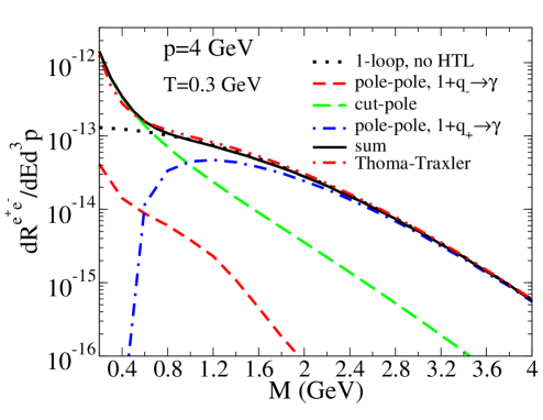
Figure 6: (Color online) Production rate of dileptons with momentum $p=4$ GeV, from thermally induced reactions, at a temperature $T=300$ MeV and for $\alpha_{s}=0.3$. Dotted line: Born term; short-dashed line: pole-pole contribution with particles having negative identical helicity over chirality ratio $\chi$; dot-dashed line: pole-pole contribution with particles having identical helicity over chirality ratio $\chi$; long-dashed line: cut-pole contribution; solid line: sum of all processes; and double dot-dashed line: Born term plus $\alpha^{2}\alpha_{s}$ contributions from Ref. thoma .

IV Dilepton Yield in Ultra-Relativistic Heavy-Ion Collisions

IV.1 Thermal Dileptons

High-$p_{T}$ real and virtual photons are preferentially emitted early during the QGP phase, when the temperature is largest. Explicit hydrodynamic calculations show that the space-time geometry of the fireball smoothly evolves from a 1-D to a 3-D expansion kolb . By the time the system reaches the temperature corresponding to the mixed phase in a first-order phase transition, the system is still dominated by a 1-D expansion kolb . For such a geometry, specific calculations flow suggest that the flow effect on photons and dileptons from the QGP is not large at RHIC and LHC for particles with transverse momentum $p_{T}>2$ GeV.

Assuming a 1-D expansion Bjorken that is cut off at a maximal space-time rapidity $\eta_{\rm max}$, the yield as a function of invariant mass $M$ and dilepton rapidity $y_{d}$ is given by the rate $R^{e^{+}e^{-}}=R^{e^{+}e^{-}}(\tau,\eta,\mathbf{r}_{\perp})$ as

$$\frac{dN^{e^{+}e^{-}}}{dM^{2}dy_{d}}=\int\tau d\tau d^{2}r_{\perp}d\eta\frac{dR^{e^{+}e^{-}}}{dM^{2}dy_{d}}\,.$$ (37)

Here $\tau$, $\eta$ and $\mathbf{r}_{\perp}$ are the proper time, space-time rapidity and the transverse coordinate respectively. In the remainder of this work the dependence of $R$ on $\tau$ and $\mathbf{r}_{\perp}$ will be omitted in the notation for brevity. As long as $y_{d}<<\eta_{\rm max}$ we can invoke boost invariance for $dR^{e^{+}e^{-}}/dy_{d}$ to argue that

$$\int\limits_{-\eta_{max}}^{\eta_{max}}d\eta\frac{dR^{e^{+}e^{-}}(\eta)}{dM^{2}dy}\Big{|}_{y=y_{d}}=\int\limits_{-\eta_{max}}^{\eta_{max}}d\eta\frac{dR^{e^{+}e^{-}}(y_{d})}{dM^{2}dy}\Big{|}_{y=\eta}=\frac{dR^{e^{+}e^{-}}(y_{d})}{dM^{2}}.$$ (38)

Hence the rate of lepton pairs with a fixed rapidity $y_{d}$ integrated over the entire longitudinal extent of the fireball is the same as the rate of all lepton pairs integrated over rapidity from the slice of the fireball at $\eta=y_{d}$. In the following we study only dileptons produced at mid-rapidity $y_{d}=0$. Their yield can now be written as

$$\frac{dN^{e^{+}e^{-}}}{dM^{2}dy_{d}}\Big{|}_{y_{d}=0}=\int\tau d\tau d^{2}r_{\perp}\frac{dR^{e^{+}e^{-}}(\eta=0)}{dM^{2}}=\int\tau d\tau d^{2}r_{\perp}\int dp_{T}p_{T}\int dp_{z}\frac{2\pi}{E_{0}}\frac{1}{2}\frac{dR^{e^{+}e^{-}}(\eta=0)}{d^{4}p}\,.$$ (39)

Here $E_{0}$ is the energy of the lepton pair in a local frame (where the temperature is defined) moving with rapidity $y=\frac{1}{2}\mbox{ln}\frac{E_{0}+p_{0}}{E_{0}-p_{0}}$ relatively to the fireball. In this local frame, the transverse and longitudinal momentum of the dilepton are $p_{T}$ and $p_{z}$ respectively. Then we have $p_{0}=\sqrt{p_{T}^{2}+p_{z}^{2}}$ and $E_{0}=\sqrt{M^{2}+p_{0}^{2}}$. The dilepton energy as seen from the fireball is $E=\sqrt{M^{2}+p_{T}^{2}}$.

At this point, we add two constraints in order to facilitate comparison with experimental data. First, we introduce a lower cutoff $p_{T{\rm cut}}$ for the transverse momentum of the lepton pair; second, a cut on the individual lepton rapidities which reflects the finite geometrical acceptance of any detector, is included, such that $\left|y_{e^{\pm}}\right|\leq y_{\rm cut}$. We introduce a multiplicative factor $P_{\rm cut}=P(|y_{e^{\pm}}|\leq y_{\mathrm{cut}},p_{T})$ to include the latter condition. In the center of mass frame of the lepton pair the distribution of positive leptons, normalized to unity, is given by

$$\frac{E^{+}_{cm}dP_{\gamma^{*}\to e^{+}e^{-}}}{d^{3}p^{+}_{cm}}=\frac{\delta(E^{+}_{cm}-\frac{M}{2})}{4\pi E^{+}_{cm}}.$$ (40)

Then the probability for a virtual photon with momentum $p_{T}$ at midrapidity to emit two leptons with rapidities $\left|y_{e^{\pm}}\right|\leq y_{\rm cut}$ can be obtained by a boost back to the lab frame as

$$P(|y_{e^{\pm}}|\leq y_{\mathrm{cut}},p_{T}) = \int\frac{d^{3}p^{+}_{cm}}{E^{+}_{cm}}\frac{E^{+}_{cm}dP_{\gamma\to e^{+}e^{-}}}{d^{3}p^{+}_{cm}}\Theta(|y_{e^{\pm}}|\leq y_{\rm cut})$$ (41)

$$= \int\frac{d\cos\theta d\phi}{\pi}\left(\frac{E^{+}}{M}\right)^{2}\Theta(|y_{e^{\pm}}|\leq y_{\rm cut}).$$

Note that in this frame

$$y_{e^{\pm}} = \frac{1}{2}\ln\frac{E^{\pm}+p^{\pm}_{z}}{E^{\pm}-p^{\pm}_{z}}\,,$$ (42)

$$E^{+} = \frac{M^{2}}{2(\sqrt{M^{2}+p_{T}^{2}}-p_{T}\cos\theta)}\,,$$ (43)

$$p_{z}^{\pm} = \pm E^{+}\sin\theta\,\sin\phi\,$$ (44)

and $E^{-}=E-E^{+}$.

The dilepton yield in a longitudinally expanding QGP is finally given by

$$\frac{dN^{e^{+}e^{-}}}{dM^{2}dy_{d}}=\int d\tau\,\tau\int_{0}^{R_{\perp}}dr\,r\int_{0}^{2\pi}d\phi\int_{p_{T_{\mathrm{cut}}}}^{\infty}dp_{T}\,p_{T}\int_{-\infty}^{\infty}dp_{z}\frac{2\pi}{E_{0}}\frac{1}{2}\frac{dR^{e^{+}e^{-}}}{d^{4}p}P(|y_{e^{\pm}}|\leq y_{\mathrm{cut}},p_{T})$$ (45)

The thermal-thermal yield at midrapidity is thus obtained by combining Eq. (18) and Eq. (45).

IV.2 Jet-Thermal Dileptons

In this subsection, we calculate the emission rate of dileptons from interaction of jets with the medium. The initial phase space distribution function for partons from jets produced in heavy ion collisions is simon2 ; lin

$$f_{q\bar{q}}^{\rm jet}(\vec{x},\vec{p},t_{0})=\frac{(2\pi)^{3}\mathcal{P}(\mathbf{r}_{\perp})}{g_{q}\tau p_{T}}\frac{dN_{q\bar{q}}^{\rm jet}}{dyd^{2}p_{T}}\delta(\eta-y)$$ (46)

in a boost invariant Bjorken scenario. $\eta$ is the space-time rapidity, $t_{0}$ the formation time of the jets and $\tau^{2}=t_{0}^{2}-z^{2}$. $dN_{q\bar{q}}^{\rm jet}/(dyd^{2}p_{T})$ is the spectrum of jets and $g_{q}$ is the spin-color degeneracy. $\mathcal{P}(\mathbf{r}_{\perp})$ represents the probability to create a jet at position $\mathbf{r}_{\perp}$ in the transverse plane. It is given by the product of the thickness functions of the colliding nuclei at $\mathbf{r}_{\perp}$ normalized to 1. For central collisions and assuming hard sphere nuclei, we have

$$\mathcal{P}(\mathbf{r}_{\perp})={2\over\pi R_{\perp}^{2}}\left(1-{r_{\perp}^{2}\over R_{\perp}^{2}}\right)\,\theta(R_{\perp}-r_{\perp})\,,$$ (47)

where $R_{\perp}=A^{1/3}1.2$ fm is the radius of the nucleus in the transverse plane. Since energy loss by bremsstrahlung involves only small $O(g_{\rm s}T/p)$ changes to the directions of particles, we suppose that jets keep propagating in straight lines after they are created. Then at any later time $t$

$$f_{q\bar{q}}^{\rm jet}(\vec{x},\vec{p},t)=f_{q\bar{q}}^{\rm jet}\left(\vec{x}-\hat{t}\frac{\vec{p}}{\left|\vec{p}\right|},\vec{p},t_{0}\right)$$ (48)

where $\hat{t}=t-t_{0}$ is the propagation time of the jet.

Energy loss can be described as a dependence of the parton spectrum $dN_{q\bar{q}}^{\rm jet}/dE$ on time. We will only be interested in the region around midrapidity later, so we can write

$$\frac{dN_{q\bar{q}}^{\rm jet}}{dyd^{2}p_{T}}\Big{|}_{y=0}=\Omega^{-1}\frac{dN_{q\bar{q}}^{\rm jet}}{EdE}$$ (49)

with a phase space factor $\Omega$. The evolution of the energy spectrum $dN_{q\bar{q}}^{\rm jet}(t)/dE$ is determined by the AMY evolution equations. Note that we do not need to specify the constant $\Omega$ to obtain the evolution of the spectrum. Here we quote only the basic formulas of the AMY formalism, which assumes that jets lose energy by inelastic processes only. More details can be found in AMY ; Jeon-Moore . This formalism has been applied in Ref. simon2 to successfully reproduce the $\pi^{0}$ spectra at RHIC. The parton spectrum $dN_{q\bar{q}}^{\rm jet}/dE$ depends on the energy lost, but not really on how this energy has been lost, such that using an another model for jet-quenching, like for example a model including elastic energy loss whdg05 , should not affect our following results for the dilepton production from jet-plasma interactions.

The evolution equations for the spectra are

$$\frac{d}{dt}\left(\frac{dN^{\rm jet}_{q\bar{q}}(p)}{dE}\right) = \int dk\!\left[\frac{dN^{\rm jet}_{q\bar{q}}(p{+}k)}{dE}\frac{d\Gamma^{q}_{\!qg}(p{+}k,k)}{dkdt}-\frac{dN^{\rm jet}_{q\bar{q}}(p)}{dE}\frac{d\Gamma^{q}_{\!qg}(p,k)}{dkdt}+2\frac{dN^{jet}_{g}(p{+}k)}{dE}\frac{d\Gamma^{g}_{\!q\bar{q}}(p{+}k,k)}{dkdt}\right]\,,$$

$$\frac{d}{dt}\left(\frac{dN^{\rm jet}_{g}(p)}{dE}\right) = \int dk\!\left[\frac{dN^{\rm jet}_{q\bar{q}}(p{+}k)}{dE}\frac{d\Gamma^{q}_{\!qg}(p{+}k,p)}{dkdt}{+}\frac{dN^{\rm jet}_{g}(p{+}k)}{dE}\frac{d\Gamma^{g}_{\!\!gg}(p{+}k,k)}{dkdt}\right.$$ (50)

$$\;\left.-\frac{dN^{\rm jet}_{g}(p)}{dE}\left(\frac{d\Gamma^{g}_{\!q\bar{q}}(p,k)}{dkdt}+\frac{d\Gamma^{g}_{\!\!gg}(p,k)}{dkdt}\Theta(2k{-}p)\!\!\right)\right],$$

with the transition rates

$$\frac{d\Gamma(p,k)}{dkdt}=\frac{C_{s}g_{\rm s}^{2}}{16\pi p^{7}}\frac{1}{1\pm e^{-k/T}}\frac{1}{1\pm e^{-(p-k)/T}}\times\left\{\begin{array}[]{cc}\frac{1+(1{-}x)^{2}}{x^{3}(1{-}x)^{2}}&(q\rightarrow qg)\\ N_{\rm f}\frac{x^{2}+(1{-}x)^{2}}{x^{2}(1{-}x)^{2}}&(g\rightarrow qq)\\ \frac{1+x^{4}+(1{-}x)^{4}}{x^{3}(1{-}x)^{3}}&(g\rightarrow gg)\\ \end{array}\right\}\times\int\frac{d^{2}{\bf h}}{(2\pi)^{2}}2{\bf h}\cdot{\rm Re}\>{\bf F}({\bf h},p,k)\,.$$ (51)

The integration over the range $k<0$ represents absorption of thermal gluons from the QGP; the range with $k>p$ represents annihilation with a parton from the QGP of energy $k{-}p$, while $0<k<p$ is the range of bremsstrahlung. In writing (50), we used $d\Gamma^{g}_{\!gg}(p,k)=d\Gamma^{g}_{\!gg}(p,p{-}k)$ and similarly for $g\rightarrow qq$. The $\Theta$-function in the loss term for $g\rightarrow gg$ prevents the double counting of final states. In Eq. (51) $C_{s}$ is the quadratic Casimir relevant for each process considered, and $x\equiv k/p$ is the momentum fraction of the gluon (or the quark, for the case $g\rightarrow q\bar{q}$). The factors $1/(1\pm e^{-k/T})$ are Bose enhancement or Pauli blocking factors for the final states. The vector ${\bf h}\equiv{\bf p}\times\mathbf{k}$ determines how non-collinear the final state is, and ${\bf F}({\bf h},p,k)$ is the solution of an integral equation describing how $\left|p-k;k\right>\left<p\right|$ evolves with time AMY .

The dileptons produced from the passage of jets through the QGP are finally obtained from Eq. (45) and from Eqs. (28) and (36) with the substitution $f^{q+\bar{q}}(E_{1})\rightarrow f_{q\bar{q}}^{\rm jet}(E_{1})$. Note that $\eta=0$ together with the boost invariance of the jet distribution imply that the longitudinal momentum of the jet parton vanishes. After some algebra, we get

$$\frac{dN_{\mathrm{jet-th}}}{dM^{2}dy_{d}} = \frac{4\alpha^{2}\sum_{f}\left(\frac{e_{f}}{e}\right)^{2}}{\pi M^{2}g_{q}}\int dt\int_{0}^{R_{\perp}}rdr\,\xi\int_{p_{T_{\mathrm{cut}}}}^{\infty}dp_{T}P(|y_{e^{\pm}}|\leq y_{\mathrm{cut}},p_{T})\int_{0}^{\infty}dq_{T}\int_{-\infty}^{\infty}dq_{z}\frac{1}{E_{0}}$$ (52)

$$\times\sum_{j=\pm}\Big{[}\frac{f_{\mathrm{FD}}(\omega_{j}(\left|\vec{q}\right|))}{2m_{F}^{2}}\frac{(\omega_{j}(\left|\vec{q}\right|)^{2}-\left|\vec{q}\right|^{2})}{\sqrt{1-\mbox{cos}^{2}\theta_{j}}}(1+j\frac{\left|\vec{q}\right|}{E_{1}^{j}}-j\frac{{\bf q}\cdot{\bf p}}{\left|\vec{q}\right|E^{j}_{1}})E^{j}_{1}\frac{dN_{q\bar{q}}^{\mathrm{jet}}(t)}{dy_{1}d^{2}p_{T_{1}}}\Big{|}_{y_{1}=0}$$

$$\quad+\int_{-\infty}^{\infty}d\omega f_{\mathrm{FD}}(\omega)\beta_{j}(\omega,\left|\vec{q}\right|)\left(1+j\frac{\left|\vec{q}\right|}{E_{1}}-j\frac{{\bf q}\cdot{\bf p}}{\left|\vec{q}\right|E_{1}}\right)\frac{E_{1}}{\sqrt{1-\mbox{cos}^{2}\theta}}\frac{dN_{q\bar{q}}^{\mathrm{jet}}(t)}{dy_{1}d^{2}p_{T_{1}}}\Big{|}_{y_{1}=0}\Big{]}$$

with $\left|\vec{q}\right|=\sqrt{q_{T}^{2}+q_{z}^{2}}$ and

$$\xi=\left\{\begin{array}[]{l}0\\ \displaystyle\frac{4}{R_{\perp}^{2}}\left(1-\frac{r^{2}+t^{2}}{R_{\perp}^{2}}\right)\\ \displaystyle\frac{4u_{0}}{\pi R_{\perp}^{2}}\left(1-\frac{r^{2}+t^{2}}{R_{\perp}^{2}}\right)+\frac{8tr}{\pi R_{\perp}^{4}}\sin u_{0}\,,\end{array}\right.$$ (56)

for the cases that $r^{2}+t^{2}-2tr>R_{\perp}^{2}$, $r^{2}+t^{2}+2tr\leq R_{\perp}^{2}$ and all other cases, respectively. Here we have defined

$$u_{0}=\arccos\frac{r^{2}+t^{2}-R_{\perp}^{2}}{2t\,r}\,.$$ (57)

The other quantities to be specified are

$${\bf q}\cdot{\bf p} = p_{T}\,q_{T}\,\mbox{cos}\,\theta_{\pm}+q_{z}^{2}\,,$$

$$\theta_{\pm} = \mbox{cos}^{-1}\left(\frac{p_{T}^{2}+q^{2}_{T}-(E_{0}-\omega_{\pm})^{2}}{2p_{T}q_{T}}\right)\,,$$ (58)

$$E_{1}^{\pm} = E_{0}-\omega_{\pm}\,.$$

We obtain the jet-thermal dilepton yield without HTL effects, i.e the Born term, by keeping only the pole-pole($q_{+}$) contribution in Eq. (52). In this case we have to substitute:

$$\beta_{\pm} \rightarrow 0\,,\qquad \frac{(\omega_{-}^{2}-\left|\vec{q}\right|^{2})}{2m_{F}^{2}} \rightarrow 0\,,$$ (59)

$$\frac{(\omega_{+}^{2}-\left|\vec{q}\right|^{2})}{2m_{F}^{2}} \rightarrow 1\,,\qquad (1+\frac{|\vec{q}|}{E_{1}^{+}}-\frac{{\bf q}\cdot{\bf p}}{|\vec{q}|E^{+}_{1}}) \rightarrow\frac{M^{2}}{2E_{1}E_{q}}\,,$$ (60)

$$\omega_{+} \rightarrow E_{q}=|\vec{q}|\,.$$ (61)

This leads to the final expression for the jet-thermal dilepton yield without HTL effects:

$$\frac{dN_{\mathrm{jet-th}}^{\mathrm{no-HTL}}}{dM^{2}dy_{d}} = \frac{2\alpha^{2}\sum_{f}\left(\frac{e_{f}}{e}\right)^{2}}{\pi g_{q}}\int dt\int_{0}^{R_{\perp}}rdr\,\xi\int_{p_{T_{\mathrm{cut}}}}^{\infty}dp_{T}\int_{0}^{\infty}dq_{T}\int_{-\infty}^{\infty}dq_{z}\frac{dN^{q\bar{q}}(t)}{dy_{1}d^{2}p_{T_{1}}}\Big{|}_{y_{1}=0}$$ (62)

$$\times\frac{1}{E_{0}E_{q}\sqrt{1-\mbox{cos}^{2}\theta_{+}}}\,f_{\mathrm{FD}}(E_{q})P(|y_{e^{\pm}}|\leq y_{\mathrm{cut}},p_{T})\,.$$

For a purely longitudinal expansion of the fireball Bjorken , at each point the temperature is evolving from some initial time $\tau_{i}$ as

$$T(\mathbf{r}_{\perp},\tau)=T(\mathbf{r}_{\perp},\tau_{i})\left(\frac{\tau_{i}}{\tau}\right)^{1/3}\,.$$ (63)

We assign the initial temperatures in the transverse direction according to the local density so that prlphoton ; prcdilep ; simon2

$$T(r_{\perp},\tau_{i})=T_{i}\left[2\left(1-\frac{r_{\perp}^{2}}{R_{\perp}^{2}}\right)\right]^{1/4}\,.$$ (64)

We assume a first-order phase transition and use

$$f_{\rm QGP}(\tau)=\frac{1}{r_{d}-1}\left(\frac{r_{d}\tau_{f}}{\tau}-1\right)$$ (65)

as the fraction of the QGP present during the mixed phase Bjorken . Here $r_{d}=g_{Q}/g_{H}$ is the ratio of the degrees of freedom in the two phases: $g_{Q}=42.25$ for a QGP with three flavors of quarks and $g_{H}=3$ for a simple gas of pions. $\tau_{f}$ is the time when the temperature reaches the critical temperature of 160 MeV (see Eqs. 63 and  64), marking the beginning of the mixed phase, and $\tau_{H}=r_{d}\tau_{f}$ is the time it ends, determined by the condition $f_{\rm QGP}=0$. However, since signals associated with jets are sensitive to early times, the order of the phase transition is not crucial. The $\tau$-integration in (45) is carried out from $\tau_{i}$ to $\tau_{H}$ and in addition it is scaled between $\tau_{f}$ and $\tau_{H}$ to account for the fact that only a fraction of the system is still a QGP, such that simon2

$$\int d\tau=\int\limits_{\tau_{i}}^{\tau_{f}}d\tau+\int\limits_{\tau_{f}}^{\tau_{H}}d\tau f_{\rm QGP}(\tau)\,.$$ (66)

V Drell-Yan and Heavy Flavour Decay

We calculate the Drell-Yan process to order $\mathcal{O}(\alpha_{s})$ in the strong coupling which is the leading order result with non-vanishing transverse momentum $p_{T}$ of the lepton pair. We also have to take into account virtual photon bremsstrahlung from jets. The total Drell-Yan yield is the sum of the direct and the Bremsstrahlung contributions, $\sigma_{\rm DY}=\sigma_{\rm direct}+\sigma_{\rm frag}$ qiu ; berger .

The direct contribution in collisions of two nuclei $A$ and $B$ is given by

$$\frac{d\sigma_{\rm direct}}{dM^{2}dy_{d}\,dp_{T}^{2}}=\frac{\alpha^{2}\alpha_{s}}{3M^{2}s_{NN}}\sum_{a,b}\int\frac{dx_{a}}{x_{a}x_{b}}f_{a/A}(x_{a},Q)f_{b/B}(x_{b},Q)\frac{\left|\bar{M}_{a+b\rightarrow c+\gamma^{*}}\right|^{2}}{s_{NN}x_{a}-\sqrt{s_{NN}}\sqrt{M^{2}+p_{T}^{2}}e^{y_{d}}}\,.$$ (67)

The squared scattering amplitudes $\left|\bar{M}_{a+b\rightarrow c+\gamma^{*}}\right|^{2}$ for the Compton and annihilation processes of two incoming partons can be found in guo . When $p_{T}$ and $M$ are both large and of the same order, the direct contribution is the dominant mechanism. However, when $\Lambda_{\rm QCD}\ll M\ll p_{T}$, logarithmic corrections with powers of $\ln(p_{T}^{2}/M^{2})$ are large. They can be effectively resummed into a virtual-photon fragmentation function $D_{\gamma^{*}/c}(z,Q_{F})$, giving rise to the fragmentation contribution

$$\frac{d\sigma_{\rm frag}}{dM^{2}dy_{d}\,dp_{T}^{2}} = \frac{\alpha}{3\pi M^{2}}\int\frac{dz}{z^{2}}\frac{d\sigma^{A+B\rightarrow c+d}}{dy_{d}\,dp_{cT}^{2}}\Big{|}_{p_{cT}=p_{T}/z}$$ (68)

$$\times D_{\gamma^{*}/c}(z,Q_{F})\,.$$

The cross sections for the production of a massless partons $c$ in $A+B$ collisions, $d\sigma^{A+B\rightarrow c+d}/dy_{d}\,dp_{cT}^{2}$, can be found in owens . The factorization scale $Q$ and the fragmentation scale $Q_{F}$ are both set to the order of the energy exchanged in the reaction $\sqrt{M^{2}+p_{T}^{2}}$ yellow_fai . The effect of varying the scale $Q=k\sqrt{p_{T}^{2}+M^{2}}$, from $k=1/2$ to $k=2$, introduces a variation of the dilepton yield by $\sim\pm$ 35 % relatively to $k=1$.

The typical fragmentation time of a jet into a virtual photon with large invariant mass $M$ scales like $1/M$. Thus dilepton with large mass $M$ can be created in the medium with rather small corrections due to energy loss of their parent jet, while low-$M$ dileptons should be formed outside the medium with their yield affected by the full energy loss suffered by the jet. Since the interesting region for the fragmentation process is for low masses $M$, where it is expected to be as important as the direct process, we assume that virtual photons fragment outside the medium after the parent jet has obtained its final energy. We define a medium-modified effective fragmentation function simon2

$$D_{\gamma^{*}/c}(z,Q_{F})=\int d^{2}r_{\perp}\mathcal{P}(\mathbf{r}_{\perp})\int dE_{f}\frac{z^{\prime}}{z}\frac{dN^{\rm jet}_{q\bar{q}}}{dE}(E_{f};E_{i})D^{0}_{\gamma^{*}/q}(z^{\prime},Q_{F})$$ (69)

where $z=p_{T}/E_{i}$ and $z^{\prime}=p_{T}/E_{f}$. $dN^{\rm jet}_{q\bar{q}}/dE$ is the probability to for a given quark with final energy $E_{f}$ when the initial jet is a particle of type $c$ and energy $E_{i}$, given by the solutions to Eq. (50), $D^{0}_{\gamma^{*}/q}$ is the leading order vacuum fragmentation function from berger ; qiu . The factor $\mathcal{P}(\mathbf{r}_{\perp})$ is introduced to take care of the spatial distribution of jets and their propagation length in the medium.

We implement our cuts for the Drell-Yan process as well, so that the final yield is given by

$$\frac{dN_{\rm DY}}{dM^{2}dy_{d}} = \frac{2\langle N_{\rm coll}\rangle}{\sigma_{in}}\int\limits_{p_{T{\rm cut}}}^{\infty}dp_{T}\,p_{T}\Big{[}K_{dir}\frac{d\sigma_{\rm direct}}{dM^{2}dy_{d}\,dp_{T}^{2}}+K_{frag}\frac{d\sigma_{\rm frag}}{dM^{2}dy_{d}\,dp_{T}^{2}}\Big{]}P(|y_{e^{\pm}}|\leq y_{cut},p_{T})\,.$$ (70)

where $K_{dir}$ and $K_{frag}$ are introduced to take care of higher order effects. We reproduce the Drell-Yan isolated muons from $\sqrt{s_{NN}}$=630 GeV $p+\bar{p}$ data at CERN UA1 , for low invariant masses ($M<2.5$ GeV) and high transverse momentum ($p_{T}>6$ GeV), with a constant factor $K_{dir}=1.5$. We also take $K_{frag}=1.5$, quite in line with the $K$-factor used for real photons from jet-fragmentation in Ref. simon2 . While we assume the $K$-factors to be constant, they should be in principle $\sqrt{s_{NN}}$, $p_{T}$ and $M$ dependent. However, an estimate of the variation of $K_{dir}$ with those parameters can be found in Ref. berger . For example, next-leading order effects for the direct Drell-Yan contribution at $\sqrt{s_{NN}}=2$ TeV in the range $10<p_{T}<20$ GeV would vary within 10$\%$ from $M\sim 2.5$ GeV to $M\sim 4.5$ GeV.

Here we assume $\langle N_{\rm coll}\rangle=975$, $\sigma_{in}=40$ mb for RHIC jeon and $\langle N_{\rm coll}\rangle=1670$, $\sigma_{in}=72$ mb for the LHC yellow . In our calculations we use CTEQ5 parton distribution functions cteq5 with EKS98 shadowing corrections eskola .

The main background at RHIC energies for the dilepton production processes considered so far is expected to be decay of open charm and bottom mesons ralf . During the initial hard scattering, $c\,\bar{c}$ ($b\bar{b}$) pairs are produced and can thereafter fragment into $D(B)$ and $\bar{D}(\bar{B})$ mesons. We consider here only correlated decay, which happens when a positron coming from the semileptonic decay of a $D(B)$ is measured together with the electron from the semileptonic decay of a $\bar{D}(\bar{B})$. The results for heavy quark decay have been obtained with the techniques of Ref. mangano . Collisional energy loss of the heavy quarks propagating in the QGP heavy_q has not been included. Since this constitutes a background to our process, we adopt this conservative point of view.

VI Results

We choose the same parameterization of the plasma phase that was previously used successfully in the studies of high simon2 and low to intermediate $p_{T}$ photons simon . For central Au+Au collisions at RHIC we have an initial temperature $T_{i}$=370 MeV and initial time $\tau_{i}$=0.26 fm/c for the plasma phase, corresponding to the particle rapidity density $dN/dy$=1260 prcdilep . This latest value is obtained from the measured pseudo-rapidity distribution of charged particles $dN_{ch}/d\eta$ phobos : $dN/dy\sim\frac{3}{2}|d\eta/dy|dN_{ch}/d\eta$, where $|d\eta/dy|\sim$ 1.2 around $y=0$. For LHC, our initial conditions are $T_{i}$=845 MeV and $\tau_{i}$=0.088 fm/c corresponding to $dN/dy$=5625 prcdilep ; kms . For the processes involving the QGP, we assume three light flavors and we fix $\alpha_{s}=0.3$. As the jets are defined to be particles having a transverse momentum greater than a scale $p_{Q}$, with $p_{Q}\gg 1$GeV, we have set the dilepton momentum cutoff $p_{T_{\mathrm{cut}}}$ high enough to avoid any sensitivity to the choice of $p_{Q}$. We take $p_{T_{\mathrm{cut}}}=$ 4(8) GeV for RHIC (LHC). The cuts on leptons rapidities emulate the PHENIX experiment at RHIC, $y_{\mathrm{cut}}$=0.35, while we use $y_{cut}=$0.5 at LHC.

The dileptons produced at RHIC by the interaction of jets with the medium are shown in Fig. 7. Dileptons from jet-pole interactions, i.e. from annihilation of a jet parton with a $(q_{-})$-mode, are negligible, while the jet-pole interactions involving $(q_{+})$-modes tends toward the Born term at high invariant mass, as it was the case for thermal-thermal reactions in Fig. 6. On the other hand dileptons from jet-cut interactions do not behave like the cut-pole process in Fig. 6. They become the dominant contribution at high-$M$. The expressions for the cut-pole process, shown in Fig. 4b+c, involve the functions $\beta_{\pm}(\left|\vec{q}\right|)$ with $\beta_{\pm}(\left|\vec{q}\right|)\rightarrow 0$ for $\left|\vec{q}\right|\gg T$. When $M$ is large, in order to keep the value of $\left|\vec{q}\right|$ modest, the energy $E_{1}$ of the incoming parton has to be large: $E_{1}\geq M^{2}/4\left|\vec{q}\right|$. As the thermal phase space distribution function $f_{FD}$ decreases exponentially for large $E_{1}$, the cut-pole contribution turns out to be negligible for large $M$. However, when the incoming particle is a jet with a power-law distribution, high values of $E_{1}$ are not suppressed and the cut-pole contribution is important. Therefore the sum of all the jet-thermal processes with HTL effects included (solid line), is more important than the jet-thermal contribution without HTL effects (double dot-dashed line) by more than a factor 2 for $M$ above 8 GeV. For $M$ below 1 GeV HTL corrections increase the Born term by one order of magnitude, because of the $1/M^{2}$ behavior in Eq. (52). We have verified that when extrapolated to $M=0$, the cut-pole contribution reproduces the result for the jet-photon conversion in the QGP simon2 , such that $E^{\gamma^{*}}dR_{\mbox{cut-pole}}(p,M\to 0)/d^{3}p=E^{\gamma}dR_{\mbox{jet-th}}(p)/d^{3}p$.

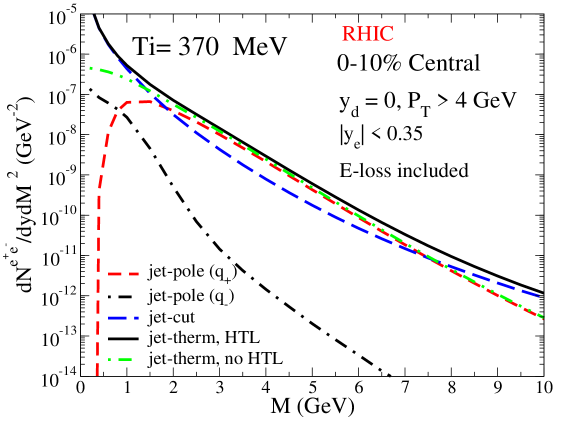
Figure 7: (Color online) High-momentum dileptons produced from the interaction of jets with QGP in Au+Au collisions at 200 GeV (RHIC). The initial temperature is $T_{i}$=370 MeV. Short-dashed line: interaction of jets with poles with positive $\chi$; dot-dashed line: interaction of jets with poles with negative $\chi$; long-dashed line: interaction of jets with cuts; solid line: sum of the latter processes; and double dot-dashed line: interaction of jet with QGP without HTL effects (Born term). See text for details.

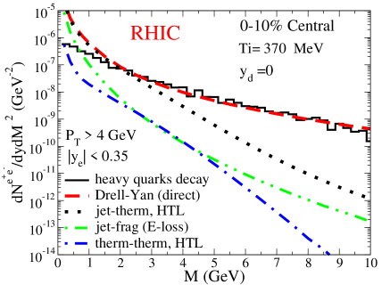
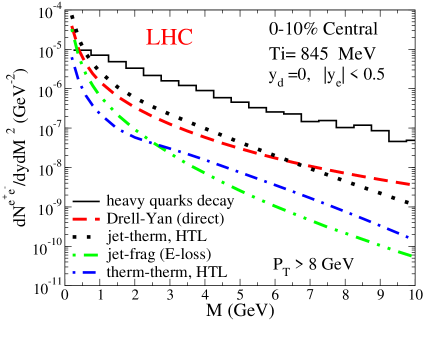
Figure 8: (Color online) Sources of high-$p_{T}$ dileptons in central Au+Au collisions at RHIC (left) and Pb+Pb at the LHC (right). Solid lines: semileptonic decay of heavy quarks; dashed lines: direct Drell-Yan contribution; dotted lines: jet-thermal interaction with HTL effects; double dot-dashed lines: jet-fragmentation process; and dot-dashed lines: thermal dilepton production with HTL effects.

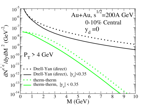
Figure 9: (Color online) Effect of the cut on leptons rapidities for direct Drell-Yan (top) and thermal dileptons (bottom) without HTL effects at RHIC. The dotted lines include all leptons from the respective process while the solid lines include only leptons having absolute value of rapidity smaller than 0.35.

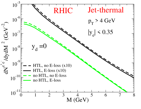
Figure 10: (Color online) Effect of jet energy loss in jet-thermal production of dileptons at RHIC, with HTL effects (top) and without (bottom). The solid lines include the effect of energy loss, while the dashed lines don’t. The results for jet-plasma interactions with HTL have been rescaled by a factor 10 for clarity.

In Fig. 8 we show the mass spectrum of dileptons in central Au+Au collisions at RHIC ($\sqrt{s_{NN}}=200$ GeV) and central Pb+Pb collisions at LHC ($\sqrt{s_{NN}}=5.5$ TeV). For both collider energies, the jet-thermal contribution exceeds the thermal dilepton production by an order of magnitude, which was also the case for high-$p_{T}$ photon production simon2 ; prlphoton . However, at RHIC the dominant sources of dileptons for $M>3$ GeV are heavy quark decay and the direct Drell-Yan process. At intermediate mass, between 1 GeV and 3 GeV, the jet-thermal contribution is as important as these two processes. Below 1 GeV, the fragmentation of jets into virtual photons turns out to be comparable to the direct Drell-Yan production and the jet-thermal contribution. At LHC, the whole range of invariant mass is dominated by charm decay, but on the other hand the jet-thermal lepton pairs exceed the direct Drell-Yan yield below 7 GeV. We want to stress that energy loss of heavy partons has not been included here, so that the heavy quark contribution is likely an upper limit of what is to be expected. Lepton pair production from jet-plasma interactions being as important as this upper limit background at RHIC for $1<M<3$ GeV, we thus expect the experimental detection of a jet-plasma contribution to be feasible. For real photons, the inclusive yield is largely dominated by the background coming from the decay of neutral mesons phe_pho , in the region where the jet-thermal contribution is expected to be maximal.

While the thermally induced dilepton yield may be strongly affected by initial conditions like temperature and thermalization time, this is not the case for the jet-plasma contribution. This is due to the phase-space distribution of jets, which has a weak dependence on temperature and makes the dilepton production less pronounced in the early time of the QGP evolution (see Ref. simon2 for a more detailed discussion of the effect of initial conditions on real photon production). The same argument can be also used to estimate the effects of a possible chemical non-equilibrium on the jet-plasma contribution. On one hand, lower quark fugacities suppress the dilepton emission at a given temperature, but on the other hand, smaller fugacities would imply larger temperature, thus increasing the dilepton yield. The interplay of those effects was studied in Ref. rapp_2001 for thermally induced dileptons, showing a suppression in the yield for large invariant masses at RHIC (a factor $\sim$ 2 of suppression for $M\sim$ 4 GeV). However, for jet-medium interactions the fugacities would enter into the production rate only linearly rather than quadratically for thermally induced dileptons, thus the effect of chemical non-equilibrium should be less pronounced.

The effect of the momentum cut on single lepton rapidity is shown in Fig. 9 at RHIC energy for Drell-Yan and thermal-thermal processes without HTL corrections. For both cases, the cut reduces the yield by a factor $\sim$ 3 and is almost independent of $M$, except in the low mass region. When $M$ is small, the lepton rapidities tend to be very close to the pair rapidity $y_{d}=0$, making the cut less important.

The effect of energy loss on the jet-thermal lepton pair production is explored in Fig. 10 for RHIC. We observe that for the case without HTL effects (Born term), dileptons are reduced by about $30\%$ for $M\sim$ 1 GeV, while the suppression decreases with increasing invariant mass, reaching about 15% above $M$ = 4 GeV. For a given invariant mass $M$ and jet energy $E_{1}$, the minimum energy for the thermal parton is $E_{2_{min}}=M^{2}/4E_{1}$. This minimal value is then favored by the steep thermal spectrum, leading to a dependence of the yield that is roughly given by $\exp(-M^{2}/4E_{1}T)$. This implies that dileptons with large mass $M$ are more likely to be emitted at times where the temperatures $T$ is still high which favors small jet propagation time and small energy loss. Including HTL effects leads to a suppression of about $30\%$ for the range dominated by the cut-pole contribution, $M<$ 2 GeV and $M>7$ GeV. The region $2<M<7$ GeV, dominated by the pole-pole contribution, shows a weaker suppression, equivalent in magnitude to that of the Born term in the corresponding invariant mass range. The suppression factor is weaker for dileptons from jet-medium interactions than for high-$p_{T}$ pions, where a large suppression factor ($\sim 4-5$) has been observed at RHIC phenix2 . This can be understood because dileptons can be produced at any point during the propagation of the jet in the medium, whereas pions, due to their large formation time, are produced after a jet has left the medium, and thus they suffer from the full loss of energy

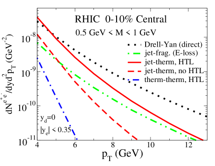
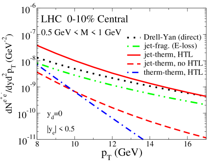
Figure 11: (Color online) $p_{T}$ distribution of dileptons, integrated in the range $0.5<M<1$ GeV, for RHIC (left) and the LHC (right). Dotted lines: direct Drell-Yan process; double dot-dashed lines: jet-fragmentation process; solid lines: jet-thermal process with HTL effects; dashed lines: jet-thermal process without HTL effects; and dot-dashed lines: thermal induced reactions with HTL effects.

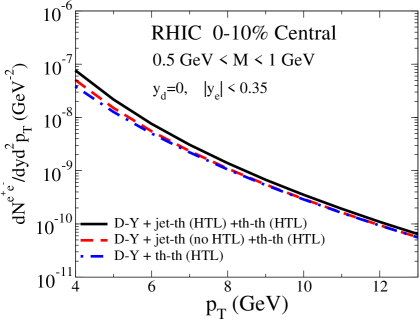
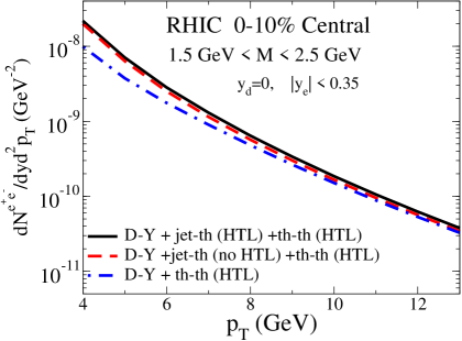
Figure 12: (Color online) $p_{T}$ distribution of dileptons, integrated in the range $0.5<M<1$ GeV (left panel) and $1.5<M<2.5$ GeV (right panel), for central Au+Au at RHIC. Solid line: sum of Drell-Yan process, jet-thermal and thermal-thermal process with HTL effects; dashed line: sum of Drell-Yan process, jet-thermal without HTL and thermal-thermal with HTL effects; and dot-dashed line: sum of Drell-Yan process and thermal-thermal reactions with HTL effects.

It is also interesting to discuss the dilepton yield as a function of the dilepton transverse momentum $p_{T}$ in certain windows of the mass $M$. This is done by substituting the integral over $p_{T}$ in Eqs. (45) and (70), by $\int dM^{2}/(2\pi p_{T})$. The results for RHIC and the LHC are displayed in Fig. 11, for the mass integrated in the range $0.5<M<$1 GeV. The ordering of the contributing sources here is very similar to the one seen for real photons as a function of $p_{T}$ in Ref. simon2 . The direct component of the Drell-Yan process dominates for high-$p_{T}$ dileptons at RHIC while the jet-thermal contribution, with HTL, dominates for $p_{T}<$5 GeV. The hard thermal loop calculation enhances this yield by more than a factor 4 compared to the jet-thermal contribution without HTL. At the LHC, jet-thermal dileptons (HTL effects included) are the most important source in the entire $p_{T}$ range, $8<p_{T}<17$ GeV. The jet-thermal interaction appears to be as important for dileptons as it was for real photon production.

The total direct dilepton spectrum for RHIC is shown in the left panel of Fig. 12. The solid line includes Drell-Yan and QGP contribution (jet-thermal and thermal-thermal) with HTL effects. Leaving out the HTL resummation for jet-thermal dileptons (dashed line) reduces the yield by a factor $\sim 1.5$ around $p_{T}$=4 GeV. The absence of any jet-thermal interactions at all (dot-dashed line) would reduce the total yield by a factor $\sim 2$ at $p_{T}$=4 GeV. This emphasizes the importance of this process in the presence of a QGP.

The only potentially important contribution that is not included in our work is in-medium bremsstrahlung ($q\,i\rightarrow q\,i\gamma^{*}$) and annihilation ($q\bar{q}i\rightarrow\gamma^{*}i$) of an incoming thermal parton or jet, where $i$ denotes a quark, antiquark or gluon. This goes beyond the current formulation of AMY. However, they have been calculated in Ref. Aurenche:2002wq for the case of incoming thermal partons, showing that for low mass dileptons, the bremsstrahlung and annihilation more than double the contribution obtained from $2\rightarrow 2$ processes ($q+g\rightarrow q+\gamma^{*},q+\bar{q}\rightarrow g+\gamma^{*}$). It thus turns out that thermally induced bremsstrahlung and annihilation are as important relatively to $2\rightarrow 2$ processes, no matter if the photons are virtual or real Arnold:2001ms . On the other hand, for the case of real photons and incoming jets, it has been shown in Ref. simon2 that those bremsstrahlung and annihilation processes are reduced by a factor 3-4, relatively to the in-medium jet-photon conversion process. This is because the momentum distribution of jets is less steep than the thermal one, making the jet-photon conversion the most important in-medium process. Therefore, if one assumes that the in-medium jet-bremsstrahlung contributes in the same way to virtual and to real photons, it would enhance the solid line by less than 15$\%$.

Finally, the right panel of Fig. 12 shows the dilepton spectrum for an another invariant mass window. It is located at higher values $1.5<M<2.5$ GeV between the $\phi$ and the $J/\psi$ masses. As we could have expected from Fig. 7, the effect of the HTL resummation is not very important for this mass window. However interactions of jets with the plasma are still a very important source of dileptons, and this should be detectable.

VII Summary and Conclusions

In this work we presented calculations of different sources of lepton pairs in high energy nuclear collisions. We take into account Drell-Yan, fragmentation from jets, QGP contributions and heavy quark decay. Hard thermal loop resummation has been included in the calculation of the leading order photon self-energy. We explicitly checked that the imaginary part of this self-energy, evaluated within finite-temperature field theory, and a different approach starting from relativistic kinetic theory and using the corresponding Feynman amplitudes, lead to the same results. We obtain the jet-plasma interaction by substituting the phase-space distribution of one incoming thermal parton, by the distribution of jets. While the HTL corrections are important for thermal-thermal processes at low-invariant mass, they are important for both low and high invariant mass when the incoming parton is a jet.

For the high momentum window investigated here, $p_{T}>4$ GeV, dilepton emissions due to jet-plasma interactions are found to be much larger than thermal dilepton emission. At low to intermediate dilepton mass, productions from jet-plasma interactions are comparable in size to the Drell-Yan contribution and constitute a good signature for the presence of a quark gluon plasma provided the dominant background of heavy quark decay could be subtracted. The AMY formalism has been used to account for energy loss of jets in the QCD plasma; this energy degradation reduces the effect of jet-thermal processes by $\sim$ 30%. Further study involving heavy quark energy loss will be needed to obtain a better estimate of this channel, together with an explicit calculation of dileptons from medium-induced bremsstrahlung.

- (1) E.L. Feinberg, Nuovo Cim. A 34, 391 (1976).
- (2) E. V. Shuryak, Phys. Lett. B 78, 150 (1978) [Sov. J. Nucl. Phys. 28, 408.1978 YAFIA,28,796 (1978 YAFIA,28,796-808.1978)].
- (3) R. J. Fries, B. Müller and D. K. Srivastava, Phys. Rev. Lett 90, 132301 (2003).
- (4) S. Turbide, C. Gale, S. Jeon and G. D. Moore, Phys. Rev. C 72, 014906 (2005).
- (5) S. D. Drell and T. M. Yan, Phys. Rev. Lett. 25, 316 (1970).
- (6) K. Kajantie, J. I. Kapusta, L. McLerran and A. Mekjian, Phys. Rev. D 34, 2746 (1986).
- (7) J. Kapusta, L. D. McLerran and D. K. Srivastava, Phys. Lett. B 283, 145 (1992).
- (8) T. Altherr and P.V. Ruuskanen, Nucl. Phys. B 380, 377 (1992).
- (9) C. Gale and P. Lichard, Phys. Rev. D 49, 3338 (1994).
- (10) R. Rapp and J. Wambach, Eur. Phys. J. A 6, 415 (1999).
- (11) D. K. Srivastava, C. Gale and R. J. Fries, Phys. Rev. C 67, 034903 (2003).
- (12) A. Shor, Phys. Lett. B 233, 231 (1989) [Erratum-ibid. B 252, 722 (1990)].
- (13) K. Geiger and J. I. Kapusta, Phys. Rev. Lett. 70, 1920 (1993).
- (14) S. S. Adler et al. (PHENIX Collaboration), Phys. Rev. Lett. 91, 072301 (2003).
- (15) J. Adams et al. (STAR Collaboration), Phys. Rev. Lett. 91, 172302 (2003).
- (16) C. Adler et al. (STAR Collaboration), Phys. Rev. Lett. 90, 082302 (2003).
- (17) A numerical error as been found in the program used to perform the calculations in Ref. prcdilep . The present paper thus constitutes an erratum and an update.
- (18) M. Gyulassy and M. Plümer, Phys. Lett. B 243, 432 (1990).
- (19) X. N. Wang, M. Gyulassy and M. Plümer, Phys. Rev. D 51, 3436 (1995).
- (20) P. Arnold, G. D. Moore and L. Yaffe, JHEP 0111, 057 (2001); JHEP 0206, 030 (2002).
- (21) A. B. Migdal, Phys. Rev. 103, 1811 (1956).
- (22) E. Braaten and R.D. Pisarski, Nucl. Phys. B 337, 569 (1990).
- (23) E. Braaten, R.D. Pisarski and T.C. Yuan, Phys. Rev. Lett. 64, 2242 (1990).
- (24) S. M. H. Wong, Z. Phys. C 53, 465 (1992).
- (25) M.H. Thoma and C.T. Traxler, Phys. Rev. D 56, 198 (1997).
- (26) C. Gale and J. Kapusta, Nucl. Phys. B 357, 65 (1991).
- (27) M. Le Bellac, Thermal Field Theory,(Cambridge University Press, 1996).
- (28) J. Kapusta, Finite-Temperature Field Theory, (Cambridge University Press, 1989).
- (29) J. Kapusta, P. Lichard and D. Seibert, Phys. Rev. D44, 2774 (1991) [erratum-ibid. D47, 4171 (1991)].
- (30) M.E. Peskin and D.V. Schroeder, An Introduction to Quantum Field Theory, (Perseus Books, 1995).
- (31) H.A. Weldon, Phys. Rev. D 28, 2007 (1983).
- (32) P.F. Kolb and U. Heinz, nucl-th/0305084.
- (33) D.K. Srivastava, M.G. Mustafa and B. Müller, Phys. Rev. C 56, 1064 (1997).
- (34) J.D. Bjorken, Phys. Rev. D 27, 140 (1983).
- (35) Z. Lin and M. Gyulassy, Phys. Rev. C 51, 2177 (1995).
- (36) S. Jeon and G.D. Moore, Phys. Rev. C 71, 034901 (2005).
- (37) S. Wicks, W. Horowitz, M. Djordjevic and M. Gyulassy, nucl-th/0512076.
- (38) J. Qiu and X. Zhang, Phys. Rev. D 64, 074007 (2001).
- (39) E. L. Berger, J. Qiu, and X. Zhang, Phys. Rev. D 65, 034006 (2002).
- (40) X. Guo, Phys. Rev. D 58, 036001 (1998).
- (41) K.J. Eskola, V.J. Kolhinen and C.A. Salgado, Eur. Phys. J. C 9, 61 (1999).
- (42) H.L. Lai et al., Eur. Phys. J. C 12, 375 (2000).
- (43) J.F. Owens, Rev. Mod. Phys. 59, 465 (1987).
- (44) G. Fai, J.W. Qiu and X.F. Zhang, Hard Probes in Heavy-Ion Collisions at the LHC, Ed. M. Mangano, H. Satz and U. Wiedemann, (2004), p. 65.
- (45) UA1 Collab., C. Albajar et al., Phys. Lett. B 209, 397 (1988).
- (46) S. Jeon, J.J. Marian and I. Sarcevic, Phys. Lett. B 562, 45 (2003).
- (47) F. Arleo et al., hep-ph/0311131
- (48) R. Rapp, preprint nucl-th/0409054.
- (49) M. L. Mangano, P. Nason, and G. Ridolfi, Nucl. Phys. B 373, 295 (1992).
- (50) G. D. Moore and D. Teaney, preprint hep-ph/0412346.
- (51) S. Turbide, R. Rapp, and C. Gale, Phys. Rev. C 69, 014903 (2004).
- (52) PHOBOS Collaboration (B.B. Back et al.), Phys. Rev. C65, 061901 (2002).
- (53) S.S. Adler et al., Phys. Rev. Lett. 94, 232301 (2005).
- (54) R. Rapp, Phys. Rev. C 69, 054907 (2001).
- (55) P. Aurenche, F. Gelis, G. D. Moore and H. Zaraket, JHEP 0212, 006 (2002).
- (56) P. Arnold, G. D. Moore and L. G. Yaffe, JHEP 0112, 009 (2001).