Estimate of the Hadronic Production of the Doubly Charmed Baryon $\Xi_{cc}$ under GM-VFN Scheme

Abstract

Hadronic production of the doubly charmed baryon $\Xi_{cc}$ ($\Xi^{++}_{cc}$ and $\Xi^{+}_{cc}$) is investigated under the general-mass variable-flavor-number (GM-VFN) scheme. The gluon-gluon fusion mechanism and the intrinsic charm mechanisms, i.e. via the sub-processes $g+g\to(cc)[^{3}S_{1}]_{\bar{3}}+\bar{c}+\bar{c}$, $g+g\to(cc)[^{1}S_{0}]_{6}+\bar{c}+\bar{c}$; $g+c\to(cc)[^{3}S_{1}]_{\bar{3}}+\bar{c}$, $g+c\to(cc)[^{1}S_{0}]_{6}+\bar{c}$ and $c+c\to(cc)[^{3}S_{1}]_{\bar{3}}+g$, $c+c\to(cc)[^{1}S_{0}]_{6}+g$, are taken into account in the investigation, where $(cc)[^{3}S_{1}]_{\bar{3}}$ (in color $\bar{3}$) and $(cc)[^{1}S_{0}]_{6}$ (in color $6$) are two possible $S$-wave configurations of the doubly charmed diquark pair $(cc)$ inside the baryon $\Xi_{cc}$. Numerical results for the production at hadornic colliders LHC and TEVATRON show that both the contributions from the doubly charmed diquark pairs $(cc)[^{1}S_{0}]_{6}$ and $(cc)[^{3}S_{1}]_{\bar{3}}$ are sizable with the assumption that the two NRQCD matrix elements are equal, and the total contributions from the ‘intrinsic’ charm mechanisms are bigger than those of the gluon-gluon fusion mechanism. For the production in the region of small transverse-momentum $p_{t}$, the intrinsic mechanisms are dominant over the gluon-gluon fusion mechanism and they can raise the theoretical prediction of the $\Xi_{cc}$ by almost one order.

PACS numbers: 14.20.Lq, 13.85.Ni, 12.38.Bx

I Introduction

The heavy hadron $\Xi^{+}_{cc}$ may have been observed by SELEX Collaboration alreadyexp ; exp2 , although some commentscomm pointed out that the measured lifetime is much shorter and the production rate is much larger than most of the theoretical predictions the ; baranov ; kiselev1 ; kiselev2 ; kiselev3 . It is predicted that at the fixed target experiment, only about $10^{-5}$ of $\Lambda_{c}^{+}$ events in its total sample are producted by $\Xi^{+}_{cc}$, however the SELEX collaboration has found that almost $20\%$ of $\Lambda_{c}^{+}$ events in its total sample are producted by $\Xi^{+}_{cc}$.

In the literature, most of the perturbative QCD (pQCD) calculations and predictions for $\Xi_{cc}$ hadroproduction are based on the ‘gluon-gluon fusion mechanism’ i.e. that via the subprocess, $g+g\to(cc)[^{3}S_{1}]_{\bar{3}}+\bar{c}+\bar{c}$ only. Whereas, the subprocess $g+g\to(cc)[^{1}S_{0}]_{6}+\bar{c}+\bar{c}$ may also contribute to the productionmajp . It is because that $\Xi^{+}_{cc}$ and $\Xi^{++}_{cc}$ contain the higher components $(ccqg)$ (here $q=u,d$) etc in their Fock space expansion, so the corresponding subprocess should be taken into account.

The discussion shown in Ref.majp indicates that an inclusive production rate of $\Xi^{+}_{cc}$ or $\Xi^{++}_{cc}$ can be factorized into two parts, one part is to produce two free $c$ quarks, which can be calculated by pQCD, another part is to make these two free $c$ quarks into a $cc$ diquark pair: $(cc)_{\bf\bar{3}}[^{3}S_{1}]$ or $(cc)_{\bf 6}[^{1}S_{0}]$, then the diquark pair hadronizing either into $\Xi^{+}_{cc}$ by absorbing a quark $d$ or into $\Xi^{++}_{cc}$ by absorbing a quark $u$ for $(cc)_{\bf\bar{3}}[^{3}S_{1}]$, or either into $\Xi^{+}_{cc}$ by absorbing a quark $d$ or into $\Xi^{++}_{cc}$ by absorbing a quark $u$ but both absorbing an extra soft gluon for $(cc)_{\bf 6}[^{1}S_{0}]$, all of which can be attributed to non-relativistic QCD (NRQCD) matrix elements nrqcd . In most of the existent calculations for the hadronic production of $\Xi_{cc}$, the $cc$ diquark pair is assumed to be in ${}^{3}S_{1}$ configuration and in the color representation ${\bf\bar{3}}$ ($(cc)_{\bf\bar{3}}[^{3}S_{1}]$). Whereas according to power counting in velocity $v_{c}$, the velocity of the heavy $c$ quarks in the baryon, the NRQCD matrix elements $h_{1}$ and $h_{3}$ (defined in Eq.(3)) for the nonperturbative transition, which correspond to the two configurations of the diquark pair ($h_{1}$ is that for $(cc)_{\bf\bar{3}}[^{3}S_{1}]$ and $h_{3}$ is that for $(cc)_{\bf 6}[^{1}S_{0}]$), are at the same order of $v_{c}$ majp . Hence to give a full estimation of the hadronic production of $\Xi_{cc}$, we think that $(cc)_{\bf\bar{3}}[^{3}S_{1}]$ and $(cc)_{\bf 6}[^{1}S_{0}]$ should be treated on the equal footing.

Moreover, as pointed out in Refs.qiao ; zqww , the so-called ‘intrinsic’ charm mechanism can give sizable contribution to the charmonium hadroproductionqiao , and to the $B_{c}$ hadroproduction, especially in small $p_{t}$ regionzqww . Therefore, in addition to considering two configurations of diquark pair in different color representation ${\bf\bar{3}}$ and ${\bf 6}$ for the gluon-gluon fusion mechanism, it is also interesting to see how important of the ‘intrinsic’ charm mechanisms via the sub-processes $g+c\to(cc)[^{3}S_{1}]_{\bf\bar{3}}+\bar{c}$, $g+c\to(cc)[^{1}S_{0}]_{\bf 6}+\bar{c}$ and $c+c\to(cc)[^{3}S_{1}]_{\bf\bar{3}}+g$, $c+c\to(cc)[^{1}S_{0}]_{\bf 6}+g$, in hadronic production of $\Xi^{+}_{cc}$ and $\Xi^{++}_{cc}$ precisely.

Principally, the ‘intrinsic’ charm mechanism induced by the heavy charm quark is greatly suppressed by the parton distributions in comparison with the valance and the sea of light quarks and gluon, but it is ‘compensated’ by ‘greater phase space’ and lower order of interaction coupling of QCD. Namely the ‘intrinsic’ processes are $2\to 2$ sub-processes at the order of ${\cal O}(\alpha_{s}^{3})$, while for the gluon-gluon fusion subprocess, its leading contribution starts at ${\cal O}(\alpha_{s}^{4})$ and is a $2\to 3$ process.

For a fixed target experiment which can reach to the region of very small transverse momentum $p_{t}$, the production of the doubly charmed baryon $\Xi_{cc}$ should additionally involve more ‘mechanisms’, such as the mechanisms of the so-called intrinsic charm fusion with the subprocesses $c+c\to(cc)[^{3}S_{1}]_{\bf\bar{3}}$ and $c+c\to(cc)[^{1}S_{0}]_{\bf 6}$, which contribute to the production only with very small $p_{t}$ but whose nature essentially is non-perturbative for QCD. The theoretical predictions on the hadronic production rate all can be based upon the perturbative QCD (pQCD) only, though the existent ones are orders of magnitude smaller than the SELEX observation as pointed out by Ref.comm . Nevertheless, we think that it is worthwhile to consider more mechanisms than that in the existent predictions, and to use the updated parton distribution functions (PDFs) in the general-mass variable-flavor-number (GM-VFN) scheme to re-estimate the $\Xi_{cc}$ hadroproduction so as to cover a so widen $p_{t}$ region as pQCD is applicable. Especially, more attention to the so-called intrinsic charm production mechanism, that is through the subprocesses $g+c\to(cc)[^{3}S_{1}]_{\bf\bar{3}}+\bar{c}$, $g+c\to(cc)[^{1}S_{0}]_{\bf 6}+\bar{c}$ and $c+c\to(cc)[^{3}S_{1}]_{\bf\bar{3}}+g$, $c+c\to(cc)[^{1}S_{0}]_{\bf 6}+g$, should be payed.

This work is devoted to give a comparative studies of various production mechanisms, and is also served as a cross-check of the pQCD calculation for the gluon-gluon fusion mechanism, because the results given in Ref.baranov and Ref.kiselev1 ; kiselev2 are in disagreement. Our results satisfy the gauge invariance at the amplitude, and our results agree with that of Ref.baranov except for an overall factor 2.

When combining the results of ‘intrinsic’ charm mechanism with the gluon-gluon fusion mechanism, one needs to make some subtractions to the ‘intrinsic’ mechanism so as to avoid ‘double counting’. To perform the subtraction, we adopt the general-mass variable-flavor-number (GM-VFN) scheme acot ; gmvfn1 ; gmvfn2 , in which the heavy-quark mass effects can be treated in a consistent way both for the hard scattering amplitude and the PDFs. Moreover, it will be necessary to use the dedicated PDFs with heavy-mass effects included, which are determined by global fitting utilizing massive hard-scattering cross-sections. For instance, for the present analysis, the up-dated one CTEQ6HQ 6hqcteq is used.

In Ref.majp , the production of $\Xi_{cc}$ at $e^{+}e^{-}$ collider is treated carefully and hadronic production is estimated roughly by comparing with $c$-quark jet both by taking the fragmentation approach. In the present paper, alternatively, we take the full pQCD approach to do the estimate with more mechanisms, because we think the fragmentation approach becomes reliable only at the high $p_{t}$ regions where the fragmentation mechanism is dominant and also the results from the fragmentation approach show a strong dependence on the input parameter values majp . At last, our results show that when assuming $h_{1}=h_{3}$, the contribution to the Hadronic production of $\Xi_{cc}$ from the doubly charmed diquark pair in $(cc)_{\bf 6}[^{1}S_{0}]$ can be sizable as that from $(cc)_{\bf\bar{3}}[^{3}S_{1}]$.

The paper is organized as follows. In Sec.II, we shall first give the formulation for the hadronic production of $\Xi_{cc}$ within the GM-VFN scheme, and then present in some more detail the formulae for both the gluon-gluon mechanism and the ‘intrinsic’ charm mechanism. In Sec.III, we present the results for the subprocess and make a comparison with those in the literature. In Sec.IV, we present the numerical results for the hadronic production of $\Xi_{cc}$ and make some discussion over them. The final section is reserved for a summary.

II Formulation under the GM-VFN scheme

Under the general-mass variable-flavor-number (GM-VFN) scheme acot ; gmvfn1 ; gmvfn2 , according to pQCD factorization theorem the cross-section for the hadronic production of $\Xi_{cc}$ can be formulated as below:

$$\sigma = F^{g}_{H_{1}}(x_{1},\mu)F^{g}_{H_{2}}(x_{2},\mu)\bigotimes\hat{\sigma}_{gg\rightarrow\Xi_{cc}}(x_{1},x_{2},\mu)$$ (1)

$$+ \sum_{i,j=1,2;i\neq j}F^{g}_{H_{i}}(x_{1},\mu)\left[F^{c}_{H_{j}}(x_{2},\mu)-F^{g}_{H_{j}}(x_{2},\mu)\bigotimes F^{c}_{g}(x_{2},\mu)\right]\bigotimes\hat{\sigma}_{gc\rightarrow\Xi_{cc}}(x_{1},x_{2},\mu)$$

$$+ \sum_{i,j=1,2;i\neq j}\left[\left(F^{c}_{H_{i}}(x_{1},\mu)-F^{g}_{H_{i}}(x_{1},\mu)\bigotimes F^{c}_{g}(x_{1},\mu)\right)\left(F^{c}_{H_{j}}(x_{2},\mu)-F^{g}_{H_{j}}(x_{2},\mu)\bigotimes F^{c}_{g}(x_{2},\mu)\right)\right]$$

$$\bigotimes\hat{\sigma}_{cc\rightarrow\Xi_{cc}}(x_{1},x_{2},\mu)+\cdots,$$

where the symbol $\cdots$ means even higher order $\alpha_{s}$ terms. $F^{i}_{H}(x,\mu)$ (with $H=H_{1}$ or $H_{2}$; $x=x_{1}$ or $x_{2}$) is the distribution function of parton $i$ in hadron $H$. $\hat{\sigma}$ stands for the cross-section of the corresponding subprocess. For convenience, we have taken the renormalization scale $\mu_{R}$ for the subprocess and the factorization scale $\mu_{F}$ for factorizing the PDFs and the hard subprocess to be the same, i.e. $\mu_{R}=\mu_{F}=\mu$. In the square bracket, the subtraction for $F^{c}_{H}(x,\mu)$ is defined as

$$F^{c}_{H}(x,\mu)_{SUB}=F^{g}_{H}(x,\mu)\bigotimes F^{c}_{g}(x,\mu)=\int^{1}_{x}F^{c}_{g}(\kappa,\mu)F^{g}_{H}\left(\frac{x}{\kappa},\mu\right)\frac{d\kappa}{\kappa}.$$ (2)

The quark distribution $F^{c}_{g}(x,\mu)$ inside an on-shell gluon up to order $\alpha_{s}$ can be connected to the familiar $g\to c\bar{c}$ splitting function $P_{g\to c}$, i.e. $F^{c}_{g}(x,\mu)=\frac{\alpha_{s}(\mu)}{2\pi}\ln\frac{\mu^{2}}{m^{2}_{c}}P_{g\to c}(x)$, with $P_{g\to c}(x)=\frac{1}{2}(1-2x+2x^{2})$. Later on for convenience, we shall call the ‘heavy quark mechanisms’, in which proper subtraction has been given according to method in GM-VFN scheme, as ‘intrinsic ones’ accordingly.

In Eq.(1), the first term is the gluon-gluon fusion mechanism, the second and the third terms are the so called ‘intrinsic’ charm mechanisms qiao , in which all the subtraction terms are necessary to avoid the double counting problem, since these terms represent the parts of the gluon-gluon fusion mechanism which are already included in a fully QCD evolved ‘intrinsic’ charm distribution function acot . The gluon-gluon fusion mechanism has been considered by several authors the ; baranov ; kiselev1 ; kiselev2 ; kiselev3 . However, in these references, they usually used a PDF in a zero-mass variable-flavor-number scheme but performed the partonic cross section calculation using the non-zero heavy-quark masses. Such treatment shall not heavily affect the results for the hadronic production at LHC or TEVATRON as is the case of $B_{c}$ production zqww , however it will make large discrepancies at the fixed target experiment, i.e. SELEX experiment. This is because, for the fixed target experiment, most of the generated $\Xi_{cc}$ events are concentrated in the small $p_{t}$ regions, where large uncertainties are caused due to the inconsistent using of PDF. This is one of the reason that we adopt the GM-VFN scheme to study the hadronic production of $\Xi_{cc}$ in which the heavy-quark mass effects can be treated in a consistent way both for the hard scattering amplitude and the PDFs.

For the ‘intrinsic’ charm mechanisms at the leading order, we need to calculate subprocesses: $g+c\to\Xi_{cc}^{+}+\bar{c}$ and $c+\bar{c}\to\Xi_{cc}$. For the hadronic production via $c+\bar{c}\to\Xi_{cc}$, because its hard subprocess is a $2\to 1$ subprocess and the $p_{t}$ cut is unavoidable to ensure the applicable of the PQCD calculation, it at least need to emit one hard gluon to obtain the $p_{t}$ distribution. Therefore we shall calculate $c+\bar{c}\to\Xi_{cc}+g$ other than $c+\bar{c}\to\Xi_{cc}$ in the following calculations. Note for $c+\bar{c}\to\Xi_{cc}+g$ mechanism, it has no double counting problem with the gluon-gluon fusion mechanism and does not need to introduce the subtraction term, since it is one order higher than the gluon-gluon fusion mechanism according to the power counting rule shown in Ref.acot .

According to NRQCD formulation, the production rate of $\Xi_{cc}$ can be factorized into two parts, one part is for the production of two or four free quarks (for the intrinsic mechanism or gluon-gluon fusion mechanism respectively) and is determined by pQCD, another part is for non-perturbative transition of the $(cc)$-diquark pair into $\Xi_{cc}$ and can be defined in terms of non-relativistic QCD (NRQCD) nrqcd matrix elements. According to the discussions in Ref.majp , at the leading order of $v_{c}$, the baryon $\Xi_{cc}$ contains two configurations of the $(cc)$-diquark pair, one is that with the pair in $(cc)_{\bf\bar{3}}[^{3}S_{1}]$, another is that in $(cc)_{\bf 6}[^{1}S_{0}]$, whose matrix elements can be written as

$$h_{1} = \frac{1}{48}\langle 0|[\psi^{a_{1}}\epsilon\psi^{a_{2}}+\psi^{a_{2}}\epsilon\psi^{a_{1}}](a^{{\dagger}}a)\psi^{a_{2}\dagger}\epsilon\psi^{a_{1}\dagger}|0\rangle,$$

$$h_{3} = \frac{1}{72}\langle 0|[\psi^{a_{1}}\epsilon\sigma^{i}\psi^{a_{2}}-\psi^{a_{2}}\epsilon\sigma^{i}\psi^{a_{1}}](a^{{\dagger}}a)\psi^{a_{2}\dagger}\sigma^{i}\epsilon\psi^{a_{1}\dagger}|0\rangle,$$ (3)

where $a_{j}(j=1,2)$ label the color of the valence quark fields and $\sigma^{i}(i=1,2,3)$ are Pauli matrices, $\epsilon=i\sigma^{2}$. $h_{1}$ represents the probability for a $(cc)$-diquark pair in $(cc)_{\bf 6}[^{1}S_{0}]$ to transform into the baryon, while $h_{3}$ represents the probability for a $(cc)$-diquark pair in $(cc)_{\bf\bar{3}}[^{3}S_{1}]$ to transform into the baryon. According to the discussion in Ref.majp , both $h_{1}$ and $h_{3}$ are of order $v_{c}^{2}$ to $|\langle 0|\chi^{\dagger}\mathbf{\sigma}\psi|^{3}S_{1}\rangle|^{2}$. The value of the two matrix elements $h_{1}$ and $h_{3}$ can be determined with non-perturbative methods like QCD sum rule approach, however their values are unknown yet. The fragmentation of a diquark into a baryon is assumed to occur with unit probability and consequently, to have no influence on the production cross section. Further more, as the fragmentation function $D(z)$ of a heavy diquark into a baryon, peaks near $z\approx 1$kiselev1 , and then the momentum of the final baryon may be considered roughly equal to the momentum of initial diquark. So to study the hadronic production of $\Xi_{cc}$ is equivalent to study the hadronic production of $(cc)$-diquark. Under such condition, the value of NRQCD matrix element $h_{3}$ can be naively related to the wave-function for the color anti-triplet $[^{3}S_{1}]$ $cc$ state, i.e. $h_{3}=|\Psi_{cc}(0)|^{2}$. And for convenience, since $h_{1}$ and $h_{3}$ is of the same order of $v_{c}$ majp , we take $h_{1}$ to be $h_{3}$ hereafter.

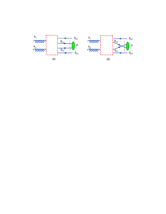
Figure 1: The schematic Feynman diagrams for the hadroproduction of $\Xi_{cc}$ from the gluon-gluon mechanism, where the dashed box stands for the hard interaction kernel. $k_{1}$ and $k_{2}$ are two momenta for the initial gluons, $q_{c2}$ and $q_{c4}$ are the momenta for the two outgoing $\bar{c}$, $P$ is the momentum of $\Xi_{cc}$. The $(cc)$-diquark pair is either in $(cc)_{\bf\bar{3}}[^{3}S_{1}]$ or in $(cc)_{\bf 6}[^{1}S_{0}]$ respectively.

The schematic Feynman diagrams for the gluon-gluon fusion mechanism are shown in Fig.(1). Fig.(1) shows that there are two ways for the two outgoing valence $c$ quarks to form the $(cc)$-diquark pair and each way contains 36 Feynman diagrams that are similar to the case of hadronic production of $B_{c}$ (all the diagrams can be found in Ref.bcvegpy1 , and one only need to change all the $b$ quark line there to the $c$ quark line). However in Refs.baranov ; kiselev1 ; kiselev2 , only Fig.(1a) is considered and then only 36 Feynman diagrams have been taken into consideration. Since the contributions from the left and the right diagrams of Fig.(1) are the same and there is an $\left(\frac{1}{2}\right)$ factor for the square of the amplitude by taking into account the symmetry of the diquark wavefunction, so there is an overall factor ‘2’ for our total cross-sections in comparing with those in Refs.baranov ; kiselev1 ; kiselev2 . In the present paper, as a cross check of the results in Refs. baranov ; kiselev1 ; kiselev2 , we calculated it by using two different methods and made a cross check numerically between them. One method is to fully simplify the amplitude of the gluon-gluon fusion mechanism by using the improved helicity approach which was developed in case of the hadronic production of $B_{c}$ bcvegpy1 ; bcvegpy2 . More details of the calculation could be found in the appendix A. The other is to generate the Fortran program directly by the Feynman Diagram Calculation (FDC) programfdc , which is a Reduce and Fortran package to perform Feynman diagram calculation automatically. The detailed treatment method of $\Xi_{cc}$ in FDC could be found in appendix B.

Figure 2: Typical Feynman diagrams for the sub-processes induced by ‘intrinsic’ charm. The upper five of them are those for $g(p_{1})+c(p_{2})\to\Xi_{cc}(p_{3})+\bar{c}(p_{4})$ and the lower five are for $c(p_{1})+c(p_{2})\to\Xi_{cc}(p_{3})+g(p_{4})$ respectively. The $(cc)$-diquark pair is either in $(cc)_{\bf\bar{3}}[^{3}S_{1}]$ or in $(cc)_{\bf 6}[^{1}S_{0}]$ respectively.

For the ‘intrinsic’ charm mechanism, we need to consider the following sub-processes, $g+c\to\Xi_{cc}+\bar{c}$ and $c+\bar{c}\to\Xi_{cc}+g$, where the $(cc)$-diquark pair in $\Xi_{cc}$ is in $(cc)_{\bf\bar{3}}[^{3}S_{1}]$ or $(cc)_{\bf 6}[^{1}S_{0}]$, respectively. Similar to the case of gluon-gluon fusion mechanism, There is a symmetry factor ‘2’ for cross section. The typical Feynman diagrams are shown in Fig.(2). The final expression of the total square of amplitude is quit simple, and we adopt the FDC program fdc to obtain it directly.

We will calculate the ‘intrinsic’ charm mechanism within the GM-VFN scheme. In GM-VFN scheme, when one talks about the heavy quark components of PDFs, and takes into account of both ‘heavy quark mechanisms’ and the gluon-gluon fusion mechanism for the hadronic production, one has to solve the double counting problem: i.e. a full QCD evolved ‘heavy quark’ charm/bottom distribution functions, according to the Altarelli-Parisi equations, includes all the terms proportional to $\ln\left(\frac{\mu^{2}}{m^{2}_{Q}}\right)$ ($\mu$ the factorization scale and $m_{Q}$ the heavy quark mass); and some of them come from the gluon-gluon fusion mechanism, i.e., a few terms appear from the integration of the phase-space for the gluon-gluon fusion mechanism.

To be specific, according to Eq.(1), the inclusive $\Xi_{cc}$ hadronic production via ‘intrinsic charm mechanisms’ can be formulated as,

$$d\sigma=\sum_{ij}\int dx_{1}\int dx_{2}F^{i}_{H_{1}}(x_{1},\mu_{F})\times F^{j}_{H_{2}}(x_{2},\mu)d\hat{\sigma}_{ij\rightarrow\Xi_{cc}X}(x_{1},x_{2},\mu)\,,$$ (4)

where $i\neq j$ and $i,j=g,c$. Here, the heavy quark PDF $F^{c}_{H}(x,\mu)$ ($x=x_{1}$ or $x_{2}$, $H=H_{1}$ or $H_{2}$), should include a proper subtraction term $F^{c}_{H}(x,\mu)_{SUB}$ as is defined in Eq.(2) in order to avoid the double counting of $g+c\to\Xi_{cc}+g$ mechanism to the gluon-gluon fusion mechanism. $d\hat{\sigma}_{ij\rightarrow\Xi_{cc}}$ stands for the usual 2-to-2 differential cross-section,

$$d\hat{\sigma}_{ij\rightarrow\Xi_{cc}X}(x_{1},x_{2},\mu^{2})=\frac{(2\pi)^{4}|\overline{M}|^{2}}{4\sqrt{(p_{1}\cdot p_{2})^{2}-m_{1}^{2}m_{2}^{2}}}\prod_{i=3}^{4}\frac{d^{3}\mathbf{p}_{i}}{(2\pi)^{3}(2E_{i})}\delta\left(\sum_{i=3}^{4}p_{i}-p_{1}-p_{2}\right),$$ (5)

where $p_{1}$, $p_{2}$ are the corresponding momenta for the initial two partons and $p_{3}$, $p_{4}$ are the momenta for the final ones respectively. The average over the initial parton’s spins and colors and the sum over the initial and the final state’s spins and colors are absorbed into $|\overline{M}|^{2}$. All the expressions of $|\overline{M}|^{2}$, with all the mass effects being retained, are shown in the appendix B.

The phase space integration can be manipulated by adopting the routines RAMBOS rkw and VEGAS gpl , which is the same as that of the $B_{c}$ meson generator BCVEGPY bcvegpy1 ; bcvegpy2 .

III numerical checks

Before analyzing the properties for the hadronic production of $\Xi_{cc}$, we need to check the rightness of program for all the mechanisms, especially, we should be more careful for the most complicate gluon-gluon fusion mechanism.

First of all, all the programs are checked by examining the gauge invariance of the amplitude, i.e. the amplitude vanishes when the polarization vector of an initial/final gluon is substituted by the momentum vector of this gluon. Numerically, we find that the gauge invariance is guaranteed at the computer ability (double precision) for all these processes. Next, to make sure the rightness of our program for the gluon-gluon fusion mechanism, as mentioned before, the numerical results of our two programs agree with each other exactly.

Furthermore, we compared our numerical results for the gluon-gluon fusion mechanism with those in the literature by using the same input parameters as were stated in the corresponding references. To make a complete comparison with the results listed in Ref.baranov , we also calculate the partonic cross sections for the production of $\Xi_{bc}$ and $\Xi_{bb}$ through the subprocesses, $gg\to\Xi_{bc}+\bar{b}+\bar{c}$ with the $(bc)$-diquark in color-anti-triplet $[^{3}S_{1}]$ or $[^{1}S_{0}]$ state, and $gg\to\Xi_{bb}+\bar{b}+\bar{b}$ with the $(bb)$-diquark in color-anti-triplet $[^{3}S_{1}]$ state. The programs for the production of $\Xi_{bc}$ and $\Xi_{bb}$ can be easily obtained from the program for the case of $\Xi_{cc}$.

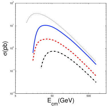
Figure 3: The energy dependence of the integrated partonic cross-section for the production of the baryons with heavy diquarks via the gluon-gluon fusion mechanism. The dotted line, solid line, dashed line and dash-dot line stand for the baryons with $(cc)_{\bf\bar{3}}[^{3}S_{1}]$, $(bc)_{\bf\bar{3}}[^{3}S_{1}]$, $(bc)_{\bf\bar{3}}[^{1}S_{0}]$ and $(bb)_{\bf\bar{3}}[^{3}S_{1}]$ respectively. The curves for $\Xi_{cc}$ and $\Xi_{bb}$ are divided by 2.

In Fig.(3), we show the partonic cross sections for the production of baryons with heavy diquarks via the gluon-gluon fusion subprocess. In drawing the curves, we adopt the same parameter values as were taken in Ref.baranov , i.e. with a fixed value for $\alpha_{s}$ ($\alpha_{s}=0.2$) and

$$|\Psi_{cc}(0)|^{2}=0.039GeV^{3},\;|\Psi_{bc}(0)|^{2}=0.065GeV^{3},\;|\Psi_{bb}(0)|^{2}=0.152GeV^{3}\ ,$$ (6)

$$m_{c}=1.8GeV,\;m_{b}=5.1GeV,\;M_{\Xi_{cc}}=3.6GeV,\;M_{\Xi_{bc}}=6.9GeV,\;M_{\Xi_{bb}}=10.2GeV\ .$$ (7)

For convenience of comparison with those of Ref.baranov , in Fig.(3), our results for $\Xi_{cc}$ and $\Xi_{bb}$ have been divided by an overall factor ‘2’. One may easily find all the curves for the energy dependence of the partonic cross-sections shown in Fig.(3) are in consistent with the results in Ref.baranov (Fig.(2a) there).

Table 1: Comparison of the partonic cross sections for $gg\rightarrow\Xi_{cc}+\bar{c}+\bar{c}$ with the corresponding results in Ref.kiselev1 , where the $(cc)$-diquark pair is in $(cc)_{\bf\bar{3}}[^{3}S_{1}]$. $E_{cm}$ is the center of mass energy of the subprocess. The input parameters are $m_{c}=1.7GeV$, $M_{\Xi_{cc}}=3.4GeV$, the radial wavefunction at the origin $R_{cc}(0)=\sqrt{4\pi}\Psi_{cc}(0)=0.601GeV^{3/2}$ and $\alpha_{s}=0.2$.

$E_{cm}$	15 GeV	20 GeV	40 GeV	60 GeV	80 GeV	100 GeV
$\sigma(pb)$	$66.6$	$68.2$	$41.8$	$26.2$	$17.9$	$13.1$
$\sigma(pb)$kiselev1	$23.2$	$22.5$	$13.7$	$8.96$	$6.45$	$4.94$

In Tab.(1), we show the comparison of partonic cross sections (the second column) for the production of $\Xi_{cc}$ with the $(cc)$-diquark in $(cc)_{\bf\bar{3}}[^{3}S_{1}]$ via the gluon-gluon fusion subprocess with those in Refs.kiselev1 ; kiselev2 . In Tab.(1), the results of Ref.kiselev1 is derived from the fitted expression (Eq.(8) in Ref.kiselev1 ):

$$\sigma=213.\left(1-\frac{4m_{c}}{E_{cm}}\right)^{1.9}\left(\frac{4m_{c}}{E_{cm}}\right)^{1.35},$$ (8)

where $E_{cm}$ is the center of mass energy of the subprocess. One may observe that under the same parameter values, the results in Refs.kiselev1 ; kiselev2 are in disagreement with ours even though they are close in shape .

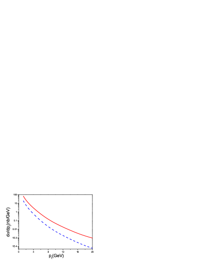
Figure 4: The $p_{t}$-distributions for the ‘intrinsic’ mechanism $c+c\to\Xi_{cc}+g$ at Tevatron RUN-I $E_{cm}=1.8$TeV (dashed line) or LHC $E_{cm}=14$TeV (solid line) both with $|y|\leq 1.0$. The present results are calculated with the same parameters in Ref. ref2 .

Next, as a cross-check between our results for one of the ‘intrinsic’ mechanism through $c+c\to\Xi_{cc}+g$ with those of Ref.ref2 , we show the cross section of $\Xi_{cc}$-baryon production at the hadronic energy $E_{cm}=1.8TeV$ or $14TeV$ with the same input parameters in Fig.(4). The curves in Fig.(4) agree with those of Ref.ref2 (Fig.3 and Fig.4 there).

As a summary, for the gluon-gluon fusion mechanism, except for an overall factor ‘2’, we confirm the results in Ref.baranov , but not those of Ref.kiselev1 ; kiselev2 . And for one of the ‘intrinsic’ charm mechanism, i.e. $c+c\to\Xi_{cc}+g$, our results agree with those of Ref.ref2 under the same input parameters.

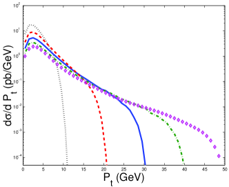
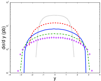
Figure 5: The $P_{t}-$ and $y-$distributions of the produced $\Xi_{cc}$ for the subprocess $gg\to\Xi_{cc}+\bar{c}+\bar{c}$ under different C.M. energies. Here the $(cc)$ diquark pair only in $(cc)_{\bf\bar{3}}[^{3}S_{1}]$ is taken into account. The dotted line, dashed line, solid line, dash-dot line and the diamond line stand for $E_{cm}=20$GeV, $40$GeV, $60$GeV, $80$GeV and $100$GeV, respectively.

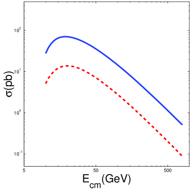
Figure 6: The energy dependence of the integrated partonic cross-section for the $\Xi_{cc}$ production of via the gluon-gluon fusion mechanism. The solid line and the dashed line stand for the two $(cc)$-diquark pair states in configurations $(cc)_{\bf\bar{3}}[^{3}S_{1}]$ and $(cc)_{\bf 6}[^{1}S_{0}]$ respectively.

Finally, we discuss the properties of the two different configurations of $(cc)$-diquark pair, i.e. $(cc)_{\bf\bar{3}}[^{3}S_{1}]$ and $(cc)_{\bf 6}[^{1}S_{0}]$, for the hadronic production of $\Xi_{cc}$. In Fig.(5), we show the transverse momentum $P_{t}$ distribution and the rapidity $y$ distribution at different center of mass energies for the subprocess $gg\to\Xi_{cc}+\bar{c}+\bar{c}$, with its $(cc)$-diquark pair in $(cc)_{\bf\bar{3}}[^{3}S_{1}]$. The case of $(cc)$-diquark pair in $(cc)_{\bf 6}[^{1}S_{0}]$ is similar and will not be shown here. We drawn a comparison between the energy dependence of the integrated partonic cross-section of the two different $(cc)$-diquark configurations, i.e. $(cc)_{\bf\bar{3}}[^{3}S_{1}]$ and $(cc)_{\bf 6}[^{1}S_{0}]$, in Fig.(6). One may observe that the curves for $(cc)_{\bf\bar{3}}[^{3}S_{1}]$ and $(cc)_{\bf 6}[^{1}S_{0}]$ are close in shape and the contributions from $(cc)_{\bf 6}[^{1}S_{0}]$ can be up to $\sim 20\%$ comparing with the case of $(cc)_{\bf\bar{3}}[^{3}S_{1}]$. So the contributions from the $(cc)$-diquark pair $(cc)_{\bf 6}[^{1}S_{0}]$ are significant and should be taken into consideration for a full estimation of the hadronic production of $\Xi_{cc}$. This is in agreement with the conclusion drawn in Ref.majp , where the contributions of these two different states of $(cc)$-diquark pair are discussed through the fragmentation approach.

IV hadronic production of $\Xi_{cc}$

In the present section, we shall first study the hadronic production properties of $\Xi_{cc}$ both at TEVATRON and at LHC, and then make a discussion for the hadronic production at the fixed target SELEX experiment. All the calculations are done under the GM-VFN scheme.

IV.1 hadronic production of $\Xi_{cc}$ at LHC and TEVATRON

As has been discussed in Sec.II, we take $h_{3}=|\Psi_{cc}(0)|^{2}$ and $h_{1}=h_{3}$ in the calculations. The mass of $M_{\Xi_{cc}}$ can be determined by potential model, and it is estimated to bekiselev1 , $M_{\Xi_{cc}}=3.584\pm 0.035GeV$. In Ref.exp , it has been measured to be $3.519\pm 0.001GeV$. For clarity, we choose $|\Psi_{cc}(0)|^{2}=0.039GeV^{3}$baranov , $M_{\Xi_{cc}}=3.50GeV$ and then $m_{c}=1.75GeV$. The factorization energy scale is fixed to be the transverse mass of $\Xi_{cc}$, i.e. $Q=M_{t}\equiv\sqrt{M^{2}+p_{t}^{2}}$, where $p_{t}$ is the transverse momentum of the baryon. The PDFs of version CTEQ6HQ 6hqcteq and the leading order $\alpha_{s}$ running above $\Lambda^{(n_{f}=4)}_{QCD}=0.326GeV$ are adopted.

Table 2: Cross sections $\sigma$ for the hadronic production of $\Xi_{cc}$ at TEVATRON and LHC, where the $(cc)$-diquark is in $(cc)_{\bf\bar{3}}[^{3}S_{1}]$ or $(cc)_{\bf 6}[^{1}S_{0}]$, and the symbol $g+c$ means $g+c\to\Xi_{cc}+\bar{c}$ and etc. In the calculations, $p_{t}\geq 4GeV$ is taken and $|y|\leq 1.5$ at LHC, while $|y|\leq 0.6$ at TEVATRON.

-	TEVATRON ($\sqrt{S}=1.96$ TeV)		LHC ($\sqrt{S}=14.0$ TeV)
-	$(cc)_{\bf\bar{3}}[^{3}S_{1}]$	$(cc)_{\bf 6}[^{1}S_{0}]$	$(cc)_{\bf\bar{3}}[^{3}S_{1}]$	$(cc)_{\bf 6}[^{1}S_{0}]$
$\sigma_{g+g}(nb)$	$1.61$	$0.392$	$22.3$	$5.44$
$\sigma_{c+g}(nb)$	$2.29$	$0.360$	$22.1$	$3.42$
$\sigma_{c+c}(nb)$	$0.751$	$0.0431$	$8.74$	$0.475$

In TABLE 2, we show the cross-section for the hadronic production of $\Xi_{cc}$ at TEVATRON and LHC, where $p_{t}\geq 4GeV$ is taken in the calculations and $|y|\leq 1.5$ at LHC, $|y|\leq 0.6$ at TEVATRON. From Tab.2, one may observe that similar to the case of hadronic production of $B_{c}$ meson zqww , the cross-sections of the ‘intrinsic’ charm mechanisms are comparable to, or even bigger than, the usual considered gluon-gluon fusion mechanism. From Tab.2, one may also observe that the contributions from $(cc)_{\bf 6}[^{1}S_{0}]$ are sizable comparing with that of $(cc)_{\bf\bar{3}}[^{3}S_{1}]$, i.e. for the gluon-gluon fusion mechanism, the contribution from $(cc)_{\bf 6}[^{1}S_{0}]$ is about $24\%$ of that of $(cc)_{\bf\bar{3}}[^{3}S_{1}]$, while for the mechanisms of $c+g\to\Xi_{cc}+\bar{c}$ and $c+c\to\Xi_{cc}+g$, it changes to $\sim 15\%$ and $\sim 5\%$, respectively.

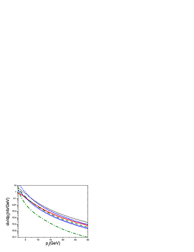
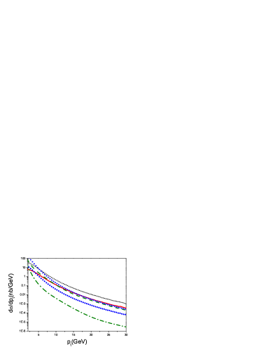
Figure 7: The $p_{t}$-distribution for the hadroproduction of $\Xi_{cc}$ at TEVATRON (left) and at LHC (right), where $|y|\leq 1.5$ at LHC and $|y|\leq 0.6$ at TEVATRON are adopted. The dotted line and the solid line are for gluon-gluon fusion mechanism, the triangle line and the diamond line are for $g+c\to\Xi_{cc}$, the dashed line and the dash-dot line are for $c+c\to\Xi_{cc}$, where the upper lines of each mechanism are for $(cc)_{\bf\bar{3}}[^{3}S_{1}]$ and the lower lines are for $(cc)_{\bf 6}[^{1}S_{0}]$, respectively.

In Fig.(7), we show $p_{t}$ distributions for the hadronic production of $\Xi_{cc}$ with two configurations of the $(cc)$-diquark pair states, i.e. $(cc)_{\bf\bar{3}}[^{3}S_{1}]$ and $(cc)_{\bf 6}[^{1}S_{0}]$, where $|y|\leq 1.5$ at LHC and $|y|\leq 0.6$ at TEVATRON are adopted. From Fig.(7), one may observe the following points: 1) to compare with the gluon-gluon fusion mechanism, the ‘intrinsic’ mechanism $g+c\to\Xi_{cc}+g$ dominant in small $p_{t}$ regions and its $p_{t}$ distributions drop faster than that of gluon-gluon fusion mechanism, which is similar to the case of $B_{c}$ hadroproduction zqww . 2) For ‘intrinsic’ mechanism $c+c\to\Xi_{cc}+g$, it $p_{t}$-distribution drops faster than other mechanisms and then its contribution is the smallest among all the mechanisms. 3) For a particular mechanism, the contribution from the case of $(cc)_{\bf 6}[^{1}S_{0}]$ is sizable comparing with the contribution from the case of $(cc)_{\bf\bar{3}}[^{3}S_{1}]$. However, the $p_{t}$ distribution of $(cc)_{\bf 6}[^{1}S_{0}]$ is smaller than that of $(cc)_{\bf\bar{3}}[^{3}S_{1}]$ in the whole $p_{t}$ regions for the same mechanism and it also drops faster than the case of $(cc)_{\bf\bar{3}}[^{3}S_{1}]$. Especially for the $c+c\to\Xi_{cc}$ mechanism, $p_{t}$ distribution of $(cc)_{\bf 6}[^{1}S_{0}]$ drop much faster than that of $(cc)_{\bf\bar{3}}[^{3}S_{1}]$, and then the cross-section for $(cc)_{\bf 6}[^{1}S_{0}]$ is only about $5\%$ of that of $(cc)_{\bf\bar{3}}[^{3}S_{1}]$. As for the gluon-gluon fusion mechanism, the contribution from $(cc)_{\bf 6}[^{1}S_{0}]$ is comparable to that of $(cc)_{\bf\bar{3}}[^{3}S_{1}]$ from the ‘intrinsic’ mechanisms at high energies, especially at LHC, so one should be careful to take the contribution from $(cc)_{\bf 6}[^{1}S_{0}]$ into consideration so as to provide a full estimation for all these hadronic mechanisms.

IV.2 A simple discussion on hadronic production of $\Xi_{cc}$ at the fixed target SELEX experiment

For the fixed target experiment, the ‘intrinsic’ charm mechanism becomes more important than in the case of hadronic production at TEVATRON or LHC, since small $p_{t}$ events can contribute here. Such an experiment has been done by SELEX group exp and it may cover all solid angle without $p_{t}$ cut, thus the ‘intrinsic’ charm mechanisms may be studied and extended to very small $p_{t}$ region. For SELEX experiment, its lower $p_{t}$ limit can be as small as $0.2GeV$. However, one should be careful to ensure that the pQCD calculation is reliable in such small $p_{t}$ regions, i.e. the intermediate gluon (with momentum $q$) in all the mechanisms for the hadronic production of $\Xi_{cc}$ must be hard enough, i.e. $q^{2}>>\Lambda_{QCD}^{2}$.

For the gluon-gluon fusion subprocess, the square of the intermediate gluon momentum at least is bigger than $(4m_{c}^{2})$ so as to produce one $c\bar{c}$-quark pair and then is always PQCD calculable. For the ‘intrinsic’ subprocess $g(p_{1})+c(p_{2})\to\Xi_{cc}(p_{3})+\bar{c}(p_{4})$, we must ensure that the momentum of the intermediate gluon of Fig.(2b,2c,2e) satisfy

$$Q^{2}=-q^{2}=-\left(p_{1}-\frac{p_{3}}{2}\right)^{2}>>\Lambda_{QCD}^{2}\;\;,$$ (9)

and for the ‘intrinsic’ subprocess $c(p_{1})+c(p_{2})\to\Xi_{cc}(p_{3})+g(p_{4})$, similarly, we have

$$Q^{2}_{1}=-q^{2}_{1}=-\left(p_{1}-\frac{p_{3}}{2}\right)^{2}>>\Lambda_{QCD}^{2}\,,\;\;\;\;\;\;Q^{2}_{2}=-q^{2}_{2}=-\left(p_{2}-\frac{p_{3}}{2}\right)^{2}>>\Lambda_{QCD}^{2}.$$ (10)

Eqs.(9,10) give two extra constraints for both the partonic fractions $x_{1}$, $x_{2}$ and $p_{t}$. For definiteness, we set the lowest values for $Q^{2}$, $Q^{2}_{1}$ and $Q^{2}_{2}$ to be $m_{c}^{2}$ ($>>\Lambda_{QCD}^{2}$).

Table 3: Cross section $\sigma$ for the hadronic production of $\Xi_{cc}$ at the fixed target experiment with center of mass energy $33.58GeV$, where the $(cc)$-diquark pair is in $(cc)_{\bf\bar{3}}[^{3}S_{1}]$ or $(cc)_{\bf 6}[^{1}S_{0}]$, and the symbol $g+c$ means $g+c\to\Xi_{cc}+\bar{c}$ and etc. In the calculations, $p_{t}>0.2GeV$ is taken.

-	SELEX ($\sqrt{S}=33.58$GeV)
-	$\sigma_{g+g}(pb)$	$\sigma_{g+c}(pb)$	$\sigma_{c+c}(pb)$
$(cc)_{\bf\bar{3}}[^{3}S_{1}]$	$4.03$	$102.$	$1.02\times 10^{-3}$
$(cc)_{\bf 6}[^{1}S_{0}]$	$0.754$	$11.3$	$4.15\times 10^{-5}$

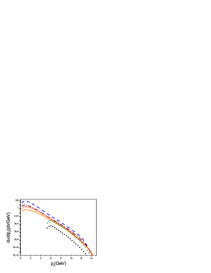
Figure 8: The $p_{t}$-distributions for the hadroproduction of $\Xi_{cc}$ at SELEX. The dotted line and the solid line are for gluon-gluon fusion mechanism, the dashed line and the dash-dot line are for $g+c\to\Xi_{cc}$, the triangle line and the diamond line are for $c+c\to\Xi_{cc}$, where the upper lines of each mechanism are for $(cc)_{\bf\bar{3}}[^{3}S_{1}]$ and the lower lines are for $(cc)_{\bf 6}[^{1}S_{0}]$, respectively.

We show the cross-section for the hadronic production of $\Xi_{cc}$ at SELEX experiment in TABLE 3, where $p_{t}>0.2GeV$ is adopted in the calculations. TABLE 3 shows that at SELEX, the ‘intrinsic’ charm mechanism is the dominant mechanism and then the theoretical predictions of $\Xi_{cc}$ events at SELEX can be raised by more than an order. We show the $p_{t}$ distributions for the fixed target experiment in Fig.(8). One may observe that the $p_{t}$ distributions of ‘intrinsic’ mechanism $g+c\to\Xi_{cc}+\bar{c}$ are bigger than that of the gluon-gluon fusion mechanism almost in all the $p_{t}$ region, which is the reason why the total cross-section of $g+c\to\Xi_{cc}+\bar{c}$ mechanism is much larger than the gluon-gluon fusion mechanism as shown in TABLE 3. For ‘intrinsic’ mechanism $c+c\to\Xi_{cc}+g$, it $p_{t}$-distribution starts at $\sim 5GeV$ due to the constraint Eq.(10) and its contribution is quite small. From TABLE 3, one may also observe that the contributions from $(cc)_{\bf 6}[^{1}S_{0}]$ are also sizable comparing with that of $(cc)_{\bf\bar{3}}[^{3}S_{1}]$ that is similar to the hadronic production at TEVATRON and LHC as shown in TABLE 2, i.e. for the gluon-gluon fusion mechanism, the contribution from $(cc)_{\bf 6}[^{1}S_{0}]$ is about $19\%$ of that of $(cc)_{\bf\bar{3}}[^{3}S_{1}]$, while for the processes of $c+g\to\Xi_{cc}+\bar{c}$ and $c+c\to\Xi_{cc}+g$, it changes to $\sim 10\%$ and $\sim 4\%$, respectively.

V summary

We have calculated the hadronic production of the doubly charmed baryon $\Xi_{cc}$ via the gluon-gluon fusion mechanism and the ‘intrinsic’ charm mechanism, i.e. via the sub-processes $g+g\to\Xi_{cc}+\cdots$, $g+c\to\Xi_{cc}+\cdots$ and $c+c\to\Xi_{cc}+\cdots$. To avoid the double counting problem while taking the gluon-gluon fusion mechanism and the ‘intrinsic’ charm mechanism into consideration, we have adopted the GM-VFN scheme in which the heavy-quark mass effects can be treated in a consistent way both for the hard scattering amplitude and the PDFs. Some cross checks for the present results with those in the literature have been done. The result for the gluon-gluon fusion mechanism agree with what was given in Ref.baranov up to a factor of 2; and the results for the $c+c\to\Xi_{cc}+g$ with $(cc)$-diquark pair in $cc_{\bf\bar{3}}[^{3}S_{1}]$ agree with that of Ref. ref2 when adopting the same input parameters. Whereas the results for the ‘intrinsic’ mechanisms and those for the cases with $(cc)$-diquark pair in $cc_{\bf 6}[^{1}S_{0}]$ are fresh.

Table 4: R values, which is defined in Eq.(11), for the hadronic production of $\Xi_{cc}$.

	SELEX	TEVATRON	LHC
-	$p_{t}>0.2GeV$	$p_{t}\geq 4GeV$, $|y|\leq 0.6$	$p_{t}\geq 4GeV$, $|y|\leq 1.5$
$R$	$29.$	$3.4$	$2.8$

From TABLE 2 and TABLE 3, one may see that the total cross sections of the ‘intrinsic’ charm mechanisms are comparable to, or even bigger than, that of the gluon-gluon fusion process, especially for the $g+c\to\Xi_{cc}$ mechanism. To be more definite, we define a ratio

$$R=\frac{\sigma_{total}}{\sigma_{gg\to\Xi_{cc}((cc)_{\bf\bar{3}}[^{3}S_{1}])}}\ ,$$ (11)

where $\sigma_{total}$ stands for the cross section for all the concerned mechanisms and $\sigma_{gg\to\Xi_{cc}((cc)_{\bf\bar{3}}[^{3}S_{1}])}$ is the cross section for the gluon-gluon fusion mechanism with $(cc)$-diquark pair in $(cc)_{\bf\bar{3}}[^{3}S_{1}]$ configuration only. The values of $R$ for the hadronic production of $\Xi_{cc}$ in various environments are shown in Tab.4, which shows that the ‘intrinsic’ charm mechanisms are not negligible: at SELEX they even dominate over the other mechanisms. The contributions from the $(cc)$-diquark pair in $cc_{\bf 6}[^{1}S_{0}]$ for all the concerned mechanisms are also considered in the work, and the results show that if the matrix element $h_{1}$ is at the same order of $h_{3}$ majp , i.e. $h_{1}\simeq h_{3}$, the diquark pair will make a sizable contribution to the hadronic production of $\Xi_{cc}$.

We may conclude that to be a full estimation for the hadronic production of $\Xi_{cc}$, one needs to take all these mechanisms into consideration. One may observe that by taking into account the ‘intrinsic’ mechanisms, the theoretical prediction on the $\Xi_{cc}$ event can be almost one order higher than the previous predictions in which only the gluon-gluon fusion mechanism is considered. Nevertheless, there is still a big discrepancy between the SELEX observation exp and pQCD predictions. Perhaps it is due to the fact that the small $p_{t}$ regions is not amenable to the pQCD analysis, e.g., the ‘intrinsic’ mechanism $c+c\to(cc)[^{3}S_{1}]_{\bf\bar{3}}+g$ and $c+c\to(cc)[^{1}S_{0}]_{\bf 6}+g$, according to constraint (10) there is a big contribution from non-perturbative QCD range, and the intrinsic charm fusion mechanism with the subprocesses $c+c\to(cc)[^{3}S_{1}]_{\bf\bar{3}}$ and $c+c\to(cc)[^{1}S_{0}]_{\bf 6}$, which may contribute to the production greatly but only with very small $p_{t}$, and being non-perturbative QCD nature, it is not considered here. Another possibility might be that the SELEX experiment does not provide sufficient support for its claim of evidence for the observation of doubly charmed baryon $\Xi_{cc}$ as pointed out by Ref.comm .

Acknowledgments: This work was supported in part by the Natural Science Foundation of China (NSFC).

Appendix A Calculation technology for the gluon-gluon fusion mechanism under the improved helicity approach

The general structure of the amplitude in ‘explicit helicity’ form can be written as

$$M_{i}^{(\lambda_{2},\lambda_{4},\lambda_{5},\lambda_{6})}(q_{c3},q_{c4},q_{c1},q_{c2},k_{1},k_{2}) = g_{s}^{4}\sum_{\lambda_{2},\lambda_{3}}C_{i}X_{i}D_{1}B_{Fi}^{(\lambda_{1},\lambda_{2},\lambda_{3},\lambda_{4},\lambda_{5},\lambda_{6})}(q_{c3},q_{c4},q_{c1},q_{c2},k_{1},k_{2})\cdot$$ (12)

$$D_{2}B_{(cc)}^{(\lambda_{1},\lambda_{3})}(q_{c3},q_{c1}),$$

where $i=1,\cdots,72$, $\lambda_{j}\;(j=1,\cdots,6)$ denote the helicities of the quarks and gluons respectively. $\lambda_{1}$ denotes the helicity of $c(q_{c3})$, $\lambda_{2}$ that of $\bar{c}(q_{c4})$, $\lambda_{3}$ that of $c(q_{c1})$, $\lambda_{4}$ that of $\bar{c}(q_{c2})$; whereas $\lambda_{5}$ denotes that of gluon-1 and $\lambda_{6}$ denotes that of gluon-2. Here $C_{i}$, $X_{i}$ denote the color factor and the scalar factor from all the propagators as a whole for the $i$th-diagram, respectively. $B_{Fi}^{(\lambda_{1},\lambda_{2},\lambda_{3},\lambda_{4},\lambda_{5},\lambda_{6})}(q_{c3},q_{c4},q_{c1},q_{c2},k_{1},k_{2})$ and $B_{(cc)}^{(\lambda_{1},\lambda_{3})}(q_{c3},q_{c1})$ are the amplitudes corresponding to the ‘free quark part’ $g(k_{1},\lambda_{5})g(k_{2},\lambda_{6})\rightarrow c(q_{c3},\lambda_{1})+\bar{c}(q_{c4},\lambda_{2})+c(q_{c1},\lambda_{3})+\bar{c}(q_{c2},\lambda_{4})$ (all the quarks are on-shell) and the ‘bound state part’ $c(q_{c3},\lambda_{1})+c(q_{c1},\lambda_{3})\rightarrow(cc)$, respectively. $D_{1}=\frac{1}{\sqrt{2q_{c3}\cdot q_{0}}}\frac{1}{\sqrt{2q_{c4}\cdot q_{0}}}\frac{1}{\sqrt{2q_{c1}\cdot q_{0}}}\frac{1}{\sqrt{2q_{c2}\cdot q_{0}}}$ and $D_{2}=\frac{1}{\sqrt{2q_{c1}\cdot q_{0}}}\frac{1}{\sqrt{2q_{c3}\cdot q_{0}}}$ are two common normalization factors.

By comparing Eq.(12) with Eq.(22) in Ref.bcvegpy1 that is for the $B_{c}$ hadroproduction, one may observe that both amplitudes are quite similar with each other. Most of the present helicity amplitudes can be directly derived from the results in Ref.bcvegpy1 by simply replacing the $b$-quark line there to the present $c$-quark line. And for the present case, we only need to deal with the following type of the helicity matrix element (HME) that is quite different from the case of $B_{c}$ hadroproduction, i.e.

$${\rm HME}_{i}=\langle q_{0\lambda_{2}}|(/\!\!\!q_{c4}+m_{c}){\bf\hat{\Gamma}_{i}}(/\!\!\!q_{c3}-m_{c})|q_{0\lambda_{1}}\rangle\ ,$$ (13)

where $i=(1,\cdots,72)$ stands for the $i$-th Feynman diagram and ${\bf\hat{\Gamma}_{i}}$ means that all the momentum in $\Gamma_{i}$ ($\Gamma_{i}$ stands for the explicit strings of Dirac $\gamma$ matrices between $\bar{U}(q_{c3})$ and $V(q_{c4})$, which corresponds to $i$-th Feynman diagram) should change their sign and the string of the $\gamma$-matrices in $\Gamma_{i}$ should be written in inverse order. In fact, such type of HME can also be relate to the familiar one as has been dealt with in the $B_{c}$ case by adopting the following relation:

$${\rm HME}_{i}=-\langle q_{0(-\lambda_{1})}|(/\!\!\!q_{c3}+m_{c})\Gamma_{i}(/\!\!\!q_{c4}-m_{c})|q_{0(-\lambda_{2})}\rangle\ .$$ (14)

A simple demonstration of Eq.(14) can be found in the last part of the appendix.

Table 5: The square of the six independent color factors (including the cross terms) for $gg\to(cc)_{\bf\bar{3}}[^{3}S_{1}]+\bar{c}+\bar{c}$, ($C_{mij}\times C_{nij}^{*}$) with $m,n=(1,2,\cdots,6)$, respectively.

	$C_{1ij}^{*}$	$C_{2ij}^{*}$	$C_{3ij}^{*}$	$C_{4ij}^{*}$	$C_{5ij}^{*}$	$C_{6ij}^{*}$
$C_{1ij}$	$\frac{4}{3}$	$-\frac{1}{6}$	$\frac{2}{3}$	$-\frac{1}{12}$	$\frac{5}{12}$	$-\frac{1}{3}$
$C_{2ij}$	$-\frac{1}{6}$	$\frac{4}{3}$	$-\frac{1}{12}$	$\frac{2}{3}$	$-\frac{1}{3}$	$\frac{5}{12}$
$C_{3ij}$	$\frac{2}{3}$	$-\frac{1}{12}$	$\frac{4}{3}$	$-\frac{5}{12}$	$\frac{1}{12}$	$-\frac{2}{3}$
$C_{4ij}$	$-\frac{1}{12}$	$\frac{2}{3}$	$-\frac{5}{12}$	$\frac{4}{3}$	$-\frac{2}{3}$	$\frac{1}{12}$
$C_{5ij}$	$\frac{5}{12}$	$-\frac{1}{3}$	$\frac{1}{12}$	$-\frac{2}{3}$	$\frac{4}{3}$	$-\frac{1}{6}$
$C_{6ij}$	$-\frac{1}{3}$	$\frac{5}{12}$	$-\frac{2}{3}$	$\frac{1}{12}$	$-\frac{1}{6}$	$\frac{4}{3}$

Table 6: The square of the six independent color factors (including the cross terms) for $gg\to(cc)_{\bf 6}[^{1}S_{0}]+\bar{c}+\bar{c}$, ($C_{mij}\times C_{nij}^{*}$) with $m,n=(1,2,\cdots,6)$, respectively.

	$C_{1ij}^{*}$	$C_{2ij}^{*}$	$C_{3ij}^{*}$	$C_{4ij}^{*}$	$C_{5ij}^{*}$	$C_{6ij}^{*}$
$C_{1ij}$	$\frac{8}{3}$	$-\frac{1}{3}$	$\frac{2}{3}$	$-\frac{1}{12}$	$\frac{11}{12}$	$\frac{1}{6}$
$C_{2ij}$	$-\frac{1}{3}$	$\frac{8}{3}$	$-\frac{1}{12}$	$\frac{2}{3}$	$\frac{1}{6}$	$\frac{11}{12}$
$C_{3ij}$	$\frac{2}{3}$	$-\frac{1}{12}$	$\frac{8}{3}$	$\frac{11}{12}$	$-\frac{1}{12}$	$\frac{2}{3}$
$C_{4ij}$	$-\frac{1}{12}$	$\frac{2}{3}$	$\frac{11}{12}$	$\frac{8}{3}$	$\frac{2}{3}$	$-\frac{1}{12}$
$C_{5ij}$	$\frac{11}{12}$	$\frac{1}{6}$	$-\frac{1}{12}$	$\frac{2}{3}$	$\frac{8}{3}$	$-\frac{1}{3}$
$C_{6ij}$	$\frac{1}{6}$	$\frac{11}{12}$	$\frac{2}{3}$	$-\frac{1}{12}$	$-\frac{1}{3}$	$\frac{8}{3}$

The sum of all the helicity amplitudes of the sub-process $g+g\to(cc)+\bar{c}+\bar{c}$ can be arranged as

$$M^{(\lambda_{2},\lambda_{4},\lambda_{5},\lambda_{6})}(q_{c3},q_{c4},q_{c1},q_{c2},k_{1},k_{2}) = \sum_{m=1}^{6}C_{mij}M^{(\lambda_{2},\lambda_{4},\lambda_{5},\lambda_{6})}_{m}(q_{c3},q_{c4},q_{c1},q_{c2},k_{1},k_{2})\;,$$ (15)

where $C_{mij}$ ($m=1-6$) are six independent color factors of the process,

$$C_{1ij} = \frac{1}{2\sqrt{2}}\left(T^{a}T^{b}\right)_{mi}G_{mjk}\;,\;\;C_{2ij}=\frac{1}{2\sqrt{2}}\left(T^{b}T^{a}\right)_{mi}G_{mjk}\;,$$

$$C_{3ij} = \frac{1}{2\sqrt{2}}(T^{a})_{mj}(T^{b})_{ni}G_{mnk}\;,\;\;C_{4ij}=\frac{1}{2\sqrt{2}}(T^{b})_{mj}(T^{a})_{ni}G_{mnk}\;,$$

$$C_{5ij} = \frac{1}{2\sqrt{2}}\left(T^{a}T^{b}\right)_{mj}G_{mik}\;,\;\;C_{6ij}=\frac{1}{2\sqrt{2}}\left(T^{b}T^{a}\right)_{mj}G_{mik}\;,$$ (16)

where $i,j=1,2,3$ are color indices of the two outgoing anti-quarks $\bar{c}$ and $\bar{c}$ respectively, and the indices $a$ and $b$ are color indices for gluon-1 and gluon-2 respectively. Here, the function $G_{mjk}$ equals to the anti-symmetric $\varepsilon_{mjk}$ for the $(cc)$-diquark in $\bf\bar{3}$ configuration and equals to the symmetric $f_{mjk}$ for the $(cc)$-diquark in $\bf 6$ configuration respectively. The anti-symmetric $\varepsilon_{mjk}$ satisfies $\varepsilon_{mjk}\varepsilon_{m^{\prime}j^{\prime}k}=\delta_{mm^{\prime}}\delta_{jj^{\prime}}-\delta_{mj^{\prime}}\delta_{jm^{\prime}}$ and the symmetric $f_{mjk}$ satisfies $f_{mjk}f_{m^{\prime}j^{\prime}k}=\delta_{mm^{\prime}}\delta_{jj^{\prime}}+\delta_{mj^{\prime}}\delta_{jm^{\prime}}$.

To get the matrix element squared, one needs to deal with the square of the above six independent color factors as shown in Eq.(16) (including the cross terms), i.e. ($C_{mij}\times C_{nij}^{*}$) with $m,n=(1,2,\cdots 6)$. For reference use, we list the square of these six independent color factors in TABLE 5 and TABLE 6, which are for $(cc)_{\bf\bar{3}}[^{3}S_{1}]$ and $(cc)_{\bf 6}[^{1}S_{0}]$, respectively.

By keeping all these points in mind, we rewrite a program based on the $B_{c}$ meson generator BCVEGPYbcvegpy1 ; bcvegpy2 to calculate the gluon-gluon fusion mechanism for the hadronic production of $\Xi_{cc}$.

Finally, we give a simple demonstration of the relation Eq.(14). To demonstrate the relation Eq.(14), we shall adopt the following relation,

$$\langle p_{(\lambda_{1})}|/\!\!\!k_{1}.../\!\!\!k_{n}|q_{(\lambda_{2})}\rangle=(-1)^{n+1}\langle q_{(-\lambda_{2})}|/\!\!\!k_{n}.../\!\!\!k_{1}|p_{(-\lambda_{1})}\rangle\ ,$$ (17)

whose non-zero ones can be explicitly written as zdl

$$\langle p_{-}|/\!\!\!k_{1}.../\!\!\!k_{n}|q_{+}\rangle = -\langle q_{-}|/\!\!\!k_{n}.../\!\!\!k_{1}|p_{+}\rangle\,\,\,(n\,\,\,even),$$ (18)

$$\langle p_{+}|/\!\!\!k_{1}.../\!\!\!k_{n}|q_{-}\rangle = -\langle q_{+}|/\!\!\!k_{n}.../\!\!\!k_{1}|p_{-}\rangle\,\,\,(n\,\,\,even),$$ (19)

$$\langle p_{+}|/\!\!\!k_{1}.../\!\!\!k_{n}|q_{+}\rangle = \langle q_{-}|/\!\!\!k_{n}.../\!\!\!k_{1}|p_{-}\rangle\,\,\,(n\,\,\,odd),$$ (20)

where $k_{i}(i=1,\cdots,n)$ are any types of momenta.

Generally, to the $i$-th Feynman diagram, we can expand $\Gamma_{i}$ as,

$$\Gamma_{i}=\sum_{n}C_{n}(\not{\!p}_{1}\not{\!p}_{2}\cdots\not{\!p}_{n}),$$ (21)

and then we have,

$${\bf\hat{\Gamma}_{i}}=\sum_{n}(-1)^{n}C_{n}(\not{\!p}_{n}\cdots\not{\!p}_{2}\not{\!p}_{1}),$$ (22)

where $C_{n}$ are functions free of Dirac $\gamma$ matrix element. Taking use of Eq.(17), we finally obtain

$$\langle q_{0(-\lambda_{1})}|(/\!\!\!q_{c3}+m_{c})\Gamma_{2i}(/\!\!\!q_{c4}-m_{c})|q_{0(-\lambda_{2})}\rangle$$ (23)

$$= \sum_{n}C_{n}\langle q_{0(-\lambda_{1})}|\left[\not{\!q}_{c3}(\not{\!p}_{1}\not{\!p}_{2}\cdots\not{\!p}_{n})\not{\!q}_{c4}-m_{c}\not{\!q}_{c3}(\not{\!p}_{1}\not{\!p}_{2}\cdots\not{\!p}_{n})\right.$$

$$\quad\quad\quad\quad\quad\quad\quad+\left.m_{c}(\not{\!p}_{1}\not{\!p}_{2}\cdots\not{\!p}_{n})\not{\!q}_{c4}-m_{c}^{2}(\not{\!p}_{1}\not{\!p}_{2}\cdots\not{\!p}_{n})\right]|q_{0(-\lambda_{2})}\rangle$$

$$= \sum_{n}C_{n}\langle q_{0(\lambda_{2})}|\left[(-1)^{n+3}\not{\!q}_{c4}(\not{\!p}_{n}\cdots\not{\!p}_{2}\not{\!p}_{1})\not{\!q}_{c3}-(-1)^{n+2}m_{c}(\not{\!p}_{n}\cdots\not{\!p}_{2}\not{\!p}_{1})\not{\!q}_{c3}\right.$$

$$\quad\quad\quad\quad\quad+\left.(-1)^{n+2}m_{c}\not{\!q}_{c4}(\not{\!p}_{n}\cdots\not{\!p}_{2}\not{\!p}_{1})-(-1)^{n+1}m_{c}^{2}(\not{\!p}_{n}\cdots\not{\!p}_{2}\not{\!p}_{1})\right]|q_{0(\lambda_{1})}\rangle$$

$$= -\langle q_{0(\lambda_{2})}|(/\!\!\!q_{c4}+m_{c}){\bf\hat{\Gamma}_{2i}}(/\!\!\!q_{c3}-m_{c})|q_{0(\lambda_{1})}\rangle.$$

Appendix B calculation technology in FDC programfdc and the square of amplitude for the intrinsic charm mechanism

First, we take gluon-gluon fusion mechanism as an explicit example to show the technology used in FDC programfdc and show in more detail how we can derive the program for the hadronic production of $\Xi_{cc}$ from those of $J/\psi$.

The amplitude for each Feynman diagram of $g+g\to J/\psi(p_{3})+c(p_{4})+{\bar{c}}(p_{5})$ can be written as:

$$M(J/\psi)= {\bar{u}(p_{4},s_{4})}\Gamma_{1}s_{f}(k_{1},m_{c})\cdots s_{f}(k_{n-1},m_{c})\Gamma_{n}v(\displaystyle{p_{3}\over 2},s_{1})$$ (24)

$$B(p_{3},s,s_{1},s_{2},m_{J/\psi}){\bar{u}(\displaystyle{p_{3}\over 2},s_{2})}\Gamma^{\prime}_{1}s_{f}(q_{1},m_{c})\cdots s_{f}(q_{n^{\prime}-1})\Gamma^{\prime}_{n^{\prime}}v(p_{5},s_{5}).$$

where $s_{f}(k,m)$ ($k=k_{i}$ or $q_{i}$) is the fermion propagator, $B(p_{3},s,s_{1},s_{2},m_{J/\psi})$ is the wavefunction of $J/\psi$, $\Gamma_{1},\cdots,\Gamma_{n},\Gamma^{\prime}_{1},\cdots,\Gamma^{\prime}_{n},$ are the interaction vertices. The color factor part is treated separately (similar to the method described in Appendix.A) and will not discussed here.

One can easily find out the corresponding Feynman diagram in $g+g\to\Xi_{cc}(p_{3})+{\bar{c}}(p_{4})+{\bar{c}}(p_{5})$ and the amplitude of it could be written as:

$$M(\Xi_{cc})= {\bar{u}(\displaystyle{p_{3}\over 2},s_{1})}\Gamma_{n}s_{f}(-k_{n-1},m_{c})\cdots s_{f}(-k_{1},m_{c})\Gamma_{1}v(p_{4},s_{4})$$ (25)

$$B(p3,s,s_{1},s_{2},m_{\Xi_{cc}}){\bar{u}(\displaystyle{p_{3}\over 2},s_{2})}\Gamma^{\prime}_{1}s_{f}(q_{1},m_{c})\cdots s_{f}(q_{n^{\prime}-1},m_{c})\Gamma^{\prime}_{n^{\prime}}v(p_{5},s_{5}),$$

where $B(p_{3},s,s_{1},s_{2},m_{\Xi_{cc}})$ is the wavefunction of $\Xi_{cc}$. For an arbitrary Fermion line,

$$a={\bar{u}(\displaystyle{p_{3}\over 2},s_{1})}\Gamma_{n}s_{f}(-k_{n-1},m_{c})\cdots s_{f}(-k_{1},m_{c})\Gamma_{1}v(p_{4},s_{4}),$$

we have

$$a=a^{T}=v^{T}(p_{4},s_{4})\Gamma^{T}_{1}s^{T}_{f}(-k_{1},m_{c})\cdots s^{T}_{f}(-k_{n-1},m_{c})\Gamma^{T}_{n}{\bar{u}(\displaystyle{p_{3}\over 2},s_{1})}^{T}$$

$$=v^{T}(p_{4},s_{4})CC^{-}\Gamma^{T}_{1}CC^{-}s^{T}_{f}(-k_{1},m_{c})CC^{-}\cdots CC^{-}s^{T}_{f}(-k_{n-1},m_{c})CC^{-}\Gamma^{T}_{n}CC^{-}{\bar{u}(\displaystyle{p_{3}\over 2},s_{1})}^{T}$$

$$=(-1)^{(n+1)}{\bar{u}(p_{4},s_{4})}\Gamma_{1}s_{f}(k_{1},m_{c})\cdots s_{f}(k_{n-1},m_{c})\Gamma_{n}v(\displaystyle{p_{3}\over 2},s_{1}),$$

with the help of the following equations

$$v^{T}(p_{4},s_{4})C=-{\bar{u}(p_{4},s_{4})},~{}~{} C^{-}{\bar{u}({p_{3}\over 2},s_{1})}^{T}=v({p_{3}\over 2},s_{1}),~{}~{}$$

$$C^{-}\Gamma^{T}_{i}C=-\Gamma_{i},~{}~{} C^{-}s^{T}_{f}(-k_{i},m_{c})C=s_{f}(k_{i},m_{c}).$$

Where $C=-i\gamma^{2}\gamma^{0}$ is the charge conjugation matrix. And then Eq.(25) can be transformed as

$$M(\Xi_{cc})= (-1)^{(n+1)}{\bar{u}(p_{4},s_{4})}\Gamma_{1}s_{f}(k_{1},m_{c})\cdots s_{f}(k_{n-1},m_{c})\Gamma_{n}v(\displaystyle{p_{3}\over 2},s_{1})$$ (26)

$$B(p_{3},s,s_{1},s_{2},m_{\Xi_{cc}}){\bar{u}(\displaystyle{p_{3}\over 2},s_{2})}\Gamma^{\prime}_{1}s_{f}(q_{1},m_{c})\cdots s_{f}(q_{n^{\prime}-1})\Gamma^{\prime}_{n^{\prime}}v(p_{5},s_{5}).$$

By comparing Eq.(24) with Eq.(26), one find that they are the same except for an overall factor $(-1)^{(n+1)}$, where ‘$n$’ is the interaction vertex number of the corresponding fermion line and depends on the detail of each Feynman diagram. Therefore, we can completely use the method of $J/\psi$ to deal with $\Xi_{cc}$ case by adding a factor $(-1)^{(n+1)}$ diagram by diagram. The detailed description of method to treat the $J/\psi$ and $B_{c}$ calculation could be found in the Ref.fdc ; bcvegpy2 .

All the above discussion is also valid for the calculation of the ‘intrinsic’ charm mechanisms. And the following results are obtained by taking the FDC program.

For convenience, we express the square of the amplitudes by the variants $s$, $t$ and $u$, which are defined as:

$$s=(p_{1}+p_{2})^{2},~{}~{}~{}t=(p_{1}-p_{3})^{2},~{}~{}~{}u=(p_{1}-p_{4})^{2},$$

where $p_{i}=(E_{i},p_{ix},p_{iy},p_{iz})$ are the corresponding momenta for the involved particles: $p_{1}$ and $p_{2}$ are the momenta of initial partons, $p_{3}$ and $p_{4}$ are the momenta of $\Xi_{cc}$ and another outgoing particles respectively. Further more, for $\bar{c}(p_{1})+g(p_{2})\to\Xi_{cc}(p_{3})+\bar{c}(p_{4})$, we set

$$u_{1}=(u-4m_{c}^{2}),~{}~{}~{}s_{1}=(s-m_{c}^{2}),~{}~{}~{}t_{1}=(t-m_{c}^{2}),$$

and for $c(p_{1})+c(p_{2})\to\Xi_{cc}(p_{3})+g(p_{4})$, we set

$$u_{1}=(u-m_{c}^{2}),~{}~{}~{}s_{1}=(s-4m_{c}^{2}),~{}~{}~{}t_{1}=(t-m_{c}^{2}).$$

The relation, $u_{1}+t_{1}+s_{1}=0$, is useful to make all the expressions for the square of the amplitudes compact.

The square of the amplitude for the subprocess $c(p_{1})+g(p_{2})\to\Xi_{cc}(p_{3})+\bar{c}(p_{4})$ with $(cc)$-diquark pair in $(cc)_{\bf\bar{3}}[^{3}S_{1}]$ can be written as,

$$|\overline{M}|^{2} = {2^{9}{\alpha_{s}}^{3}|\Psi_{cc}(0)|^{2}{\pi}^{4}\over 3^{5}{M}}\left[4M^{2}\left({10\over u_{1}^{2}}+{-4\over s_{1}t_{1}}+{11u_{1}^{2}\over s_{1}^{2}t_{1}^{2}}+{4u_{1}^{4}\over s_{1}^{3}t_{1}^{3}}\right)+4M^{4}\left({-17\over s_{1}t_{1}u_{1}}+{28u_{1}\over s_{1}^{2}t_{1}^{2}}+{-20u_{1}^{3}\over s_{1}^{3}t_{1}^{3}}\right)\right.$$ (27)

$$\left.+3M^{6}\left({-12\over s_{1}t_{1}u_{1}^{2}}+{-5\over s_{1}^{2}t_{1}^{2}}+{-14u_{1}^{2}\over s_{1}^{3}t_{1}^{3}}+{4u_{1}^{4}\over s_{1}^{4}t_{1}^{4}}\right)+8\left({-2\over u_{1}}+{11u_{1}\over s_{1}t_{1}}+{-9u_{1}^{3}\over s_{1}^{2}t_{1}^{2}}\right)\right].$$

The square of the amplitude for the subprocess $c(p_{1})+g(p_{2})\to\Xi_{cc}(p_{3})+\bar{c}(p_{4})$ with $(cc)$-diquark pair in $(cc)_{\bf 6}[^{1}S_{0}]$ can be written as,

$$|\overline{M}|^{2} = {2^{9}{\alpha_{s}}^{3}|\Psi_{cc}(0)|^{2}{\pi}^{4}\over 3^{5}{M}}\left[M^{2}\left({-20\over u_{1}^{2}}+{-1\over s_{1}t_{1}}+{-12u_{1}^{2}\over s_{1}^{2}t_{1}^{2}}\right)+4M^{4}\left({-12\over s_{1}t_{1}u_{1}}+{-u_{1}\over s_{1}^{2}t_{1}^{2}}+{-2u_{1}^{3}\over s_{1}^{3}t_{1}^{3}}\right)\right.$$ (28)

$$\left.+M^{6}\left({-48\over s_{1}t_{1}u_{1}^{2}}+{8\over s_{1}^{2}t_{1}^{2}}+{-7u_{1}^{2}\over s_{1}^{3}t_{1}^{3}}+{2u_{1}^{4}\over s_{1}^{4}t_{1}^{4}}\right)+2\left({-10\over u_{1}}+{9u_{1}\over s_{1}t_{1}}+{-2u_{1}^{3}\over s_{1}^{2}t_{1}^{2}}\right)\right].$$

The square of the amplitude for the subprocess $c(p_{1})+c(p_{2})\to\Xi_{cc}(p_{3})+g(p_{4})$ with $(cc)$-diquark pair in $(cc)_{\bf\bar{3}}[^{3}S_{1}]$ can be written as,

$$|\overline{M}|^{2} = {2^{11}{\alpha_{s}}^{3}|\Psi_{cc}(0)|^{2}{\pi}^{4}\over 3^{6}{M}}\left[4M^{2}\left({-4s_{1}^{4}\over t_{1}^{3}u_{1}^{3}}+{11s_{1}^{3}\over t_{1}^{2}u_{1}^{3}}+{15s_{1}^{2}\over t_{1}u_{1}^{3}}+{18s_{1}\over u_{1}^{3}}+{34t_{1}\over u_{1}^{3}}+{30t_{1}^{2}\over s_{1}u_{1}^{3}}+{10t_{1}^{3}\over s_{1}^{2}u_{1}^{3}}\right)\right.$$ (29)

$$\left.+4M^{4}\left({20s_{1}^{3}\over t_{1}^{3}u_{1}^{3}}+{28s_{1}^{2}\over t_{1}^{2}u_{1}^{3}}+{28s_{1}\over t_{1}u_{1}^{3}}+{17\over s_{1}t_{1}u_{1}}\right)+3M^{6}\left({-4s_{1}^{4}\over t_{1}^{4}u_{1}^{4}}+{-14s_{1}^{3}\over t_{1}^{3}u_{1}^{4}}+{-9s_{1}^{2}\over t_{1}^{2}u_{1}^{4}}+{-2s_{1}\over t_{1}u_{1}^{4}}\right.\right.$$

$$\left.\left.+{-31\over u_{1}^{4}}+{-36t_{1}\over s_{1}u_{1}^{4}}+{-12t_{1}^{2}\over s_{1}^{2}u_{1}^{4}}\right)+8\left({9s_{1}^{3}\over t_{1}^{2}u_{1}^{2}}+{11s_{1}^{2}\over t_{1}u_{1}^{2}}+{11s_{1}\over u_{1}^{2}}+{2\over s_{1}}\right)\right].$$

The square of the amplitude for the subprocess $c(p_{1})+c(p_{2})\to\Xi_{cc}(p_{3})+g(p_{4})$ with $(cc)$-diquark pair in $(cc)_{\bf 6}[^{1}S_{0}]$ can be written as,

$$|\overline{M}|^{2} = {2^{11}{\alpha_{s}}^{3}|\Psi_{cc}(0)|^{2}{\pi}^{4}\over 3^{6}{M}}\left[M^{2}\left({12s_{1}^{2}\over t_{1}^{2}u_{1}^{2}}+{-s_{1}\over t_{1}u_{1}^{2}}+{-1\over u_{1}^{2}}+{20\over s_{1}^{2}}\right)+4M^{4}\left({2s_{1}^{3}\over t_{1}^{3}u_{1}^{3}}+{-s_{1}^{2}\over t_{1}^{2}u_{1}^{3}}+{-s_{1}\over t_{1}u_{1}^{3}}+\right.\right.$$ (30)

$$\left.\left.{12\over s_{1}t_{1}u_{1}}\right)+M^{6}\left({-2s_{1}^{4}\over t_{1}^{4}u_{1}^{4}}+{-7s_{1}^{3}\over t_{1}^{3}u_{1}^{4}}+{-15s_{1}^{2}\over t_{1}^{2}u_{1}^{4}}+{-64s_{1}\over t_{1}u_{1}^{4}}+{-152\over u_{1}^{4}}+{-144t_{1}\over s_{1}u_{1}^{4}}+{-48t_{1}^{2}\over s_{1}^{2}u_{1}^{4}}\right)+\right.$$

$$\left.2\left({2s_{1}^{3}\over t_{1}^{2}u_{1}^{2}}+{9s_{1}^{2}\over t_{1}u_{1}^{2}}+{9s_{1}\over u_{1}^{2}}+{10\over s_{1}}\right)\right].$$

In these equation, $M$ is the mass of $\Xi_{cc}$ and $\Psi_{cc}(0)$ is the wavefunction at origin for the $[^{3}S_{1}]$ $cc$ state. And here we have adopted that $h_{3}=|\Psi_{cc}(0)|^{2}$ and $h_{1}=h_{3}$.

References

- (1) M. Mattson et al., SELEX Collaboration, Phys. Rev. Lett. 89, 112001(2002).
- (2) A. Ocherashvili et al., SELEX Collaboration, hep-ex/0406033.
- (3) V.V. Kiselev and A.K. Likhoded, hep-ph/0208231.
- (4) M. Moinester, Z.Phys. A355, 349(1996); V.V. Kiselev and A. Likhoded, hep-ph/0103169.
- (5) S.P. Baranov, Phys. Rev. D54, 3228(1996).
- (6) A.V. Berezhnoy, V.V. Kiselev, A.K. Likhoded and A.I. Onishchenko, Phys. Rev. D57, 4385(1998).
- (7) A.V. Berezhnoy, V.V. Kiselev and A.K. Likhoded, Phys.Atom.Nucl. 59, 870(1996).
- (8) A.V. Berezhnoy, V.V. Kiselev and A.K. Likhoded, Sov. J. Nucl. Phys. 59, 909(1996).
- (9) J.P. Ma and Z.G. Si, Phys. Lett. B568, 135(2003).
- (10) G.T. Bodwin, E. Braaten, and G.P. Lepage, Phys. Rev. D51, 1125 (1995); Erratum:ibid., D55, 5853 (1997).
- (11) Cong-Feng Qiao, J. Phys. G29, 1075(2003); hep-ph/0202227.
- (12) Chao-Hsi Chang, Cong-Feng Qiao, Jian-Xiong Wang and Xing-Gang Wu, Phys. Rev. D 72, 114009(2005).
- (13) F.I. Olness, R.J. Scalise and W.T. Tung, Phy. Rev. D59, 014506(1998).
- (14) M.A.G. Aivazis, J.C. Collins, F.I. Olness and W.K. Tung, Phys. Rev. D50, 3102(1994); Phys. Rev. D50, 3085(1994).
- (15) J. Amundson, C. Schmidt, W.K. Tung and X.N. Wang, JHEP10, 031(2000).
- (16) S. Kretzer, H.L. Lai, F.I. Olness and W.K. Tung, Phys. Rev. D69, 114005(2004).
- (17) M. Klasen, B.A. Kniehl, L.N. Mihaila and M. Steihauser, Phys. Rev. Lett. 89, 032001(2002); Chao-Hsi Chang and Xing-Gang Wu, Eur. Phys. J. C38, 267(2004); Chao-Hsi Chang, Jian-Xiong Wang and Xing-Gang Wu, Phys. Rev. D70, 114019(2004); N. Brambilla et al., hep-ph/0412158.
- (18) Chao-Hsi Chang, Chafik Driouich, Paula Eerola and Xing-Gang Wu, Comput. Phys. Commun. 159, 192(2004).
- (19) Chao-Hsi Chang, Jian-Xiong Wang and Xing-Gang Wu, hep-ph/0504017, to be published in Comput. Phys. Commun..
- (20) Jian-Xiong Wang, Nucl. Instrum. Methods Phys. Res., Sect. A 534, 241 (2004).
- (21) D.A. Günter and V.A. Saleev, Phys. Rev. D64, 034006(2001).
- (22) R. Kleiss and W.J. Stirling, Comput. Phys. Commun, 40 (1986) 359.
- (23) G.P. Lepage, J. Comp. Phys 27 (1978) 192.
- (24) J. Collins, F. Wilczek and A. Zee, Phys. Rev. D18, 242 (1978).
- (25) Zhan Xu, Da-Hua Zhang and Lee Chang, Nucl. Phys. 291, 392 (1987).