Abstract

A broad overview of the current status of proton stability in unified models of particle interactions is given which includes non - supersymmetric unification, SUSY and SUGRA unified models, unification based on extra dimensions, and string-M-theory models. The extra dimensional unification includes 5D and 6D and universal extra dimensional (UED) models, and models based on warped geometry. Proton stability in a wide array of string theory and M theory models is reviewed. These include Calabi-Yau models, grand unified models with Kac-Moody levels $k>1$, a new class of heterotic string models, models based on intersecting D branes, and string landscape models. The destabilizing effect of quantum gravity on the proton is discussed. The possibility of testing grand unified models, models based on extra dimensions and string-M-theory models via their distinctive modes is investigated. The proposed next generation proton decay experiments, HyperK, UNO, MEMPHYS, ICARUS, LANNDD (DUSEL), and LENA would shed significant light on the nature of unification complementary to the physics at the LHC. Mathematical tools for the computation of proton lifetime are given in the appendices. Prospects for the future are discussed.

in

Grand Unified Theories,

in Strings and in Branes

Pran Nath¹, and Pavel Fileviez Pérez²

¹ Department of Physics. Northeastern University
Boston, MA 02115, USA.
email:nath@lepton.neu.edu

² Departamento de Física. Centro de Física Teórica de Partículas,
Instituto Superior Técnico, Av. Rovisco Pais 1, 1049-001.
Lisboa, Portugal.
email:fileviez@cftp.ist.utl.pt

1 Introduction

The Standard Model of strong, and the electro-weak interactions, given by the gauge group $SU(3)_{C}\times SU(2)_{L}\times U(1)_{Y}$, is a highly successful model of particle interactions [1, 2] which has been tested with great accuracy by the LEP, SLC and Tevatron data. The electro-weak sector of this theory [1], i.e., the $SU(2)_{L}\times U(1)_{Y}$ sector, provides a fundamental explanation of the Fermi constant and the scale

$$G_{F}^{-\frac{1}{2}}\simeq 292.8{\rm GeV}$$ (1)

has its origin in the spontaneous breaking of the $SU(2)_{L}\times U(1)_{Y}$ gauge group and can be understood as arising from the vacuum expectation value ($v$) of the Higgs boson field ($H^{0}$) so that $G_{F}^{-\frac{1}{2}}=2^{1/4}v$. Thus the scale $G_{F}$ is associate with new physics, i.e., the unification of the electro-weak interactions. There are at least two more scales which are associated with new physics. First, from the high precision LEP data, one finds that the gauge coupling constants $g_{3},g_{2},g_{1}(=\sqrt{\frac{5}{3}}g_{Y})$, where $g_{3},g_{2},g_{Y}$ are the gauge coupling constants for the gauge groups $SU(3)_{C}$, $SU(2)_{L}$, $U(1)_{Y}$, appear to unify within the minimal supersymmetric standard model at a scale $M_{G}$ so that

$$M_{G}\simeq 2\times 10^{16}~{}{\rm GeV}$$ (2)

This scale which is presented here as empirical must also be associated with new physics. A candidate theory here is grand unification. Finally, one has the Planck scale defined by

$$M_{\rm Pl}=(8\pi G_{N})^{-\frac{1}{2}}\simeq 2.4\times 10^{18}~{}{\rm GeV}$$ (3)

where one expects physics to be described by quantum gravity, of which string-M-theory are possible candidates. Quite remarkable is the fact that the scale $M_{G}$ where the gauge couping unification occurs is smaller than the Planck scale by about two orders of magnitude. This fact has important implications in that one can build a field theoretic description of unification of particle interactions without necessarily having a full solution to the problem of quantum gravity which operates at the scale $M_{\rm Pl}$. Since grand unified theories and models based on strings typically put quarks and leptons in common multiplets their unification in general leads to proton decay, and thus proton stability becomes one of the crucial tests of such models. Recent experiments have made such limits very stringent, and one expects that the next generation of experiments will improve the lower limits by a factor of ten or more. Such an improvement may lead to confirmation of proton decay which would then provide us with an important window to the nature of the underlying unified structure of matter. Even if no proton decay signal is seen, we will have much stronger lower limits than what the current experiment gives, which would constrain the unified models even more stringently. This report is timely since many new developments have occurred since the early eighties. On the theoretical side there have been developments such as supersymmetry and supergravity grand unification, and model building in string, in D branes, and in extra dimensional framework. On the experimental side Super-Kamiokande has put the most stringent lower limits thus far on the proton decay partial life times. Further, we stand at the point where new proton decay experiments are being planned. Thus it appears appropriate at this time to present a broad view of the current status of unification with proton stability as its focus. This is precisely the purpose of this report.

We give now a brief description of the content of the report. In Sec.(2) we review the current status of proton decay lower limits from recent experiments. The most stringent limits come from the Super-Kamiokande experiment. We also describe briefly the proposed future experiments. These new generation of experiments are expected to increase the lower limits roughly by a factor of ten. In Sec.(3) we discuss proton stability in non-supersymmetric scenarios. In Sec.3.1 we estimate the proton lifetime where the B -violating effective operators are induced by instantons. In Sec.(3.2) we discuss the baryon and lepton number violating dimension six operators induced by gauge interactions which are $SU(3)_{C}\times SU(2)_{L}\times U(1)_{Y}$ invariant. Proton decay modes from these $B-L$ preserving interactions are also discussed. In Sec.(3.3), we discuss the general set of dimension six operators induced by scalar lepto-quarks consistent with $SU(3)_{C}\times SU(2)_{L}\times U(1)_{Y}$ interactions.

In Sec.(4) nucleon decay in supersymmetric gauge theories is discussed. In Sec.(4.1) the constraint on R parity violating interactions to suppress rapid proton decay from baryon and lepton number  violating dimension four operators is analyzed. However, in general proton decay from baryon and lepton number  violating dimension five operators will occur and in this case it is the most dominant contribution to proton decay in most of the supersymmetric grand unified theories. The analysis of proton decay dimension five operators requires that one convert the baryon and lepton number  violating dimension five operators by chargino, gluino and neutralino exchanges to convert them to baryon and lepton number  violating dimension six operators. The dressing loop diagrams depend sensitively on soft breaking. Thus in Sec.(4.2) a brief review of supersymmetry breaking is given. As is well known, the soft breaking sector of supersymmetric theories depends on CP phases and thus the dressing loop diagrams and proton decay can be affected by the presence of such phases. A discussion of this phenomenon is given in Sec.(4.3). Typically in grand unified theories the Higgs iso-doublets with quantum numbers of the MSSM Higgs fields and the Higgs color- triplets are unified in a single representation. Since we need a pair of light Higgs iso-doublets to break the electro-weak symmetry, while we need the Higgs triplets to be heavy to avoid too fast a proton decay, a doublet-triplet splitting is essential for any viable unified model. Sec.(4.4) is devoted to this important topic. The remainder of Sec.(4) is devoted to a discussion of proton decay in specific models. A discussion of proton decay in $SU(5)$ grand unification is given in Sec.(4.5), while a discussion of proton decay in $SO(10)$ models is given in Sec.(4.6). In Sec.(4.7) a new $SO(10)$ framework is given where a single constrained vector-spinor - a 144- multiplet is used to break $SO(10)$ down to the residual gauge group symmetry $SU(3)_{C}\times U(1)_{em}$.

Sec.(5) is devoted to tests of grand unification through proton decay and a number of items that impinge on it are discussed. One of these concerns the implication of Yukawa textures on the proton lifetime. It is generally believed that the fermion mass hierarchy may be more easily understood in terms of Yukawa textures at a high scale and there are many proposals for the nature of such textures. It turns out that the Higgs triplet textures are not the same as the Higgs doublet textures, and a unified framework allows for the calculation of such textures. This topic is discussed in Sec.(5.1). Supergravity grand unification involves three arbitrary functions: the superpotential, the Kahler potential, and the gauge kinetic energy function. Non-universalities in gauge kinetic energy function can affect both the gauge coupling unification and proton lifetime. This topic is discussed in Sec.(5.2). In grand unified models, the gauge coupling unification receives threshold corrections from the low mass (sparticle) spectrum as well from the high scale (GUT) masses. Consequently the GUT scale masses, and specifically the Higgs triplet mass, are constrained by the high precision LEP data. These constraints are discussed in Sec.(5.3). Model independent tests of distinguishing GUT models using meson and anti-neutrino final state are discussed in Sec.(5.4) where three different models, $SU(5)$, flipped $SU(5)$ and $SO(10)$ are considered. In Sec(5.5) the important issue of the constraints necessary to rotate away or eliminate the baryon and lepton number  violating dimension six operators induced by gauge interactions is discussed. It is shown that it is possible to satisfy such constraints for the flipped $SU(5)$ case. Finally, an analysis of the upper limits on the proton lifetime on baryon and lepton number  violating dimension six operators induced by gauge interactions is given in Sec.(5.6).

Sec.(6) is devoted to grand unified models in extra dimensions and the status of proton stability in such models. In Sec.(6.1) a discussion of proton stability in grand unified models in dimension five (i.e., with one extra dimension) is given and various possibilities where the matter could reside either on the branes or in the bulk are discussed. In these models it is possible to get a natural doublet-triplet splitting in the Higgs sector with no Higgs triplets and anti-triples with zero modes. A review of $SO(10)$ models in 5D is given in Sec.(6.2) while 5D trinification models are discussed in Sec.(6.3). 6D grand unification models in dimension six, i.e., on $R\times T^{2}$, are discussed in Sec.(6.4). Various grand unification possibilities on the branes, i.e., $SO(10)$, $SU(5)\times U(1)$, flipped $SU(5)\times U(1)$, and $SU(4)_{C}\times SU(2)_{L}\times SU(2)_{R}$ exist in this case. Another class of models which are closely related to the models above are those with gauge-Higgs unification. Here the Higgs fields arise as part of the gauge multiplet and hence gauge and Higgs couplings are unified. Various possibilities for the suppression of proton decay exist in these models since proton decay is sensitive to how matter is located in extra dimensions. In Sec.(6.6) a discussion of proton decay in models with universal extra dimensions (UED) is given. In these models extra symmetries arise which can be used to control proton decay. In Sec.(6.7) proton stability in models with warped geometry is discussed. Such models lead to a solution to the hierarchy problem via a warp factor which depends on the extra dimension. Proton decay can be suppressed through a symmetry which conserves baryon number. Finally, in Sec.(6.8) proton stability in kink backgrounds is discussed.

In Sec.(7) we discuss proton stability in string and brane models. There are currently five different types of string theories: Type I, Type IIA, Type IIB, SO(32) heterotic and $E_{8}\times E_{8}$ heterotic. These are all connected by a web of dualities and conjectured to be subsumed in a more fundamental M-theory. Realistic and semi-realistic model building has been carried out in many of them and most extensive investigations exist for the case of the $E_{8}\times E_{8}$ heterotic string within the so called Calabi-Yau compactifications where the effective group structure after Wilson line breaking is $SU(3)_{C}\times SU(3)_{L}\times SU(3)_{R}$ and further breaking through the Higgs mechanism is needed to break the group down to the Standard Model gauge group. Proton stability in Calabi-Yau models is discussed in Sec.(7.1). In Sec.(7.2) we discuss grand unification in Kac-Moody levels $k>1$. It is known that in weakly coupled heterotic strings one cannot realize massless scalars in the adjoint representation at level 1, and one needs to go to levels $k>1$ to realize massless scalars in the adjoint representations necessary to break the GUT symmetry. However, at level 2 it is difficult to obtain 3 massless generations while this problem is overcome at level 3. In these models baryon and lepton number violating dimension four operators are absent due to an underlying gauge and discrete symmetry. However, baryon and lepton number  violating dimension five operators are present and one needs to suppress them by heavy Higgs triplets. A detailed analysis of proton lifetime in these models is currently difficult due the problem of generating proper quark-lepton masses. In Sec.(7.3) a new class of heterotic string models are discussed which have the interesting feature that they have the spectrum of MSSM, while proton decay is absolutely forbidden in these models, aside from the proton decay induced by quantum gravity effects. Other attempts at realistic model building in 4D models in the heterotic string framework are also briefly discussed in Sec.(7.3).

Proton decay in M-theory compactifications are discussed in Sec.(7.4). The low energy limit of this theory is the 11 dimensional supergravity theory and one can preserve $N=1$ supersymmetry if one compactifies the 11 dimensional supergravity on a seven-compact manifold X of $G_{2}$ holonomy. The manifold X can be chosen to give non-abelian gauge symmetry and chiral fermion. Currently quantitative predictions of proton lifetime do not exist due to an unknown overall normalization factor which requires an M theory calculation for its computation. However, it is still possible to make qualitative predictions in this theory. Thus for a class of X-manifolds, baryon and lepton number  violating dimension five operators are absent but baryon and lepton number  violating dimension six operators do exist and here one can make the interesting prediction that the decay mode $p\to e^{+}_{R}\pi^{0}$ is suppressed relative to the mode $p\to e^{+}_{L}\pi^{0}$. In Sec(7.5) proton decay in intersecting D brane models is discussed. Here we consider proton decay in $SU(5)$ like GUT models in Type IIA orientifolds with D-6 branes. It is assumed that the baryon and lepton number  violating dimension 4 and dimension 5 operators are absent and that the observable proton decay arises from dimension six operators. The predictions of the model here may lie within reach of the next generation of proton decay experiment. In Sec.(7.6) we discuss proton stability in string landscape models. There are a variety of scenarios in this class of models where the squarks and sleptons can be very heavy and thus proton decay via dimension five operators will be suppressed. Such is the situation on the so called Hyperbolic Branch of radiative breaking of the electro-weak symmetry. A brief review is given in Sec.(7.6) of the possible scenarios within string models where a hierarchical breaking of supersymmetry can occur. In Sec.(7.7) a review of proton decay from quantum gravity effects is given. It is conjectured that quantum gravity does not conserve baryon number and thus can catalyze proton decay. Thus, for example, quantum gravity effects could induce baryon number violating processes of the type $qq\to\bar{q}l$. Proton decay via quantum gravity effects in the context of large extra dimensions are also discussed in Sec.(7.7). In Sec.(7.8) a discussion of $U(1)$ string symmetries is given which allow the suppression of proton decay from dimension four and dimension five operators. In Sec.(7.9) discrete symmetries for the suppression of proton decay are discussed. However, if the discrete symmetries are global they are not respected by quantum gravity specifically, for example, in virtual black hole exchange and in wormhole tunneling. However, gauged discrete symmetries allows one to overcome this hurdle. A brief discussion of the classification of such symmetries is also given in Sec.(7.9).

A number of other topics related to proton stability in GUTs, strings and branes are discussed in Sec.(8). Thus an interesting issue concerns the connection between proton stability and neutrino masses. This connection is especially relevant in the context of grand unified models based on $SO(10)$ and the discussion of Sec.(8.1) is devoted to this case. Supersymmetric models with R parity invariance lead to the lowest supersymmetric particle (LSP) being absolutely stable. In supergravity GUT models the LSP over much of the parameter space turns out to be the lightest neutralino. Thus supersymmetry/supergravity models provide a candidate for cold dark matter. The recent WMAP data puts stringent constraints on the amount of dark matter. The dark matter constraints have a direct bearing on predictions of the proton lifetime in unified models. This topic is discussed in Sec.(8.2). In Sec.(8.3) exotic baryon and lepton number  violation is discussed. These include processes involving $\Delta B=3$ such as ${}^{3}H\to e^{+}\pi^{0}$, baryon and lepton number  violation involving higher generations, e.g., $p\to\tau^{*}\to\bar{\nu}_{\tau}\pi^{+}$, and proton decay via monopole catalysis where $M+p\to M+e^{+}+{\rm mesons}$. Finally, Sec.(8.4) contains speculations on proton decay and the ultimate fate of the universe. Sec.(9) contains a summary of the report highlighting some of the important elements of the report and outlook for the future.

Many of the mathematical details of the report are relegated to the Appendices. Thus in Appendix A mathematical aspects of the grand unification groups $SU(5)$ and $SO(10)$ necessary for understanding the discussion in the main text are given. In Appendix B, the allowed contributions arising from dimension five operators to proton decay are listed. In Appendix C a glossary of dressings of dimension five operators by chargino, gluino, and neutralino exchanges is given. The dressing loop diagrams involve sparticle masses, and in Appendix D an analysis of the sparticle spectra at low energy using renormalization group is given. Appendix E is devoted to a discussion of the renormalization group factors of the dimension 5 and dimension 6 operators. A detailed discussion of the effective Lagrangian which allows one to convert baryon and lepton number  violating quark-lepton dimension six operator to interactions involving baryons and mesons is given in Appendix F. Appendix G gives details of the analysis of testing models, and Appendix H gives the details on the analysis of upper bounds. Appendix I gives a discussion of how one may relate the 4D parameters to the parameters of M theory. Finally, Appendix J is devoted to a discussion of the gauge coupling unification in string and D brane models.

2 Experimental bounds and future searches

The issue of proton stability has attracted attention over three quarters of a century. Thus in the period 1929-1949 the law of baryon number conservation was formulated by Weyl, Stueckelberg and Wigner [3], and the first experimental test of the idea was proposed by Maurice Goldhaber in 1954 [4, 5]. The basic idea of Goldhaber was that nucleon decay could leave $Th^{232}$ in an excited and fissionable state, and thus comparison of the measured lifetime to that for spontaneous fission could be used to search for nucleon decay. This technique produced a lower limit on the proton lifetime of $\tau>1.4\times 10^{18}$ years. The first direct search for proton decay was made by F. Reines, C. Cowan and M. Goldhaber [6] using a 300 liter liquid scintillation detector, and they set a limit on the lifetime of free protons of $\tau>1\times 10^{21}$ years and a lifetime for bound nucleons of $\tau>1\times 10^{22}$ years. From a theoretical view point the idea that proton may be unstable originates in the work on Sakharov in 1967 [7] who postulated that an explanation of baryon asymmetry in the universe requires CP violation and baryon number non-conservation. Further, impetus for proton decay came with the work of Pati and Salam in 1973 [8] and later with non-supersymmetric [9, 10], supersymmetric [11], and supergravity [12, 13] grand unification, and from quantum gravity where black hole and worm hole effects can catalyze proton decay [14, 15, 16, 17, 18].

Thus spurred by theoretical developments in the nineteen seventies and the eighties there were large scale experiments for the detection of proton decay. Chief among these are the Kolar Gold Field[19], NUSEX [20], FREJUS [21], SOUDAN [22], Irvine-Michigan-Brookhaven (IMB)[23] and Kamiokande [24]. These experiments use either tracking calorimeters (e.g. SOUDAN) or Cherenkov effect (IMB, Kamiokande). These experiments yielded null results but produced improved lower bounds on various proton decay modes. In the nineteen nineties the largest proton water Cherenkov detector, Super-Kamiokande, came on line for the purpose of searching for proton decay and for the study of the solar and atmospheric neutrino properties. Super-Kamiokande [25] is a ring imaging water Cherenkov detector containing 50 ktons of ultra pure water held in a cylindrical stainless steel tank 1 km underground in a mine in the Japanese Alps. The sensitive volume of water is split into two parts. The 2 m thick outer detector is viewed with 1885 20 cm diameter photomultiplier tubes. When relativistic particles pass through the water they emit Cherenkov light at an angle of about $42^{0}$ from the particle direction of travel. By measuring the charge produced in each photo multiplier tube and the time at which it is collected, it is possible to reconstruct the position and energy of the event as well as the number, identity and momenta of the individual charged particles in the event.

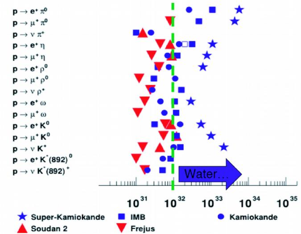
Figure 4: Experimental lower bounds on proton decay partial lifetimes [34]

The progress in the last 50 years of proton decay searches is shown in Figure 4, where the experimental lower bounds for the partial proton decay lifetimes are exhibited. The plot exhibits the power of the water Cerenkov detectors in improving the proton decay lower bounds. Since Super-kamiokande is currently the most sensitive proton decay experiment, it is instructive to examine briefly the signatures of proton decay signals in this experiment. We focus on the decay mode $p\to e^{+}\pi^{0}$. Since it is one of the simplest modes it serves well as a general example of proton decay searches.

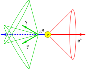
Figure 1: Idealized $p\to e^{+}\pi^{0}$ decay in Super-Kamiokande [26].

Fig.(1) gives a schematic presentation of an ideal $p\to e^{+}\pi^{0}$ decay. Here, the positron, $e^{+}$ and neutral pion $\pi^{0}$, exit the decay region in opposite directions. The positron initiates an electromagnetic shower leading to a single isolated ring. The $\pi^{0}$ will almost immediately decay to two photons which will go on to initiate showers creating two, usually overlapping, rings. In general, real $p\to e^{+}\pi^{0}$ events will differ from this ideal picture because the pion can scatter or be absorbed entirely before it exits the nucleus. In addition the proton in the nucleus can have some momentum due to Fermi motion. These two effects, i.e., the pion-nucleon interaction and Fermi motion, serve to spoil the balance of the reconstructed momentum. Further, the pion can decay asymmetrically where one photon takes more than half of the pion’s energy leaving the second photon to create a faint or even completely invisible ring. All these effects are taken into account in search for proton decay signals. Super-Kamiokande experiment also searches for the $p\to K^{+}\bar{\nu}$ mode by looking for the products from the two primary branches of the $K^{+}$ decay (see Figure 2). In the $K^{+}\to\mu^{+}\nu_{\mu}$ case, when the decaying proton is in the ${}^{16}O$, the nucleus will be left as an excited ¹⁵N. Upon de-excitation, a prompt 6.3 MeV photon will be emitted (See Figure 3).

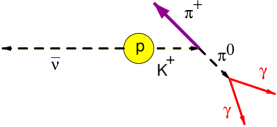
Figure 2: Idealized $p\to K^{+}\nu$ decay in Super-Kamiokande, $K^{+}\to\pi^{+}\pi^{0}$ case [26]

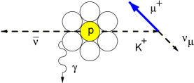
Figure 3: Idealized $p\to K^{+}\nu$ decay in Super-Kamiokande, $K^{+}\to\mu^{+}\nu_{\mu}$ case [26]

An important question for proton decay searches concerns the issue of backgrounds. There are three classes of atmospheric neutrino background events that are directly relevant for proton decay searches. The first is the inelastic charged current events, $\nu N\to N^{\textasciiacute}{e,\mu}+n\pi$, where a neutrino interacts with a nucleon in the water and produces a visible lepton and a number of pion’s. This can mimic proton decay modes such as $p\to e^{+}\pi^{0}$. The second class is neutral current pion production, $\nu N\to\nu N^{\textasciiacute}n\pi$, the only visible products of which are pion’s. This is the background to, for example, $n\to\nu\eta$. Finally, there are quasi elastic charged current events $\nu N\to N^{\textasciiacute}{\mu,e}$, events which can look like, $p\to K^{+}\bar{\nu}$. The current experimental lower bounds on proton decay lifetimes are listed in Table 1.

We note that presently the largest lower bound is for the mode $p\to e^{+}\pi^{0}$. Interestingly the radiative decay modes $p\to e^{+}\gamma$ and $p\to\mu^{+}\gamma$ also have very strong constraints.

Channel	$\tau_{p}$ ($10^{30}$ years)
$p\to invisible$	0.21
$p\to e^{+}\pi^{0}$	1600
$p\to\mu^{+}\pi^{0}$	473
$p\to\nu\pi^{+}$	25
$p\to e^{+}\eta^{0}$	313
$p\to\mu^{+}\eta^{0}$	126
$p\to e^{+}\rho^{0}$	75
$p\to\mu^{+}\rho^{0}$	110
$p\to\nu\rho^{+}$	162
$p\to e^{+}\omega^{0}$	107
$p\to\mu^{+}\omega^{0}$	117
$p\to e^{+}K^{0}$	150
$p\to e^{+}K^{0}_{S}$	120
$p\to e^{+}K^{0}_{L}$	51
$p\to\mu^{+}K^{0}$	120
$p\to\mu^{+}K^{0}_{S}$	150
$p\to\mu^{+}K^{0}_{L}$	83
$p\to\nu K^{+}$	670
$p\to e^{+}K^{*}(892)$	84
$p\to\nu K^{*}(892)$	51
$p\to e^{+}\gamma$	670
$p\to\mu^{+}\gamma$	478

Table 1: Experimental lower bounds on proton lifetimes  [27]. The limits listed are on $\tau/B_{i}$, where $\tau$ is the total mean life and $B_{i}$ is the branching fraction for the relevant mode.

Recently the Super-Kamiokande collaboration has reported new experimental lower bounds on proton decay lifetimes. The improved limits for some of the channels are as follows [28]:

$$\tau(p\to K^{+}\bar{\nu})\ > \ 2.3\times 10^{33}\ \textrm{years}$$ (4)

$$\tau(p\to K^{0}\mu^{+})\ > \ 1.3\times 10^{33}\ \textrm{years}$$ (5)

$$\tau(p\to K^{0}e^{+})\ > \ 1.0\times 10^{33}\ \textrm{years}$$ (6)

As will be discussed later in this report, proton decay is a probe of fundamental interactions at extremely short distances and as such it is an instrument for the exploration of grand unifications, of Planck scale physics and of quantum gravity and more specifically of string theory and M theory. For this reason it is crucial to have new experiments to search for proton decay or improve the current bounds. Fortunately, there are several proposals currently under discussion. Thus several new experiments have been proposed based mainly on two techniques: the usual water Cherenkov detector and the use of noble gases, the Liquid Argon Time Projection Chamber (LAr TPC). The proposed future experiments based on the water Cherenkov detector are: the one-megaton HYPERK [29, 30], the UNO experiment [31] with a 650 kt of water, while the experiment 3M [32] is proposed with a 1000 kt and the European megaton project MEMPHYS at Frejus [33].

On the other hand the ICARUS experiment [34] is based on the Liquid Argon Time Projection Chamber (LAr TPC) technique. A more ambitious proposal along similar lines for proton decay and neutrino oscillation study (LANNDD) is a 100 kT liquid Argon TPC which is proposed for the Deep Underground Science and Engineering Laboratory (DUSEL) in USA [35]. Yet another proposal is of a Low Energy Neutrino Astronomy (LENA) detector consisting of a 50 kt of liquid scintillator [36]. The LENA detector is suitable for SUSY favored decay channel $p\to\bar{\nu}K^{+}$ where the kaon will cause a prompt mono-energetic signal while the neutrino escapes without producing any detectable signal. It is estimated that within ten years of measuring time a lower limit of $\tau>4\times 10^{34}$ years can be reached [36]. Basically all those proposals together with Super-Kamiokande define the next generation of proton decay experiments. These experiments will either find proton decay or at the very least improve significantly the lower bounds and eliminate many models. Thus, for example, the goal of Hyper-Kamiokande is to explore the proton lifetime at least up to $\tau_{p}/B(p\to e^{+}\pi^{0})>10^{35}$ years and $\tau_{p}/B(p\to K^{+}\bar{\nu})>10^{34}$ years in a period of about 10 years [30]. Thus the next generation of proton decay experiments mark an important step to probe the structure of matter at distances which fall outside the realm of any current or future accelerator.

3 Nucleon decay in non-supersymmetric scenarios

As mentioned in Sec.(2) proton decay is a generic prediction of grand unified theories. There are different operators contributing to the nucleon decay in such theories. In supersymmetric scenarios the $d=4$ and $d=5$ contributions are the most important, but quite model dependent. They depend on the whole SUSY spectrum, on the structure of the Higgs sector and on fermion masses. The so-called gauge $d=6$ contributions for proton decay are the most important in non-supersymmetric grand unified theories, which basically depend only on fermion mixing. The remaining Higgs $d=6$ operators coming from the Higgs sector are less important and they are quite model dependent, since we can have different structures in the Higgs sector. In this section we will study the stability of the proton in the Standard Model, and the nucleon decay induced by the super-heavy gauge and Higgs bosons. The outline of the rest of this section is as follows: In Sec. (3.1) we discuss the B -violating effective operators induced by instantons and estimate the proton lifetime arising from them. An analysis of $SU(3)_{C}\times SU(2)_{L}\times U(1)_{Y}$ invariant and $B-L$ preserving baryon and lepton number violating dimension six operators induced by gauge interactions is given in Sec.(3.2). Also discussed are the proton decay modes from these interactions. $SU(3)_{C}\times SU(2)_{L}\times U(1)_{Y}$ baryon and lepton number -violating dimension six operators can also be induced by scalar lepto-quark exchange and an analysis of these is given in Sec.(3.3). We give below the details of these analyzes.

3.1 Baryon number violation in the Standard Model

The Standard Model with gauge symmetry $SU(3)_{C}\ \times SU(2)_{L}\ \times U(1)_{Y}$ has a $U(1)_{B}$ global symmetry at the classical level, where $B$ is the baryon number, which implies stability of the lightest baryon, i.e., the proton, in the universe. However, this global symmetry is broken at the quantum level by anomalies [37], i.e. the baryonic current $J^{\mu}_{B}$ is not conserved:

$$\partial_{\mu}J^{\mu}_{B}=\frac{n_{f}g^{2}}{16\pi^{2}}TrF_{\mu\nu}\tilde{F}^{\mu\nu}$$ (7)

where $n_{f}$ is the number of generations and

$$F_{\mu\nu}=\partial_{\mu}A_{\nu}-\partial_{\nu}A_{\mu}-ig[A_{\mu},A_{\nu}]$$ (8)

while

$$\tilde{F}_{\mu\nu}=\frac{1}{2}\epsilon_{\mu\nu\alpha\beta}\ F^{\alpha\beta}$$ (9)

With the above anomaly baryon number violation can arise from instanton transitions between degenerate $SU(2)_{L}$ gauge vacua. The B-violating effective operator induced by the instanton processes is given by (for details see, for example, [38]):

$$O_{eff}=c(\frac{1}{M_{W}})^{14}e^{-\frac{2\pi}{\alpha_{2}}}\prod_{i=1}^{3}(\ \epsilon_{\alpha\beta\gamma}\ Q_{\alpha L}^{i}\ Q_{\beta L}^{i}\ Q_{\gamma L}^{i}\ L_{L}^{i})$$ (10)

where i is the generation index. The above interaction leads to violations of baryon and lepton number so that $\Delta B=\Delta L=3$. We note, however, the front factor would give a rate so that

$${\rm Rate}\sim|e^{-\frac{2\pi}{\alpha_{2}}}|^{2}\sim 10^{-173}$$ (11)

Clearly this is a highly suppressed rate irrespective of other particulars. However, baryon and lepton number violating dimension six and higher operators can be written consistent with the Standard Model gauge invariance.  [39, 40, 41]. This is the subject of discussion in the remainder of this section.

3.2 Grand unification and gauge contributions to the decay of the proton

We discuss now a unifying framework beyond that of the Standard Model. There are many reasons for doing so. One of the major ones is the presence of far too many arbitrary parameters in the Standard Model and it is difficult to accept that a fundamental theory should be that arbitrary. One example of this is the presence of three independent gauge couplings: $\alpha_{s}$ for the color interactions, $\alpha_{2}$ for $SU(2)_{L}$, and $\alpha_{Y}$ for the gauge group $U(1)_{Y}$. This arbitrariness could be removed if one had a semi-simple gauge group, i.e., a grand unified group, with a single gauge coupling constant. Thus the three gauge coupling constants will be unified in such a scheme at a high scale, but would be split at low energy due to their different renormalization group evolution from the grand unification scale to low scales. Of course, the correctness of a specific assumption of grand unification must be tested by a detailed comparison of the predictions of the unified model with the precision LEP data on the couplings. Another virtue of grand unification is that it leads to an understanding of the quantization of charge, e.g., $|Q_{e}|=|Q_{p}|$, while such an explanation is missing in the Standard Model. Additionally, grand unification reduces arbitrariness in the Yukawa coupling sector, by relating Yukawa couplings for particles that reside in the common multiplets. However, one important consequence of grand unification as noted earlier is that it leads generically to proton decay. This arises from the fact that in grand unified models quarks and leptons fall in common multiplets and thus interactions lead to processes involving violations of baryon and lepton number.

In this subsection we focus on the non-supersymmetric contributions to the decay of the proton (For an early review of proton decay in non-supersymmetric grand unification see Ref. [42]). In particular we study the gauge $d=6$ operators. Using the properties of the Standard Model fields we can write down the possible $d=6$ operators contributing to the decay of the proton, which are $SU(3)_{C}\times SU(2)_{L}\times U(1)_{Y}$ invariant [39, 40, 41]:

$$\textit{O}^{B-L}_{I} = k^{2}_{1}\ \epsilon_{ijk}\ \epsilon_{\alpha\beta}\ \overline{u_{ia}^{C}}_{L}\ \gamma^{\mu}\ {Q_{j\alpha a}}_{L}\ \overline{e_{b}^{C}}_{L}\ \gamma_{\mu}\ {Q_{k\beta b}}_{L}$$ (12)

$$\textit{O}^{B-L}_{II} = k^{2}_{1}\ \epsilon_{ijk}\ \epsilon_{\alpha\beta}\ \overline{u_{ia}^{C}}_{L}\ \gamma^{\mu}\ {Q_{j\alpha a}}_{L}\ \overline{d^{C}_{kb}}_{L}\ \gamma_{\mu}\ {L_{\beta b}}_{L}$$ (13)

$$\textit{O}^{B-L}_{III} = k^{2}_{2}\ \epsilon_{ijk}\ \epsilon_{\alpha\beta}\ \overline{d_{ia}^{C}}_{L}\ \gamma^{\mu}\ {Q_{j\beta a}}_{L}\ \overline{u_{kb}^{C}}_{L}\ \gamma_{\mu}\ {L_{\alpha b}}_{L}$$ (14)

$$\textit{O}^{B-L}_{IV} = k^{2}_{2}\ \epsilon_{ijk}\ \epsilon_{\alpha\beta}\ \overline{d^{C}_{ia}}_{L}\ \gamma^{\mu}\ {Q_{j\beta a}}_{L}\ \overline{\nu_{b}^{C}}_{L}\ \gamma_{\mu}\ {Q_{k\alpha b}}_{L}$$ (15)

In the above expressions $k_{1}=g_{GUT}/{\sqrt{2}}M_{(X,Y)}$, and $k_{2}=g_{GUT}/{\sqrt{2}}M_{(X^{{}^{\prime}},Y^{{}^{\prime}})}$, where $M_{(X,Y)}$, $M_{(X^{{}^{\prime}},Y^{{}^{\prime}})}$ $\approx M_{GUT}$ and $g_{GUT}$ are the masses of the superheavy gauge bosons and the coupling at the GUT scale. The fields $Q_{L}=(u_{L},d_{L})$, and $L_{L}=(\nu_{L},e_{L})$. The indices $i$, $j$ and $k$ are the color indices, $a$ and $b$ are the family indices, and $\alpha,\beta=1,2$. The effective operators $\textit{O}^{B-L}_{I}$ and $\textit{O}^{B-L}_{II}$ (Eqs. 12 and 13) appear when we integrate out the superheavy gauge fields $(X,Y)=({\bf 3},{\bf 2},5/3)$, where the $X$ and $Y$ fields have electric charge $4/3$ and $1/3$, respectively. This is the case in theories based on the gauge group $SU(5)$. Integrating out $(X^{{}^{\prime}},Y^{{}^{\prime}})=({\bf 3},{\bf 2},-1/3)$ we obtain the operators $\textit{O}^{B-L}_{III}$ and $\textit{O}^{B-L}_{IV}$ (Eqs. 14 and 15), the electric charge of $Y^{{}^{\prime}}$ is $-2/3$, while $X^{{}^{\prime}}$ has the same charge as $Y$. This is the case of flipped $SU(5)$ theories [43, 44, 45, 46], while in $SO(10)$ models all these superheavy fields are present. One may observe that all these operators conserve $B-L$, i.e. the proton always decays into an antilepton. A second selection rule $\Delta S/\Delta B=-1,0$ is satisfied for those operators.

Using the operators listed above, we can write the effective operators for each decay channel in the physical basis [47]:

$$\textit{O}(e_{\alpha}^{C},d_{\beta}) = c(e^{C}_{\alpha},d_{\beta})\ \epsilon_{ijk}\ \overline{u^{C}_{i}}_{L}\ \gamma^{\mu}\ {u_{j}}_{L}\ \overline{e^{C}_{\alpha}}_{L}\ \gamma_{\mu}\ {d_{k\beta}}_{L}$$ (16)

$$\textit{O}(e_{\alpha},d^{C}_{\beta}) = c(e_{\alpha},d^{C}_{\beta})\ \epsilon_{ijk}\ \overline{u^{C}_{i}}_{L}\ \gamma^{\mu}\ {u_{j}}_{L}\ \overline{d^{C}_{k\beta}}_{L}\ \gamma_{\mu}\ {e_{\alpha}}_{L}$$ (17)

$$\textit{O}(\nu_{l},d_{\alpha},d^{C}_{\beta}) = c(\nu_{l},d_{\alpha},d^{C}_{\beta})\ \epsilon_{ijk}\ \overline{u^{C}_{i}}_{L}\ \gamma^{\mu}\ {d_{j\alpha}}_{L}\ \overline{d^{C}_{k\beta}}_{L}\ \gamma_{\mu}\ {\nu_{l}}_{L}$$ (18)

$$\textit{O}(\nu_{l}^{C},d_{\alpha},d^{C}_{\beta}) = c(\nu_{l}^{C},d_{\alpha},d^{C}_{\beta})\ \epsilon_{ijk}\ \overline{d_{i\beta}^{C}}_{L}\ \gamma^{\mu}\ {u_{j}}_{L}\ \overline{\nu_{l}^{C}}_{L}\ \gamma_{\mu}\ {d_{k\alpha}}_{L}$$ (19)

where:

$$c(e^{C}_{\alpha},d_{\beta}) = k_{1}^{2}[V^{11}_{1}V^{\alpha\beta}_{2}+(V_{1}V_{UD})^{1\beta}(V_{2}V^{\dagger}_{UD})^{\alpha 1}]$$ (20)

$$c(e_{\alpha},d_{\beta}^{C}) = k^{2}_{1}\ V^{11}_{1}V^{\beta\alpha}_{3}+\ k_{2}^{2}\ (V_{4}V^{\dagger}_{UD})^{\beta 1}(V_{1}V_{UD}V_{4}^{\dagger}V_{3})^{1\alpha}$$ (21)

$$c(\nu_{l},d_{\alpha},d^{C}_{\beta}) = k_{1}^{2}\ (V_{1}V_{UD})^{1\alpha}(V_{3}V_{EN})^{\beta l}$$ (22)

$$+ \ k_{2}^{2}\ V_{4}^{\beta\alpha}(V_{1}V_{UD}V^{\dagger}_{4}V_{3}V_{EN})^{1l}$$

$$c(\nu_{l}^{C},d_{\alpha},d^{C}_{\beta}) = k_{2}^{2}[(V_{4}V^{\dagger}_{UD})^{\beta 1}(U^{\dagger}_{EN}V_{2})^{l\alpha}+V^{\beta\alpha}_{4}(U^{\dagger}_{EN}V_{2}V^{\dagger}_{UD})^{l1}];$$

$$\alpha=\beta\neq 2.$$ (23)

In the above $V_{1},V_{2}$ etc are mixing matrices defined so that $V_{1}=U_{C}^{\dagger}U$, $V_{2}=E_{C}^{\dagger}D$, $V_{3}=D_{C}^{\dagger}E$, $V_{4}=D_{C}^{\dagger}D$, $V_{UD}=U^{\dagger}D$, $V_{EN}=E^{\dagger}N$ and $U_{EN}={E^{C}}^{\dagger}N^{C}$, where $U,D,E$ define the Yukawa coupling diagonalization so that

$$U^{T}_{C}\ Y_{U}\ U = Y_{U}^{diag}$$ (24)

$$D^{T}_{C}\ Y_{D}\ D = Y_{D}^{diag}$$ (25)

$$E^{T}_{C}\ Y_{E}\ E = Y_{E}^{diag}$$ (26)

$$N^{T}\ Y_{N}\ N = Y_{N}^{diag}$$ (27)

Further, on may write $V_{UD}=U^{\dagger}D=K_{1}V_{CKM}K_{2}$, where $K_{1}$ and $K_{2}$ are diagonal matrices containing three and two phases, respectively. Similarly, leptonic mixing $V_{EN}=K_{3}V^{D}_{l}K_{4}$ in case of Dirac neutrino, or $V_{EN}=K_{3}V^{M}_{l}$ in the Majorana case, where $V^{D}_{l}$ and $V^{M}_{l}$ are the leptonic mixing at low energy in the Dirac and Majorana case, respectively. The above analysis points up that the theoretical predictions of the proton lifetime from the gauge $d=6$ operators require a knowledge of the quantities $k_{1}$, $k_{2}$, $V^{1b}_{1}$, $V_{2}$, $V_{3}$, $V_{4}$ and $U_{EN}$. In addition we have three diagonal matrices containing phases, $K_{1}$, $K_{2}$ and $K_{3}$, in the case that the neutrino is Majorana. In the Dirac case there is an extra matrix with two more phases. An example of the Feynman graphs for those contributions is given in Figure. (5).

Figure 5: Gauge contributions to the decay of the proton. In this case the decay of the proton is mediated by vector leptoquarks. The fields $\Psi$, $\psi$ and $\Phi$ are quark fields and $l$ corresponds to the leptons. A possible contribution is: $\Psi=u_{L}$, $\psi=(u^{C})_{L}$, $\Phi=(d^{C}_{\alpha})_{L}$ and $l=e_{\beta L}$. $\alpha,\beta=1,2$.

Since the gauge $d=6$ operators conserve $B-L$, the nucleon decays into a meson and an antilepton. Let us write the decay rates for the different channels. Assuming that in the proton decay experiments one can not distinguish the flavor of the neutrino and the chirality of charged leptons in the exit channel, and using the chiral Lagrangian techniques (see appendices), the decay rate of the different channels due to the presence of the gauge $d=6$ operators are given by:

$$\Gamma(p\to K^{+}\bar{\nu})=\frac{(m_{p}^{2}-m_{K}^{2})^{2}}{8\pi m_{p}^{3}f_{\pi}^{2}}A_{L}^{2}\left|\alpha\right|^{2}\times$$

$$\times\sum_{i=1}^{3}\left|\frac{2m_{p}}{3m_{B}}D\ c(\nu_{i},d,s^{C})+[1+\frac{m_{p}}{3m_{B}}(D+3F)]c(\nu_{i},s,d^{C})\right|^{2}$$ (28)

$$\Gamma(p\to\pi^{+}\bar{\nu}) = \frac{m_{p}}{8\pi f_{\pi}^{2}}A_{L}^{2}\left|\alpha\right|^{2}(1+D+F)^{2}\sum_{i=1}^{3}\left|c(\nu_{i},d,d^{C})\right|^{2}$$ (29)

$$\Gamma(p\to\eta e_{\beta}^{+}) = {(m_{p}^{2}-m_{\eta}^{2})^{2}\over 48\pi f_{\pi}^{2}m_{p}^{3}}A_{L}^{2}\left|\alpha\right|^{2}(1+D-3F)^{2}$$

$$\times \{\left|c(e_{\beta},d^{C})\right|^{2}+\left|c(e^{C}_{\beta},d)\right|^{2}\}$$

$$\Gamma(p\to K^{0}e_{\beta}^{+}) = {(m_{p}^{2}-m_{K}^{2})^{2}\over 8\pi f_{\pi}^{2}m_{p}^{3}}A_{L}^{2}\left|\alpha\right|^{2}[1+{m_{p}\over m_{B}}(D-F)]^{2}$$

$$\times \{\left|c(e_{\beta},s^{C})\right|^{2}+\left|c(e^{C}_{\beta},s)\right|^{2}\}$$

$$\Gamma(p\rightarrow\pi^{0}e_{\beta}^{+}) = \frac{m_{p}}{16\pi f_{\pi}^{2}}A_{L}^{2}\left|\alpha\right|^{2}(1+D+F)^{2}\{\left|c(e_{\beta},d^{C})\right|^{2}+\left|c(e^{C}_{\beta},d)\right|^{2}\}$$

where $\nu_{i}=\nu_{e},\nu_{\mu},\nu_{\tau}$ and $e_{\beta}=e,\mu$. In the above equations $m_{B}$ is an average Baryon mass satisfying $m_{B}\approx m_{\Sigma}\approx m_{\Lambda}$, $D$, $F$ and $\alpha$ are the parameters of the Chiral Lagrangian. $A_{L}$ takes into account renormalization from $M_{Z}$ to 1 GeV. (See the appendices for details of the chiral lagrangian technique and the renormalization group effects). The analysis above indicates that it is possible to check on different proton decay scenarios with sufficient data on proton decay modes if indeed such a situation materializes in future proton decay experiment.

As we explained above the gauge $d=6$ contributions are quite model dependent. However, we can make a naive model-independent estimation for the mass of the superheavy gauge bosons using the experimental lower bound on the proton lifetime. Using

$$\Gamma_{p}\approx\alpha_{GUT}^{2}\ \frac{m_{p}^{5}}{M_{V}^{4}}$$ (33)

and $\tau(p\to\pi^{0}e^{+})\ >\ 1.6\times 10^{33}$ years we find a naive lower bound on the superheavy gauge boson masses

$$M_{V}\ >\ (2.57-3.23)\times 10^{15}\ \ \textrm{GeV}$$ (34)

for $\alpha_{GUT}=1/40-1/25$. Notice that this value tell us that usually the unification scale has to be very large in order to satisfy the experimental bounds.

3.3 Proton decay induced by scalar leptoquarks

In non-supersymmetric scenarios the second most important contributions to the decay of the proton are the Higgs $d=6$ contributions. In this case proton decay is mediated by scalar leptoquarks $T=({\bf 3},{\bf 1},-2/3)$. Here, we will study those contributions in detail. For simplicity, let us study the case when we have just one scalar leptoquark (See Figure. (6) for the Feynman graphs.). This is the case of minimal $SU(5)$. In this model the scalar leptoquark lives in the $5_{H}$ representation together with the Standard Model Higgs. The relevant interactions for proton decay are the following:

$$V_{T}\ = \ \epsilon_{ijk}\ \epsilon_{\alpha\beta}\ Q_{i\alpha L}^{T}\ C^{-1}\ \underline{A}\ Q_{j\beta L}\ T_{k}\ +\ {u^{C}_{iL}}^{T}\ C^{-1}\ \underline{B}\ e^{C}_{L}\ T_{i}$$

$$+ \ \epsilon_{\alpha\beta}\ Q_{i\alpha L}^{T}\ C^{-1}\ \underline{C}\ L_{\beta}\ T_{i}^{*}\ +\ \epsilon_{ijk}\ {u^{C}_{iL}}^{T}\ C^{-1}\underline{D}\ d_{jL}^{C}\ T_{i}^{*}\ +\ h.c.$$

In the above equation we have used the same notation as in the previous section. The matrices $\underline{A}$, $\underline{B}$, $\underline{C}$ and $\underline{D}$ are a linear combination of the Yukawa couplings in the theory and the different contributions coming from higher-dimensional operators. In the minimal $SU(5)$, the have the following relations: $\underline{A}=\underline{B}=Y_{U}$, and $\underline{C}=\underline{D}=Y_{D}=Y_{E}^{T}$.

Figure 6: Higgs contributions to the decay of the proton. In this case proton decay is mediated by scalar leptoquarks $T$. The fields $Q=(u_{L},d_{L})$ and $L=(\nu_{L},e_{L})$.

Now, using the above interactions we can write the Higgs $d=6$ effective operators for proton decay

$$\textit{O}_{H}(d_{\alpha},e_{\beta}) = a(d_{\alpha},e_{\beta})\ u^{T}\ L\ C^{-1}\ d_{\alpha}\ u^{T}\ L\ C^{-1}e_{\beta}$$ (36)

$$\textit{O}_{H}(d_{\alpha},e_{\beta}^{C}) = a(d_{\alpha},e_{\beta}^{C})\ u^{T}\ L\ C^{-1}\ d_{\alpha}\ {e^{C}_{\beta}}^{\dagger}\ L\ C^{-1}{u^{C}}^{*}$$ (37)

$$\textit{O}_{H}(d_{\alpha}^{C},e_{\beta}) = a(d_{\alpha}^{C},e_{\beta})\ {d^{C}_{\alpha}}^{\dagger}\ L\ C^{-1}\ {u^{C}}^{*}\ u^{T}\ L\ C^{-1}e_{\beta}$$ (38)

$$\textit{O}_{H}(d_{\alpha}^{C},e_{\beta}^{C}) = a(d_{\alpha}^{C},e_{\beta}^{C})\ {d^{C}_{\alpha}}^{\dagger}\ L\ C^{-1}\ {u^{C}}^{*}\ {e^{C}_{\beta}}^{\dagger}\ L\ C^{-1}{u^{C}}^{*}$$ (39)

$$\textit{O}_{H}(d_{\alpha},d_{\beta},\nu_{i}) = a(d_{\alpha},d_{\beta},\nu_{i})\ u^{T}\ L\ C^{-1}\ d_{\alpha}\ d_{\beta}^{T}\ L\ C^{-1}\ \nu_{i}$$ (40)

$$\textit{O}_{H}(d_{\alpha},d_{\beta}^{C},\nu_{i}) = a(d_{\alpha},d_{\beta}^{C},\nu_{i})\ {d^{C}_{\beta}}^{\dagger}\ L\ C^{-1}\ {u^{C}}^{*}\ d_{\alpha}^{T}\ L\ C^{-1}\ \nu_{i}$$ (41)

where

$$a(d_{\alpha},e_{\beta}) = \frac{1}{M_{T}^{2}}\ (U^{T}(\underline{A}+\underline{A}^{T})D)_{1\alpha}\ (U^{T}\underline{C}E)_{1\beta}$$ (42)

$$a(d_{\alpha},e_{\beta}^{C}) = \frac{1}{M_{T}^{2}}\ (U^{T}(\underline{A}+\underline{A}^{T})D)_{1\alpha}\ (E_{C}^{\dagger}\underline{B}^{\dagger}U_{C}^{*})_{\beta 1}$$ (43)

$$a(d_{\alpha}^{C},e_{\beta}) = \frac{1}{M_{T}^{2}}\ (D_{C}^{\dagger}\underline{D}^{\dagger}U_{C}^{*})_{\alpha 1}\ (U^{T}\underline{C}E)_{1\beta}$$ (44)

$$a(d_{\alpha}^{C},e_{\beta}^{C}) = \frac{1}{M_{T}^{2}}\ (D_{C}^{\dagger}\underline{D}^{\dagger}U_{C}^{*})_{\alpha 1}\ (E_{C}^{\dagger}\underline{B}^{\dagger}U_{C}^{*})_{\beta 1}$$ (45)

$$a(d_{\alpha},d_{\beta},\nu_{i}) = \frac{1}{M_{T}^{2}}(U^{T}(\underline{A}+\underline{A}^{T})D)_{1\alpha}\ (D^{T}\underline{C}N)_{\beta i}$$ (46)

$$a(d_{\alpha},d_{\beta}^{C},\nu_{i}) = \frac{1}{M_{T}^{2}}\ (D_{C}^{\dagger}\underline{D}^{\dagger}U_{C}^{*})_{\beta 1}\ (D^{T}\underline{C}N)_{\alpha i}$$ (47)

Here $L=(1-\gamma_{5})/2$, $M_{T}$ is the triplet mass, $\alpha=\beta=1,2$ are $SU(2)$ and $i=1,2,3$ are $SU(3)$ indices. The above are the effective operators for the case of one Higgs triplet. Often unified models have more than one pair of Higgs triplets as, for example, for the case of $SO(10)$ theories. In these cases we need to go the mass diagonal basis to derive the baryon and lepton number violating dimension six operators by eliminating the heavy fields. The above analysis exhibits that the Higgs $d=6$ contributions are quite model dependent, and because of this it is possible to suppress them in specific models of fermion masses. For instance, we can set to zero these contributions by the constraints $\underline{A}_{ij}=-\underline{A}_{ji}$ and $\underline{D}_{ij}=0$, except for $i=j=3$.

As we explained above the Higgs $d=6$ contributions to the decay of the proton are quite model dependent. However, we can make a naive model-independent estimation for the mass of the superheavy Higgs bosons using the experimental lower bound on the proton lifetime. Using

$$\Gamma_{p}\approx|Y_{u}Y_{d}|^{2}\ \frac{m_{p}^{5}}{M_{T}^{4}}$$ (48)

and $\tau(p\to\pi^{0}e^{+})\ >\ 1.6\times 10^{33}$ years we find a naive lower bound on the superheavy Higgs boson masses

$$M_{T}\ >\ 3\times 10^{11}\ \ \textrm{GeV}$$ (49)

Notice that this naive bound tell us that usually the Triplet Higgs has to be heavy. Therefore since the Triplet Higgs lives with the SM Higgs in the same multiplet we have to look for a Doublet-triplet mechanism.

4 Nucleon decay in SUSY and SUGRA unified theories

Supersymmetry in four space-time dimensions [48, 49] arises algebraically from the ”graded algebra” involving the spinor charge $Q_{\alpha}$ along with the generators of the Lorentz algebra $P_{\mu}$ and $M_{\mu\nu}$. Among the remarkable features of supersymmetry is the property that aside from some simple generalization, the only graded algebra for an S-matrix one can construct from a local relativistic field theory is the supersymmetric algebra [50]. The above implies that supersymmetry appears as the only unique graded extension of a Lorentz covariant field theory. At the level of model building supersymmetric models enjoy the advantage of a no-renormalization theorem [51, 52] making the theory technically natural. However, one apparent disadvantage of supersymmetric theories is that proton stability is a priori more difficult relative to case for non-supersymmetric theories since dangerous proton decay arises from dimension four and dimension five operators in addition to the proton decay induced by gauge bosons as in non-supersymmetric theories. We will first discuss proton decay from dimension four operators which is considered the most dangerous as it can decay the proton very rapidly. Later we will discuss proton decay from dimension five operators specifically in the context of GUT models based on $SU(5)$ and $SO(10)$ [53].

In the following we assume that the reader has familiarity with the basics of supersymmetry and of the minimal supersymmetric standard model (MSSM) which can be found in a number of modern texts and reviews (see, e.g.,  [49, 53, 54, 55, 56, 57]). Here, for completeness, we mention some salient features of MSSM as this model is central to the discussion of low energy supersymmetry. MSSM is based on the gauge group $SU(3)_{C}\times SU(2)_{L}\times U(1)_{Y}$ with three generations of matter, and two pairs of Higgs multiplets which are $SU(2)_{L}$ doublets ($H_{1}$ and $H_{2}$) where $H_{1}$ gives mass to the down quark and the lepton, and $H_{2}$ gives mass to the up quark. Thus the gauge sector in addition to the gauge bosons of the Standard Model consists of eight gluinos $\lambda_{a}$ (a=1,..,8), four $SU(2)_{L}\times U(1)_{Y}$ electro-weak gauginos $\lambda^{\alpha}$ ($\alpha$=1,2,3) and $\lambda_{Y}$ which are all Majorana spinors. Similarly, in the matter sector MSSM consists in addition to the three generations of quarks and leptons, also their superpartners, i.e., three generations of squarks and sleptons. In the Higgs sector one has in addition to the two pairs of $SU(2)_{L}$ Higgs doublets, also two pairs of $SU(2)_{L}$ Higgsino multiplets. The renormalizable superpotential in MSSM is given by

$$W=\hat{U}^{C}Y_{u}\hat{Q}\hat{H}_{u}+\hat{D}^{C}Y_{d}\hat{Q}\hat{H}_{d}+\hat{E}^{C}Y_{e}\hat{L}\hat{H}_{d}+\mu\hat{H}_{u}\hat{H}_{d}+W_{R}$$ (50)

where $Y_{u,d,e}$ are matrices in generation space and $W_{R}$ contains the R-parity violating terms which are given by

$$W_{R}=\alpha_{ijk}\ {\hat{Q}}_{i}\ {\hat{L}}_{j}\ {\hat{D}}^{C}_{k}\ +\ \beta_{ijk}\ {\hat{U}}^{C}_{i}\ {\hat{D}}^{C}_{j}\ {\hat{D}}_{k}^{C}\ +\ \gamma_{ijk}\ {\hat{L}}_{i}\ {\hat{L}}_{j}\ {\hat{E}}_{k}^{C}\ +\ a_{i}\ {\hat{L}}_{i}\ {\hat{H}}_{u}$$ (51)

where the coefficient $\beta_{ijk}$ and $\gamma_{ijk}$ obey the symmetry constraints $\beta_{ijk}=-\beta_{ikj}$ and $\gamma_{ijk}=-\gamma_{jik}$. In the above we use the usual notation for the MSSM superfields (see for example [55]). The couplings of Eq.(51) violate $R$-parity where $R$-parity is defined by $R=(-1)^{2S}M$, where $S$ is the spin and $M=(-1)^{3(B-L)}$ is the matter parity, which is $-1$ for all matter superfields and $+1$ for Higgs and gauge superfields [58]. In addition to $R$-parity violation, the second term of Eq.(51) violates the baryon number, while the rest of the interactions violate the leptonic number. These terms can be eliminated by the imposition of R-parity conservation, which requires that the overall $R$-parity of each term is $+1$.

The outline of the rest of this section is as follows: In Sec.(4.1) we discuss the constraint on R parity violating interactions to suppress rapid proton decay from baryon and lepton number  (B&L)  violating dimension four operators. In addition to B&L  violating dimension four operators most supersymmetric grand unified theories also have B&L violating dimension five operators which typically dominate over the B&L  violating dimension six operators which arise from gauge interactions. A computation of proton decay from dimension five operators involves dressing of these operators by chargino, gluino and neutralino exchanges to convert them to baryon and lepton number  violating dimension six operators. Such dressings depend on the sparticle spectrum and thus on the nature of soft breaking. With this in mind we give a brief discussion of supersymmetry breaking in Sec.(4.2). Soft breaking is also affected by the CP phases and thus proton decay is affected by the CP phases. This phenomenon is discussed in Sec.(4.3). In Sec.(4.4) a discussion of Higgs doublet-Higgs triplet problem is given. Since typically Higgs doublets and Higgs triplets appear in common multiplets a splitting to make Higgs doublets light and Higgs triplets heavy is essential to stabilize the proton. Secs(4.5), (4.6) and (4.7) concern discussion of specific grand unified models. Thus in Sec.(4.5) a discussion of $SU(5)$ grand unification is given, and a discussion of $SO(10)$ grand unification is given in Sec.(4.6). In Sec.(4.7) we discuss a new class of $SO(10)$ grand unified models based on a unified Higgs sector where a single pair of $144+\overline{144}$ of Higgs can break the $SO(10)$ gauge symmetry all the way down to $SU(3)_{C}\times U(1)_{em}$.

4.1 R-parity violation and the decay of the proton

It is interesting to ask what the constraints on the coupling structures are if one does not impose R-parity invariance. Such constraints for the R-parity violating couplings from proton decay in low energy supersymmetry have been investigated for some time [59, 60, 61, 62, 63, 64, 65, 66]. However, only recently the bounds coming from proton decay have been achieved taking into account flavor mixing and using the chiral lagrangian techniques [67] (For several phenomenological aspects of $R$ parity violating interactions see references  [68, 69, 70]). Thus the first and the second terms in Eq.(51) give rise to tree level contributions to proton decay mediated by the ${\tilde{d}}^{C}_{k}$ squarks. These are the most important contributions, which can be used to constrain the $R$-parity violating couplings. To extract these we write all interactions in the physical basis and exhibit the proton decay widths into charged leptons using the chiral lagrangian method. The rates for proton decay into charged anti-leptons are given by

$$\Gamma(p\to\pi^{0}e^{+}_{\beta}) = \frac{m_{p}}{64\pi f_{\pi}^{2}}\ A^{2}_{L}\ |\alpha|^{2}\ (1+D+F)^{2}\ |c(e_{\beta}^{+},d^{C})|^{2}$$ (52)

$$\Gamma(p\to K^{0}e^{+}_{\beta}) = \frac{(m_{p}^{2}-m_{K}^{2})^{2}}{32\pi f_{\pi}^{2}m_{p}^{3}}\ A^{2}_{L}\ |\alpha|^{2}\ [1+\frac{m_{p}}{m_{B}}(D-F)]^{2}\ |c(e_{\beta}^{+},s^{C})|^{2}$$

where

$$c(e_{\beta}^{+},d^{C}_{\alpha}) = \sum_{m=1}^{3}\frac{(\Lambda_{3}^{\alpha m})^{*}\Lambda_{1}^{\beta m}}{m_{\tilde{d}^{C}_{m}}^{2}}$$ (54)

Here $D$ and $F$ are the parameters of the chiral lagrangian, $\alpha$ is the matrix element, and $A_{L}$ takes into account the renormalization effects from $M_{Z}$ to $1$ GeV. In the case of the decay channels into antineutrinos, the decay rates are as follows [67]:

$$\Gamma(p\to K^{+}\bar{\nu}) = \frac{(m_{p}^{2}-m_{K}^{2})^{2}}{32\pi m_{p}^{3}f_{\pi}^{2}}A_{L}^{2}\left|\alpha\right|^{2}$$

$$\times \sum_{i=1}^{3}\left|\frac{2m_{p}}{3m_{B}}D\ \tilde{c}(\nu_{i},d,s^{C})+[1+\frac{m_{p}}{3m_{B}}(D+3F)]\tilde{c}(\nu_{i},s,d^{C})\right|^{2}$$

$$\Gamma(p\to\pi^{+}\bar{\nu}) = \frac{m_{p}}{32\pi f_{\pi}^{2}}A_{L}^{2}\left|\alpha\right|^{2}(1+D+F)^{2}\sum_{i=1}^{3}\left|\tilde{c}(\nu_{i},d,d^{C})\right|^{2}$$

where:

$$\tilde{c}(\nu_{l},d_{\alpha},d^{C}_{\beta}) = \sum_{m=1}^{3}\frac{(\Lambda_{3}^{\beta m})^{*}\Lambda_{2}^{\alpha lm}}{m_{\tilde{d}^{C}_{m}}^{2}}$$ (57)

In the above equations the couplings $\Lambda_{1}$, $\Lambda_{2}$ and $\Lambda_{3}$ are given by [67]:

$$\Lambda_{1}^{\alpha m} = \alpha_{ijk}\ U^{1i}\ E^{j\alpha}\ {\tilde{D}}_{C}^{km}$$ (58)

$$\Lambda_{2}^{\alpha lm} = \alpha_{ijk}\ D^{\alpha i}\ N^{jl}\ {\tilde{D}}_{C}^{km}$$ (59)

$$\Lambda_{3}^{\alpha m} = 2\beta_{ijk}\ U_{C}^{i1}\ D_{C}^{j\alpha}\ {\tilde{D}}_{C}^{km}$$ (60)

The most stringent constraints on $R$-parity violating couplings are obtained from the decays into charged leptons and mesons. Using $m_{p}=938.3$ MeV, $D=0.81$, $F=0.44$, $M_{B}=1150$ MeV, $f_{\pi}=139$ MeV, $\alpha=0.003$ GeV³, $A_{L}=1.43$ and the experimental constraints [27] one finds

$$|c(e^{+},d^{C})| < 7.6\times 10^{-31}$$ (61)

$$|c(\mu^{+},d^{C})| < 1.4\times 10^{-30}$$ (62)

$$|c(e^{+},s^{C})| < 4.2\times 10^{-30}$$ (63)

$$|c(\mu^{+},s^{C})| < 4.7\times 10^{-30}$$ (64)

Now, for simplicity assuming that all squarks have the same mass ${\tilde{m}}$, the quantity $(\lambda_{3}^{\alpha m})^{*}\lambda_{1}^{\beta m}$ have to satisfy the following relations [67]

$$|(\lambda_{3}^{1m})^{*}\lambda_{1}^{1m}| < 3.8\times 10^{-31}\ {\tilde{m}}^{2}$$ (65)

$$|(\lambda_{3}^{1m})^{*}\lambda_{1}^{2m}| < 7.0\times 10^{-31}\ {\tilde{m}}^{2}$$ (66)

$$|(\lambda_{3}^{2m})^{*}\lambda_{1}^{1m}| < 2.1\times 10^{-30}\ {\tilde{m}}^{2}$$ (67)

$$|(\lambda_{3}^{2m})^{*}\lambda_{1}^{2m}| < 2.3\times 10^{-30}\ {\tilde{m}}^{2}$$ (68)

where

$$(\lambda_{3}^{\alpha m})^{*}\lambda_{1}^{\beta m} = \beta_{ijk}^{*}\ \alpha_{lpk}\ (U^{1i}_{C})^{*}\ (D_{C}^{j\alpha})^{*}\ U^{1l}\ E^{p\beta}$$ (69)

It is easily seen that the constraints on $\alpha_{ijk}$ and $\beta_{ijk}$ are quite model dependent i.e., they depend on the model for the fermion masses that we choose. We can choose, for example, the basis where the charged leptons and down quarks are diagonal, however still $U_{C}$ will remain, and $U=K_{1}V_{CKM}^{\dagger}K_{2}$. $K_{1}$ and $K_{2}$ are diagonal matrices containing three and two CP-violating phases, respectively. In Table I we exhibit the different constraints for two supersymmetric scenarios, i.e., in the low energy supersymmetry ${\tilde{m}}=10^{3}$ GeV and in scenarios with large scalar masses (split supersymmetry [71, 72] or hierarchical supersymmetry breaking [73]) the case ${\tilde{m}}=10^{14}$ GeV.

Couplings	Low energy SUSY	${\tilde{m}}=10^{14}$ GeV
$|(\lambda_{3}^{1m})^{*}\lambda_{1}^{1m}|$	$3.8\times 10^{-25}$	0.0038
$|(\lambda_{3}^{1m})^{*}\lambda_{1}^{2m}|$	$7.0\times 10^{-25}$	0.0070
$|(\lambda_{3}^{2m})^{*}\lambda_{1}^{1m}|$	$2.1\times 10^{-24}$	0.0210
$|(\lambda_{3}^{2m})^{*}\lambda_{1}^{2m}|$	$2.3\times 10^{-24}$	0.0234

Table 2: Upper bounds for the R-parity violating couplings.

The analysis above shows that the $R$-parity violating couplings could be large in supersymmetric scenarios with large susy breaking scale. In the case of SUSY breaking with low scale, the $R$ parity violating couplings are small, and this smallness can be construed as a hint that $R$-parity is an exact symmetry of a physical theory [See, for example, [74, 75] for the possibility of an $R$-parity as an exact symmetry arising from realistic grand unified theories.].

In the above we have investigated the constraints from proton stability with explicit $R$-parity violation in the minimal supersymmetric version of the Standard Model. One may now investigate similar constraints in unified models such as in the simplest supersymmetric unified $SU(5)$ model [11]. Here the $R$-parity violating interactions are $\Lambda^{ijk}\ \hat{10}_{i}\ \hat{\bar{5}}_{j}\ \hat{\bar{5}}_{k}$, $b_{i}\ \hat{\bar{5}}_{i}\ \hat{5}_{H}$ and $c_{i}\ \hat{\bar{5}}_{i}\ \hat{24}_{H}\ \hat{5}_{H}$. In this case at the GUT scale the couplings satisfy the relations $\frac{\alpha_{ijk}}{2}=\beta_{ijk}=\gamma_{ijk}=\Lambda_{ijk}=-\Lambda_{ikj}$. These relations reduce the number of free parameters, and lead to a more constrained parameter space.

4.2 Supersymmetry breaking and SUGRA unification

Supersymmetric proton decay involves dressing of the baryon and lepton number  violating dimension five operators by gluino, chargino and neutralino exchanges which convert the dimension five into dimension six operators. The dressing loops depend on the masses of the exchanged sparticles. Thus the prediction of proton lifetime depends in a central way on the soft parameters which break supersymmetry. One could in principle add soft parameters by hand to break supersymmetry at low energy. In MSSM the number of such terms is rather large [76] consisting of 30 masses, 39 real mixing angles, and 41 phases, a total of 110, making the model unpredictive. It is thus desirable to generate soft breaking via spontaneous breaking of the supersymmetric GUT model for a predictive theory much the same way one generates spontaneous breaking of a non-supersymmetric GUT model. However, it is well known that the spontaneous breaking of global supersymmetry leads to patterns of sparticle masses which are typically in contradiction with current experiment. Further, such a breaking leads to a vacuum energy which is in gross violation of the observed value. For these reasons a globally supersymmetric grand unification is not a grand unified theory that has any chance of consistency with experiment. These problems are closely associated with global supersymmetry and one needs to go to the framework of local-supersymmetry/supergravity [77, 78] to resolve them. Thus both of the hurdles mentioned above are overcome within supergravity grand unification [12]. In order to build models based on supergravity one needs to use the techniques of applied supergravity where one couples N=1 supergravity with N=1 chiral multiplets and N=1 gauge multiplet belonging to the adjoint representation of the gauge group [12, 56, 79, 80]. The effective $N=1$ applied supergravity lagrangian depends on three arbitrary functions: the superpotential $W(z_{i})$, the Kahler potential $d(z_{i},z_{i}^{\dagger})$, and the gauge kinetic energy function $f_{\alpha\beta}(z_{i},z_{i}^{\dagger})$ where $\alpha,\beta$ are the adjoint representation indices, and where $W,d$ are gauge singlets, $f_{\alpha\beta}(z_{i},z_{i}^{\dagger})$ is a gauge tensor, and $W,d,f_{\alpha\beta}(z_{i},z_{i}^{\dagger})$ are hermitian. The potential that results from such a theory is given by [12, 79]

$$V=e^{\kappa d}\left[(d^{-1})^{i}_{j}(\frac{\partial W}{\partial z_{i}}+\kappa^{2}d_{i}W)(\frac{\partial W}{\partial z_{j}}+\kappa^{2}d_{j}W)^{\dagger}-3\kappa^{2}|W|^{2}\right]+V_{D}$$ (70)

where $\kappa=1/M_{\rm Pl}$ and $V_{D}$ is the D term contribution to the potential. As may be seen from Eq.(70) the scalar potential is no longer positive definite. As a consequence it is possible to fine tune the vacuum energy to zero after spontaneous breaking of supersymmetry. A remarkable aspect of supergravity formulation is that it is now possible to break supersymmetry spontaneously and still recover soft parameters which are phenomenologically viable. To achieve this one postulates two sectors: a hidden sector where supersymmetry is broken and a visible sector where fields of the physical sector reside. The only communication between the two sectors occurs via gravity.

The simplest way to achieve the breaking of supersymmetry is through a singlet scalar field with a superpotential of the form $W_{h}=m^{2}(z+B)$. Assuming a flat Kahler potential, i.e., $d=zz^{\dagger}$, a minimization of the potential then leads to the result $<z>=\kappa^{-1}a(\sqrt{2}-\sqrt{6}),a=\pm 1$. It is now seen that $<z>=O(M_{Pl})$. For this reason no direct interactions between the visible and the hidden sector are allowed since they will lead to sparticle masses $O(M_{\rm Pl})$ in the visible sector [12, 81]. With communication between the two sectors arising only from gravitational interactions, the problem of large masses is avoided. Further, in the above example one can fine tune the vacuum energy to zero by setting $B=-\kappa^{-1}a(2\sqrt{2}-\sqrt{6})$. The above phenomenon is in fact a super Higgs effect where after spontaneous breaking the fermionic partner of the graviton becomes massive by absorbing the fermionic partner of the chiral field z. It has a mass which is given by

$$m_{{3}/{2}}=\frac{1}{2}|<W(z)>|exp({\frac{\kappa^{2}}{4}<Z>^{2}})$$ (71)

The above leads to a gravitino mass of $m_{\frac{3}{2}}\sim\kappa m^{2}$ and implies that an $m\sim 10^{10-11}$ GeV will lead to $m_{\frac{3}{2}}$ in the electroweak region [12, 81]. A realistic model building involves a decomposition of the superpotential so that $W=W_{h}(z)+W_{v}(z_{i})$ so that the hidden sector superpotential $W_{h}$ depends only on the gauge singlet field z while the visible sector superpotential $W_{v}$ depends only the visible sector fields $z_{i}$ and has no dependence on z [12, 81]. Integrating out the hidden sector then leads to soft parameters in the visible sector. For the case of supergravity grand unification an extra complexity arises because of the presence of the grand unification scale $M_{G}$. The appearance of such a scale in the soft parameters would throw the sparticle spectrum out of the electroweak region. Quite remarkably it is shown that the grand unification scale cancels out of the soft parameters [12].

We now summarize the conditions under which the soft breaking in the minimal supergravity model are derived. These consist of (i) The hidden sector is assumed a gauge singlet which breaks super-symmetry by a super Higgs effect; (ii) There is no direct interaction between the hidden sector and the visible sector except for gravity so the communication of breaking to the visible sector occurs only via gravitational interactions; (iii) The Kahler potential is assumed to have no generational dependence; (iv) The cubic and higher field dependent parts of the gauge kinetic energy function $f_{\alpha\beta}$ are assumed negligible. Thus effectively $f_{\alpha\beta}\sim\delta_{\alpha\beta}$. Under these assumptions it is then found that the scalar potential is of the form [12, 82, 13]

$$-{\cal L_{SB}}=m_{\frac{1}{2}}\bar{\lambda}^{\alpha}\lambda^{\alpha}+m_{0}^{2}z_{a}z_{a}^{\dagger}+(A_{0}W^{(3)}+B_{0}W^{(2)}+h.c.)$$ (72)

where for the case of MSSM one has

$$W^{(2)}=\mu_{0}H_{1}H_{2};~{}~{}W^{(3)}=\tilde{Q}Y_{U}H_{2}\tilde{u}^{c}+\tilde{Q}Y_{D}H_{1}\tilde{d}^{c}+\tilde{L}Y_{E}H_{1}\tilde{e}^{c}$$ (73)

(We note that in the appendices we use $H_{1}=H_{d}$, and $H_{2}=H_{u}$.) Now a remarkable aspect of soft breaking is that it leads to spontaneous breaking of the electroweak symmetry [12]. This is most efficiently achieved by radiative breaking of the electroweak symmetry by renormalization group effects [83, 84, 85, 86, 87, 88]. To exhibit this consider the effective scalar potential. The renormalization group improved scalar potential for the Higgs fields is given by

$$V = m_{1}^{2}|H_{1}^{2}|+m_{2}^{2}|H_{2}|^{2}-m_{3}^{2}(H_{1}H_{2}+h.c.)$$

$$+ \frac{(g_{2}^{2}+g_{Y}^{2})}{8}(|H_{1}|^{2}-|H_{2}|^{2})^{2}+\Delta V_{1},$$

$$\Delta V_{1} = (64\pi^{2})^{-1}\sum_{a}(-1)^{2s_{a}}(2s_{a}+1)M_{a}^{4}\left[ln\frac{M_{a}^{2}}{Q^{2}}-\frac{3}{2}\right]$$ (74)

where $s_{a}$ is the spin of the particle a, $\Delta V_{1}$ is the one loop correction [89, 90] to the effective potential, and all parameters, i.e., $g_{2},g_{Y},m_{i}$ etc are running parameters evaluated at the scale $t=ln(M_{G}^{2}/Q^{2})$ where Q is taken to be in the electro-weak region. The boundary conditions on these parameters are [91] $\alpha_{2}(0)=\alpha_{G}=\frac{5}{3}\alpha_{Y}(0);$ $m_{i}^{2}(0)=m_{0}^{2}+\mu_{0}^{2},~{}i=1,2;$ and $m_{3}^{2}(0)=-B_{0}\mu_{0}$. Now $SU(2)_{L}\times U(1)_{Y}$ electro-weak symmetry breaks when the determinant of the Higgs mass² matrix turns negative and further one requires that the potential be bounded from below for a valid minimum to exist. Thus one requires the constraints on the Higgs parameters so that $(i)~{}~{}m_{1}^{2}m_{2}^{2}-2m_{3}^{4}<0,$ and $(ii)~{}m_{1}^{2}+m_{2}^{2}-2|m_{3}^{2}|>0$, where the first constraint indicates that the determinant of the Higgs mass² matrix turns negative while the second constraint requires the potential to be bounded from below. Minimization of the potential, i.e., $\partial V/\partial v_{i}=0$ where $v_{i}=<H_{i}>$ is the VEV of the neutral component of the Higgs $H_{i}$, gives two constraints

$$(a)~{}~{}M_{Z}^{2} = 2(\mu_{1}^{2}-\mu_{2}^{2}\tan^{2}\beta)(\tan^{2}\beta-1)^{-1},$$

$$(b)~{}~{}\sin 2\beta = 2m_{3}^{2}(\mu_{1}^{2}+\mu_{2}^{2})^{-1}$$ (75)

Here $\mu_{i}^{2}=m_{1}^{2}+\Sigma_{i}$ where $\Sigma_{i}$ is the loop correction [92, 93] and $\tan\beta=v_{2}/v_{1}$. The electroweak symmetry breaking constraint (a) can be used to fix $\mu$ using the experimental value of the Z boson mass $M_{Z}$, and the constraint (b) can be utilized to eliminates $B_{0}$ in favor of $\tan\beta$. Thus the supergravity model at low energy can be parametrized by

$$m_{0},m_{1/2},A_{0},\tan\beta,sign(\mu)$$ (76)

The number of soft parameters in the minimal supersymmetric standard model allowed by the ultra-violet behavior of the theory [94] is quite large and thus the result of Eq.(76) is a big improvement. While the assumption of a super Higgs effect using a scalar field is the simplest way to break supersymmetry, there are other ways such as gaugino condensation [95, 96] where one can accomplish a similar breaking. Non-perturbative effects are needed to produce such a condensate which makes the condensate analysis more difficult. However, if the gaugino condensate [95] does occur the gravitino mass generated by such a condensate will be of size $m_{\frac{3}{2}}\sim\kappa^{2}<\lambda\gamma^{0}\lambda>$. In this case the condensate $|<\lambda\gamma^{0}\lambda>|\sim(10^{12-13})$ GeV will lead to an $m_{\frac{3}{2}}$ again in the electro-weak region. Further, the result of Eq.(76) arises from certain simple assumptions about the nature of the Kahler potential and on the gauge kinetic energy function that were stated in the paragraph preceding Eq.(72). On the other hand, the nature of the Kahler potential in supergravity is determined by the physics at the Planck scale of which we have as yet not a firm grasp. For this reason it is reasonable to explore deformations of the Kahler potential from the flat Kahler potential limit, i.e., consider non-universalities [97, 98]. One possibility is to consider non-universalities in the Higgs sector, and in the third generation sector and also allow for non-universalities in the gaugino sector by allowing for field dependent gauge kinetic energy function $f_{\alpha\beta}$. For instance, non-universalities for the Higgs boson masses at the GUT scale arising from deformations of the Kahler potential will lead to [99, 100, 101, 102]

$$m_{H_{i}}(0)=m_{0}(1+\delta_{i}),~{}i=1,2$$ (77)

For the case of non-universalities an additional correction term arises at low energies in the renormalization group evolution [103], i.e.,

$$\Delta m_{H_{1}}^{2}=-\frac{3}{5}S_{0}p,~{}~{}\Delta m_{H_{2}}^{2}=-\frac{3}{5}S_{0}p$$ (78)

where $S_{0}$ is given by

$$S_{0}=Tr(Ym^{2})=m_{H_{2}}^{2}-m_{H_{1}}^{2}+\sum_{i=1}^{n_{g}}(m_{\tilde{Q}}^{2}-2m_{\tilde{u}}^{2}+m_{\tilde{d}}^{2}-m_{\tilde{L}}^{2}+m_{\tilde{e}}^{2})$$

Here all the masses are taken at the GUT scale, and $n_{g}$ is the number of generations and p is defined by $p=\frac{5}{66}[1-(\frac{\alpha_{1}(t)}{\alpha_{1}(0)})]$, where $\alpha_{1}(0)=g_{1}^{2}(0)/4\pi$ is the $U(1)$ gauge coupling constant at the GUT scale. The $Tr(Ym^{2})$ term vanishes for the universal case but contributes in the presence of non-universalities [103]. Similarly, non-universalities can be introduced in the third generation sector.
An important aspect of SUGRA models is the possibility of realizing radiative breaking of the electroweak symmetry on the so called hyperbolic branch (HB) [104]. To see how this comes about we consider the radiative symmetry breaking constraint expressed in terms of the soft parameters only

$$C_{1}m_{0}^{2}+C_{3}m^{\prime 2}_{1/2}+C_{2}^{\prime}A_{0}^{2}+\Delta\mu^{2}_{loop}=\mu^{2}+M_{Z}^{2}/2$$ (80)

where $m_{1/2}^{\prime}=m_{1/2}+\frac{1}{2}A_{0}C_{4}/C_{3}$, and $C_{1}$ etc are determined purely in terms of gauge and Yukawa couplings, and $\Delta\mu^{2}_{loop}$ is the loop correction [93]. The correction $\Delta\mu^{2}_{loop}$ plays an important role as it controls the behavior of radiative breaking specially for moderate to large values of $\tan\beta$. To see this phenomenon we note that the coefficients $C_{2}^{\prime}$, $C_{3}$ are positive and the loop corrections are typically small for small $\tan\beta$ when $Q=M_{Z}$. In this case one finds that $C_{1}>0$ and thus Eq.(80) implies that the soft parameters lie on the surface of an ellipsoid. However, as $\tan\beta>5$ the loop correction $\Delta\mu^{2}$ becomes sizable and also $C_{1}(Q)$ develops a significant Q dependence. One may then choose a Q value where $\Delta\mu^{2}$ is minimized. Quite remarkably then one finds that $C_{1}(Q_{0})$ turns negative. The implications of this switch in sign means that the soft parameters can get large while $\mu$ remains fixed. Thus if one thinks of $\mu/M_{Z}$ as the fine tuning parameter, then in this case the switch in sign implies that for a fixed fine tuning, the soft parameters lie on the surface of a hyperboloid. This is the hyperbolic branch of radiative breaking of the electroweak symmetry and this branch does not limit the soft parameters stringently the way the ellipsoidal branch did [104]. The so called focus point region [105] is included in the hyperbolic branch [104, 106].

There are several novel phenomena that occur on the hyperbolic branch. Thus as $m_{0}$ and $m_{\frac{1}{2}}$ get large with $\mu$ remaining relatively small, the light chargino becomes higgsino like while the lightest neutralino and the next to the lightest neutralino become degenerate and also essentially higgsino like. Typically the following pattern of masses emerges when $m_{0}$ and $m_{1/2}$ get large on HB [107]: $m_{{\tilde{\chi}}_{1}^{0}}<m_{{\tilde{\chi}}_{1}^{\pm}}<m_{{\tilde{\chi}}_{2}^{0}}$. This relation holds at the tree level and there could be important loop corrections to this relation. The mass differences $\Delta M^{\pm}=m_{{\tilde{\chi}}_{1}^{\pm}}-m_{{\tilde{\chi}}_{1}^{0}}$ and $\Delta M^{0}=m_{{\tilde{\chi}}_{2}^{0}}-m_{{\tilde{\chi}}_{1}^{0}}$ depend significantly on the location on HB. For the deep HB region with large $m_{0}$ and $m_{1/2}$ and small $\mu$ these mass differences will be typically small, ie., O(10) GeV. The implications for such a scenario are many. Thus the usual missing energy signals in the decay of the chargino and in other sparticle decays would not work as in the usual SUGRA scenario which implies that one must look for alternative signals to search for supersymmetry on the hyperbolic branch in this region. Quite remarkably dark matter constraints can be satisfied on HB. Since $m_{0}$ is typically large on HB, with $m_{0}$ becoming as large as 10 TeV, in the deep HB region, proton lifetime is enhanced significantly especially in the deep HB region. The HB region is essentially like the split SUSY scenario which is discussed elsewhere in this report in greater depth. There are also a variety of other approaches to supersymmetry breaking. Chief among these is the gauge mediated breaking. The reader is directed to recent reports for reviews [108, 109].

An interesting issue concerns the origin of $\mu$. For phenomenological reasons we expect $\mu$ to be of electroweak size. The challenge to achieve a $\mu$ of electroweak size while the other scales appearing in the theory are $M_{G}$ and $M_{\rm Pl}$ is the so called $\mu$ problem. One possibility is that such a term in absent in the theory for the case of unbroken supersymmetry and arises only as a consequence of breaking of supersymmetry. In this circumstance a term appearing in the Kahler potential of the form $H_{1}H_{2}$ can be transferred by a Kahler transformation into the superpotential and a $\mu$ term naturally appears in the superpotential which is of size the weak supersymmetry breaking scale [12, 97, 110]. There are indications that a term of the form $H_{1}H_{2}$ can arise in string theory [111, 112]. Another issue of theoretical interest concerns the stability of the weak- scale hierarchy. A potential danger arises from non-renormalizable couplings in supergravity models since they can lead to power law divergences which can destabilize the hierarchy. This problem has been investigated at one loop [113, 114] and at two loops [115]. At the one loop level the minimal supersymmetric standard model appears to be safe from divergences [113]. At the two loop level divergences can appear when the visible sector is directly coupled to the hidden sector where supersymmetry breaking occurs [115]. We end this section by directing the reader to Appendix D where the mass matrices for the sparticles are discussed since these matrices enter in the computation of the dressing diagrams for the dimension five operators.

4.3 Effect of CP violating phases on proton lifetime

CP phases affect proton lifetime. As is well known the CP phase that appears in the SM via the CKM matrix is not sufficient to generate the desired amount of baryon asymmetry in the universe. Here supersymmetry is helpful. The soft breaking sector of supersymmetry  provides a new source of CP violation. This new source of CP violation arises from the soft breaking sector of supergravity and string theory models. Usually this type of CP violation is called explicit CP violation. If we allow for explicit CP violation, then the parameter space of mSUGRA allows for two phases which can be chosen to be the phase of $\mu_{0}$ and the phase of the trilinear coupling parameter $A_{0}$. Including these the parameter space of mSUGRA for the complex case is

$$m_{0},m_{1/2},A_{0},\tan\beta,\theta_{\mu_{0}},\alpha_{0}$$ (81)

where $\mu_{0}=|\mu_{0}|exp(i\theta_{\mu_{0}})$, and $A_{0}=|A_{0}|exp(i\alpha_{0})$. For the case of non-universal sugra model one also has more CP violating phases. These phases can arise in the trilinear parameters and in the gaugino sector. Thus more generally we will have phases in addition to $\theta_{\mu}$ so that

$$m_{i}=|m_{i}|e^{i\xi_{i}}~{}(i=1,2,3);~{}~{}A_{f}=|A_{f}|e^{i\alpha_{A_{f}}},~{}f=flavor$$ (82)

where $m_{i}$ (i=1,2,3) are the gaugino masses for $SU(3)_{C}\times SU(2)_{L}\times U(1)_{Y}$ gauge sectors. Not all the phases are independent and only certain combination of them appear after field redefinitions. As indicated already in the context of CP phases in the Standard Model one needs to make certain that the constraints from experiment on the electric dipole moments (edm) of elementary particles are satisfied. Currently the most sensitive experimental limits are for the edm of the electron, of the neutron and of the ${}^{199}Hg$ atom. The current limits on these are [116, 117, 118]

$$|d_{e}|<2\times 10^{-27}\ \textrm{ecm},~{}~{}|d_{n}|<6\times 10^{-26}\ \textrm{ecm},~{}~{}|d_{Hg}|<2\times 10^{-28}\ \textrm{ecm}$$ (83)

Now one approach to satisfy these constraints in supersymmetric theories is to simply assume the CP phases to be small [119]. In this circumstance the CP phases play no role in the supersymmetry phenomenology and have no effect on the proton lifetime. However, as pointed out already one needs a new source of CP violation for generating baryon asymmetry in the universe and from that view point it is useful to have the possibility that at least one or more of the SUSY phases are large. Now it turns out that there are a variety of ways in which one can have large CP phases in supersymmetry  and consistency with experiment on the edm [120, 121, 122, 123]. One such possibility is mass suppression where one may have large sparticle masses especially for the first two generations. In this case some of the sparticles but not all would have to be massive with masses lying in the TeV range. For instance the heaviness of the sfermions for the first two generations will guarantee the satisfaction of the edms while the gluino, the chargino and the neutralino could be light enough to be accessible at the LHC. This is precisely the situation that arises also on the hyperbolic branch (HB) of radiative breaking of the electroweak symmetry.

Another is the intriguing possibility for the suppression of the edmss [124]. In supersymmetry   there are three different types of contributions to the edm of the elementary particles. These arise from the electric-dipole operator, the chromoelectric dipole operator and from the purely gluonic dimension six operator of Weinberg [125]. In general these operators receive contributions from the gluino, from the chargino, and from the neutralino exchanges. Now in certain arrangement of phases there are cancellations among the contributions from the gluino, from the chargino and from the neutralino exchanges, as well as among the contributions from the electric dipole, from the chromoelectric dipole and from the purely gluonic dimension six operators. These allow the reduction of the edms of the electron, of the neutron and of the ${}^{199}Hg$ atom below their current experimental limits (for further developments see Refs. [126, 127, 128, 129, 130, 131, 132]). Additionally, it turns out that there is a scaling which approximately preserves the smallness of the edms as one scales in $m_{0}$ and $m_{1/2}$ by a common factor. Thus with the help of scaling, given a point in the parameter space where the edm is small one can generate a trajectory where the edms remain small  [133]. Using this procedure one can generate a region in the moduli space where the phases are large and the edms are within the current experimental bounds.

The presence of large CP phases affect all the supersymmetric phenomena. As an example the phases will lead to a mixing of the CP even and the CP odd Higgs bosons [134] which makes the Higgs boson and dark matter searches more interesting and more intricate. The inclusion of CP phases also has an effect on the proton lifetime. To see this we note that the inclusion of phases in the gaugino masses and in the parameter $\mu$ affect the chargino, the neutralino, the squark and the slepton mass matrices. Thus, for example, with the inclusion of phases the chargino mass matrix is

$$M_{C}=\left(\matrix{|M_{2}|e^{i\xi_{2}}&\sqrt{2}m_{W}\sin\beta\cr\sqrt{2}m_{W}\cos\beta&|\mu|e^{i\theta_{\mu}}}\right)$$ (84)

which can be diagonalized by the following biunitary transformation

$$U^{*}M_{C}S^{-1}={\rm diag}(m_{{\tilde{\chi}}_{1}^{+}},m_{{\tilde{\chi}}_{2}^{+}})$$ (85)

where U and S are unitary matrices. To exhibit the sensitivity of the chargino masses on the phases we note that

$$m_{{\tilde{\chi}}_{1}^{+}}^{2}m_{{\tilde{\chi}}_{2}^{+}}^{2}=|\mu M_{2}|^{2}+M_{W}^{4}\sin^{2}(2\beta)-2|\mu M_{2}|M_{W}^{2}\sin(2\beta)\cos(\theta_{\mu}+\xi_{3})$$ (86)

The last term in Eq.(86) changes sign as $(\theta_{\mu}+\xi_{3})$ varies from 0 to $\pi$ which exhibits the sharp phase dependence of the chargino masses. Consequently the chargino propagators that enter in the dressing of the baryon and lepton number  violating dimension five operators are sensitive to the CP phases. A similar situation holds for other sparticle exchanges in the dressing loops, e.g., the neutralino and the squark exchanges etc. Thus, for example, the up-squark mass matrix in the presence of phases becomes

$$M_{\tilde{u}}^{2}=\left(\matrix{M_{\tilde{Q}}^{2}+m{{}_{u}}^{2}+M_{Z}^{2}(\frac{1}{2}-Q_{u}s^{2}_{W})\cos 2\beta&m_{u}(A_{u}^{*}-\mu\cot\beta)\cr m_{u}(A_{u}-\mu^{*}\cot\beta)&m_{\tilde{u}}^{2}+m{{}_{u}}^{2}+M_{Z}^{2}Q_{u}s^{2}_{W}\cos 2\beta}\right)$$

where $\mu$ and $A_{u}$ are complex. Consequently, the squark masses dependent on the phases. The phase dependence can be quite significant similar to the phase dependence for the chargino case discussed above. CP phases also enter in the fermion-sfermion- gaugino vertices. The dependence there arises from the diagonalizing matrices, i.e., from U and S matrices that appear in Eq.(85) and similar matrices arising from the diagonalization of the squark sector. The above are the two main avenues by which the CP phases enter proton decay, i.e., via modifications of the sparticle masses and via the vertices. The effects of these modifications can be included by following the standard procedure where one expresses the squark and slepton fields in terms of their sources. Thus, for example, one can write

$$\tilde{u}_{iL}=2\int[\Delta_{ui}^{L}\frac{\delta\it L_{I}}{\delta\tilde{u}_{iL}^{\dagger}},+\Delta_{i}^{LR}\frac{\delta\it L_{I}}{\delta\tilde{u}_{iR}^{\dagger}}]$$

$$\tilde{u}_{iR}=2\int[\Delta_{ui}^{R}\frac{\delta\it L_{I}}{\delta\tilde{u}_{iR}^{\dagger}}+\Delta_{i}^{RL}\frac{\delta\it L_{I}}{\delta\tilde{u}_{iL}^{\dagger}}].$$ (87)

where $L_{I}$ contains all the fermion-sfermion-chargino, fermion-sfermion-neutralino, and fermion-sfermion-gluino interactions. In the above $\Delta_{ui}^{L}$, $\Delta_{ui}^{R}$, $\Delta_{ui}^{LR}$, $\Delta_{ui}^{RL}$ are linear combinations of the propagators for the mass eigen states. For the CP conserving case one has $\Delta_{ui}^{LR}=\Delta_{ui}^{RL}$, but is no longer the case when CP violating phases are present, and in the presence of CP phases $\Delta_{ui}^{LR}\neq\Delta_{ui}^{RL}$. This is yet another way in which CP violating effects enter in the dressing loop function. Of course as pointed out above the propagators for the mass eigen states as well as the vertices are also dependent on the phases.

In addition to the above, CP phases can modify drastically the nature of interference involving different generations in the dressing loops. Specifically, for supersymmetric proton decay the major contributions arise from the dressing loops involving the second and the third generations. The phases define the relative strength with which they interfere, and with appropriate choice of phases a constructive interference can become destructive interference suppressing the dressing loop. This is one of the ways in which the proton lifetime can be enhanced. The above analysis shows that phases do affect proton lifetime and the effects can be quite significant. An analysis of proton lifetime with the inclusion of phases is given in Ref. [135] where it is found that the CP phases that enter via the dressing loops can affect the proton lifetime estimates by much as a factor of 2 or even more.

4.4 Doublet-triplet splitting problem

One of the main issues in GUT model building is the doublet-triplet splitting. Thus in the simplest $SU(5)$ model one has two Higgs multiplets $5_{H}$ and $\bar{5}_{H}$ and the simplest scheme to affect doublet-triplet splitting is via fine tuning where one takes the following combination

$$W_{G}=\lambda_{1}[\frac{1}{3}\Sigma^{3}+\frac{1}{2}M\Sigma^{2}]+\lambda_{2}H_{2}[\Sigma+3M^{\prime}]H_{1}$$ (88)

where $\Sigma$ is a 24-plet of Higgs whose VEV formation breaks $SU(5)$ and where M is of size $M_{G}$. Now minimization of the effective potential generates a VEV for the $\Sigma$ field and assuming that the VEV formation breaks $SU(5)\to SU(3)_{C}\times SU(2)_{L}\times U(1)_{Y}$ one has

$$<\Sigma^{i}_{j}>=M~{}diag(2,2,2,-3,-3)$$ (89)

A fine tuning $M^{\prime}=M$ then makes the Higgs doublets light while Higgs triplets are supermassive with masses of order the GUT scale if $M$ is of size $M_{G}$. There are alternate possibilities where one can avoid a fine tuning in order to recover light Higgs doublets. One well known mechanism for this is the missing partner mechanism [136, 137] where one replaces the 24-plet of Higgs with $50,\overline{50},75$ Higgs representations. Consider for instance a Higgs sector of the form

$$W_{G}^{\prime}=\lambda_{1}50^{ijk}_{Hlm}75^{lm}_{Hij}H_{2k}+\lambda_{2}\overline{50}^{ij}_{Hklm}75^{lm}_{Hij}H_{1}^{k}+W_{G}"(75_{H})$$ (90)

Let us assume that the scalar potential generated by $W_{G}"(75_{H})$ supports a VEV formation for the $75$ plet field with $<75>\sim M$. Inserting this VEV growth in the rest of $W_{G}^{\prime}$ one finds that the Higgs triplets become supermassive while the Higgs doublets remain light. To see this more clearly let us look at the $SU(3)_{C}\times SU(2)\times U(1)$ content of $50$ plet representation

$$50_{H}=(1,1,-12)+(3,1,-2)+(\bar{3},2,-7)+(\bar{6},3,-2)+$$

$$(6,2,-7)+(8,2,3)+(15,1,-2).$$ (91)

Quite remarkably one finds that there is no $SU(2)$ -doublet-color-singlet in the above and similar is the case for $\overline{50}_{H}$. Thus the VEV formation of $75$ plet and breaking of the $SU(5)$ symmetry leave a pair of light Higgs doublets coming from $5_{H}$ and $\bar{5}_{H}$. On the other hand one finds that Eq.(91) contains a Higgs color triplet $(3,1,-2)$ which can tie up with the color anti-triplet from $H_{2}$ making them supermassive. Thus in this fashion the color triplets and anti-triplets from $H_{1}^{i}$ and $H_{2i}$ become superheavy while the Higgs doublets remain light. There are a variety of other avenues for splitting the doublets from the triplets.

An interesting possibility for realizing light Higgs iso-doublets without the necessity of fine tuning arises in $SU(6)$  [138]. Thus consider an $SU(6)$ grand unification where the Higgs sector of the theory consists of a $35$-plet field $\Sigma$ and a pair of $6(H)$ and $\bar{6}(\bar{H})$ multiplets. In particular consider the superpotential in the Higgs sector so that:

$$W=MTr\Sigma^{2}\ +\ hTr\Sigma^{3}+\rho Y(\overline{H}H-\Lambda^{2})$$ (92)

where $Y$ is an auxiliary $SU(6)$ singlet field. This model has a global $SU(6)_{\Sigma}\times U(6)_{H}$ symmetry. The superpotential of Eq.(92) can lead to spontaneous breaking of this symmetry with VEV formation of the $\Sigma$, $H$, and $\overline{H}$ fields such that

$$<\Sigma>=V_{\Sigma}\ diag(1,1,1,1,-2,-2)$$ (93)

and

$$<H>^{T}=<\overline{H}>^{T}=V_{H}\ (1,0,0,0,0,0)$$ (94)

where $V_{\Sigma}=M/h$, and $V_{H}=\Lambda$. Here $<H>$, and $<\overline{H}>$ break $SU(6)$ down to $SU(5)$, while $<\Sigma>$ breaks $SU(6)$ down to $SU(4)\times SU(2)\times U(1)$, which together lead to the breaking of the local $SU(6)$ symmetry down to residual gauge group symmetry $SU(3)_{C}\times SU(2)_{L}\times U(1)_{Y}$. At the same time the global symmetry $SU(6)_{\Sigma}\times U(6)_{H}$ is broken down to $[SU(4)\times SU(2)\times U(1)]_{\Sigma}\times U(5)_{H}$. All the Goldstones bosons are eaten by the $SU(6)/SU(3)_{C}\times SU(2)_{L}\times U(1)_{Y}$ coset gauge bosons which become super-heavy, and only a pair of Higgs doublets remain massless. These are the pseudo-Goldstone bosons which are identified as the MSSM Higgs doublets. The matter sector of $SU(6)$ consists of three families each containing ($\overline{6}+\overline{6}^{\textasciiacute}+15$), and one $20$-plet.of matter. These have the following $SU(5)$ decompositions

$$20=10+\overline{10}=(q\ +\ u^{C}\ +\ e^{C})_{10}\ +\ (Q^{C}\ +\ U\ +\ E)_{\overline{10}}$$ (95)

$$15=10\ +\ 5=(q\ +\ u^{C}\ +\ e^{C})_{10}\ +\ (D\ +\ L^{C})_{5}$$ (96)

$$\overline{6}=\overline{5}\ +\ 1=(d^{C}\ +\ l)_{\overline{5}}\ +\ n$$ (97)

$$\overline{6}^{\textasciiacute}=\overline{5}^{{}^{\prime}}\ +\ 1^{{}^{\prime}}=(D^{C}\ +\ L)_{\overline{5}^{{}^{\prime}}}\ +\ n^{{}^{\prime}}$$ (98)

As in $SU(5)$ supersymmetric grand unified model this model also contains baryon and lepton number violating dimension five operators and one needs a mechanism to suppress them. An investigation of proton decay in this class of models is given in Ref. [139]. The doublet-triplet splitting in the context of SO(10) will be discussed in Sec.(4.6), and for the case of models with extra dimensions in Sec.(6).

4.5 Proton decay in $SU(5)$ supersymmetric grand unification

The decay of the proton in the minimal SU(5) model is governed by

$$W_{Y}=-\frac{1}{8}f_{1ij}\epsilon_{uvwxy}H_{1}^{u}10_{i}^{vw}10_{j}^{xy}+f_{2ij}\bar{H}_{2u}\bar{5}_{iv}10_{j}^{uv}$$ (99)

where $\bar{5}_{ix}$ and $10_{i}^{xy}$ (i=1,2,3) are the $\bar{5}$ and 10 of SU(5) which contain the three generations of quarks and leptons, and $H_{1},H_{2}$ are the $\bar{5}$,5 of Higgs, and $f^{\prime}s$ are the Yukawa couplings. After the breakdown of the GUT symmetry there is a splitting of the Higgs multiplets where the Higgs triplets become super-heavy and the Higgs doublets remain light by one of the mechanisms discussed in Sec.(4.4). One can now integrate on the Higgs triplet field and obtain an effective interaction at low energy which contains baryon and lepton number violating dimension five operators with chirality LLLL and RRRR such that

$$\it W(LLLL) = \frac{1}{M}\epsilon_{abc}(Pf_{1}^{u}V)_{ij}(f_{2}^{d})_{kl}(\tilde{u}_{Lbi}\tilde{d}_{Lcj}(\bar{e}^{c}_{Lk}(Vu_{L})_{al}-\nu^{c}_{k}d_{Lal})+...)$$

$$+ H.c.$$

$$W(RRRR) = -\frac{1}{M}\epsilon_{abc}(V^{\dagger}f^{u})_{ij}(PVf^{d})_{kl}(\bar{e}^{c}_{Ri}u_{Raj}\tilde{u}_{Rck}\tilde{d}_{Rbl}+...)$$ (100)

$$+ H.c.$$

where V is the CKM matrix and $f_{i}$, $P_{i}$ are generational phases

$$P_{i}=(e^{i\gamma_{i}}),~{}\sum_{i}\gamma_{i}=0;~{}i=1,2,3$$ (101)

Both LLLL and RRRR interactions must be taken into account in a full analysis and their relative strength depends on the part of the parameter space where their effects are computed. The operators of Eq.(100) are dimension five operators which must be dressed via the exchange of gluinos, charginos and neutralinos. The dressings give rise to dimension six operators. A partial analysis of the dressing loops was given in Refs. [140, 141], and a full analysis was first given in Refs. [142, 143] and worked on further in Refs. [144, 145, 146]. These dimension six operators are then used in the computation of proton decay. In the dressings one takes into account the L-R mixings, where, the mass diagonal states for sfermions are related to the chiral left and right states by a unitary transformation. After dressing of the dimension 5 by the gluino, the chargino and the neutralino exchanges one finds baryon and lepton number violating dimension six operators with chiral structures LLLL, LLRR, RRLL and RRRR in the Lagrangian. In the minimal SU(5) model the dominant decay modes of the proton involve pseudo-scalar bosons and anti-leptons, i.e.,

$$\bar{\nu}_{i}K^{+},\bar{\nu}_{i}\pi^{+},e^{+}K^{0},\mu^{+}K^{0},e^{+}\pi^{0},\mu^{+}\pi^{0},e^{+}\eta,\mu^{+}\eta;~{}i=e,\mu,\tau$$ (102)

The relative strengths of these decay modes depend on various factors, such as quark masses, CKM factors, and the third generation effects in the loop diagrams which are parametrized by $y^{tk}_{1}$ etc. The various decay modes and some of the factors that control these decays modes are summarized in table below.

Table: Leptonic decay modes of the proton
Mode	quark factors	CKM factors
$\bar{\nu}_{e}K$	$V_{11}^{\dagger}V_{21}V_{22}$	$m_{d}m_{c}$
$\bar{\nu}_{\mu}K$	$V_{21}^{\dagger}V_{21}V_{22}$	$m_{s}m_{c}$
$\bar{\nu}_{\tau}K$	$V_{31}^{\dagger}V_{21}V_{22}$	$m_{b}m_{c}$
$\bar{\nu}_{e}\pi,\bar{\nu}_{e}\eta$	$V_{11}^{\dagger}V_{21}^{2}$	$m_{d}m_{c}$
$\bar{\nu}_{\mu}\pi,\bar{\nu}_{\mu}\eta$	$V_{21}^{\dagger}V_{21}^{2}$	$m_{s}m_{c}$
$\bar{\nu}_{\tau}\pi,\bar{\nu}_{\tau}\eta$	$V_{31}^{\dagger}V_{21}^{2}$	$m_{b}m_{c}$
$eK$	$V_{11}^{\dagger}V_{12}$	$m_{d}m_{u}$
$\mu\pi,\mu\eta$	$V_{11}^{\dagger}V_{21}^{\dagger}$	$m_{s}m_{d}$

The order of magnitude estimates can be gotten by keeping in mind $m_{u}V_{11}<<m_{c}V_{21}<<m_{t}V_{31}$. In general the most dominant mode is $\bar{\nu}K$ in the minimal supersymmetric $SU(5)$ model. In the analysis below we will ignore the mixings among the neutrinos, a good approximation for a detector with size much smaller than the neutrino oscillation length. In this approximation the chargino exchange contributions involving the second generation to this decay is [142]

$$\Gamma(p\rightarrow\bar{\nu}_{i}K^{+}) = \frac{\beta_{p}^{2}m_{N}}{M_{T}^{2}32\pi f_{\pi}^{2}}(1-\frac{m_{K}^{2}}{m_{N}^{2}})^{2}|{\cal A}_{\nu_{i}K}|^{2}A_{L}^{2}(A_{S}^{L})^{2}|(1+\frac{m_{N}(D+F)}{m_{B}})|^{2}$$

where $\beta_{p}$ is defined by Eq.(582) and where we have used a subscript p to distinguish it from the $\beta$ in $\tan\beta$ and where

$${\cal A}_{\nu_{i}K}=(\sin 2\beta M_{W}^{2})^{-1}\alpha_{2}^{2}P_{2}m_{c}m_{i}^{d}V_{i1}^{\dagger}V_{21}V_{22}[{I}(\tilde{c};\tilde{d}_{i};\tilde{W})+{I}(\tilde{c};\tilde{e}_{i};\tilde{W})]$$ (104)

Here $I(\tilde{c};\tilde{d}_{i};\tilde{W})$ are dressing loop functions as defined in Ref. [142]. Further, one can take into account the contribution of the third generation exchange via corrections parametrized by $y_{i}^{tk}$ where [142]

$$y_{i}^{tK}=\frac{P_{2}}{P_{3}}(\frac{m_{t}V_{31}V_{32}}{m_{c}V_{21}V_{22}})(\frac{I(\tilde{t},\tilde{d}_{i},\tilde{W})+I(\tilde{t},\tilde{e}_{i},\tilde{W})}{I(\tilde{c},\tilde{d}_{i},\tilde{W})+I(\tilde{c},\tilde{e}_{i},\tilde{W})})$$ (105)

Here $P_{2}$ and $P_{3}$ are the relative intrinsic parities of the second and the third generation as defined by Eq.(101). The ratio $P_{2}/P_{3}$ is a relative phase factor which can generate a constructive or a destructive interference between the second generation and the third generation contributions. An enhancement of the proton lifetime can occur by a destructive interference and the maximum destructive interference occurs when $P_{2}/P_{3}=-1$. Similarly one can take into account the gluino and the neutralino exchange contributions to the dressing loops. Thus, for example, the gluino exchange contribution can be parametrized by $y_{\tilde{g}}$ where [142]

$$y_{\tilde{g}}=\frac{P_{1}}{P_{2}}\frac{\alpha_{3}}{\alpha_{2}}\frac{m_{u}V_{11}}{m_{c}V_{21}V_{21}^{\dagger}V_{22}}\frac{H(\tilde{u};\tilde{d}:\tilde{g})-H(\tilde{d}:\tilde{d};\tilde{g})}{I(\tilde{c};\tilde{s};\tilde{W})+I(\tilde{c};\tilde{\mu};\tilde{W})}$$ (106)

where I and H are loop functions as defined in Ref. [142]. It is now easily seen that the gluino contribution given by Eq.(106) vanishes when the $\tilde{u}$ and $\tilde{d}$ squarks are degenerate.

In general the contributions of both the LLLL and the RRRR dimension five operators to the proton decay amplitudes are important and their relative contributions vary depending on the part of the parameter space one is in. Specifically, for example, the RRRR dimension five operators can make a significant contribution to the $\bar{\nu}_{\tau}K$ mode. The important contribution of the RRRR operators was first observed in Ref. [142] and later also noted in Ref. [145, 147, 148, 149]. Further, the relative contributions of the dressing loop can modify the relative strength of the partial decay widths. Thus consider the situation where the third generation contribution cancels approximately the second generation contribution in the $\bar{\nu}K^{+}$ mode. In this case the subdominant mode $\bar{\nu}\pi^{+}$ will be relatively enhanced and become comparable to the $\bar{\nu}K^{+}$ mode [142, 143]. In addition to the nucleon decay modes involving pseudo-scalar bosons and anti-leptons, one also has in general decay modes involving vector bosons and anti-leptons. The source of these modes are the same baryon number violating dimension six quark operators that give rise to the decay modes that give rise to pseudo-scalar and anti-lepton modes. The vector decay modes of the proton are

$$\bar{\nu}_{i}K^{*},\bar{\nu}_{i}\rho,\bar{\nu}_{i}\omega,eK^{*},\mu K^{*},e\rho,\mu\rho,e\omega,\mu\omega;~{}i=e,\mu,\tau$$ (107)

A chiral lagrangian analysis of these modes is carried out in Ref. [150]. However, the vector meson decay modes have generally smaller branching ratios than the corresponding pseudo-scalar decay modes. An analysis of these vector boson decay modes for the supergravity $SU(5)$ model is given in Ref. [151]. Another interesting mode is $p\to e^{+}\gamma$. While this mode would be suppressed by a factor of $\alpha$, it has some interesting features in that it is a relatively clean mode free of strong final state interactions and nuclear absorption. An estimate of the decay rate is given in Ref. [152]. A more recent analysis of this decay mode is given in Ref. [153]. A closely related process is the decay of the bound neutron so that [153].

$$n\to\gamma\bar{\nu}$$ (108)

This decay is interesting since the anti-neutrino will escape detection in the detector and the only visible signal will be just a photon of energy about half a GeV [153]. A estimate of the lifetime here gives $10^{38\pm 1}$ yr.
The issue of viability of the supersymmetric grand unification and specifically of the minimal supersymmetric $SU(5)$ has recently been analyzed [154, 155]. The work of Ref. [155] which is focused on the minimal $SU(5)$ model analyzed the dual constraints arising from gauge coupling unification and proton partial lifetime limits for the $\bar{\nu}K^{+}$ mode and found them to be incompatible. Thus according to the work of Ref. [155] gauge coupling unification in the minimal supersymmetric $SU(5)$ constrains the Higgs triplet mass to lie in the range

$$3.5\times 10^{14}\leq M_{T}\leq 3.6\times 10^{15}~{}~{}{\rm GeV}$$ (109)

at the $90\%$ confidence level. Using the partial lifetime lower limit on the $\bar{\nu}K^{+}$ mode of $6.7\times 10^{32}$ yr (the current limit for this mode is $>2.3\times 10^{33}$ yr) they find a lower limit on the Higgs triplet mass of [155]

$$M_{T}\geq 7.6\times 10^{16}~{}~{}{\rm GeV}$$ (110)

The above led the authors of Ref. [155] to conclude that the minimal supersymmetric $SU(5)$ is ruled out. However, as is well-known the minimal supersymmetric $SU(5)$ is not a realistic model since the relation between fermion masses are not in agreement with experiment.

There are a number of ways in which the incompatibility of Eq.(109) and Eq.(110) can be overcome. Thus for example, the addition of Planck scale corrections can drastically alter the picture [156, 157]. An analysis along these lines with inclusion of higher dimensional operators [158, 159, 160], crucial for fermion masses, and inclusion of mixings between fermion and sfermions is carried out in references [158, 159]. The work of Refs. [158, 159] concludes that the uncertainty in the theoretical predictions is as much as $10^{3}$ or even larger for the minimal model to be ruled out when modifications of the above type are included (For an earlier analysis of uncertainties in the prediction of proton decay lifetime in the context of non-supersymmetric grand unification see Ref. [161].). The constraint of Eq.(110) on the SU(5) model can be significantly softened if the Higgs sector at the GUT scale contains higher dimensional operators. Thus, for example, if the superpotential in the Higgs sector contains operators of the $Tr(\Sigma^{2})^{2}/M_{\rm Pl}$ and $Tr(\Sigma^{4})/M_{\rm Pl}$, then the gauge coupling unification and the Higgs triplet constraints can be reconciled more easily in certain regions of the parameter space of the Higgs potential. One consequence of the addition of higher dimensional operators is to generate a splitting in the GUT masses of $\Sigma_{3}$ and $\Sigma_{8}$. This splitting turns out to be rather useful in softening the constraints on the SU(5) GUT model. Specifically, in reference [159], an explicit analysis shows that it is possible to satisfy the bound on $M_{T}$ from proton decay once the splitting between the masses of the fields $\Sigma_{3}$ and $\Sigma_{8}$ is taken into account. As pointed out above such a splitting is quite natural when higher-dimensional operators are included in the Higgs sector.

There are additional ways in which one can find compatibility of gauge coupling unification and the KamioKande lower limits on the proton lifetime. For example, presence of additional matter in the desert between $M_{Z}$ and $M_{G}$ could increase the Higgs triplet mass removing the constraint. Another possibility is to enhance the proton lifetime by fine tuning or by a discrete symmetry if there are additional Higgs triplet fields present [162]. Thus, for example, with many Higgs triplet fields the proton decay inducing dimension five operators are governed by the interaction

$$\bar{T}_{1}J+\bar{K}T_{1}+\bar{T}_{i}M_{ij}T_{j}$$ (111)

In the above we have made a redefinition of fields so that the Higgs triplet and anti-triplet that couple with matter are labeled $T_{1},\bar{T}_{1}$, while J and $\bar{K}$ are matter currents, and $M_{ij}$ is the Higgs triplet mass matrix. A suppression of proton decay in these theories can be engineered if [162]

$$(M^{-1})_{11}=0$$ (112)

A suppression of this type can occur in the presence of many Higgs triplet fields by a discrete symmetry, or by a non-standard embedding [162, 163]. Another possibility for the suppression of proton decay is via gravitational smearing effects discussed in Sec.(5.2).

4.6 Nucleon decay in SO(10) theories

The SO(10) is an interesting group in that a single spinor representation of SO(10) can accommodate a full generation of quarks and leptons. Thus the 16-plet of SO(10) has the following decomposition in terms of SU(5)

$$16=10+\bar{5}+1$$ (113)

where the $\bar{5}$ and $10$ plets accommodates the full set of one generation of quarks and leptons and in addition on has the singlet field which is a right handed neutrino needed for generating See-Saw masses for the neutrinos. One, of course, must break the SO(10) gauge symmetry down to $SU(3)_{C}\times SU(2)_{L}\times U(1)_{Y}$ and further break $SU(2)_{L}\times U(1)_{Y}$ down to $U(1)_{em}$. Now a combination of $45_{H}$ and a $16_{H}+\overline{16}_{H}$ can break the symmetry down to the Standard Model gauge group symmetry. Further, a 10-plet of Higgs gives the two $SU(2)_{L}$ doublets of Higgs that are needed to break $SU(2)_{L}\times U(1)_{Y}$ down to $U(1)_{em}$. Thus a $45$, $16_{H}+\overline{16}_{H}$ and a $10$ plet of Higgs are a minimal set that is needed to break $SO(10)$ down to $SU(3)_{C}\times U(1)_{em}$. Now the Higgs content of a model is determined not only by the requirement that the $SO(10)$ gauge group completely breaks down to $SU(3)_{C}\times U(1)_{em}$, but also by the constraint that one produce Yukawa couplings, quark-lepton mass matrices, and neutrino textures consistent with the current experiment. Further, the stringent proton decay limits put further constraints on the Higgs content of a model. Attempts to satisfy partially or in whole these constraints has led to a huge number of $SO(10)$ models with a variety of Higgs structures. Following is a list of the some of the most commonly employed Higgs representations:

$$10_{H},16_{H}+\overline{16}_{H},45_{H},54_{H},120_{H},126_{H}+\overline{126}_{H},210_{H}$$ (114)

More recently the following Higgs structure has been used

$$144_{H}+\overline{144}_{H}$$ (115)

to accomplish a one step breaking of SO(10) down to the Standard Model gauge group. We will discuss this possibility in greater detail later. In most models the Higgs contents of the model do contain the 45-plet representation. This representation is also interesting as it enters in accomplishing doublet-triplet splitting. There are many ways in which the VEV formation can take place in the 45-plet consistent with the Standard Model gauge group $SU(3)_{C}\times SU(2)\times U(1)_{Y}$. Some of the possible directions for the $<45>$ plet VEVs are

$$v_{1}i\sigma_{2}(1,1,1,1,1),~{}v_{2}i\sigma_{2}(0,0,0,-1,-1),~{}v_{3}i\sigma_{2}(1,1,1,0,0),$$

$$~{}v_{4}i\sigma_{2}(\frac{2}{3},\frac{2}{3},\frac{2}{3},-1,-1)$$ (116)

Here the VEV formation $v_{1}$ breaks SO(10) down to $SU(5)\times U(1)$, $v_{2}$ is along the third component $T_{3R}$ of $SU(2)_{R}$ and breaks the SO(10) symmetry down to $SU(3)_{C}\times SU(2)_{L}\times U(1)_{T_{3R}}\times U(1)_{B-L}$, $v_{3}$ is along the $B-L$ direction and breaks the SO(10) symmetry down to $SU(3)_{C}\times SU(2)_{L}\times SU(2)_{R}\times U(1)_{B-L}$, while $v_{4}$ is along the hypercharge $Y$ direction and breaks the SO(10) symmetry down to $SU(3)_{C}\times SU(2)_{L}\times U(1)_{Y}\times U(1)$. Thus the VEV formations for the cases $v_{2},v_{3},v_{4}$ all break $SU(5)$.

The Yukawa couplings for the 16-plets at the cubic level can be generated by 10, $\overline{126}$ and 120 plets of Higgs. The coupling of the 10-plet to the 16-plet of matter in the superpotential is the following

$$f_{ab}\tilde{\psi}_{a}B\Gamma_{\mu}\psi_{b}\phi_{\mu}$$ (117)

where a, b are the generation indices. The coupling of the 120 plet to matter is

$$\frac{1}{3!}f_{ab}\tilde{\psi}_{a}B\Gamma_{\mu}\Gamma_{\nu}\Gamma_{\lambda}\psi_{b}\phi_{\mu\nu\lambda}$$ (118)

and the coupling of the $\overline{126}$ to matter is given by

$$\frac{1}{5!}f_{ab}\tilde{\psi}_{a}B\Gamma_{\mu}\Gamma_{\nu}\Gamma_{\lambda}\Gamma_{\rho}\Gamma_{\sigma}\psi_{b}\Delta_{\mu\nu\lambda\rho\sigma}$$ (119)

The couplings of these can be explicitly computed using the so called Basic Theorem derived in Ref. [164]. The decomposition of these in terms of $SU(5)\times U(1)$ representations is discussed in the Appendix A.

An interesting phenomenon in SO(10) is the possibility of a natural doublet-triplet splitting in SO(10). Consider, for example, two 10 plets of SO(10) Higgs fields $10_{1}$, $10_{2}$, and a $45$ plet of Higgs and consider a superpotential for the Higgs fields of the form

$$W_{H}=M10_{2}^{2}+\lambda 10_{1}.45.10_{2}$$ (120)

Consider now that a VEV formation takes place for the 45-plet field so that

$$<45>=diag(v,v,v,0,0)\times i\sigma_{2}$$ (121)

We may decompose the 10-plet of Higgs in SU(5) representations so that $10=5+\bar{5}$. The above leads to the following mass matrices for the doublets and the triplets. Thus for the Higgs doublets one finds

$$\left(\overline{5}_{1}^{d}\ \overline{5}_{2}^{d}\right)\left(\begin{array}[]{cc}0&0\\ 0&M_{2}\end{array}\right)\left(\begin{array}[]{c}5_{1}^{d}\\ 5_{2}^{d}\end{array}\right)$$ (126)

Here one finds that one pair of Higgs doublets is light while the second pair is supermassive. For the case of the Higgs triplet one finds the following mass matrix

$$\left(\overline{5}_{1}^{t}\ \overline{5}_{2}^{t}\right)\left(\begin{array}[]{cc}0&\lambda v\\ \lambda v&M_{2}\end{array}\right)\left(\begin{array}[]{c}5_{1}^{t}\\ 5_{2}^{t}\end{array}\right)$$ (131)

Here both pairs of Higgs triplets are superheavy. Further, the Higgs triplet combination which enters in the Higgsino mediated proton decay have an effective mass which is given by [147]

$$M_{eff}^{t}=\frac{\lambda^{2}v^{2}}{M_{2}}$$ (132)

The above allows the possibility of raising $M_{eff}$ by adjustment of $\lambda v$ and $M_{2}$. Of course one must check that the unification of gauge couplings is maintained [147, 165]. It is also possible to get a strong suppression of baryon and lepton number violating dimension five operators as we now discuss. For this purpose we consider a bit more elaborate Higgs structure. Thus consider the case when the Higgs potential and the Higgs interactions with matter have the form [165]

$$W_{MH}=M10_{3H}10_{3H}+\lambda_{1}10_{1H}45_{H}10_{2H}+\lambda_{2}10_{2H}45_{H}10_{3H}+J^{M}_{i}10_{iH}$$ (133)

where the $45$ plet of Higgs develops a VEV as in Eq.(121) and the $45^{\prime}$ -plet develops a VEV as follows

$$<45^{\prime\prime}>=diag(0,0,0,v^{\prime},v^{\prime})\times i\sigma_{2}$$ (134)

Here one has three color triplets and anti-triplets coming from the $10_{i}$ (i=1,2,3) and also three iso-doublet pairs. The mass matrix in the Higgs doublet and in the Higgs triplet sectors are

$$M^{t}=\left(\begin{array}[]{ccc}0&\lambda_{1}v&0\\ -\lambda_{1}v&0&0\\ 0&0&M\end{array}\right),M^{d}=\left(\begin{array}[]{ccc}0&0&0\\ 0&0&\lambda_{2}v^{\prime}\\ 0&-\lambda_{2}v^{\prime}&M\end{array}\right)$$ (141)

Here one has one pair of light Higgs doublets while all the Higgs triplets are heavy. If we define the fields so that the Higgs multiplet that couples with matter is $10_{1H}$ of Higgs, then only the coupling $J^{M}_{1}10_{1H}$ appears in Eq.(133) and one finds that the $(M^{t})^{-1}_{11}=0$ (see Eq.(112)) and thus there are no dimension five operators arising from the exchange of the Higgs triplets and we have a strong suppression of proton decay.

In Ref. [166] an attempt is made at the analysis of fermion masses in a class of SO(10) models and a more detailed analysis of one model was given in Ref. [147] where an investigation of proton decay rates along with quark-lepton textures was carried out. A mechanism of the type Eq.(126) and Eq.(131) is used in the analysis of Ref. [147] to get a doublet-triplet splitting. The Higgs sector of the model consists of two 10-plets of Higgs $10_{1H},10_{2H}$ and three 45-plets of Higgs $45_{1H},45_{2H},\tilde{45}_{H}$ which develop VEV’s in the $B-L$, hypercharge and in the $SU(5)$ invariant direction, and in addition one has an $SO(10)$ singlet field S which develops a VEV of Planck size. Only the third generation of matter has cubic couplings, i.e., $O_{33}=16_{3}10_{1}16_{3}$ while couplings where the first or second generation of matter enter are quartic or higher suppressed by appropriate mass factors, i.e., the effective operators are of the form

$$O_{ij}=(\prod_{k=1}^{n}M_{k}^{-1})16_{i}45_{1}..45_{m}1045_{m+1}...45_{n}16_{j}$$ (142)

Here $M_{k}$ could be order the Planck scale or the GUT scale as needed to get the right textures. For the model discussed in Ref. [147] the branching ratios of proton decay into different modes differ significantly from the predictions of a generic SU(5) model. The analysis of neutrino masses is not included in this work.

A somewhat different scheme is adopted for doublet-triplet splitting in the work of Ref. [148]. Here a 45-plet of SO(10) is used to break the SO(10) symmetry in the B-L direction, a pair of $16_{H}+\overline{16}_{H}$ is used to break the $B-L$ symmetry, and 10-plets of Higgs are used to break the electroweak symmetry. Specifically one considers two 10 plets of Higgs $10_{1H}$ and $10_{2H}$, one $45_{H}$ adjoint Higgs and a pair of $16_{H}+\overline{16_{H}}$ of Higgs. The superpotential is of the form

$$W_{H} = M_{10}10_{2H}^{2}+M_{16}16_{H}.\overline{16}_{H}+\lambda_{1}10_{1H}.45_{H}.10_{2H}+\lambda_{2}\overline{16}_{H}.\overline{16}_{H}.10_{1H}$$

Assuming that the $45_{H}$ and $\overline{16}_{H}$ develop VEVs we have the following mass matrix

$$\left(\overline{5}_{10_{1}}\ \overline{5}_{10_{2}}\ \overline{5}_{16}\right)\left(\begin{array}[]{ccc}0&\lambda_{1}<45>&\lambda_{2}<\overline{16}_{H}>\\ -\lambda_{1}<45>&M_{10}&0\\ 0&0&M_{16}\end{array}\right)\left(\begin{array}[]{c}5_{10_{1}}\\ 5_{10_{2}}\\ 5_{\overline{16}}\end{array}\right)$$ (150)

Here one finds again that with the VEV of $45$ in the $B-L$ direction that one has one pair of light Higgs doublets while the Higgs triplets all become heavy. Here the light Higgs doublet that couples to the down quarks is a linear combination of the Higgs doublets from the $10_{1H}$ and from ${16}_{H}$. Thus the two Higgs doublets of MSSM are

$$H_{u}=10_{1H},~{}~{}H_{d}=\cos\alpha 10_{1H}+\sin\alpha 16_{H}$$ (151)

where $\tan\alpha=\lambda_{2}<\overline{16}_{H}>/M_{16}$. In the model of Ref. [148] the matter-Higgs interaction is taken to be of the form

$$W_{MH} = h_{33}16_{3}.16_{3}.10_{H}+h_{23}16_{2}16_{3}10_{H}+$$

$$+ \frac{1}{M}(\lambda_{23}16_{2}16_{3}10_{H}45_{H}+\lambda_{23}^{\prime}16_{2}16_{3}16_{H}16_{H})+$$

$$+ \frac{1}{M}(\lambda_{12}16_{1}16_{2}10_{H}45_{H}+\lambda_{12}^{\prime}16_{1}16_{2}16_{H}16_{H}+f_{ij}16_{i}16_{j}\overline{16}_{H}\overline{16}_{H})$$

In the above the cubic couplings are the typical Yukawa couplings which contribute only to the quark-lepton textures in the generations 2 and 3 sectors. The quartic interactions with coefficients $\lambda_{ij}$ contribute to textures in all three generations while the term with coefficient $f_{ij}$ contributes to Majorana mass matrix for the neutrinos. A detailed analysis of quark-lepton textures, of neutrino oscillations and of proton decay modes in given in Ref. [148]. An interesting aspect of this analysis is that the corrections to $\alpha_{3}(M_{Z})$ from heavy thresholds is rather small and thus unification of gauge coupling constants is well preserved. Further, update of this work can be found in Ref.([167]).

The work of Ref. [168] gives an analysis of proton decay in SO(10) model where the Yukawa couplings arise from a Higgs structure consisting of 10, 120 and $\overline{126}$ plet representations. Additionally a 210 multiplet is used to break SO(10). There are six pairs of higgs doublets which arise from the 10-plet (H), the $\overline{126}$- plet ($\bar{\Delta}$), the $120$- plet ($D$), and from the 210-plet ($\Phi$). Thus one has the following set of Higgs doublets $h_{u}=(H_{u}^{10},D_{u}^{1},D_{u}^{2},\bar{\Delta}_{u},\Delta_{u},\Phi_{u})$ and $h_{d}=(H_{d}^{10},D_{d}^{1},D_{d}^{2},\bar{\Delta}_{d},\Delta_{d},\Phi_{d})$. Each of the sets produce a $6\times 6$ Higgs doublet mass matrix and a fine tuning is needed to get to the MSSM Higgs doublets which are now linear combinations of the above six Higgs doublets for each $H_{u}$ and $H_{d}$. A similar situation holds in the Higgs triplet sector. Here one has the following sets of fields for the Higgs triplets ($h_{T}$) and Higgs anti-triplets ($h_{\bar{T}}$): $h_{T}=(H_{T}^{10},D_{T}^{1},D_{T}^{2},\bar{\Delta}_{T},\Delta_{T},\Delta_{T}^{\prime},\Phi_{T})$ and $h_{\bar{T}}=(H_{\bar{T}}^{10},D_{\bar{T}}^{1},D_{\bar{T}}^{2},\bar{\Delta}_{\bar{T}},\Delta_{\bar{T}},\Delta_{\bar{T}}\Phi_{\bar{T}})$ and the Higgs triplet mass matrix is a $7\times 7$ matrix. We note that the dimension five operators are only mediated by interactions arising from 10-plet and 120-plet mediations but these interactions are modified as a consequence of the mixings in the Higgs triplet sector. Thus the rigid relationship between the Higgs doublet and the Higgs triplet couplings no longer exist. Using this flexibility the analysis of [168] shows that it is possible to fine tune parameter in the textures to suppress both LLLL and RRRR dimension five proton decay operators. Another $SO(10)$ model where the Higgs sector is composed of $10_{H}$, $126_{H}$, $\overline{126}_{H}$, and $210_{H}$ is discussed in Ref. [169].

4.7 Proton decay in models with unified symmetry breaking

In all the models discussed above the symmetry breaking is carried out with more than one multiplets of Higgs. However, it is tempting to think that in a truly grand unified scheme only a single representation of the Higgs multiplet might accomplish the breaking to the Standard Model gauge group and even all the way down to the residual gauge group $SU(3)_{C}\times U(1)_{em}$. We will discuss this idea within the context of SO(10) [170] although the idea could have a more general validity. For the case of SO(10) model building typically the Higgs multiplets used are $45_{H}$ -plets and $16_{H}+\overline{16}_{H}$ of Higgs and for getting the light higgs doublets one uses in addition $10$ plet of Higgs. Thus we see three different Higgs representations that are used to break SO(10) down to $SU(3)_{C}\times U(1)_{em}$. It is possible, however, to achieve the breaking of $SO(10)$ to $SU(3)_{3}\times U(1)_{em}$ with a single irreducible representation, i.e., with a single $144$ plet of Higgs and its conjugate which is a very economical way to break the gauge symmetry [170]. The 144 plet of Higgs can be decomposed under $SU(5)\times U(1)$ as follows

$$144=\bar{5}(3)+5(7)+10(-1)+15(-1)+24(-5)+40(-1)+\overline{45}(3)$$ (153)

The decomposition contains the $24-plet$ of Higgs which is in the adjoint representation of $SU(5)$ and further it carries a $U(1)$ charge of $-5$. Thus once the Standard Model singlet in it acquires a VEV one will have a change in the rank of the gauge group and the $SO(10)$ symmetry will break down to the Standard Model gauge group $SU(3)_{C}\times SU(2)_{L}\times U(1)_{Y}$. The $SU(5)$ multiplets $\bar{5}(3),5(7)$ and $\overline{45}(3)$ all contain fields which have the same identical quantum numbers as the Standard Model Higgs doublet. Thus in addition to two doublets arising from $\bar{5}(3),5(7)$ one has one more doublet arising from the $45$-plet which can be seen from the following $SU(2)\times SU(3)\times U(1)_{Y}$ decomposition

$$45=(2,1)(3)+(1,3)(-2)+(3,3)(-2)+(1,\bar{3})(8)$$

$$+(2,\bar{3})(-7)+(1,\bar{6})(-2)+(2,8)(3)$$ (154)

Thus we find that one has three pairs of Higgs doublets arising from $144+\overline{144}$ leading to a $3\times 3$ Higgs doublet mass matrix and a fine tuning is required to get a light Higgs doublets [170]. Such a fine tuning can be justified within the framework of recent ideas of string landscapes [171, 172, 73, 173, 174]. Since one has a light pair of Higgs doublets one can break the $SU(2)\times U(1)_{Y}$ gauge symmetry down to $U(1)_{em}$. Thus one finds that with a single pair of $144+\overline{144}$ one can break the $SO(10)$ symmetry down to the residual gauge group $SU(3)_{C}\times U(1)_{em}$

$$SO(10)\to SU(3)_{C}\times U(1)_{em}~{}~{}~{}{\rm:144~{}~{}breaking}$$ (155)

In the Higgs triplet sector one finds that there are four Higgs triplets and anti-triplets two of which arise from $\bar{5}(3),5(7)$ and two from $45+\overline{45}$ leading to a $4\times 4$ Higgs triplet mass matrix which factorizes further into $3\times 3$ and $1\times 1$ block diagonal forms. Further, all the Higgs triplets are heavy. The interactions of the $144$-plet Higgs are quartic. Thus the superpotential that accomplishes the symmetry breaking of Eq.(155) has the form

$${\mathsf{W}_{H}}=M(\overline{144}_{H}\times 144_{H})+\sum_{i=1,45,210}\frac{\lambda_{1}}{M^{\prime}}(\overline{144}_{H}\times 144_{H})_{i}(\overline{144}_{H}\times 144_{H})_{i}+\cdot$$

Of course, many additional self-interactions can be included on the right hand side of Eq.(4.7) but the terms exhibited are sufficient to accomplish the desired breaking. There are no cubic interactions of the $144$ with the $16$-plet of matter and the lowest such interaction is quartic. Thus the matter-Higgs interactions are

$${\mathsf{W}_{Y}}=\sum_{j=10,120,\overline{126}}\frac{\lambda_{j}}{M^{\prime}}(16\times 16)_{j}(144\times 144)_{j}$$ (157)

and terms with $144$ replaced by $\overline{144}$ can also be added. We note that $<144>/M^{\prime}$ is typically O(1) and thus the above interactions give baryon and lepton number violating dimension five operators when one of the $144$ or $\overline{144}$ is replaced with a VEV. As already noted above the Higgs triplets arise from the $5$ and $\bar{5}$ and also from the $45$ -plet in the $144$. Thus there are now more than one sources of baryon and lepton number violation. Because of this there is the possibility of internal suppression of the baryon and lepton number violating interactions. One can thus easily enhance the proton lifetime by this internal cancellation procedure still allowing for the possibility of observation of proton decay in the next generation of proton decay experiment.
Analyzes of higher gauge groups also exist such as, for example, $SU(15)$ [175, 176, 177]. Proton decay for this case is discussed in Ref. [177].

5 Testing grand unification

In this section we investigate the possibility of making tests of grand unified theories through the decay of the proton. A variety of phenomena can influence such tests and we investigate them here. In Sec.(5.1) we give a discussion of the effects of Yukawa textures on the proton lifetime. The Yukawa textures at a high scale play the important role of providing a possible explanation for fermion masses. However, the textures in the Higgs triplet sector can be very different than in the Higgs triplet sector and this phenomenon has an important bearing on the proton lifetime. In Sec.(5.2) we discuss the possible effects of gravity on predictions of grand unification. Specifically such effects arise in supergravity grand unification which involves three arbitrary functions: the superpotential, the Kahler potential, and the gauge kinetic energy function. The non-universalities in gauge kinetic energy function are known to affect gauge coupling unification. But they can also affect proton lifetimes. In Sec.(5.3) we discuss the effects on proton lifetime from gauge coupling unification. This is so because the gauge coupling unification receives threshold corrections from the low mass (sparticle) spectrum as well from the high scale (GUT) masses in grand unified models. Since the gauge couplings are given to a high precision by the LEP data, the gauge coupling unification leads to constraints on the GUT scale masses, including the Higgs triplet mass, and hence on the proton lifetime. In Sec.(5.4), a model independent analysis of distinguishing various GUT models using meson and anti-neutrino final state is given. Specifically three different models, $SU(5)$, flipped $SU(5)$ and $SO(10)$ are analyzed. In Sec(5.5) we discuss the constraints necessary to eliminate the baryon and lepton number  violating dimension six operators induced by gauge interactions. Specifically it is shown that such constraints can be satisfied for the case of flipped $SU(5)$. In Sec.(5.6) we discuss the upper limits on the proton lifetime on baryon and lepton number  violating dimension six operators which arise from gauge interactions. The upper bound is helpful in determining if a given GUT model is allowed or disallowed by experimental lower limits.

5.1 Textures, Planck scale effects and proton decay

The quark-lepton masses and mixing angles pose a challenge in understanding their hierarchical structure. It is suggested that perhaps such structure may be understood from simple hypotheses at high scale, i.e., the grand unification scale or the string scale [178, 179, 180]. Thus, for example, in grand unification where the b quark and the $\tau$ lepton fall in the same multiplet the experimental ratio $m_{b}/m_{\tau}\sim 3$ at low energy can be understood by the equality of the $b-\tau$ Yukawa couplings at the grand unification scale. This occurs in supergravity grand unification but not in ordinary (non-supersymmetric) grand unification giving further support to the validity of supersymmetry. However, the same does not hold for $m_{s}/m_{\mu}$ and $m_{d}/m_{e}$. This discrepancy is attributed to the possibility that the Yukawa couplings at the high scale have textures. That is the couplings have a matrix form in the flavor space. Thus in MSSM the Yukawa interactions at the high scale will have the form

$$W_{d}=H_{2}u^{c}Y^{u}q+H_{1}d^{c}Y^{d}q+H_{1}lY^{e}e^{c}$$ (158)

where $Y^{u},Y^{d},Y^{e}$ are the texture matrices. A simple choice for these are the ones by Georgi-Jarlskog (GJ) [178] which (assuming no CP phases) are

$$Y^{u}=\left(\matrix{0&c&0\cr c&0&b\cr 0&b&a\cr}\right),~{}~{}Y^{d,e}=\left(\matrix{0&f&0\cr f&e(1,-3)&0\cr 0&0&d\cr}\right)$$ (159)

where a-f have a hierarchy of scales so that $a\sim~{}O(1)$ and the quantities b-f are appropriate powers of $\epsilon$ where $\epsilon~{}<~{}1$. In addition to the GJ textures there are also a variety of other suggestions. Chief among these are those of Ref. [179] which classify many possibilities. There are various approaches to generating textures [181, 182]: grand unification, Planck scale corrections, models based on an Abelian $U(1)_{X}$ symmetry, and string based models. A possible origin of the parameter $\epsilon$ is from the ratio of mass scales, e.g., $\epsilon={M_{GUT}}/{M_{str}}$ [183, 157]. Thus in the context of supergravity unified models this ratio can arise from higher dimensional operators. In the energy domain below the string scale after integration over the heavy modes of the string one has an effective theory of the type $W=W_{3}+\sum_{n>3}W_{n}.$ where $W_{n}(n>3)$ are suppressed by the string (Planck) scale and in general contain the adjoints which develop VEVs$\sim$ $O(M_{GUT})$. After VEV formation of the heavy fields $W_{n}\sim O({M_{\rm GUT}}/{M_{\rm string}})^{n-3}\times$ (operators in  ${\rm W_{3}}$). With the above one can generate the necessary hierarchies in the textures.

A technique similar to the addition of Planck scale corrections to generate textures is due to Froggatt and Nielsen [180] who observed that a way to generate hierarchy of mass scales is through non-renormalizable interactions involving a flavon field which carries some non-trivial quantum numbers under a $U(1)_{X}$ symmetry. If the Standard Model fields possess quantum numbers under this $U(1)_{X}$ symmetry which are flavor dependent, then a hierarchy could be generated when the flavon field develops a vacuum expectation value. Thus, for example, a term in the superpotential involving the up quarks would have the form

$$Y^{u}_{Nij}q_{i}H_{2}u^{c}_{j}(\frac{\theta}{M})^{n_{ij}}$$ (160)

where $\theta$ is the flavon field with a $U(1)_{X}$ charge of $-1$ and the subscript N on $Y^{u}_{Nij}$ refers to the non-renormalizable nature of the interaction. Invariance under $U(1)_{X}$ requires

$$n_{ij}=n_{q_{i}}+n_{H_{2}}+n_{u^{c}_{j}}$$ (161)

where $n_{q_{i}}$ is the $U(1)_{X}$ charge of the field $q_{i}$ etc. VEV formation for the flavon field will lead to a Yukawa interaction for the up quarks of the form

$$Y^{u}_{ij}q_{i}H_{2}u^{c}_{j};~{}~{}Y^{u}_{ij}=Y^{u}_{Nij}(\epsilon)^{n_{ij}},~{}~{}\epsilon\equiv(\frac{<\theta>}{M})$$ (162)

If the VEV formation for the flavon field occurs below the scale M (so that $\epsilon<1$) then desirable fermion mass hierarchies can occur with appropriate choices of $\epsilon$ and of the $U(1)_{X}$ charges. This is essentially the Froggatt-Nielsen approach which has been examined in a variety of scenarios.

Typically string models lead to an anomalous $U(1)_{A}$ symmetry and this case has been examined quite extensively. The cancellation of anomalies impose many constraints limiting the choices for the generation dependent $U(1)_{X}$ charges. However, that still leaves one with many possibilities [184]. However, more severe restrictions arise when one includes as a constraint the size of allowed baryon and lepton number violating interaction such as $QQQL$. The number of allowed models is then drastically reduced [185, 186, 187]. In a variant of the same approach the analysis of Ref. [188] has considered an anomaly-free $U(1)$ along with some simple ansatz regarding the origin of Yukawas. The analysis leads to an automatic conservation of baryon number [188].

Proton decay involves textures not only in the quark-lepton Yukawa coupling sector, but also involves textures in the Higgs triplet sector [157, 189]. In general the Higgs triplet textures are not the same as the Higgs doublet textures so that

$$W_{t}=Tu^{c}Y^{u}_{t}e^{c}+\epsilon_{\alpha\beta\gamma}(\bar{T}_{\alpha}d^{C}_{\beta}Y^{d}_{t}u^{C}_{\gamma}+T_{\alpha}u_{\beta}\tilde{Y}^{u}_{t}d_{\gamma})+\bar{T}lY^{e}_{t}q$$ (163)

where $Y^{d},Y^{u},\tilde{Y}^{u},Y^{e}$ are the Higgs triplet textures. In Ref. [157] Higgs triplet textures for the case of SU(5) corresponding to the Georgi-Jarlskog textures were classified and their form found to be significantly different from the textures in the up and down quark sectors in the Higgs doublet sectors. An example of such textures based on Planck scale operators in $SU(5)$ is [157]

$$Y^{u}_{t}=\left(\matrix{0&{4\over 9}c&0\cr{4\over 9}c&0&-{2\over 3}b\cr 0&-{2\over 3}b&a\cr}\right),~{}Y^{d,e}_{t}=\left(\matrix{0&{8\over 27}F(-1,1)&0\cr{8\over 27}F(-1,1)&{4\over 3}e(-1,4)&0\cr 0&0&{2\over 3}d(-1,1)\cr}\right).~{}\\ \\$$ (164)

and $\tilde{Y}^{u}_{t}=Y^{u}_{t}$. As already stated proton decay is affected by textures both in the doublet sector and in the Higgs triplet sector. For the $SU(5)$ case the $\bar{\nu}K^{+}$ mode is enhanced roughly by a factor of $\sim(\frac{9}{8}\frac{m_{s}}{m_{\mu}})^{2}$ by the inclusion of Higgs triplet textures. In general textures affect differentially the different decay modes. Thus proton decay modes hold important information on GUT physics and this includes also textures both in the doublet as well as in the triplet sectors. More recent analysis of textures in GUT models can be found in Refs. [148, 190, 191, 192].

5.2 Gravitational smearing effects

Gravitational smearing effects can modify the unification of gauge coupling constants as well as affect analysis of proton decay. Consider, for example, the gauge kinetic energy function for gauge fields for a gauge group $G$. Here the conventional kinetic energy term $-(1/2)Tr(FF)$, where F is the Lie valued field strength in the adjoint representation of the gauge group can be modified by the addition of the non-renormalizable operator [193, 194]

$${\cal L}_{n}=\frac{c}{2M_{\rm Pl}}Tr(FF\Phi)$$ (165)

where $\Phi$ is a scalar field in a representation of the gauge group such that $Tr(FF\Phi)$ is a gauge group scalar which develops a VEV and enters in the spontaneous breaking of the gauge group symmetry. Thus after spontaneous breaking the gauge kinetic energies in the $SU(3)_{C}\times SU(2)_{L}\times U(1)_{Y}$ will be modified and a proper normalization will lead to splitting of the $SU(3)_{C}\times SU(2)_{L}\times U(1)_{Y}$ fine structure constants for these so that [195]

$$\alpha_{G}^{-1}(M_{G})\to\alpha_{G}^{-1}(M_{G})(1+r_{1}\frac{cM}{M_{\rm Pl}},1+r_{2}\frac{cM}{M_{\rm Pl}},1+r_{3}\frac{cM}{M_{\rm Pl}})$$ (166)

where $r_{i}$ depend on the nature of the gauge group. These splittings affect the analysis of gauge coupling unification [195, 196, 197, 198, 199]. Further, the GUT breaking will bring in heavy thresholds. With inclusion of the splittings due to quantum gravity effects and of heavy thresholds the renormalization group evolution in the vicinity of the unification scale can be written as follows

$$\alpha_{i}^{-1}(Q)=\alpha_{G}^{-1}+\frac{cM}{2M_{P}}\alpha_{G}^{-1}r_{i}+C_{ia}\log\frac{M_{a}}{Q}$$ (167)

where $M_{a}$ are the heavy thresholds, $C_{ia}$ are one loop renormalization group beta function and $Q$ is the renormalization group scale. Now by a transformation $M_{a}=M_{a}^{eff}e^{\chi_{a}}$ one can absorb the quantum gravity correction by defining effective heavy thresholds so that $\alpha_{i}^{-1}(Q)={\alpha^{eff}_{G}}^{-1}+C_{ia}\log(M_{a}^{eff}/Q)$ where $\alpha^{eff}_{G}$ is $\alpha_{G}$ evaluated at $M^{eff}_{G}$ where $M^{eff}_{G}$=$M_{G}$ exp(-5$\Delta_{g}$), and $\Delta_{g}=(\frac{\pi cM}{M_{P}}\alpha_{G}^{-1})$ so that $(\alpha^{eff}_{G})^{-1}=\alpha_{G}^{-1}-(15/2\pi)\Delta_{g},~{}M_{a}^{eff}=M_{a}e^{-k_{a}\Delta_{g}}$, where $k_{a}$ are pure numerics that depend on the specifics of the gauge group, on the representations $\Phi$ and on the heavy thresholds. The main point of the above illustration is that quantum gravity effects warp the heavy thresholds and it is these warped thresholds that enter in the renormalization group analysis. On the other hand, proton decay is controlled by the unwarped heavy fields. This means that the masses of the lepto-quarks $M_{V}$ that enters in proton decay from heavy gauge boson exchange and of the Higgs triplet field $M_{H_{3}}$ that enters in the proton decay from dimension five operators can be significantly different from the values one obtains from the renormalization group analysis. Indeed prediction of proton lifetime will depend sensitively on the gravitational effects and conversely the observation of a proton decay mode can be utilized along with renormalization group analysis to estimate the amount of Planck scale effects.

Consider, for specificity $SU(5)$ and $\Phi$ a $24$-plet of scalar field in the adjoint representation of $SU(5)$. The VEV formation $<\Phi>=Mdiag(2,2,2,-3,-3)$ gives the heavy thresholds as follows: $(3,2,5/3)+(\bar{3},2,-5/3)$ massive vector bosons of mass $M_{V}$, $(1,3,0)+(1,\bar{3},0)$ massive color Higgs triplets of mass $M_{T}$, $(1,8,0)+(1,3,0)$ massive $\Sigma$–fields of mass $M_{\Sigma}$ and a massive singlet $\Sigma$ field. Here $r_{i}=(-1,-3,2)$ for i in $U(1)$, $SU(2)_{L}$ and $SU(3)_{C}$ and the gravitational warping generates an effective scaling of the heavy masses so that $k_{a}=(-\frac{3}{5},\frac{3}{10},5)$, where a=1,2,3 refer to $\Sigma,V,M_{T}$ masses. As noted above the heavy masses that enter in proton decay are the unwarped ones. Thus, for example, an experimental determination of $p\rightarrow\bar{\nu}K^{+}$ would provide a determination of $M_{T}$ while the renormalization group analysis provides a determination of $M_{T}^{eff}$ allowing for a determination of c [198, 197, 200]. To see these effects more clearly we look at the experimental constraints on the current data. The RG analysis of Ref. [155] gives $3.5\times 10^{14}\leq M_{T}\leq 3.6\times 10^{15}GeV$, while Super-Kamiokande data demands $M_{T}\geq 2\times 10^{17}GeV$. This appears to eliminate the $SU(5)$ model. However, inclusion of the Planck scale effects requires only that

$$3.5\times 10^{14}\leq M_{T}e^{-5\Delta_{g}}\leq 3.6\times 10^{15}GeV$$ (168)

The above implies that with $c\sim 1$ one can achieve consistency with the SuperK data. However, we add a note of caution. In Eq.(168) we have not taken into account the corrections to the gaugino masses that arise as a consequence of quantum gravity effects [201, 202, 203, 197]. Inclusion of these affects involve an overlap of the Planck scale and GUT scale effects and bring in a new parameter $c^{\prime}$ generally distinct from $c$. The gluino, the chargino and the neutralino masses are thus modified and since they enter in the dressing loop integrals for proton decay in the mode $p\to\bar{\nu}K^{+}$, Eq.( 168) is affected. Because of this the effects of gravitational smearing in this sector are more model dependent. However, $c^{\prime}$ does not enter in the analysis of $p\to\pi^{0}e^{+}$ which is thus a cleaner channel to observe the gravitational smearing effects. Similar modification will also arise in SO(10) analysis. However, here there are many more possibilities for Planck scale corrections since the Higgs structure of SO(10) models is more complex. Thus Higgs fields that enter at the GUT scale to accomplish $SO(10)$ breaking include large representations such as $45$, $54$, $210$ etc. which can give rise to higher dimensional operators

$$Tr(FF\Phi_{45}),~{}~{}Tr(FF\Phi_{54}),~{}~{}Tr(FF\Phi_{210})$$ (169)

where, however, the first term is zero due to anti-symmetry. After VEV formation for these scalars, one would find gravitational corrections to the renormalization group evolution which also indirectly affects proton decay estimates as discussed above. An RG analysis including gravitational corrections in SO(10) is given recently in Ref. [204].

5.3 Constraints from gauge coupling unification

The analysis of the previous sections exhibits that the proton lifetime from dimension five operators depends critically on the mass of the Higgs triplet while that from dimension six operators depends on the mass of the superheavy gauge boson. It turns out that these masses are also strongly constrained by the condition that gauge couplings unify at high scale [205]. Thus consider the renormalization group equations for the gauge couplings  [206, 207, 208]:

$$\mu\frac{d}{d\mu}g_{i}(\mu)=\beta_{i}(g_{i}(\mu))$$ (170)

where the functions $\beta_{i}$ at one-loop level are given by:

$$\beta_{i}(g_{i}(\mu))=\frac{g_{i}^{3}}{16\pi^{2}}[\frac{2}{3}T(F)d(F)+\frac{1}{3}T(S)d(S)-\frac{11}{3}C_{2}(G_{i})]$$ (171)

with $i=1,2,3$ for $U(1)_{Y}$, $SU(2)_{L}$ and $SU(3)_{C}$. In the above expression the fermion representations are assumed to transform according to the representation $F$ with dimension $d(F)$, while the scalars transform in the representation $S$ with dimension $d(S)$. For an irreducible representation $R$ we have,

$$R^{a}\ R^{b} = C_{2}(R)I$$ (172)

$$Tr(R^{a}R^{b}) = T(R)\delta^{ab}$$ (173)

where $R^{a}$ is a matrix representation of the generators of the group. $T(R)$ and $C_{2}(R)$ are related by the identity,

$$C_{2}(R)d(R)=T(R)r$$ (174)

with $r$ the number of generators of the group and $d(R)$ is the dimension of the representation. $C_{2}(R)$ is the quadratic Casimir operator of the representation R. For the group $SU(N)$ $T(N)=1/2$ and $T(Adj)=N$. In the case of the $U(1)_{Y}$ group we can use the above formula for $\beta_{1}$, with $C_{2}(G)=0$ and $T(R)=Y^{2}$ (See for example [209]), where the electric charge is defined by $Q=T_{3}+Y$. In the above expression we have taken the scalar representation to be complex, and the fermion representation to be chiral.

The equation for the running of the gauge couplings at one-loop level is

$$\alpha_{i}(M_{Z})^{-1}=\alpha_{GUT}^{-1}+\frac{b_{i}}{2\pi}ln\frac{M_{GUT}}{M_{Z}}$$ (175)

where $\alpha_{i}=g_{i}^{2}/(4\pi)$. Using the general expression $\beta_{i}$ one finds for the Standard Model

$$b_{1}^{SM}=41/10,\ \ b_{2}^{SM}=-19/6,\ \ b_{3}^{SM}=-7$$ (176)

As is well known the above beta functions do not allow the unification of gauge couplings. See Figure. (7) for details.

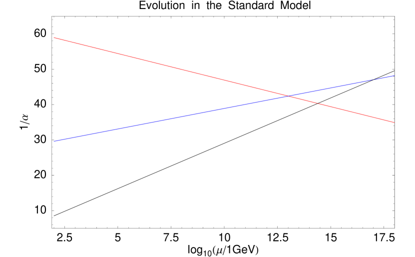
Figure 7: Values of the gauge couplings of the Standard Model at different scales. As input parameters we take $\alpha_{s}(M_{Z})_{\overline{MS}}=0.1187$, $\alpha(M_{Z})_{\overline{MS}}=1/127.906$, and $\sin^{2}\theta_{W}(M_{Z})_{\overline{MS}}=0.2312$. Here the three couplings do not have a common intersection.

Next we consider the minimal non-supersymmetric $SU(5)$, where the matter is unified in ${\bar{5}}$ and ${10}$, the Higgs sector is composed by ${5_{H}}=(H,T)$ and ${24_{H}}=(\Sigma_{8},\Sigma_{3},\Sigma_{(3,2)},\Sigma_{(\bar{3},2)},\Sigma_{24})$, while the gauge fields live in ${24_{V}}$. Using the SM decomposition one gets the following equations for the $B_{i}$,

$$B_{1}^{SU(5)} = b_{1}^{SM}\ -\ \frac{105}{6}r_{V}\ +\ \frac{1}{15}r_{T}$$ (177)

$$B_{2}^{SU(5)} = b_{2}^{SM}\ +\ \frac{1}{3}r_{\Sigma_{3}}\ -\ \frac{21}{2}r_{V}$$ (178)

$$B_{3}^{SU(5)} = b_{3}^{SM}\ +\ \frac{1}{2}r_{\Sigma_{8}}\ -\ 7\ r_{V}\ +\ \frac{1}{6}r_{T}$$ (179)

where:

$$r_{I}=\frac{\ln M_{GUT}/M_{I}}{\ln M_{GUT}/M_{Z}}$$ (180)

and where $M_{I}$ is the mass of the additional particle $I$ ($M_{Z}\leq M_{I}\leq M_{GUT}$). Now, following Giveon et al [210], The equations for the running of the gauge couplings (replacing $b_{i}$ by $B_{i}$) can be put in a more suitable form in terms of differences in the coefficients $B_{ij}(=B_{i}-B_{j})$ and low energy observables [210]. One finds two relations that hold at $M_{Z}$ [210]

$$\frac{B_{23}}{B_{12}} = \frac{5}{8}\frac{\sin^{2}\theta_{w}-\alpha_{em}/\alpha_{s}}{3/8-\sin^{2}\theta_{w}},$$ (181)

$$\ln\frac{M_{GUT}}{M_{Z}} = \frac{16\pi}{5\alpha_{em}}\frac{3/8-\sin^{2}\theta_{w}}{B_{12}}.$$ (182)

Using the experimental values at $M_{Z}$ in the $\overline{MS}$ scheme [27] of $\sin^{2}\theta_{w}=0.23120\pm 0.00015$, $\alpha_{em}^{-1}=127.906\pm 0.019$ and $\alpha_{s}=0.1187\pm 0.002$, one obtains

$$\frac{B_{23}}{B_{12}} = 0.719\pm 0.005,$$ (183)

$$\ln\frac{M_{GUT}}{M_{Z}} = \frac{184.9\pm 0.2}{B_{12}}.$$ (184)

The above two relations constrain the mass spectrum of the extra particles that leads to an exact unification at $M_{GUT}$ and this approach offers a simple way to test unification for a given model. The fact that the SM with one Higgs doublet cannot yield unification is now more transparent in light of Eq.( 183). Namely, the resulting SM ratio is simply too small ($B_{23}^{SM}/B_{12}^{SM}=0.53$) to satisfy equality in Eq. (183). In minimal non-supersymmetric $SU(5)$ we have the same problem, since the colored triplet and superheavy gauge bosons have to be very heavy to avoid problem with proton decay $(B_{23}^{SU(5)}/B_{12}^{SU(5)}\leq 0.60)$. Now, in a minimal realistic non-supersymmetric grand unified theory based on $SU(5)$ [211], the Higgs sector is extended by ${15_{H}}=(\Phi_{a},\Phi_{b},\Phi_{c})$, where the fields $\Phi_{a}$, $\Phi_{b}$, and $\Phi_{c}$ transform as $(1,3,1)$, $(3,2,1/6)$ and $(6,1,-2/3)$, respectively. Here it is possible to generate neutrino masses, satisfy all experimental bounds on proton lifetimes and achieve unification. In this case we have additional contributions to the parameters $B_{12}$ and $B_{23}$ (see Table 3):

	Minimal $SU(5)$	$\Phi_{a}$	$\Phi_{b}$	$\Phi_{c}$
$B_{23}$	$B_{23}^{SU(5)}$	$\frac{2}{3}r_{\Phi_{a}}$	$\frac{1}{6}r_{\Phi_{b}}$	$-\frac{5}{6}r_{\Phi_{c}}$
$B_{12}$	$B_{12}^{SU(5)}$	$-\frac{1}{15}r_{\Phi_{a}}$	$-\frac{7}{15}r_{\Phi_{b}}$	$\frac{8}{15}r_{\Phi_{c}}$

Table 3: Contributions to the $B_{ij}$ coefficients in a realistic minimal non-SUSY $SU(5)$ [211].

A knowledge of $B_{12}$ and $B_{23}$ allows one to exhibit the entire parameter space where it is possible to achieve exact unification (See figure 8).

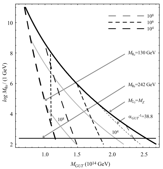
Figure 8: Plot of lines of constant $M_{\Sigma_{3}}$ and $M_{\Phi_{a}}$ in the $M_{GUT}$–$\textit{log}\,(M_{\Phi_{b}}/1\,\textrm{GeV})$ plane, assuming exact one-loop unification. The central values for the gauge couplings as given in the text are used. All the masses are given in GeV units. The triangular region is bounded from the left (below) by the experimental limit on $M_{\Phi_{a}}$ ($M_{\Phi_{b}}$). The right bound is $M_{\Sigma_{3}}\geq M_{Z}$. The two grey solid (thick dashed) lines are the lines of constant $M_{\Sigma_{3}}$ ($M_{\Phi_{a}}$). The line of constant $\alpha^{-1}_{GUT}\,$ is also shown. The region to the left of the vertical dashed line is excluded by the proton decay experiments if $\alpha=0.015$ GeV³ [212].

The triangular region in Fig. 8 represents the available parameter space under the assumption that $\Psi_{T}$, $\Sigma_{8}$ and $\Phi_{c}$ reside at or above the GUT scale. The region is bounded from the left and below by experimental limits on $M_{\Phi_{a}}$ and $M_{\Phi_{b}}$. The right bound stems from a requirement that $M_{\Sigma_{3}}\geq M_{Z}$. We note that in this scenario it is possible to predict the maximal value for the GUT scale, which allows one to define the upper bound on the proton decay lifetime (See Section 5.6 for details.). In this minimal non-supersymmetric scenario light leptoquarks $\Phi_{b}$ are predicted in order to achieve unification. Therefore it is a possibility to test the idea of grand unification at the next generation of collider experiments [211]. For studies in a different extension of the Georgi Glashow model see Ref. [213].

Let us investigate the constraints in supersymmetric scenarios. In the minimal supersymmetric standard model the equations for the running are given by:

$$B_{1}^{MSSM} = b_{1}^{SM}\ +\ \frac{21}{10}\ r_{\tilde{q}}\ +\ \frac{2}{5}\ r_{\tilde{G}}$$ (185)

$$B_{2}^{MSSM} = b_{2}^{SM}\ +\ 2\ r_{\tilde{G}}\ +\ \frac{13}{6}\ r_{\tilde{q}}$$ (186)

$$B_{3}^{MSSM} = b_{3}^{SM}\ +\ 2\ r_{\tilde{q}}\ +\ 2\ r_{\tilde{G}}$$ (187)

assuming the same mass $M_{\tilde{q}}$ for all scalars and the same mass for Higgsinos and gauginos $M_{\tilde{G}}$. In this case as is well-known it is possible to get unification at the scale $M_{GUT}\approx 10^{16}$ GeV, if the supersymmetric particles are around 1 TeV, or if one has only the gauginos and higgsinos at the $10^{2}$-$10^{3}$ GeV scale [214, 215, 216]. See Figure. (9) where we show the values of the gauge couplings at different scales in the context of the MSSM.

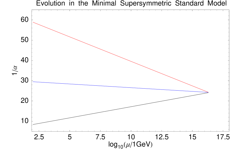
Figure 9: Values of the gauge couplings at different scales, in the $\overline{DR}$ scheme, in the context of the minimal supersymmetric standard model. For simplicity all superpartner masses are taken at $M_{Z}$ scale. The input parameters in the $\overline{MS}$ scheme are listed in Figure. (7). Here the gauge couplings unify at a high scale of $M_{G}\sim 2\times 10^{16}$ GeV.

To discuss the constraint on the Higgs triplet mass we list the equations for the running in the case of the minimal supersymmetric $SU(5)$:

$$B_{1}^{SSU(5)} = B_{1}^{MSSM}\ +\ \frac{2}{5}\ r_{T}\ -\ 10\ r_{V}$$ (188)

$$B_{2}^{SSU(5)} = B_{2}^{MSSM}\ +\ 2\ r_{\Sigma_{3}}\ -\ 6\ r_{V}$$ (189)

$$B_{3}^{SSU(5)} = B_{3}^{MSSM}\ +\ r_{T}\ -\ 4r_{V}\ +\ 3\ r_{\Sigma_{8}}$$ (190)

Assuming that $\Sigma_{3}$ and $\Sigma_{8}$ have the same mass and using the equations above one finds [217]:

$$(3\alpha_{2}^{-1}\ -\ 2\alpha_{3}^{-1}-\alpha_{1}^{-1})(M_{Z})=\frac{1}{2\pi}\ \left(\frac{12}{5}\ \ln\frac{M_{T}}{M_{Z}}-2\ \ln\frac{M_{SUSY}}{M_{Z}}\right)$$ (191)

Eq.(191) is a very useful in constraining the Higgs triplet mass. In reference [155] the authors concluded that the triplet mass $M_{T}\leq 3.6\times 10^{15}$ GeV, in order to satisfy the above constraint in the context of the minimal supersymmetric SU(5). However, when the fields $\Sigma_{3}$ and $\Sigma_{8}$ have different masses [159] the bound on $M_{T}$ is quite different. This is a possible solution, which implies that in the context of the minimal supersymmetric SU(5) it is still possible to satisfy the experimental bounds on proton decay lifetimes.

5.4 Testing GUTs through proton decay

As shown in the previous section the proton decay predictions arising from the gauge $d=6$ operators depend on the fermion mixing, i.e. the predictions are different in each model for fermion masses [43]. Let us analyze the possibility to test the realistic grand unified models, the $SU(5)$, the flipped $SU(5)$ and $SO(10)$ theories, respectively. Let us make an analysis of the operators in each theory, and study the physical parameters entering in the predictions for proton decay. Here we do not assume any particular model for fermion masses, in order to be sure that we can test the grand unification idea.

As an example we discuss now the specific case of $SU(5)$ with symmetric up Yukawa couplings. Here we consider the simplest grand unified theories, which are theories based on the gauge group $SU(5)$. In these theories the unification of quark and leptons is realized in two irreducible representations, $10$ and $\overline{5}$. The minimal Higgs sector is composed of the adjoint representation $\Sigma$, and two Higgses $5_{H}$ and $\overline{5}_{H}$ in the fundamental and anti-fundamental representations [9, 11]. If one wants to keep the minimal Higgs sector and have a realistic $SU(5)$ theory, one needs to introduce non-renormalizable operators, Planck suppressed operators, to get the correct quark-lepton mass relations. A second possibility is introduce a Higgs in the $45_{H}$ representation. In order to generate neutrino mass in these theories we have to add $15_{H}$ Higgs  (See for example [211]) or the right handed neutrinos. In this case we have only the operators $\textit{O}^{B-L}_{I}$ (Eq. 12), and $\textit{O}^{B-L}_{II}$ (Eq. 13) contributing to the decay of the proton. Let us study the prediction for proton decay in a $SU(5)$ theory with $Y_{U}=Y_{U}^{T}$. In this case we have $U_{C}=UK_{u}$, where $K_{u}$ is a diagonal matrix containing three phases which gives  [47]:

$$\sum_{l=1}^{3}c(\nu_{l},d_{\alpha},d^{C}_{\beta})_{SU(5)}^{*}c(\nu_{l},d_{\gamma},d^{C}_{\delta})_{SU(5)} = k_{1}^{4}(V_{CKM}^{*})^{1\alpha}(K_{2}^{*})^{\alpha\alpha}(V_{CKM})^{1\gamma}K_{2}^{\gamma\gamma}\delta^{\beta\delta}$$

In this case the clean channels to test the scenario are [47]:

$$\Gamma(p\to K^{+}\bar{\nu}) = k_{1}^{4}\left[A^{2}_{1}|V_{CKM}^{11}|^{2}+A^{2}_{2}|V_{CKM}^{12}|^{2}\right]C_{1}$$ (193)

$$\Gamma(p\rightarrow\pi^{+}\bar{\nu}) = k_{1}^{4}\left|V_{CKM}^{11}\right|^{2}C_{2}$$ (194)

where

$$C_{1} = \frac{(m_{p}^{2}-m_{K}^{2})^{2}}{8\pi m_{p}^{3}f_{\pi}^{2}}A_{L}^{2}\left|\alpha\right|^{2}$$ (195)

$$C_{2} = \frac{m_{p}}{8\pi f_{\pi}^{2}}A_{L}^{2}\left|\alpha\right|^{2}(1+D+F)^{2}$$ (196)

where the notation is as in Appendix G. Here we have two expressions for $k_{1}$, which are independent of the unknown mixing matrices and the phases. Thus it is possible to test $SU(5)$ grand unified theory with symmetric up Yukawa matrices through these two processes  [47]. These results are valid for any unified model based on $SU(5)$ with $Y_{U}=Y_{U}^{T}$. Similar tests can be investigated for other gauge groups. Specifically a discussion of the tests for the gauge groups $SO(10)$ and flipped $SU(5)$ is given in Appendix G.

5.5 Proton decay in flipped $SU(5)$

In the previous section we have shown the possibility to make a clear test of realistic grand unified theories with symmetric Yukawa couplings through the proton decay into a meson and antineutrinos. It is thus interesting to investigate how these conclusions change if one departs from the flavor structure of the minimal renormalizable theories. It is well known that the gauge $d=6$ proton decay cannot be rotated away, i.e., set to zero via particular choice of parameters entering in a grand unified theory, in the framework of conventional $SU(5)$ theory with the Standard Model particle content [218, 219]. So, it would appear that the gauge $d=6$ operators and proton decay induced by them are genuine features of matter unification. Now this conclusion has some caveats as we now discuss. To understand the issues more clearly it is useful to investigate the constraints that might allow one to rotate away the baryon and lepton number violating dimension six operators induced by gauge interactions. Thus consider the model based on conventional $SU(5)$. Setting $k_{2}=0$ in Eqs. (9)-(10) the relevant coefficients that enter in the decay rate formulas are:

$$c(e^{C}_{\alpha},d_{\beta})_{SU(5)} = k_{1}^{2}\left[V^{11}_{1}V^{\alpha\beta}_{2}+(V_{1}V_{UD})^{1\beta}(V_{2}V^{\dagger}_{UD})^{\alpha 1}\right]$$ (197)

$$c(e_{\alpha},d_{\beta}^{C})_{SU(5)} = k_{1}^{2}V^{11}_{1}V^{\beta\alpha}_{3}$$ (198)

$$c(\nu_{l},d_{\alpha},d^{C}_{\beta})_{SU(5)} = k_{1}^{2}(V_{1}V_{UD})^{1\alpha}(V_{3}V_{EN})^{\beta l},\ \textrm{$\alpha=1$ or $\beta=1$}$$ (199)

$$c(\nu_{l}^{C},d_{\alpha},d^{C}_{\beta})_{SU(5)} = 0$$ (200)

It is now easy to see that the demand to rotate away proton decay leads to conflict with experiment. In order to set Eq. (198) to zero, the only possible choice is $V_{1}^{11}=0$. [Setting $(V_{3})^{\beta\alpha}$ to zero would violate unitarity.] If we now look at Eq. (199), there is only one way to set to zero the coefficient entering in the decay channel into antineutrinos. Namely, we have to choose $(V_{1}V_{UD})^{1\alpha}=0$. This, however, is not possible since it would imply that, at least, $V_{CKM}^{13}$ is zero in conflict with experiment.

Next we investigate the same issue in flipped $SU(5)$. However, before doing so we give a brief discussion of it. The gauge group in this case is $SU(5)\times U(1)$ and the hypercharge is a linear combination of generators in $SU(5)$ and in $U(1)$, and so strictly speaking one does not have a unified gauge group. The particles reside in the multiplets $\bar{5}$, $10$ and in an SU(5) singlet and the assignments differ from those of the usual SU(5) as given in Appendix A. Thus in the flipped $SU(5)\times U(1)$ case the particle content of the multiplets is as below: For the $\bar{5}$ of SU(5) we have

$${\overline{5}}=\left(\begin{array}[]{c}u_{La}^{c}\\ e^{-}_{L}\\ -\nu_{eL}\end{array}\right)$$ (204)

where subscript a is the color index. For the 10 plet of $SU(5)$ and for the singlet we have

$$10=\left(\begin{array}[]{ccccc}0&d_{3}^{c}&-d_{2}^{c}&-u^{1}&-d^{1}\\ -d_{3}^{c}&0&d_{1}^{c}&-u^{2}&-d^{2}\\ d_{2}^{c}&-d_{1}^{c}&0&-u^{3}&-d^{3}\\ u^{1}&u^{2}&u^{3}&0&\nu^{C}\\ d^{1}&d^{2}&d^{3}&-\nu^{C}&0\end{array}\right)_{L},~{}~{}1=e^{+}$$ (210)

The $d=6$ proton decay from gauge interactions is again mediated by lepto quarks but their quantum number assignments are different so we label them with a prime: $V^{\prime}=(X^{\prime},Y^{\prime})$. This time the relevant $d=6$ coefficients are:

$$c(e^{C}_{\alpha},d_{\beta})_{SU(5)^{\prime}} = 0$$ (211)

$$c(e_{\alpha},d_{\beta}^{C})_{SU(5)^{\prime}} = k_{2}^{2}(V_{4}V^{\dagger}_{UD})^{\beta 1}(V_{1}V_{UD}V_{4}^{\dagger}V_{3})^{1\alpha}$$ (212)

$$c(\nu_{l},d_{\alpha},d^{C}_{\beta})_{SU(5)^{\prime}} = k_{2}^{2}V_{4}^{\beta\alpha}(V_{1}V_{UD}V^{\dagger}_{4}V_{3}V_{EN})^{1l},\ \textrm{$\alpha=1$ or $\beta=1$}$$ (213)

$$c(\nu_{l}^{C},d_{\alpha},d^{C}_{\beta})_{SU(5)^{\prime}} = k_{2}^{2}\left[(V_{4}V^{\dagger}_{UD})^{\beta 1}(U^{\dagger}_{EN}V_{2})^{l\alpha}+V^{\beta\alpha}_{4}(U^{\dagger}_{EN}V_{2}V^{\dagger}_{UD})^{l1}\right],$$

$$\alpha=1 \beta=1$$ or (214)

where the subscripts $SU(5)^{\prime}$ stands for flipped $SU(5)$. Let us see if it is possible to rotate away the proton decay in flipped $SU(5)$. To set Eq. (213) to zero, we can only choose $V_{4}^{\beta\alpha}=(D_{C}^{\dagger}D)^{\beta\alpha}=0$, where $\alpha=1$ or $\beta=1$. We could think about the possibility of making both Eqs. (212) and (5.5) zero, choosing $(V_{4}V_{UD}^{\dagger})^{\beta 1}=0$, however, this is in contradiction with the measurements of the CKM angles. Since in flipped $SU(5)$ the neutrino is Majorana, we only have to suppress Eq. (212). This can be accomplished by setting $(V_{1}V_{UD}V_{4}^{\dagger}V_{3})^{1\alpha}=(U_{C}^{\dagger}E)^{1\alpha}=0$ [220]. We note that this constraint is unrelated to the constraint on $V_{4}$. Thus, there is no contradiction with the unitarity constrains nor conflict with any experimental measurements of mixing angles. Consequently in the context of flipped $SU(5)$, it is possible to completely eliminate or rotate away the gauge $d=6$ contributions in a consistent way, by imposing the necessary conditions at 1 GeV [220].

In contrast in the minimal renormalizable flipped $SU(5)$ it is not possible to satisfy the first condition, since $Y_{D}=Y_{D}^{T}$ implies $V_{4}=K^{*}_{d}$, where $K_{d}$ is a diagonal matrix containing three phases. However, as discussed already we have to take into account the nonrenormalizable operators, which are important for fermion masses and which invariably lead to modification of naive predictions. Thus in general, in the context of flipped $SU(5)$, one is allowed to impose the necessary constraints and remove the gauge operators for proton decay. In summary the main difference between $SU(5)$ and flipped $SU(5)$ is that the unitary constraint that prevents one to eliminate proton decay in conventional $SU(5)$ does not operate in the latter case. In other words, the coefficients which depend on $\alpha$ and $\beta$ with $\alpha=1$ or $\beta=1$ have different consequences in those two scenarios [see Eqs. (198) and (213)].

5.6 Upper bound on the proton lifetime in GUTs

In the previous section we have discussed the different ways to test grand unified theories through the decay of the proton. In this section we discuss the possibility of finding an upper bound on the total proton decay lifetime [221]. In order to establish an upper bound on the total proton lifetime one may focus on the gauge $d=6$ contributions since all other contributions can be set to zero in searching for upper limits. Proton lifetime induced by superheavy gauge boson exchange can be written as follows

$$\tau_{p}=C\ M_{X}^{4}\ {\alpha^{-2}_{GUT}}\ m_{p}^{-5}$$ (215)

Here $C$ is a coefficient which contains all information about the flavor structure of the theory, $M_{X}$ is the mass of the superheavy gauge bosons, and $\alpha_{GUT}=g^{2}_{GUT}/4\pi$, where $g_{GUT}$ is the coupling defined at the GUT scale (the scale of gauge unification). To find a true upper bound on the total lifetime the maximal value of $C$ is needed. Then, for a given value of $M_{X}$ and $\alpha_{GUT}$ it is possible to bound the GUT scenario prediction for the nucleon lifetime. However, minimization of the total decay rate is very difficult since in principle 42 unknown parameters enter in the decay. The upper bound on the proton lifetime in the case of Majorana neutrinos reads as:

$$\tau_{p}\leq 6.0^{+0.5}_{-0.3}\times 10^{39}\ \frac{(M_{X}/10^{16}\,\textrm{GeV})^{4}}{\alpha_{GUT}^{2}}\ (0.003\,\textrm{GeV}^{3}/\alpha)^{2}\,\textrm{years}$$ (216)

where the gauge boson mass is given in units of $10^{16}$ GeV. Details of the analysis is given in Appendix H and here we present only the results [221].

The proton decay bounds in the $M_{X}$–$\alpha_{GUT}$ plane for the Majorana (Dirac) neutrino case are in Fig. 10 (11). These results, in conjunction with the experimental limits on nucleon lifetime, set an absolute lower bound on mass of superheavy gauge bosons. Since their mass is identified with the unification scale after the threshold corrections are incorporated in the running this also sets the lower bound on the unification scale. Using the most stringent limit on partial proton lifetime ($\tau_{p}\geq 50\times 10^{32}$ years) for the $p\rightarrow\pi^{0}e^{+}$ channel [27] and setting $\alpha=0.003$ GeV³, the bound on $M_{X}$ reads:

$$M_{X}\geq 3.04^{+0.3}_{-0.3}\times 10^{14}\sqrt{\alpha_{GUT}}\,\textrm{GeV}$$ (217)

where $\alpha_{GUT}$ usually varies from $1/40$ for non-supersymmetric theories to $1/24$ for supersymmetric theories. For example, if we take a non-supersymmetric value $\alpha_{GUT}=1/39$, one obtains

$$M_{X}\geq 4.9\times 10^{13}\,\textrm{GeV}$$ (218)

We note that the above result implies that any non-supersymmetric theory with $\alpha_{GUT}=1/39$ is eliminated if its unifying scale is bellow $4.9\times 10^{13}$ GeV regardless of the exact form of the Yukawa sector of the theory. Further, a majority of non-supersymmetric extensions of the Georgi-Glashow $SU(5)$ model yield a GUT scale which is slightly above $10^{14}$ GeV. Hence, as far as the experimental limits on proton decay are concerned, these extensions still represent viable scenarios of models beyond the SM. Region of $M_{X}$ excluded by the experimental result is also shown in Figs. 10 and 11. The plots of Fig.(10,11) exhibit that it is possible to satisfy all experimental bounds on proton decay in the context of non-supersymmetric grand unified theories. For example in a minimal non-supersymmetric GUT [211] based on $SU(5)$ the upper bound on the total proton decay lifetime is $\tau_{p}\ \leq\ 1.4\times 10^{36}$ years [212].

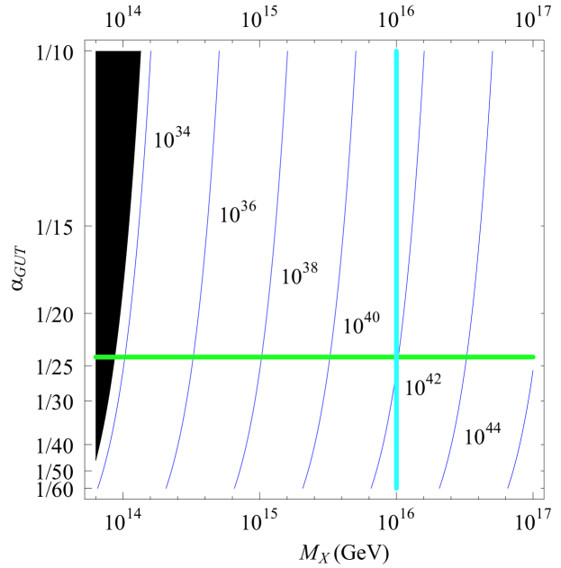
Figure 10: Isoplot for the upper bounds on the total proton lifetime in years in the Majorana neutrino case in the $M_{X}$–$\alpha_{GUT}$ plane. The value of the unifying coupling constant is varied from $1/60$ to $1/10$. The conventional values for $M_{X}$ and $\alpha_{GUT}$ in SUSY GUTs are marked in thick lines. The experimentally excluded region is given in black [221]

.

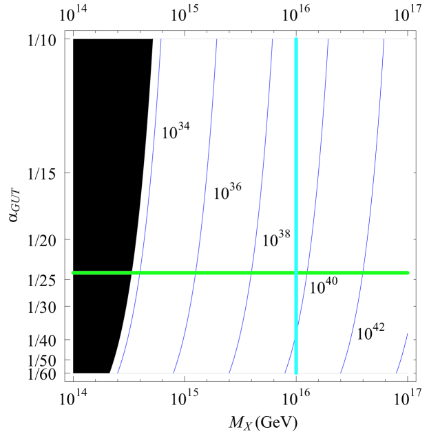
Figure 11: Isoplot for the upper bounds on the total proton lifetime in years in the Dirac neutrino case in the $M_{X}$–$\alpha_{GUT}$ plane. The value of the unifying coupling constant is varied from $1/60$ to $1/10$. The conventional values for $M_{X}$ and $\alpha_{GUT}$ in SUSY GUTs are marked in thick lines. The experimentally excluded region is given in black [221]

.

6 Unification in Extra Dimensions and Proton Decay

Over the recent past models based on large extra dimensions have received considerable attention. The largeness of the extra dimension implies that the compactification scale is small compared to the Planck scale, and guided by a desire for new physics at accelerators this scale is often chosen to lie in the TeV region, limited only by the constraints of the precision data. The extreme smallness of the compactification scale compared to the GUT scale or Planck scale implies that baryon and lepton number violating dimension six operators would only be suppressed by the inverse of the TeV scale and thus lead to unacceptable rate for proton decay. This is an important hurdle for the large extra dimension models. In this section we discuss various scenarios where proton stability can be achieved in such models with the help of discrete symmetries. We briefly outline the main items discussed in this section.

In Sec.(6.1) we consider grand unified models based on one extra space-time dimension, and discuss proton stability within such models. It is shown that with discrete symmetries it is possible to get a natural doublet-triplet splitting in the Higgs sector. In Sec.(6.2) we give a review of SO(10) models based in 5D, and give a discussion of 5D trinification models in Sec.(6.3). Sec.(6.4) is devoted to a discussion of grand unification models in 6D, where several unification scenarios are analyzed. These include $SO(10)$, $SU(5)\times U(1)$, flipped $SU(5)\times U(1)$, and $SU(4)_{C}\times SU(2)_{L}\times SU(2)_{R}$. In Sec.(6.5) we discuss gauge-Higgs unification. Here the Higgs fields arise as part of the gauge multiplet and thus gauge and Higgs couplings are unified. In these models proton decay is sensitive to how matter is located in extra dimensions. A discussion of proton decay in models with universal extra dimensions (UED) is given in Sec.(6.6). Proton decay is suppressed in these models due to the existence of extra symmetries. In Sec.(6.7) we give a discussion of proton stability in models with warped geometry. In this class of models proton stability arises via a symmetry which conserves the baryon number. Sec.(6.8) is devoted to a discussion of proton stability in kink backgrounds.

6.1 Proton decay in models with 5D

In this subsection we discuss proton decay in theories with one extra dimension. Theories with extra dimensions have a long history beginning with the work of Kaluza and Klein in the nineteen twenties [222, 223, 224, 225]. More recently interest in theories with extra dimensions emerged with the realization that string theories could allow for low scale compactifications which removes the rigid relationship that exists between the string scale and the Planck scale in the weakly coupled heterotic strings [226]. Thus, in the context of the weakly coupled Type I string compactifications the string scale can be quite low [227, 228] and there has been much work in model building along these lines [229, 230, 231, 232] and important constraints have been placed on the size of such dimensions from experiment [233, 234, 235]. An interesting phenomena in such theories is the power law evolution of the gauge coupling constants [236, 237, 238, 239] which allows for a meeting of the coupling constants at a low scale although in such a scheme the unification of the gauge couplings is not a prediction of the model but rather an accident. The second more serious issue concerns stability of the proton. This is so because if one wishes to formulate unified models with low scale extra dimensions then dimension five and dimension six baryon and lepton number violating operators are suppressed only by the inverse powers of a mass order a TeV which would lead to disastrous proton decay. An early suggestion to achieve proton stability is to have quarks - leptons in the bulk [240]. In the model of Ref. [240] $B$ and $L$ are separately conserved and the proton is stable with a unification scale in the TeV region. In this model TeV scale mirror particles could be produced at colliders [240]. Another way to suppress proton decay is to assume that the baryon number is gauged in the bulk and the symmetry is broken on a brane different from the physical brane [241]. Other suggestions to suppress proton decay require imposition of discrete symmetries [237, 232, 242, 243]. Such discrete symmetries are discussed in detail in Ref. [242] where a generalized matter parity of the type $Z_{3}\times Z_{3}$ is proposed in an extended MSSM type model where proton decay operators are suppressed to high orders. However, suppression of proton decay may require an exact or almost exact baryon number conservation, since otherwise proton decay may be induced by quantum gravity effects [244]. It is argued that in order to suppress this type of proton decay one would need a high scale similar to what one has in grand unified theories [244].

We would not pursue further the analysis of proton decay in extra dimension theories with low scale. Rather, we turn our attention now to the more realistic scenarios with high scale extra dimensions. Typically this is the situation in heterotic string models where the size of the extra dimension is of order the inverse of the compactification scale $M_{C}$ which one expects is close to the string scale. It turns out that the study of such models do have important benefits, the most prominent being that they provide a natural solution to the doublet-triplet splitting in the Higgs sector. Often they also lead to a reduction of the gauge symmetries without the necessity of invoking the Higgs mechanism. Thus, we consider grand unified theories in higher dimensions where reduction to 4 dimensions is accomplished by orbifold compactification. It has been known for some time that an orbifold compactification can reduce symmetries beginning with the work of Scherk and Schwarz [245, 246] and follow up works [247, 248, 249, 250]. (For a discussion of generalized symmetry breaking on orbifolds see Refs. [251, 252]). Orbifold compactifications have played a major role in recent works in the exploration of low scale extra dimensions putting lower limits of a few TeV on such dimension [233, 234, 235]. More recently interest has focused on grand unified models with extra dimensions and here an interesting development is the reduction of the gauge symmetry by orbifold compactification [253, 254, 255, 256, 251, 257] which has in addition some very interesting features such as automatic doublet-triplet splitting. The simplest possibility is a GUT theory formulated in 5 dimensions. Thus let us consider a 5D space with coordinates $x^{M}=(x^{\mu},x^{5})$ where $\mu=0,1,2,3$. We assume that the fifth dimension $x^{5}$ is compacted on $S^{1}/(Z_{2}\times Z_{2}^{\prime})$ where the $Z_{2}$ and $Z_{2}^{\prime}$ are defined as follows: $Z_{2}$ corresponds to the transformation

$$x^{5}\to-x^{5}$$ (219)

while $Z_{2}^{\prime}$ corresponds to the transformation

$$x^{5^{\prime}}\to-x^{5^{\prime}}$$ (220)

where $x^{5^{\prime}}=x^{5}+\pi R/2$. We focus on the $Z_{2}$ orbifolding first and return to the $Z_{2}^{\prime}$ orbifolding later. We begin by considering a super Yang-Mills field in the bulk. The $N=1$ super Yang-Mills in 5D consists of the multiplet $(V^{M},\Sigma,\lambda^{i},f^{a})$, where $V^{M}$ is the vector field with M=0,1,2,3,5, $\Sigma$ is a real scalar field, $\lambda^{i}$ are simplectic Majorana spinors and $f^{a}$ (a=1,2,3) are a triplet of auxiliary real fields [$V_{M}$ is a Lie valued quantity so that $V_{M}=gV_{M}^{\alpha}T^{\alpha}$ where $tr(T^{\alpha}T^{\beta})=\frac{1}{2}\delta_{\alpha\beta}$, and $\lambda$ and $\Sigma$ are similarly defined.]. For specificity we consider first the unified gauge group $SU(5)$ and assume that the super Yang Mills multiplet belongs to the adjoint representation of $SU(5)$. The 5D super Yang-Mills Lagrangian is given by [258, 259, 260]

$${\cal L}_{5}^{g} = \frac{1}{g^{2}}\{-\frac{1}{2}tr(V_{MN})^{2}+tr(D_{M}\Sigma)^{2}+tr(\bar{\lambda}i\gamma^{M}D_{M}\lambda)-tr(\bar{\lambda}[\Sigma,\lambda])$$ (221)

$$+ tr(f^{a})^{2}\}$$

where $D_{M}\sigma=\partial_{M}\Sigma-i[V_{M},\Sigma]$. The action is invariant under the following supersymmetry transformations

$$\delta_{\xi}V^{M} = i\bar{\xi}^{i}\gamma^{M}\lambda^{i}$$

$$\delta_{\xi}\Sigma = i\bar{\xi}^{i}\lambda^{i}$$

$$\delta_{\xi}\lambda^{i} = (\sigma^{MN}V_{MN}-\gamma^{M}D_{M}\Sigma)\xi^{i}-(f^{a}\sigma^{a})^{ij}\xi^{j}$$

$$\delta_{\xi}f^{a} = \bar{\xi}^{i}(\sigma^{a})^{ij}\gamma^{M}D_{M}\lambda^{j}-i[\Sigma,\bar{\xi}^{i}(\sigma^{a})^{ij}\lambda^{j}],$$ (222)

where $\xi^{i}$ are the transformation parameters and $\sigma^{MN}=[\gamma^{M},\gamma^{N}]/4$. From the 4D view point, the 5D N=1 vector multiplet is an N=2, 4D multiplet. We would like to reduce this multiplet to an N=1 multiplet on the $x^{5}=0$ brane which we consider to be the physical brane. To achieve this we consider the $Z_{2}$ transformation which acts on the bulk fields so that

$$f(x^{\mu},y)\to f(x^{\mu},-x^{5})=Pf(x^{\mu},x^{5})$$ (223)

where $P=\pm 1$. We take the fields $V_{\mu}$, $\lambda_{L}^{1}$, $f^{3}$ to have even parity, and the fields $V_{5},\Sigma,\lambda_{L}^{2},f^{1,2}$ to have odd parity. Further, we assign to $\xi_{L}^{1}$ an even parity and to $\xi_{L}^{2}$ an odd parity. Now the fields with odd parity vanish on the $x^{5}=0$ boundary, and the transformations on the $x^{5}=0$ brane reduce to the following [261]

$$\delta_{\xi}V^{\mu}=i\bar{\xi}^{1\dagger}_{L}\bar{\sigma}^{\mu}\lambda_{L}^{1}-i\lambda^{1\dagger}_{L}\bar{\sigma}^{\mu}\xi^{1}_{L}$$

$$\delta_{\xi}\lambda_{L}^{\prime}=\sigma^{\mu\nu}V_{\mu\nu}\xi^{1}_{L}-iD\xi_{L}^{1}$$

$$\delta_{\xi}D=i\bar{\xi}^{1\dagger}_{L}\bar{\sigma}^{\mu}D_{\mu}\lambda_{L}^{1}+h.c.$$ (224)

where $D\equiv(f^{3}-\partial_{5}\Sigma)$. Eqs.(224) constitute the transformations of an N=1 gauge multiplet with components

$$V_{\mu},\lambda_{L}^{1},D\equiv(f^{3}-\partial_{5}\Sigma)$$ (225)

on the $x^{5}=0$ brane. We note the appearance of $\partial_{5}\Sigma$ in the auxiliary field D. While $\Sigma$ has odd $Z_{2}$ parity and vanishes on the $x^{5}=0$ brane, $\partial_{5}\Sigma$ has even $Z_{2}$ parity and is non-vanishing on the $x^{5}=0$ boundary.

Analogous to the vector multiplet we assume that the Higgs multiplets reside also in the bulk and for model building we consider two hypermultiplets consisting of two complex scalar fields and two Dirac fermions $(H_{i}^{s},\psi^{s})$ (i=1,2) where $H_{i}^{s}$ are complex Higgs doublets and $\psi^{s}$ are Dirac spinors. We identify these multiplets as follows

$$\{(H^{1}_{1},\psi_{R}^{1}),(H_{2}^{1},\psi_{L}^{1})\}$$

$$\{(H^{2}_{1},\psi_{R}^{2}),(H_{2}^{2},\psi_{L}^{2})\}$$ (226)

The 5D bulk Lagrangian for the Higgs multiplet is then given by [259]

$${\cal L}_{5}^{H}=|D_{M}H_{i}^{s}|^{2}+i\bar{\psi}_{s}\gamma^{M}D_{M}\psi^{s}-(i\sqrt{2}H_{s}^{i\dagger}\bar{\lambda}_{i}\psi^{s}+h.c.)$$

$$-\bar{\psi}_{s}\Sigma\psi^{s}-H_{s}^{i\dagger}(\Sigma)^{2}H_{i}^{s}-\frac{g^{2}}{2}\sum_{m.\alpha}[H_{s}^{i\dagger}(\sigma^{m})^{j}_{i}T^{\alpha}H_{j}^{s}]^{2}$$ (227)

However, care is needed in the reduction of the Higgs bulk Lagrangian to the boundary. Analogous to the case of the vector multiplet one should begin with off shell hypermultiplets $(H^{s}_{i},\psi^{s},F_{i}^{s})$ which break up into the $Z_{2}$ parity even multiplets $(H^{1}_{1},\psi_{R}^{1},F_{1}^{1})$, $(H_{2}^{2},\psi_{L}^{2},F_{2}^{2})$ and the $Z_{2}$ parity odd multiplets $(H_{2}^{1},\psi_{L}^{1},F_{2}^{1})$, $(H^{2}_{1},\psi_{R}^{2},F^{2}_{1})$. As we go to the boundary $x^{5}=0$ only the $Z_{2}$ even parity multiplets survive and the surviving multiplets are [258, 259] ${\cal H}_{1}=(H_{1}^{1\dagger},\bar{\psi}_{R}^{1},F_{1}^{\dagger})$, and ${\cal H}_{2}=(H_{2}^{2},\psi_{L}^{2},F_{2})$ where $F_{1}=F_{1}^{1}-\partial_{5}H_{2}^{1}$ and $F_{2}=F_{2}^{2}-\partial_{s}H_{1}^{2}$. Here ${\cal H}_{2}$ is the multiplet that couples to the up quark and ${\cal H}_{1}$ is the multiplet that couples to the down quark and the lepton. We note that on the boundary the auxiliary fields are modified and this phenomenon is much similar to the modification of the D term on the boundary discussed above for the case of the vector multiplet.

In the preceding analysis we have seen that the action of $Z_{2}$ orbifolding reduces N=2 supersymmetry down to $N=1$ supersymmetry on the boundary. However, the SU(5) gauge symmetry is left intact. We consider now the action of the $Z_{2}^{\prime}$ orbifolding which leaves the $N=1$ supersymmetry intact but reduces the $SU(5)$ gauge symmetry down to the Standard Model gauge group. To accomplish this we consider $Z_{2}^{\prime}$ transformation such that the field $f(x^{\mu},x^{5})$ which belongs to the fundamental representation of $SU(5)$ transforms so that

$$f(x^{\mu},x^{5^{\prime}})\to f(x^{\mu},-x^{5^{\prime}})=P^{\prime}f(x^{\mu},x^{5^{\prime}})$$ (228)

where $x^{5^{\prime}}=x^{5}+\pi R/2$ and $P^{\prime}$ is a $5\times 5$ matrix with $P^{\prime}=diag(-1,-1,-1,1,1)$. Thus the fields with $SU(3)_{C}$ color indices will transform with parity $-$ and the fields with $SU(2)$ indices will transform with $Z_{2}^{\prime}$ parity $+$. We identify $H_{5}$ with $H_{2}^{2}$ as the one that gives mass to the up quarks, and $H_{\bar{5}}$ with $H_{1}^{1}$ which gives mass to the down quarks and the leptons. Similarly, we define $\hat{H}_{\bar{5}}=H^{2}_{1}$ and $\hat{H}_{5}=H^{1}_{2}$. One has then the following transformations for the Higgs multiplets under $Z_{2}^{{}^{\prime}}$ transformations

$$H_{5}(x^{\mu},x^{5^{\prime}})\to H_{5}(x^{\mu},-x^{5^{\prime}})=P^{\prime}H_{5}(x^{\mu},x^{5^{\prime}}),$$

$$H_{\bar{5}}(x^{\mu},x^{5^{\prime}})\to H_{\bar{5}}(x^{\mu},-x^{5^{\prime}})=P^{\prime}H_{\bar{5}}(x^{\mu},x^{5^{\prime}}),$$

$$\hat{H}_{5}(x^{\mu},x^{5^{\prime}})\to\hat{H}_{5}(x^{\mu},-x^{5^{\prime}})=-P^{\prime}\hat{H}_{5}(x^{\mu},x^{5^{\prime}}),$$

$$\hat{H}_{\bar{5}}(x^{\mu},x^{5^{\prime}})\to\hat{H}_{\bar{5}}(x^{\mu},-x^{5^{\prime}})=-P^{\prime}\hat{H}_{\bar{5}}(x^{\mu},x^{5^{\prime}}).$$ (229)

Thus under $Z_{2}\times Z_{2}^{\prime}$ transformations a field can be classified as $f_{\pm\pm}(x^{\mu},x^{5})$. It is instructive to carry out a normal mode expansion for these.

$$f_{++}(x,x^{5}) = \sqrt{1\over{\pi R}}\sum_{n=0}^{\infty}\frac{1}{\sqrt{2^{\delta_{n,0}}}}f^{(2n)}_{++}(x)\cos({2nx^{5}\over R}),$$

$$f_{+-}(x,x^{5}) = \sqrt{1\over{\pi R}}\sum_{n=0}^{\infty}f^{(2n+1)}_{+-}(x)\cos({(2n+1)x^{5}\over R}),$$

$$f_{-+}(x,x^{5}) = \sqrt{1\over{\pi R}}\sum_{n=0}^{\infty}f^{(2n+1)}_{-+}(x)\sin({(2n+1)x^{5}\over R}),$$

$$f_{--}(x,x^{5}) = \sqrt{1\over{\pi R}}\sum_{n=0}^{\infty}f^{(2n+2)}_{--}(x)\sin({(2n+2)x^{5}\over R}).$$ (230)

The above implies that the modes $f^{(2n)}_{++},f^{(2n+1)}_{+-},f^{(2n+1)}_{-+},f^{(2n+2)}_{--}$ have masses $2n/R$, $(2n+1)/R$, $(2n+1)/R$ and $(2n+2)/R$. One notices that only $f_{++}$ contains massless modes corresponding to the case when $n=0$. The other modes all acquire masses scaled by the inverse of the compactification radius, i.e., proportional to $1/R$. We exhibit the mode expansion for the Higgs multiplets in Table (4) where we have decomposed the Higgs $5$ plets in SU(3) color triplets, and $SU(2)$ doublets and the Higgs $\bar{5}$ in the SU(3) color anti-triplets, and $SU(2)$ doublets, i.e., $H_{5}=(H_{u},H_{T})$, $H_{\bar{5}}=(H_{d},H_{\bar{T}})$, $\hat{H}_{5}=(\hat{H}_{u},\hat{H}_{T})$, and $\hat{H}_{\bar{5}}=(\hat{H}_{d},\hat{H}_{\bar{T}})$.

4D fields	$Z_{2}\times Z_{2}^{\prime}$ parity	Mass
$H^{(2n)}_{u}$	(+,+)	2n/R
$\hat{H}^{(2n)}_{u}$	$(-,-)$	(2n+2)/R
$H^{(2n)}_{d}$	$(+,+)$	2n/R
$\hat{H}^{(2n+2)}_{d}$	$(-,-)$	(2n+2)/R
$H_{T}^{(2n+1)}$	$(+,-)$	(2n+1)/R
$H_{\bar{T}}^{(2n+1)}$	$(+,-)$	(2n+1)/R
$\hat{H}_{T}^{(2n+1)}$	$(-,+)$	(2n+1)/R
$\hat{H}_{\bar{T}}^{(2n+1)}$	$(-,+)$	(2n+1)/R

Table 4: P and ${\rm P}^{\prime}$ parities of the components of bulk Higgs multiplets.

In Table (4) the entries above the double horizontal line are the Higgs doublet modes. Here for $n=0$ we have massless modes in $H_{u}$ and $H_{d}$. The entries below the double horizontal line are the Higgs triplets (denoted by the subscript $T$) and the color anti-triplets (denoted by the subscript $\bar{T}$). Here we see that none of the Higgs triplets and anti-triplets have massless modes. Thus we see a natural doublet-triplet splitting by the assignment of the parities as described above. The Higgs triplets and anti-triplet produce a tower of massive Kaluza-Klein modes whose masses are scaled by the inverse radius of the circle $S^{1}$.

We look now at the transformation properties of the vector multiplet. These fields have transformations like bi-fundamentals because they carry two $SU(5)$ indices. It is easily seen that the Lagrangian is invariant under the following $Z_{2}^{\prime}$ transformations

$$V_{\mu}(x^{\mu},x^{5^{\prime}})\to V_{\mu}(x^{\mu},-x^{5^{\prime}})=P^{\prime}V_{\mu}(x^{\mu},x^{5^{\prime}})P^{{}^{\prime}-1},$$ (231)

$$\lambda_{L}^{1}(x^{\mu},x^{5^{\prime}})\to\lambda_{L}^{1}(x^{\mu},-x^{5^{\prime}})=P^{\prime}\lambda_{L}^{1}(x^{\mu},x^{5^{\prime}})P^{{}^{\prime}-1},$$

$$\lambda_{L}^{2}(x^{\mu},x^{5^{\prime}})\to\lambda_{L}^{2}(x^{\mu},-x^{5^{\prime}})=-P^{\prime}\lambda_{L}^{2}(x^{\mu},x^{5^{\prime}})P^{{}^{\prime}-1},$$

$$\Sigma(x^{\mu},x^{5^{\prime}})\to\Sigma(x^{\mu},-x^{5^{\prime}})=-P^{\prime}\Sigma(x^{\mu},x^{5^{\prime}})P^{{}^{\prime}-1}$$

$$V_{5}(x^{\mu},x^{5^{\prime}})\to V_{5}(x^{\mu},-x^{5^{\prime}})=-P^{\prime}V_{5}(x^{\mu},x^{5^{\prime}})P^{{}^{\prime}-1}$$

It is easy to infer that the transformation of the generators of $SU(5)$ under $P^{\prime}$ are

$$P^{\prime}T^{a}P^{{}^{\prime}-1}=T^{a},~{}~{}P^{\prime}T^{\hat{a}}P^{{}^{\prime}-1}=-T^{\hat{a}}$$ (232)

where $T^{a}$ are the generators of the Standard Model gauge group $G_{\rm SM}$ and $T^{\hat{a}}$ are in the remaining set. The mode expansion of the vector multiplet components is listed in Table 5 where the subscripts $\pm$ on the modes specify their properties under $Z_{2}\times Z_{2}^{\prime}$ transformations. We find that only the fields with $(+,+)$ parities have zero modes and they transform under $SU(3)_{C}\times SU(2)_{L}$ as $(8,1)+(1,3)+(1,1)$. These zero modes are precisely the gauge vector multiplets of MSSM which we label $V_{\mu}^{a}$. All the remaining vector fields $V_{\mu}^{\hat{a}}$, i.e., the lepto-quarks, acquire masses. Specifically, we note that the vector multiplet which transforms like $(3,2)+(\bar{3},2)$ under $SU(3)_{C}\times SU(2)$ has only massive modes. Thus the above orbifolding naturally splits the lepto-quarks from the Standard Model gauge bosons.

4D fields	$SU(3)\times SU(2)$ reps	Mass
$V_{\mu++}^{a(2n)}$, $\lambda_{++}^{1a(2n)}$	$(8,1)+(1,3)+(1,1)$	2n/R
$V_{5--}^{a(2n+2)}$,$\lambda_{--}^{2a(2n+2)}$, $\Sigma_{--}^{a(2n+2)}$	$(8,1)+(1,3)+(1,1)$	(2n+2)/R
$V_{\mu+-}^{\hat{a}(2n+1)}$, $\lambda_{+-}^{1\hat{a}(2n+1)}$	$(3,2)+(\bar{3},2)$	(2n+1)/R
$V_{5-+}^{\hat{a}(2n+1)}$,$\lambda_{-+}^{2\hat{a}(2n+1)}$, $\Sigma_{-+}^{\hat{a}(2n+1)}$	$(3,2)+(\bar{3},2)$	(2n+1)/R

Table 5: P and ${\rm P}^{\prime}$ parities for the components of bulk gauge multiplets

In setting up the Lagrangian in 5D we have to make sure that the Lagrangian is invariant under the full $Z_{2}\times Z_{2}^{\prime}$ transformations. This set up is dependent on how the matter is located in the 5D space. One could locate such matter either in the bulk, or on the orbifolds. There are two invariant orbifold points corresponding to $x^{5}=0$ and $x^{5}=\pi R/2$ which are the end points of the fundamental domain $x^{5}=(0,\pi)$. When matter, is located at the $x^{5}=0$ brane, one can maintain the full $SU(5)$ symmetry, while when matter is located at the $x^{5}=\pi R/2$ brane, only the standard model symmetry can be maintained. In fact, there are three scenarios for the location of matter and we classify the three possibilities as follows [257, 262, 256].

1. Matter on the SU(5) brane

2. Matter in the bulk

3. Matter on the SM brane

Let us begin by discussing case (1). We need to assign parities to the quark and lepton fields. For $Z_{2}$ transformations, P is $+$ for color and $+$ for SU(2). For quarks and leptons, one way to determine the $P^{\prime}$ parities is to require that cubic SU(5) invariant interactions with matter-matter-Higgs transform with an over all sign when one uses the $P^{\prime}$ parities of Higgs as given in Table (4). This gives the following possibilities

$$10:~{}~{}P^{\prime}(Q,U^{C},E^{C})=\eta_{10}(+,-,-)$$

$$\bar{5}:~{}~{}~{}~{}P^{\prime}(D^{C},L)=\eta_{\bar{5}}(-,+)$$ (233)

where $\eta_{\bar{5},10}$ are overall signs of $\bar{5}$ and $10$ multiplets, i.e., $\eta_{\bar{5},10}=\pm 1$. With the above we have

$$P^{\prime}(10.10.5_{H})=-(10.10.5_{H})$$

$$P^{\prime}(10.\bar{5}.\bar{5}_{H})=-\eta_{5}\eta_{10}(10.\bar{5}.\bar{5}_{H})$$ (234)

Using Eq.(234) we can write a $Z_{2}\times Z_{2}^{\prime}$ invariant 5D Yukawa interaction in the form

$${\cal{L}}_{5}=\int d^{2}\theta\frac{1}{2}(\delta(x^{5})-\delta(x^{5}-\pi R))f_{5u}10.10.5_{H}$$

$$+\int d^{2}\theta\frac{1}{2}(\delta(x^{5})-\eta_{\bar{5}}\eta_{10}\delta(x^{5}-\pi R))f_{5u}10.\bar{5}.\bar{5}_{H}+h.c.$$ (235)

The $Z_{2}\times Z_{2}^{\prime}$ invariance of Eq.(235) is easily checked by using Eq.(234). On integration over the fifth coordinate one gets the following effective Higgs-quark-lepton interaction in 4D

$${\cal{L}}_{4}={\cal{L}}_{0}+{\cal{L}}_{KK}$$ (236)

$${\cal{L}}_{0}=\int d^{2}\theta(f_{1}QU^{c}H_{u}^{(0)}+f_{2}QD^{c}H_{d}^{(0)}+f_{2}LEH_{d}^{(0)})+h.c.$$ (237)

$${\cal{L}}_{KK} = \sum_{n=1}^{\infty}\sqrt{2}\int d^{2}\theta(f_{1}QU^{c}H_{u}^{(2n)}+f_{2}QD^{c}H_{d}^{(2n)}+f_{2}LEH_{d}^{(2n)})$$ (238)

$$+ \sum_{n=1}^{\infty}\sqrt{2}\int d^{2}\theta(f_{1}QQH_{T}^{(2n+1)}+f_{1}U^{C}E^{C}H_{T}^{(2n+1)}+f_{2}QLH_{\bar{T}}^{(2n+1)}$$

$$+ f_{2}QLH_{\bar{T}}^{(2n+1)})$$

where $f_{1}=f_{5u}/\sqrt{2\pi R}$, $f_{2}=f_{5d}/\sqrt{2\pi R}$. One finds that ${\cal{L}}_{0}$ which contains the zero Higgs modes is precisely what one has in the minimal SU(5) theory for the Higgs doublets. However, unlike the minimal SU(5) of 4D theory, here one has a natural Higgs doublet-triplet splitting and one has no zero Higgs triplet modes. The ${\cal{L}}_{KK}$ contains the Kaluza-Klein excitations of the Higgs doublets and the Higgs triplets and anti-triplets.

There is no dimension five proton decay in this theory since the Higgs triplet mass terms are of the form [257]

$$\sum_{n=0}^{\infty}R^{-1}\int d^{2}\theta(H_{T}^{(2n+1)}\hat{H}_{T}^{(2n+1)}+H_{T}^{(2n+1)}\hat{H}_{T}^{(2n+1)})+h.c.$$ (239)

Since $\hat{H}$ does not connect to the quarks and leptons there is no dimension five proton decay mediated by Higgs triplets in this model. Further, as shown in Ref. [257] the model has an overall $U(1)_{R}$ invariance which kills the proton decay via dimension four operators from the term $10.\bar{5}.\bar{5}$ where all multiplets are matter multiplets. We pause to contrast the situation here with that in 4D supersymmetric theories. As discussed in Sec.5, in 4D supersymmetric grand unified theories, even with R parity one typically has baryon and lepton number  violating dimension five operators which lead to proton decay, and because of that there exist overlapping constraints on the GUT scale from the current experimental limits on the proton lifetime and from the gauge coupling unification. This issue lead us to consider in detail the twin constraints of gauge coupling unification in 4D theories and proton stability in Sec.(5.3). In contrast in higher dimensional theories of the type discussed above, one does not have any dimension five induced proton decay. However, the gauge coupling unification constraint can still affect proton decay via dimension six operators. Specifically, here Kaluza-Klein tower of states can affect proton decay lifetimes. A detailed discussion of this topic is given at the end of Sec.(6.4). It needs to be pointed out that the analysis of gauge coupling unification in higher dimensional theories in by no means unique, but rather has a significant model dependence. However, in a class of models the situation is even improved [263] over the supersymmetric $SU(5)$ model in 4D. A more detailed discussion of this topic is outside the scope of this report, but the reader is refereed to a number of recent works for an update[239, 264, 265, 257, 263].

Although, there no proton decay from dimension four and five operators in models of the above type, there is, however, proton decay from dimension six operators induced by gauge interactions.

Assuming that all the three generations are located on the SU(5) brane, one has a dimension six operator in this case, leading to a proton decay width for the mode $p\rightarrow e^{+}\pi^{0}$ which is [266]

$$\Gamma(p\rightarrow e^{+}\pi^{0})=(\frac{\pi g_{4}}{4M_{C}})^{4}\frac{5\alpha^{2}A_{R}^{2}m_{p}}{4\pi f_{\pi}^{2}}(1+D+F)^{2}.$$ (240)

With $F=0.47$, $D=0.8$, $f_{\pi}=0.13$ GeV, $\alpha=0.01$(GeV)³, $g^{2}_{4}/(4\pi)=0.04$ , $A_{R}=2.5$ one finds

$$\tau(p\rightarrow e^{+}\pi^{0})\simeq 1.4\times 10^{34}(\frac{M_{C}}{10^{16}\rm{GeV}})^{4}\rm{yr}.$$ (241)

The current experiment already puts a lower limits on $M_{C}$ of $M_{C}\simeq 8\times 10^{15}$ GeV.

We consider now case (2) where one has matter in the bulk. Here one starts with complete SU(5) multiplets involving 10 and $\bar{5}$. However, $P^{\prime}$ splits these so that only certain components of these multiplets have zero modes. For example, with a specific choice of $P^{\prime}$ parities, only $U^{c}$ and $E^{c}$ in the 10 plet and only $D^{c}$ in the $\bar{5}$ plet have zero modes. To complete the multiplets one can add a copy of the 10 and $\bar{5}$ which have an overall opposite $P^{\prime}$ parity to the previous multiplets. Since in this case the zero modes arise from different multiplets there are no X and Y gauge interactions which can produce baryon and lepton number violating dimension six operators. There are, however, Kaluza-Klein excitations of the bulk matter fields and X and Y gauge bosons do connect the zero modes matter fields with their KK counterparts. But these lead to operators which are at least dimension eight and suppressed by $M_{C}^{4}$. Their contributions to proton decay is far too small to be relevant.

Next we consider case (3) where one has matter confined to the SM brane. Here the X and Y boson wave-functions vanish at the location of the SM brane and thus one has no couplings of these gauge bosons to the SM matter fields and consequently no baryon and lepton number violating dimension six operator. So there is no proton decay from the usual X and Y boson exchange. However, we now show that non-minimal couplings such as derivative couplings can lead to proton decay. One can write in general on the SM brane a non-minimal operator with one derivative as follows [266]

$${\cal L}_{5N}=\frac{\gamma_{ij}}{M_{P}}\delta(x^{5^{\prime}})\int d^{2}\theta d^{2}\bar{\theta}\psi^{c\dagger}_{i}(D_{5}e^{2V})\psi_{j}+h.c.$$ (242)

The effective baryon and lepton number violating dimension 6 operators can be obtained by an integration over the X and Y gauge bosons, and one has

$$O_{6}\simeq\delta\gamma_{ij}\gamma_{kl}\frac{g_{4}^{2}}{M_{C}M_{P}}\int d^{2}\theta d^{2}\bar{\theta}\sum_{\hat{a}}(\psi^{c\dagger}_{i}T^{\hat{a}}\psi_{j})(\psi^{c\dagger}_{k}T^{\hat{a}}\psi_{l})$$ (243)

In the above $\gamma_{ij}$ and $\delta$ are strong interaction parameters which are typically O(1). The proton lifetime resulting from above is

$$\tau(p\rightarrow e^{+}\pi^{0})=3.5\times 10^{34}(\delta\gamma_{11})^{-2}(\frac{M_{C}^{1/2}M_{P}^{1/2}}{10^{16}\rm{GeV}})^{4}\rm{years}$$ (244)

Clearly the result of Eq.(244) has a significant model dependence. If one assumes that $M_{P}$ is around the Planck scale, since such type couplings are expected to arise from Planck scale corrections, one has $M_{P}\simeq 10^{18}$ GeV. Then an $M_{C}$ around $10^{15}$ GeV or larger, will put this lifetime out of reach of the next generation of experiments unless a suppression is manufactured from the front factors $(\delta\gamma_{11})^{-2}$.

6.2 SO(10) models in 5D

The SO(10) models in 5D which have been investigated by a number of authors [267, 268]. Here the gauge multiplet $\cal{V}$ is 45 dimensional belonging to the adjoint representation of SO(10). In 4D language the 5D vector multiplet will consist of the N=1 vector multiplet $V$ and an N=1 chiral multiplet $\Sigma$. We take the Higgs multiplet to lie in the 10 plet representation of SO(10) so in 5D it is a 10 dimensional hypermultiplet ${\cal H}_{10}$. In 4D it would correspond to two N=1 chiral superfields $H_{10},\hat{H}_{10}$. Similar to the SU(5) case we have the following transformations under $Z_{2}$

$$H_{10}(x^{\mu},x^{5})\to H_{10}(x^{\mu},-x^{5})=PH_{10}(x^{\mu},x^{5})$$

$$\hat{H}_{10}(x^{\mu},x^{5})\to\hat{H}_{10}(x^{\mu},-x^{5})=-P^{T}\hat{H}_{10}(x^{\mu},x^{5})$$ (245)

with $P^{2}=I$ where $P$ is now a $10\times 10$ matrix. We choose $P$ so that $P=1_{5\times 5}\times 1_{2\times 2}$. We assume similar transformations under $Z_{2}^{\prime}$, with $x^{5^{\prime}}$ replacing $x^{5}$ and $P^{\prime}$ replacing $P$ and for $P^{\prime}$ we choose [267, 268]

$$P^{\prime}=diag(-1,-1,-1,1,1)\times(1,1).$$ (246)

As in the case of SU(5) the $Z_{2}$ orbifolding breaks the N=2 supersymmetry in 4D to an N=1 supersymmetry . The $Z_{2}^{\prime}$ orbifolding breaks the SO(10) gauge group to an $SO(6)\times SO(4)$ gauge group. Since $SO(6)\sim SU(4)$ and $SO(4)\sim SU(2)_{L}\times SU(2)_{R}$, we classify the fields according to their $SU(4)\times SU(2)_{L}\times SU(2)_{R}$ representations. Thus the 45 plet of vector fields which belong to the adjoint representation of SO(10) can be classified in the $SU(4)_{C}\times SU(2)_{L}\times SU(2)_{R}$ representations as follows: V(15,1,1), V(1,3,1), V(1,1,3), V(6,2,2) and an identical decomposition holds for the 45 plet of the chiral scalar superfield $\Sigma$. The Higgs multiplets H and $\hat{H}$ which belong to the 10 plet representation of SO(10) decompose as H(6,1,1), H(1,2,2), $\hat{H}(6,1,1)$, $\hat{H}(1,2,2)$. The $Z_{2}\times Z_{2}^{\prime}$ properties of these fields are exhibited in Table. (6). The 16-plet spinor representation of SO(10) can be decomposed under $SU(4)_{C}\times SU(2)_{L}\times SU(2)_{R}$ as $(4,2,1)+(\bar{4},1,2)$. The generalization of a $Z_{2}^{\prime}$ transformation on a spinor is [267] $P^{\prime}=e^{-\frac{3\pi}{2}(B-L)}$. Now under the $SU(4)_{C}$ decomposition $SU(4)_{C}\to SU(3)_{C}\times U(1)_{B-L}$, one finds $(4,2,1)\to 3_{1/3}+1_{-1}$ which leads to $P^{\prime}=-i$ for the $(4,2,1)$ multiplet. Thus 16-pet spinor has $Z_{2}^{\prime}$ parities given by $(4,2,1)_{-i}+(\bar{4},1,2)_{i}$.

$SU(4)\times SU(2)_{L}\times SU(2)_{R}$ N=1 multiplets	$Z_{2}\times Z_{2}^{\prime}$ parities
V(15,1,1), V(1,3,1), V(1,1,3), H(1,2,2)	$(+,+)$
V(6,2,2), H(6,1,1)	$(+,-)$
$\Sigma(6,2,2)$, $\hat{H}(6,1,1)$	$(-,+)$
$\Sigma(15,1,1),\Sigma(1,3,1),\Sigma(1,1,3)$, $\hat{H}(1,2,2)$	$(-,-)$

Table 6: P and ${\rm P}^{\prime}$ parities of SO(10) vector and chiral multiplets

As discussed earlier in the $Z_{2}\times Z_{2}^{\prime}$ compactification there are two in-equivalent orbifold points: $x^{5}=0$ and $x^{5}=\pi R/2$. At $x^{5}=0$, the wave-functions for all the gauge bosons are non-vanishing and one has an SO(10) invariance. On the other hand at $x^{5}=\pi R/2$, the $V(6,2,2)$ gauge bosons have their wave-functions vanishing, and the gauge symmetry is reduced to $SU(4)_{C}\times SU(2)_{L}\times SU(2)_{R}$ . Thus we can classify the models at the two orbifold points as

1. SO(10) brane model

2. G(4,2,2) brane model

Analogous to the SU(5) 5D model there is no proton decay in these models from dimension 4 or dimension 5 operators. For the case of SO(10) brane proton decay from dimension six operators can occur. However, this proton decay is proportional to $M_{C}^{-4}$ as seen in Eq.(241). An estimate of $M_{C}$ for the model of Ref. [268] gives a value too low to be compatible with the current lower bounds on the proton lifetime. We focus next on the $G(4,2,2)$ brane model. Here to reduce the gauge symmetry further and to reduce the rank of the gauge group one needs to invoke the Higgs mechanism. One possibility is to consider addition of $16+\overline{16}$ of Higgs multiplets. Now under $SU(4)_{C}\times SU(2)_{L}\times SU(2)_{R}$ the 16 plet decomposes so that $16=(4,2,1)+(\bar{4},1,2)$ and one gives VEV to $\chi^{c}+\bar{\chi}^{c}$ where $\chi^{c}=(\bar{4},1,2)$. A VEV formation for this combination then breaks the $SU(4)_{C}\times SU(2)_{L}\times SU(2)_{R}$ symmetry down to the symmetry of the standard model gauge group. Since the wave-function for the $V(6,2,2)$ gauge bosons vanishes on the $SU(4)_{C}\times SU(2)_{L}\times SU(2)_{R}$ brane, there is no proton decay of the usual sort from the mediation of X and Y gauge bosons. However, proton decay can occur from derivative terms on the $SU(4)_{C}\times SU(2)_{L}\times SU(2)_{R}$ brane as given in Eq.(244). Analysis of gauge coupling unification in Ref. [268] gives an estimate of $M_{C}\sim 2\times 10^{14}$ GeV and $M_{P}$ is identified with the unification scale in string models and taken to be $\sim 2\times 10^{17}$ GeV. In this case the analysis of Ref. [268] gives

$$\tau(p\rightarrow e^{+}\pi^{0})\sim 7\times 10^{33\pm 2}{\rm yr}$$ (247)

where the $\pm 2$ reflects the uncertainties due to $\delta,\gamma_{11},M_{C}$ and $M_{P}$.

Another possible class of $SO(10)$ models in 5D is based on embedding of a four-dimensional flipped $SU(5)$ model in a five-dimensional $SO(10)$ model [269]. This approach can preserve the best features of both the flipped $SU(5)$ and of $SO(10)$. Namely, the missing partner mechanism, which naturally achieves both doublet-triplet splitting and suppression of dimension 5 proton decay operators, can be realized as in flipped $SU(5)$, while the gauge couplings unify as in $SO(10)$ [270].

In this approach orbifold compactification leaves two inequivalent points. One has an $SO(10)$ invariance while the other has flipped $SU(5)$ invariance. To break the rest of the way to the Standard Model one can either use Higgs fields that originate from the bulk [269] or reside on the flipped $SU(5)$ brane [270]. In both cases the split between the doublets and the triplets is done through the four-dimensional flipped-$SU(5)$ missing partner mechanism. As before, there is no proton decay from dimension 4 or dimension 5 operators. On the other hand, the strength of dimension 6 gauge contributions depends on the exact location of matter fields. If they originate from the bulk then the dimension 6 operators are strongly suppressed; if they are situated on either the $SO(10)$ or the flipped $SU(5)$ brane some suppression in the Yukawa sector is needed to avoid experimental bounds since $M_{C}\sim 5.5\times 10^{14}$ GeV [270].

6.3 5D Trinification

5D trinification models have also been considered [271, 272]. The trinification is based on the gauge group $SU(3)_{C}\times SU(3)_{L}\times SU(3)_{R}\times Z_{3}$ where the discrete symmetry permutes the three labels C,L,R which gives a single gauge coupling constant g at the unification scale. The gauge fields for the system can be decomposed in representations of $SU(3)_{C}\times SU(3)_{L}\times SU(3)_{R}$ so that they fall into the sets

$$(8,1,1)+(1,8,1)+(1,1,8)$$ (248)

The $Z_{2}\times Z_{2}^{\prime}$ parities of the vector multiplet V are defined as in Eq.(231) where $P,P^{\prime}$ are given by $P=P_{C}+P_{L}+P_{R}$ and similarly for $P^{\prime}$. We make the following assignments

$$(P_{C};P_{L};P_{R})=(1,1,1;1,1,-1;1,1,-1)$$

$$(P_{C}^{\prime};P_{L}^{\prime};P_{R}^{\prime})=(1,1,1;1,1,-1;1,1,1)$$ (249)

With the above assignments one has

$$V(8,1,1)~{}=~{}\left(\begin{array}[]{cc|c}(+,+)&(+,+)&(+,+)\\ (+,+)&(+,+)&(+,+)\\ \hline\cr(+,+)&(+,+)&(+,+)\end{array}\right),\qquad$$ (253)

$$V(1,8,1)~{}=~{}\left(\begin{array}[]{cc|c}(+,+)&(+,+)&(-,-)\\ (+,+)&(+,+)&(-,-)\\ \hline\cr(-,-)&(-,-)&(+,+)\end{array}\right),\qquad$$ (257)

$$V(1,1,8)~{}=~{}\left(\begin{array}[]{cc|c}(+,+)&(+,+)&(-,+)\\ (+,+)&(+,+)&(-,+)\\ \hline\cr(-,+)&(-,+)&(+,+)\end{array}\right).\qquad$$ (261)

Now as usual in addition to the possibility of putting matter in the bulk one may put matter on the $x^{5}=0$ brane or on the $x^{5}=\pi R/2$ brane. Suppose we consider the last possibility. In this case the gauge bosons odd under $P^{\prime}$ vanish at $x^{5}=\pi R/2$ and the gauge symmetry is reduced to $SU(3)_{C}\times SU(2)_{L}\times U(1)_{L}\times SU(3)_{R}$. There are no dimension six operators to produce proton decay in these models. In the usual triunification models, proton decay can arise from the dimension five operators generated by the Higgs triplets in the 27 plet representations. Here, however, since at the orbifold point one already has a reduced symmetry, a further reduction of the gauge symmetry involves only small representations [271]. Consequently there are no dimension five operators arising from them and hence there is no proton decay from this sector either.

6.4 6D models

There are a number of works which have explored GUT model building in 6D [273, 274, 275, 276, 277]. In such models one begins with a space $R^{4}\times T^{2}$ where $T^{2}$ is a two torus and one orbifolds $T^{2}$ in a way similar to what we discussed in 5D. One model studied in detail in the context of proton decay is the specific compactification [274, 275] $T^{2}/(Z_{2}\times Z_{2}^{\prime}\times Z_{2}^{{}^{\prime\prime}})$. The Lagrangian density for the vector multiplet in this case is

$${\cal L}_{6}=\frac{1}{g^{2}}tr(-\frac{1}{2}V_{MN}V^{MN}+i\bar{\lambda}\Gamma^{M}D_{M}\lambda)$$ (262)

where $\Gamma^{M}$ satisfy the Clifford algebra in 6D. Defining $V_{M}=(V_{\mu},V_{\alpha})$, where $\mu=0,1,2,3$ as usual and $\alpha=5,6$ the transformation properties of $V_{M},\lambda_{1},\lambda_{2}$ under $Z_{2}\times Z_{2}^{\prime}\times Z_{2}^{{}^{\prime\prime}}$ are

$$PV_{\mu}(x^{\mu},-x^{5},-x^{6})P^{-1}=V_{\mu}(x^{\mu},x^{5},x^{6}),$$

$$PV_{\alpha}(x^{\mu},-x^{5},-x^{6})P^{-1}=-V_{\alpha}(x^{\mu},x^{5},x^{6}),$$

$$P\lambda_{1}(x^{\mu},-x^{5},-x^{6})P^{-1}=\lambda_{1}(x^{\mu},x^{5},x^{6}),$$

$$P\lambda_{2}(x^{\mu},-x^{5},-x^{6})P^{-1}=-\lambda_{2}(x^{\mu},x^{5},x^{6}),$$ (263)

and we choose $P=I$. Here $(V_{\mu},\lambda_{1})$ form an N=1 vector multiplet and $(V_{\alpha},\lambda_{2})$ form an N=1 chiral multiplet. The zero modes arise only from the vector multiplet. Next under $Z_{2}^{{}^{\prime}}$

$$P^{\prime}V_{\mu}(x^{\mu},-x^{5},-x^{6}+\pi R_{6}/2)P^{{}^{\prime}-1}=V_{\mu}(x^{\mu},x^{5},x^{6}+\pi R_{6}/2),$$

$$P^{\prime}V_{\alpha}(x^{\mu},-x^{5},-x^{6}+\pi R_{6}/2)P^{{}^{\prime}-1}=-V_{\alpha}(x^{\mu},x^{5},x^{6}+\pi R_{6}/2),$$ (264)

where for $P^{\prime}$ we choose

$$P^{\prime}=diag(1,1,1,1,1)\times\sigma_{2}.$$ (265)

Similarly for $Z_{2}^{{}^{\prime\prime}}$

$$P^{{}^{\prime\prime}}V_{\mu}(x^{\mu},-x^{5}+\pi R_{5}/2,-x^{6})P^{{}^{\prime\prime}-1}=V_{\mu}(x^{\mu},x^{5}+\pi R_{5}/2,x^{6}),$$

$$P^{{}^{\prime\prime}}V_{\alpha}(x^{\mu},-x^{5}+\pi R_{5}/2,-x^{6})P^{{}^{\prime\prime}-1}=-V_{\alpha}(x^{\mu},x^{5}+\pi R_{5}/2,x^{6}),$$ (266)

where for $P^{{}^{\prime\prime}}$ we choose

$$P^{{}^{\prime\prime}}=diag(-1,-1,-1,1,1)\times\sigma_{0}.$$ (267)

Now the mode expansion of a function on the torus depends on its parities and there are eight cases corresponding to the eight permutations $\pm\pm\pm$. These have the following mode expansions

$$f_{+++}(x^{\mu},x^{\alpha})=\sum_{m\geq 0}(\pi^{2}R_{5}R_{6})^{-\frac{1}{2}}\frac{1}{2^{{\delta_{m,0}},{\delta_{n,0}}}}f_{+++}^{(2m,2n)}(x^{\mu})\cos(\frac{2mx^{5}}{R_{5}}+\frac{2nx^{6}}{R_{6}})$$

$$f_{++-}(x^{\mu},x^{\alpha})=\sum_{m\geq 0}(\pi^{2}R_{5}R_{6})^{-\frac{1}{2}}f_{++-}^{(2m,2n+1)}(x^{\mu})\cos(\frac{2mx^{5}}{R_{5}}+\frac{(2n+1)x^{6}}{R_{6}})$$

$$f_{+-+}(x^{\mu},x^{\alpha})=\sum_{m\geq 0}(\pi^{2}R_{5}R_{6})^{-\frac{1}{2}}f_{+-+}^{(2m+1,2n)}(x^{\mu})\cos(\frac{(2m+1)x^{5}}{R_{5}}+\frac{2nx^{6}}{R_{6}})$$

$$f_{+--}(x^{\mu},x^{\alpha})=\sum_{m\geq 0}(\pi^{2}R_{5}R_{6})^{-\frac{1}{2}}f_{+--}^{(2m+1,2n+1)}(x^{\mu})\cos(\frac{(2m+1)x^{5}}{R_{5}}+\frac{(2n+1)x^{6}}{R_{6}})$$

$$f_{-++}(x^{\mu},x^{\alpha})=\sum_{m\geq 0}(\pi^{2}R_{5}R_{6})^{-\frac{1}{2}}f_{-++}^{(2m+1,2n+1)}(x^{\mu})\sin(\frac{(2m+1)x^{5}}{R_{5}}+\frac{(2n+1)x^{6}}{R_{6}})$$

$$f_{-+-}(x^{\mu},x^{\alpha})=\sum_{m\geq 0}(\pi^{2}R_{5}R_{6})^{-\frac{1}{2}}f_{-+-}^{(2m+1,2n)}(x^{\mu})\sin(\frac{(2m+1)x^{5}}{R_{5}}+\frac{2nx^{6}}{R_{6}})$$

$$f_{--+}(x^{\mu},x^{\alpha})=\sum_{m\geq 0}(\pi^{2}R_{5}R_{6})^{-\frac{1}{2}}f_{--+}^{(2m,2n+1)}(x^{\mu})\sin(\frac{2mx^{5}}{R_{5}}+\frac{(2n+1)x^{6}}{R_{6}})$$

$$f_{---}(x^{\mu},x^{\alpha})=\sum_{m\geq 0}(\pi^{2}R_{5}R_{6})^{-\frac{1}{2}}f_{---}^{(2m,2n)}(x^{\mu})\sin(\frac{2mx^{5}}{R_{5}}+\frac{2nx^{6}}{R_{6}})$$

where the subscripts label the $P,P^{\prime},P^{{}^{\prime\prime}}$ parities. The vector multiplet in its $G_{SM}^{\prime}=SU(3)_{C}\times SU(2)_{L}\times U(1)^{2}$ decomposition takes on the following parity assignments

$$(8,1,0,0)_{+++},~{}(1,3,0,0)_{+++},~{}(1,1,0,0)_{+++},~{}(1,1,0,0)_{+++}$$

$$(3,2,-5,0)_{++-},~{}(\bar{3},2,5,0)_{++-}$$

$$(3,1,4,-4)_{+-+},~{}(1,1,6,4)_{+-+},~{}(\bar{3},1,-4,4)_{+-+},~{}(1,1,-6,-4)_{+-+}$$

$$(3,2,1,4)_{+--},~{}(\bar{3},2,-1,-4)_{+--}$$ (269)

Now at the orbifold point $x^{5}=\pi R/2,x^{6}=0$, one finds that the gauge vector bosons with parities $++-$ and $+--$ vanish and thus only the first and third lines of Eq.(269) survive and these generators can be assembled into representations of $SU(4)_{C}\times SU(2)_{L}\times SU(2)_{R}$ so that

$$(15,1,1)=(8,1,0,0)_{+++}+(\bar{3},1,-4,4)_{+-+}+(3,1,4,-4)_{+-+}+(1,1,0,0)_{+++},$$

$$(1,3,1)=(1,3,0,0)_{+++},$$

$$(1,1,3)=(1,1,0,0)_{+++}+(1,1,6,4)_{+-+}+(1,1,-6,-4)_{+-+}$$

We see then that the surviving gauge fields at this orbifold point consist of the sets (15,1,1) +(1,3,1) +(1,1,3) which are precisely the gauge fields for the group $SU(4)_{C}\times SU(2)_{L}\times SU(2)_{R}$. Thus the orbifold point $x^{5}=\pi R_{5}/2,x^{6}=0$, can appropriately be labeled G(4,2,2) orbifold, since G(4,2,2) is the surviving gauge symmetry at this orbifold point.

Next we consider the orbifold point $x^{5}=0,~{}x^{6}=\pi R_{6}/2$. Here the surviving operators are those with parities $+++$ and $++-$ and consist of the first two lines of Eq.(269). They can be assembled into the (24,0) and (1,0) representations of $SU(5)\times U(1)$ as follows

$$(24,0)=(8,1,0,0)_{+++}+~{}(1,3,0,0)_{+++}+~{}(1,1,0,0)_{+++}+$$

$$(3,2,-5,0)_{++-}+~{}((3,2,5,0)_{++-},$$

$$(1,0)=~{}(1,1,0,0)_{+++}.$$ (271)

Clearly then it is appropriate to call this orbifold point an $SU(5)\times U(1)$ orbifold. As in the 5D case a 10-plet of Higgs multiplet in 6D contains two chiral multiplets $H,\hat{H}$. For H the $Z_{2}\times Z_{2}^{\prime}\times Z_{2}^{{}^{\prime\prime}}$ parities can be assigned as follows in $G_{SM^{\prime}}$ decomposition

$$H(1,2,3,2)_{+++},H(1,2,-3,-2)_{+-+},H(3,1,-2,2)_{++-},H(\bar{3},1,2,-2)_{+--}.$$

(272)

Proceeding as before we consider the orbifold point $x^{5}=\pi R_{5}/2,x^{6}=0$. One finds that the non-vanishing Higgs multiplets here fall into the (1,2,2) representation of $SU(4)_{C}\times SU(2)_{L}\times SU(2)_{R}$ since

$$H(1,2,2)=H(1,2,3,2)_{+++}+H(1,2,-3,-2)_{+-+}.$$ (273)

Similarly at the orbifold point $x^{5},x^{6}=\pi R_{6}/2$, one finds that the following non-vanishing Higgs multiplets fall into the (5,2) representation of $SU(5)\times U(1)$ [274]

$$H(5,2)=H(1,2,3,2)_{+++}+H(3,1,-2,2)_{++-}.$$ (274)

Thus we can classify the 6D orbifold points as follows

1. SO(10) brane

2. $SU(5)\times U(1)$ brane

3. Flipped $SU(5)\times U(1)$ brane

4. $SU(4)_{C}\times SU(2)_{L}\times SU(2)_{R}$ brane

In the orbifold breaking of the gauge symmetry the rank of the group is typically not reduced. To reduce the rank down to the standard model gauge group symmetry one needs to introduce $16+\overline{16}$ of Higgs. The choice of the Higgs structure to break the symmetry down to the SM gauge group depends on the details of the model. Further, proton decay is very sensitive to placement of generations in the compact space and there are a variety of models each with a different scenario. We would not discuss the specific details of their constructions. Rather, in the following we comment on some general features common to these constructions.

There is no dimension 4 or dimension 5 proton decay in models of this type for reasons similar to the case of 5D models. Proton decay from dimension six operators is very model dependent. For example, placement of all three generations on the $SU(4)_{C}\times SU(2)_{L}\times SU(2)_{R}$ brane will suppress proton decay from X and Y exchange. A similar situation holds if the first generation is placed on the $SU(4)_{C}\times SU(2)_{L}\times SU(2)_{R}$ brane and the second and third generations on the flipped $SU(5)\times U(1)$ and the $SU(5)\times U(1)$ branes. When dimension six operators from the X and Y generations are allowed, one finds that there is a modification due to the exchange of the towers of KK states. Thus the mass of a (m,n) KK state is

$$M_{X}^{2}(m,n)=(2m+1)^{2}M_{5}^{2}+(2n)^{2}M_{6}^{2},$$ (275)

where $M_{5}\equiv R_{5}^{-1}$ and $M_{6}\equiv R_{6}^{-1}$. The effective mass that enters in the dimension six operator is $\tilde{M}_{X}$ where

$$(\tilde{M}_{X})^{-2}=2\sum_{m,n=0}^{\infty}((2m+1)^{2}M_{5}^{2}+(2n)^{2}M_{6}^{2})^{-1}.$$ (276)

For the case when $M_{6}/M_{5}\to 0$, one finds that $(\tilde{M}_{X})^{2}=\frac{4}{\pi^{2}}M_{5}^{2}$ which is correctly the 5D result. For the case of the double summation the sum actually diverges. However, infinite summation on (n,m) is not really justified since above an effective scale $M_{*}$ the theory becomes strongly interacting. Because of this one ought to use a cutoff so that one counts KK states only below $M_{*}$. This can be done by putting a cutoff so that $M_{X}(m,n)\leq M_{*}$. One then using $M_{5}=M_{6}=M_{C}$

$${(\tilde{M}_{X})^{-2}}\simeq\frac{\pi}{4}M_{C}^{-2}(ln\frac{M_{*}}{M_{C}}+2.3).$$ (277)

The above modification leads to an enhancement of the proton lifetime similar to what happens in the 5D case. Also as in the case of the 5D analysis derivative couplings can produce proton decay. Beyond these general observations the details of the proton decay are highly model dependent. As an example, we note that the work of Ref. [275] investigates a specific model where the three generations of 16 plets of matter are located at different branes. Thus generation 1 is placed on the $SU(5)\times U(1)$ brane, generation 2 is placed on the flipped $SU(5)\times U(1)$ brane, and generation 3 is placed on the $SU(4)_{C}\times SU(2)_{L}\times SU(2)_{R}$ brane. There are additional assumptions regarding the Higgs structure and flavor sector of the theory. In this model the dominant proton decay branching ratios are [275].

$$BR(\pi^{0}e^{+})=(71-75)\%,~{}~{}BR(\bar{\nu}\pi^{+})=(19-23)\%,~{}~{}$$

$$BR(\mu^{+}\pi^{0})=(4-5)\%,$$ (278)

while the other modes are typically less than 1%. An interesting signature of Eq.(278) is the strong suppression of the mode $\mu^{+}K^{0}$ compared to the predictions of the 4D models. The analysis of Ref. [275] calculates the life time for the $e^{+}\pi^{0}$ mode so that

$$\tau(p\to e^{+}\pi^{0})=5.3\times 10^{33}(\frac{0.01{\rm GeV}^{3}}{\alpha})^{2}(\frac{M_{C}}{9\times 10^{15}})^{4}yr.$$ (279)

Using $\alpha=0.01$ GeV³, and $M_{C}=2\times 10^{16}$ GeV as indicated by the unification of the gauge coupling constants, one finds that $\tau(p\to e^{+}\pi^{0})\simeq 1\times 10^{35}$ yr. This life time lies within reach of the next generation of proton decay experiments.

6.5 Gauge-Higgs unification

Another class of model which are closely related are models with gauge-Higgs couplings unification [273]. Here the Higgs doublet fields arise as a part of the vector multiplet and hence there is a unification of the gauge and Higgs couplings. There are several variants of such models. We discuss briefly an SU(6) model in 6D compactified on $T^{2}/(Z_{2}\times Z_{2}^{\prime})$ of Ref. [273]. One introduces an SU(6) vector multiplet in the bulk which can be decomposed under 4D N=1 supersymmetry as the multiplets $V,V_{5},V_{6},\Sigma$. To construct the $T^{2}/(Z_{2}\times Z_{2}^{\prime})$ orbifold one considers the following operations: ${\cal Z}_{5}$: $(x^{5},x^{6})\to(-x^{5},x^{6})$; ${\cal Z}_{6}$: $(x^{5},x^{6})\to(x^{5},-x^{6})$; ${\cal T}_{5}$: $(x^{5},x^{6})\to(x^{5}+l_{5},x^{6})$; ${\cal T}_{6}$: $(x^{5},x^{6})\to(x^{5},x^{6}+l_{6})$ where $l_{5}=2\pi R_{5}$ and $l_{6}=2\pi R_{6}$. One can choose the transformations for the fields under the above transformations so that the zero modes correspond to the $SU(3)_{C}\times SU(2)_{L}\times U(1)_{Y}$ components. Corresponding to ${\cal Z}_{5}$ and ${\cal Z}_{6}$ transformations we choose

$$V(-x^{5},x^{6})=P_{Z}V(x^{5},x^{6})P_{Z}^{-1},$$

$$V(x^{5},-x^{6})=P_{Z}V(x^{5},x^{6})P_{Z}^{-1},$$

$$\Sigma(-x^{5},x^{6})=-P_{Z}\Sigma(x^{5},x^{6})P_{Z}^{-1},$$

$$\Sigma(x^{5},-x^{6})=-P_{Z}\Sigma(x^{5},x^{6})P_{Z}^{-1}.$$ (280)

and similarly

$$V_{5}(-x^{5},x^{6})=-P_{Z}V_{5}(x^{5},x^{6})P_{Z}^{-1},$$

$$V_{5}(x^{5},-x^{6})=P_{Z}V_{5}(x^{5},x^{6})P_{Z}^{-1},$$

$$V_{6}(-x^{5},x^{6})=P_{Z}V_{6}(x^{5},x^{6})P_{Z}^{-1},$$

$$V_{6}(x^{5},-x^{6})=-P_{Z}V_{6}(x^{5},x^{6})P_{Z}^{-1}.$$ (281)

where $P_{Z}$ is chosen so that [273]

$$P_{Z}=diag(1,1,1,1,1,-1).$$ (282)

Under ${\cal T}_{5}$ and ${\cal T}_{6}$ the fields transform as follows

$$V(x^{5}+l_{5},x^{6})=P_{T}V(x^{5},x^{6})P_{T}^{-1},$$

$$V(x^{5},x^{6}+l_{6})=P_{T}V(x^{5},x^{6})P_{T}^{-1}.$$ (283)

and identical relations hold for the other fields, where $P_{T}$ is chosen so that [273]

$$P_{T}=diag(1,1,1,-1,-1,-1).$$ (284)

With the above assignments, $SU(6)$ breaks down to $SU(3)_{C}\times SU(2)_{L}\times U(1)_{Y}\times U(1)_{X}$. The $P_{Z},P_{T}$ parities of the $V$ and $\Sigma$ components can now be exhibited.

$$V:\>\left(\begin{array}[]{c|c|c}(3\times 3){(+,+)}&(3\times 2){(+,-)}&(3\times 1){(-,-)}\\ \hline\cr(2\times 3){(+,-)}&(2\times 2){(+,+)}&(2\times 1){(-,+)}\\ \hline\cr(1\times 3){(-,-)}&(1\times 2){(-,+)}&(1\times 1){(+,+)}\end{array}\right),$$ (285)

$$\Sigma:\>\left(\begin{array}[]{c|c|c}(3\times 3){(-,+)}&(3\times 2){(-,-)}&(3\times 1){(+,-)}\\ \hline\cr(2\times 3){(-,-)}&(2\times 2){(-,+)}&(2\times 1){(+,+)}\\ \hline\cr(1\times 3){(+,-)}&(1\times 2){(+,+)}&(1\times 1){(-,+)}\end{array}\right),$$ (286)

where $(3\times 3)(+,+)$ means that all elements of a $(3\times 3)$ matrix have $P_{Z},P_{T}$ parities $(+,+)$ and $(3\times 2)(+,-)$ etc are similarly defined. Looking at the $\Sigma$ fields, one finds that fields with $(+,+)$ parities have the $SU(3)_{C}\times SU(2)_{L}\times U(1)_{Y}$ quantum numbers of $(1,2,\frac{1}{2})+(1,2,-\frac{1}{2})$. These fields then qualify as Higgs doublets of MSSM allowing for the possibility of gauge-Higgs unification since $\Sigma$ is part of the original vector multiplet in 5D. Before proceeding further, it is instructive to identify the residual gauge symmetry at various orbifold points. We label the orbifolds by $(x^{5},x^{6})$ values. Thus the residual symmetries at the various orbifold points are: (i)(0,0): $SU(5)\times U(1)_{X}$, (ii) ($\pi$ R,0): $SU(3)_{C}\times SU(2)_{L}\times U(1)_{Y}\times U(1)_{X}$, (iii) (0,$\pi$ R): $SU(3)_{C}\times SU(2)_{L}\times U(1)_{Y}\times U(1)_{X}$, (iv) ($\pi$ R, $\pi$ R): $SU(3)_{\tilde{C}}\times SU(2)_{L}\times U(1)_{\tilde{X}}$. As in previous scenarios, proton decay is sensitive to how matter is located in the compact extra dimensions. If we place matter on the (0,0) orbifold point, the residual symmetry is $SU(5)\times U(1)_{X}$ and one has dimension six operators from X and Y gauge bosons. On the other hand if the quark lepton generations are placed at the other orbifold points with reduced gauge symmetry, e.g., at the orbifold point (0, $\pi$ R), dimension six proton decay from the X and Y gauge bosons will be absent. However, as discussed earlier one can have proton decay from derivative couplings although such decays will be suppressed by volume of the extra dimensions. We note in passing that dimension 5 proton decay through Higgs triplet mediation is absent since there are no couplings of the Higgs triplets to quarks and leptons.

6.6 Proton decay in universal extra dimension (UED) models

We turn now to a discussion of proton decay in the universal extra dimension (UED) models. In these models it is possible to control proton decay via the use of extra symmetries that might arise in models with universal extra dimensions [278, 279]. Thus in six dimensions with two universal extra dimensions the standard model particles are charged under the $U(1)$ symmetry which arises due to the extra dimensions $x_{4}$ and $x_{5}$ and thus this symmetry may be labeled as $U(1)_{45}$. Even after compactification a discrete $Z_{8}$ symmetry survives. The symmetry allows only very high dimension baryon and lepton number violating operators, i.e., dimension sixteen or higher which leads to a suppression of proton decay. In six dimensions the Lorentz symmetry is $SO(1,7)$ and in six dimensional space on can introduce Dirac matrices $\Gamma^{M}$ (M=0,1,..,5) which are $8\times 8$ and can define a $\Gamma^{7}$ matrix so that $\Gamma^{7}=\Gamma^{0}\Gamma^{1}..\Gamma^{5}$. Using $\Gamma^{7}$ one can define chiral eigenstates ${\cal\Psi}_{\pm}$ of chiralities $\pm$ and thus a six dimensions $\cal{\psi}$ can be broken up into two $\cal{\psi}_{\pm}$. Each of the six dimensional chiralities states are full four component Dirac fields in four dimensions and can be further decomposed in left and right chiral projections under the four dimensional chiral projection. An interesting result is that the Standard Model gauge and gravitational anomalies cancel only for certain combinations of chiral assignments which are one of the following two possibilities [278]

$$(i)~{}{\cal Q_{+},U_{-},D_{-},L_{+},E_{-},N_{-}};~{}(ii)~{}{\cal Q_{+},U_{-},D_{-},L_{-},E_{+},N_{+}}$$ (287)

where all the quark-lepton fields are in six dimensions and where $\cal{N}$ is a gauge singlet that is needed for the cancellation of gravitational anomaly. On compactification the zero modes of ${\cal Q_{+},U_{-},D_{-}}$ etc fields will be the standard model fields. The $U(1)_{45}$ quantum numbers of the fields are as follows

$$(u_{L},d_{L},u_{R},d_{R})(-\frac{1}{2}),~{}(\nu_{L},e_{L},\nu_{R},e_{R})(\mp\frac{1}{2})$$ (288)

Because of Eq.(288) one can immediately see that lepton and baryon number violating operators of the type $QQQL/M$ are forbidden. Thus Lorentz invariance in six dimensions severely constraints the operators and the allowed lepton and baryon number violating operators must have at least three quarks and three leptons. This constraint leads to interesting new signals for proton decay. Thus consider the following operator allowed by the above constraints [278]

$${\cal O}_{17}=\frac{C_{17}}{\Lambda^{11}}(\bar{\cal L_{+}D_{-}})^{3}\tilde{\cal H}$$ (289)

where $\tilde{\cal H}$ is the conjugate Higgs doublet in six dimensions, and $\Lambda$ is the scale up to which the six dimensional effective theory is valid. On compactification one can obtain the effective baryon and lepton number violating operator in four dimensions. The effective operator in four dimensions contains the term $(\bar{\nu}_{L}d_{R})^{2}(\bar{l}_{L}d_{R})$ which implies proton decay modes of the type, $\pi^{+}\pi^{+}e^{-}\nu\nu$ and $\pi^{+}\pi^{+}\mu^{-}\nu\nu$. As estimate of proton decay into these modes is then

$$\tau(p\to\pi^{+}\pi^{+}l^{-}\nu\nu)\simeq\frac{10^{35}yr}{C_{17}^{2}}(\frac{(2\times 10^{-12}}{P_{5}f(\pi)})(\frac{M_{C}}{0.5TeV})^{12}(\frac{\Lambda}{5M_{C}})^{22}$$ (290)

Here $P_{5}$ is the phase space factor which is estimated to be $\leq 2\times 10^{-12}$, $f(\pi)$ is a $\pi\pi$ form factor which is expected to be $O(1)$, and $M_{C}=1/R$ is the compactification scale. Setting $C_{17}=1$ and the ratios within the braces to unity one find that $\tau(p\to\pi^{+}\pi^{+}l^{-}\nu\nu)\simeq 10^{35}$ yr. The current experimental limits on the mode $p\to\pi^{+}\pi^{+}e^{-}$ is $\tau_{p}>3\times 10^{31}$ yr. Thus we see that with the default values of the parameters in Eq.(290) the partial lifetime $\tau(p\to\pi^{+}\pi^{+}l^{-}\nu\nu)$ is much larger by orders of magnitude than the current limits of similar type processes. One must, however, keep in mind the extreme sensitivity of the theoretical predictions because of the high powers on quantities which are currently unknown. The above results have been derived using the six dimensional symmetry. On compactification of the two extra dimensions, the SO(1,5) symmetry including the $U(1)_{45}$ subgroup symmetry is broken and a simple choice is compactification of $T^{2}/Z_{2}$ orbifold of equal radii. In this case the $U(1)_{45}$ symmetry is broken down to a $Z_{8}$ symmetry. This discrete symmetry is sufficient to guarantee that there are no baryon and lepton number violating processes with less than three quarks and three leptons. Of course it remains to be seen if the considerations of Casimir energy indeed lead to the vacuum state with the desired symmetry. Some progress along this direction is made in Ref. [280]. Further development of this scheme has been carried out in the analysis of Ref. [281] where issues of neutrino masses and of dark matter are also addressed. The gauge group investigated here include $SU(2)_{L}\times U(1)_{I_{3R}}\times U(1)_{B-L}$ and $SU(2)\times SU(2)_{R}\times U(1)_{B-L}$ and compactifications on a $T^{2}/Z_{2}$ or $T^{2}/Z_{2}\times Z_{2}^{\prime}$ orbifolding is considered. The dominant decay mode of the neutron in this model is $n\to 3\nu$. Aside from the power law suppression of proton decay, a similar mechanism for the generation of small neutrino masses is also valid. Further, in this model dark matter could consist of two components consisting of Kaluza-Klein excitations of the neutrino and of the photon. In summary in UED models a discrete subgroup of the Lorentz symmetry in six dimensions continues to forbid dangerous proton decay operators when reduction to four dimension is carried out.

6.7 Proton decay in warped geometry

Warped geometry presents a possible solution to the hierarchy problem without necessarily using supersymmetry. Thus in Refs. [282, 283] Randall and Sundrum proposed a metric of the form

$$ds^{2}=e^{-2k|y|}\eta_{\mu\nu}dx^{\mu}dx^{\nu}+dy^{2}$$ (291)

where y is the coordinate of the extra dimension limited to $0\leq y\leq\pi r_{c}$ where $r_{c}$ may be considered the compactification radius for the extra dimension. The action of the theory consists of a Planck brane at $y=0$ and a TeV brane at $y=\pi r_{c}$ and the geometry is a slice of $AdS_{5}$. The AdS geometry creates a warp factor and mass scales at the two branes are related by an exponential hierarchy. In the original formulation of RS all the standard model particles are located at the TeV brane. Later it was realized that to solve the hierarchy problem one needs only the Higgs fields on the TeV brane and the remaining standard model fields including quarks, leptons and the gauge bosons could live in the bulk [284, 285, 286, 287]. This procedure leads naturally to a hierarchy of the Yukawas couplings if different generations of standard model fermions are located at different points in the bulk [286, 287, 288, 289]. One still has to address the issue of dangerous proton decay operators in the theory. A possible way to address this problem is to assume a gauged baryon number symmetry [290, 291]. However, to make such a symmetry compatible with grand unification, one needs to break 5D GUT by boundary conditions [253, 257, 292] and extract zero modes for a single generation from different multiplets. The remaining components of the multiples have only KK modes. Thus in the work of Ref. [293, 294] a non-supersymmetric extra dimensional Randall-Sundrum (RS) model [283] has been explored. The specific model of Ref. [293] assumed the grand unified group is broken to the Standard Model gauge group by boundary conditions on the Planck brane and the matter is composed from different replicas of multiplets [291]. For example, for the case of SO(10) one assumes three 16 -plet representations for each generation as shown below

$$\left(\begin{array}[]{c}\left(u_{L},d_{L},u^{c^{\prime}}_{R},d^{c^{\prime}}_{R},\nu_{L}^{\prime},e_{L}^{\prime},e^{c^{\prime}}_{R},\nu^{c^{\prime}}_{R}\right)_{B=1/3}\\ \left(u_{L}^{\prime},d_{L}^{\prime},u^{c}_{R},d^{c}_{R},\nu_{L}^{\prime},e_{L}^{\prime},e^{c^{\prime}}_{R},\nu^{c^{\prime}}_{R}\right)_{B=-1/3}\\ \left(u_{L}^{\prime},d_{L}^{\prime},u^{c^{\prime}}_{R},d^{c^{\prime}}_{R},\nu_{L},e_{L},e^{c}_{R},\nu^{c}_{R}\right)_{B=0}\end{array}\right)$$ (295)

where only the unprimed fields have zero modes and the subscript indicates the baryon number of the multiplet. Thus one finds that a full generation of matter arises from three replicas of 16-plet of matter. The baryon number assignment of the multiplets corresponds to the baryon number of the zero modes. The assumption that baryon number is conserved leads to a $Z_{3}$ symmetry

$$\Phi\to~{}exp{(2\pi i(B-\frac{n_{c}-\bar{n}_{c}}{3}))}~{}\Phi$$ (296)

Here the multiplet $\Phi$ carries the baryon number $B$ and $n_{c}(\bar{n}_{c})$ is the color (anti-color) index. The quantum numbers assignments are such that the zero modes which constitute the standard model particles are not charged under $Z_{3}$ while the other states are. This also applies to the gauge vector bosons of SO(10) where the gauge bosons which enter in the Standard Model are not charged under $Z_{3}$ but the lepto-quarks are charged. Thus exotic particles with non-vanishing baryon number B cannot decay into the Standard Model particles. In this scenario the lightest Kaluza-Klein particle (LKP) will be stable and could be a candidate for dark matter. Of course, the baryon number gauge symmetry cannot be exact as it would lead to an undesirable massless gauge boson. The analysis of Ref [293] has analyzed the implications of such breaking on the Planck brane. It is shown that if the symmetry is broken such that $\Delta B\neq\frac{1}{3},\frac{2}{3}$, proton decay will be suppressed by a Planck mass and the LKP mode could be long lived with as much as $10^{10}$ times the age of the universe [293, 295].

In another work which is motivated by RS models [296, 297] unification of gauge couplings with composite Higgs and a composite right handed top quark are considered [298]. Thus RS models where most or all of the Standard Model fields are in the RS bulk may have a dual to a purely 4D composite Higgs scenario via a ADS/CFT correspondence [299, 300]. Motivated by this observation it is then suggested that in the running of the gauge unification one should project out the Higgs above a compositeness scale $\Lambda_{comp}$. It is further suggested that the largeness of the top Yukawa couplings indicates that either $t_{L}$ or $t_{R}$ or both may be composite. However, precision electroweak data on $Z\to b\bar{b}$ indicate the elementarily of $b_{L}$ and hence of $t_{L}$ and thus it is argued that $t_{R}$ should be composite  [296]. In running of the gauge coupling constants above the scale $\Lambda_{comp}$ one should then replace H and $t_{R}$ by the strong dynamics so that

$$\alpha_{i}(Q)=\alpha_{U}+SM-\{H,t_{R}\}+{\rm strong~{}dynamics}+M_{U}-{\rm corrections}$$ (297)

Now if the strong dynamics cancels out in the differential running as would be the case if the SM gauge group is embedded in a simple factor of G then one will have

$$\alpha_{i}(Q)-\alpha_{1}=SM-\{H,t_{R}\}+M_{U}-{\rm corrections}$$ (298)

While Eq.(298) improves the unification relative to the Standard Model running, a variant of the scenario improves it still further. Here one include $t_{R}^{c}$ along with $H,t_{R}$ on the right hand of Eq.(298). With this modification and assuming that the corrections from heavy states at the unification scale are small as is conventional, one finds a unification scale of $M_{U}\sim 10^{15}$ GeV. This scale is too low to suppress proton decay from the exchange of states with masses of this size which generate baryon and lepton number violation such as lepto-quarks. Additionally there are also composite states which can generate proton decay in this model. However, it is envisioned that the model arises from a string or orbifold compactification where processes of the above type are suppressed by symmetries or orbifold projections.

6.8 Proton stability in kink backgrounds

Another approach to suppression of proton decay operators in extra dimensional models comes from fermion localization mechanism [301, 302, 303] where chiral fermions are localized in solitonic backgrounds [304]. With this mechanism the quarks and leptons have Gaussian wave functions in the extra dimension under a kink background. In this scenario the Yukawa couplings will be suppressed since they involve overlap of two quark or lepton wavefunctions. This mechanism for the suppression of proton decay in extra dimensional models is explored in Ref. [305] where it is proposed that the same mechanism that leads to a hierarchy of quark-lepton masses and couplings is also responsible for the longevity of the proton. Specifically, in the analysis of Ref. [305] the quark-lepton chiral multiplets are localized under a kink background along a spatial extra dimension and the smallness of the Yukawa couplings and of the operators that govern proton decay result from the overlap of their wave functions and are exponentially suppressed.

In summary, in this section we have investigated proton decay in grand unified models based in extra dimensions. The most commonly studied models are those using compactifications of five and six dimensions to four dimensions. While the focus of most model building has been on SU(5) and SO(10) in extra dimensions, other possibilities such as SU(6) and SU(3)³ have also been investigated. The main attractive feature of such model building is a natural doublet -triplet splitting, which makes the color triplets superheavy while the SU(2)_L Higgs doublets remain light. In some models there is a residual $U(1)_{R}$ invariance which kills proton decay from dimension four and five operators leaving the exchange of X and Y gauge bosons as the main possible source of proton decay. However, proton decay from X and Y exchanges turns out to be highly model dependent as it depends critically on how the matter fields are located in the extra dimensions. If the matter fields are assumed to propagate in the bulk, then a full generation of quarks and leptons must arise from split multiplets which have no normal X and Y gauge interactions among them. In such models proton decay can arise only via higher than six dimensional operators which is far too small to be of relevance for any experiment in the foreseeable future. The usual dimension six operators can also be forbidden by location of matter on certain brains. For example, for the SO(10) case placing all three generations on the $SU(4)_{C}\times SU(2)_{L}\times SU(2)_{R}$ brane will give vanishing dimension six operators from the normal X and Y exchanges since the wave functions for the X and Y gauge bosons vanish on the $SU(4)_{C}\times SU(2)_{L}\times SU(2)_{R}$ brane. However, with other choices of locating matter on branes, one will have in general proton decay from dimension six operators. Additionally proton decay can arise from derivative couplings. Consequently, predictions of proton decay in higher dimensional models vary over a wide range, from predictions of an essentially absolutely forbidden case to the case where it could be just around the corner. Turning this observation around, whole classes of models would be eliminated by the observation of proton decay. Thus proton decay is an important discriminator of higher dimensional grand unified models.

7 Proton Decay in String Models

The string theory holds out the hope of unifying all the interactions of nature including gravity (For a review see [306, 307]). There are five types of known string theories: Type I, Type IIA, Type IIB, $SO(32)$ heterotic and $E_{8}\times E_{8}$ heterotic. These theories are known to be connected by a web of dualities. Indeed all these five theories may have a common origin in a more fundamental theory which is the so called M -theory, and whose low energy limit is an 11 dimensional supergravity. We will first discuss proton decay in the heterotic string models [308]. Historically this is the class of models which were investigated in great detail in the beginning [309, 310] and there has been a revival of interest in these models more recently. The $E_{8}\times E_{8}$ heterotic string model after compactification can generate a large variety of models since models with rank up to 22 are allowed. Many possibilities for model building exist and the models investigated include those based on free fermionic constructions, on orbifolds [311] and on Calabi-Yau compactifications [312]. The number of possibilities is rather large one may use additional principles to reduce the number of models. Below we will discuss in some detail models based on some specific Calabi-Yau manifolds which come close to being realistic. We will also discuss the situation regarding proton stability in string models based on Kac-Moody levels $k>1$. Later we will discuss proton stability in the more recent class of models, based on Type IIA or Type IIB or more generally M theory models. We will also discuss proton decay induced by quantum gravity via wormhole and blackhole effects and the role of $U(1)$ abelian gauge symmetries and discrete symmetries in controlling dangerous proton decay.

A brief outline for the rest of the section is as follows: In Sec.(7.1) we discuss proton stability in Calabi-Yau models. A discussion of grand unification in Kac-Moody levels $k>1$ is given in Sec.(7.2). The $k>1$ levels are needed to realize massless scalars in the adjoint representation necessary to break the GUT symmetry. It turns out, however, that at level 2 it is difficult to obtain 3 massless generations but it is possible to overcome this problem at level 3. Baryon and lepton number violating dimension four operators are absent in these models due to an underlying gauge and discrete symmetry. There are, however, present the baryon and lepton number  violating dimension five operators and it is necessary to suppress them by heavy Higgs triplets. One problem in such models concerns the generation of proper quark-lepton masses. In the absence of such mass generation it is difficult to carry out a detailed analysis of proton lifetime. A new class of heterotic string models are discussed in Sec.(7.3).

This class of model have an MSSM massless spectrum, and no baryon and lepton number violating operators exist except for those induced by quantum gravity. Also discussed in Sec.(7.3) are other attempts at realistic 4D model building .

In Sec.(7.4) proton decay in M-theory compactifications are discussed. While quantitative predictions of proton lifetime do not exist in models based on such compactifications due to an unknown overall normalization factor, still qualitative predictions of proton life time are possible and are discussed. A review of proton decay in intersecting D brane models is given in Sec.(7.5). The case discussed in some detail is of $SU(5)$ like GUT models in Type IIA orientifolds with D-6 branes. The analysis focusses on the baryon and lepton number  violating dimension six operators while it is assumed that the baryon and lepton number  violating dimension 4 and dimension 5 operators are absent. Quite interestingly the predictions of proton lifetime lie within reach of the next generation of proton decay experiment. A discussion of proton stability in string landscape models is given in Sec.(7.6). There exist a number of scenarios of soft breaking of supersymmetry where the squarks and sleptons can become superheavy and proton decay from dimension five operators is suppressed. A discussion of proton decay arising from quantum gravity effects is given in Sec.(7.7). It is widely conjectured that quantum gravity does not conserve baryon number and can generate proton decay. Also discussed in Sec.(7.7) is proton decay in higher dimensional models via quantum gravity effects. The suppression of proton decay from U(1) string symmetries is given in Sec.(7.8). Finally a discussion of discrete symmetries that allow for the suppression of proton decay is given in Sec.(7.9).

7.1 Proton Stability in Calabi-Yau Models

We begin with a discussion of a class of heterotic string models which on compactifications maintain $N=1$ supersymmetry [312]. These compactifications are of the type $M_{4}\times K$ where $M_{4}$ is the four dimensional Minkowski space and $K$ is a compact six-dimensional Calabi-Yau manifold [313]. The fact that one has residual $N=1$ supersymmetry after compactification is attractive for model building. A specific interesting case is the manifold $CP^{3}\times CP^{3}/Z_{3}$ with coordinates $x_{i},y_{i}$ (i=0,1,2,3) [These obey the constraints $P_{1}\equiv\sum x_{i}^{3}+ax_{0}x_{1}x_{2}+a_{2}+x_{0}x_{1}x_{3}=0$, $P_{2}=x_{0}y_{0}+c_{1}x_{1}y_{1}+c_{2}x_{2}y_{2}+c_{3}x_{3}y_{3}+c_{4}x_{2}y_{3}+c_{5}x_{3}y_{2}=0$, and $P_{3}=\sum y_{i}^{3}+b_{1}y_{0}y_{1}y_{2}+b_{2}y_{0}y_{1}y_{3}=0$.]. There are nine complex or eighteen real parameters that enter in K. The zero modes of K are given by the Hodge numbers. For the model above one has [310]

$$h_{2,1}=9,~{}~{}h_{1,1}=6$$ (299)

which imply that there are nine 27-plet generations and six $\overline{27}$ generations which leads to a net three generations of matter. The non-simply connected nature of $CP^{3}\times CP^{3}/Z_{3}$ manifold allows for the breaking of the $E_{6}$ gauge symmetry by Wilson loops and one has [249, 314]

$$E_{6}\to SU(3)_{C}\times SU(3)_{L}\times SU(3)_{R}$$ (300)

In terms of $[SU(3)]^{3}$ there will be nine families of nonets of leptons $L_{r}^{l}(1,3,\bar{3})$ from the nine generations of $27$, and six families of mirror leptons $\bar{L}_{r}^{l}(1,\bar{3},3)$. There would also be seven nonet of quarks $Q_{l}^{a}(3,\bar{3},1)$ and four families of mirror quarks $\bar{Q}_{a}^{l}(\bar{3},3,1)$; seven nonents of anti-quarks $(Q^{c})_{a}^{r}(\bar{3},1,3)$ and four nonets of mirror anti-quarks $(\bar{Q}^{c})^{a}_{r}(3,1,\bar{3})$. Here (a,l,r)=(1,2,3) label (color, left, right) components. In the standard particle notation these nonets are given by

$$L=(l^{\alpha},H^{\alpha},H^{\prime}_{\alpha},e^{C},\nu^{C},N),~{}~{}Q=(q^{\alpha},D),~{}~{}Q^{c}=(u^{C},d^{C},D^{C})$$ (301)

where $l^{\alpha}$, $l^{\alpha}$, $H^{\alpha}$, $H^{\prime}_{\alpha}$, and $q^{\alpha}$ are the lepton, Higgs-boson, and quark $SU(2)_{L}$ doublets, D and $D^{C}$ are color Higgs triplets, and $N,\nu^{C}$ are $SU(5)$ singlets while $N$ is also an $SO(10)$ singlet.

An important constraint in model building on Calabi-Yau manifolds is that of matter parity $M_{2}$ which for the three generation models is defined by [315, 316]

$$M_{2}=CU_{Z};~{}~{}C=(1,1,\sigma)\times(1,1,\sigma),~{}~{}\sigma=\left(\begin{array}[]{cc}0&1\\ 1&0\end{array}\right)$$ (304)

$$U_{Z}=diag(1,1,1)\otimes diag(-1,-1,-1)\otimes diag(-1,-1,1)$$ (305)

where C is a transformation of the Calabi-Yau coordinates $(x_{0},x_{1},x_{2},x_{3})\times(y_{0},y_{1},y_{2},y_{3})$ and $U_{Z}$ is an element of $SU(3)_{C}\times SU(3)_{L}\times SU(3)_{R}$. Under the constraint of the discrete symmetry C the number of parameters on the Calabi-Yau manifold reduce to five complex parameters [In this case the constraints read $P_{1}\equiv\sum x_{i}^{3}+a(x_{0}x_{1}x_{2}+x_{0}x_{1}x_{3})=0$, $P_{2}=x_{0}y_{0}+c_{1}x_{1}y_{1}+c_{2}(x_{2}y_{2}+x_{3}y_{3})+c_{3}(x_{2}y_{3}+c_{5}x_{3}y_{2})=0$, and $P_{3}=\sum y_{i}^{3}+b_{1}(y_{0}y_{1}y_{2}+y_{0}y_{1}y_{3})=0$. Thus instead of nine complex parameters for the general case, we have here just five complex parameters for the restricted space.].

C-even states	C -odd states
$L_{1+},L_{3+},L_{5},L_{7},L_{8+}$	$L_{1-},L_{3-},L_{6},L_{8-}$
$Q_{1},Q_{2},Q_{3},Q_{4+},Q_{6+}$	$Q_{4-},Q_{6-}$
$Q_{1}^{C},Q_{2}^{C},Q_{3}^{C},Q_{4+}^{C},Q_{6+}^{C}$	$Q_{4-}^{C},Q_{6-}^{C}$
$\bar{L}_{1},\bar{L}-2$	$\bar{L}_{3},\bar{L}_{4},\bar{L}_{5},\bar{L}_{6}$
$\bar{Q}_{1+},\bar{Q}_{3+},\bar{Q}^{C}_{1+},\bar{Q}^{C}_{3+}$	$\bar{Q}_{1-},\bar{Q}_{3-},\bar{Q}^{C}_{1-},\bar{Q}^{C}_{3-}$
$M_{2}$-even states	$M_{2}$ -odd states
$l_{r},e^{C}_{r},\nu^{C}_{r}$	$l_{n},e^{C}_{n},\nu^{C}_{n}$
$q_{r},u^{C}_{r},d^{C}_{r}$	$q_{n},u^{C}_{n},d^{C}_{n}$
$D_{n},D^{C}_{n},N_{n}$	$D_{r}D_{r}^{C},N_{r}$
$H_{n},H_{n}^{\prime}$	$H_{r},H_{r}^{\prime}$

Table 7: C parities and matter parities from Ref. [310] where $L_{1\pm}=(L_{1}\pm L_{2})/\sqrt{2}$ etc.

To distinguish between C even and C odd states we will adopt the following convention: $i=(n,r)$, $n=C~{}{\rm even}$,  $r=C~{}~{}{\rm odd}$. From Table (7) we find that for the lepton nonet one has $n=1+,3+,5,7,8+$, and $r=1-,3-,6,8-$. Combining these with the values of $U_{Z}$ one gets the $M_{2}$ parities of the particle states listed in Table (7).

Now matter parities restrict the interaction structure. To exhibit this we first display the superpotential for the Calabi-Yau models without any restriction. Here one has

$$W_{3}=\lambda^{1}detQ^{C}+\lambda^{2}detQ+\lambda^{3}detL-\lambda^{4}tr(QLQ^{C})$$ (306)

where we have suppressed the generation indices. The superpotential in explicit detail is given by^,

$$W_{3}=\lambda^{1}_{ijk}d_{i}U_{j}D_{k}+\lambda^{2}_{ijk}u^{C}d^{C}D^{C}+\lambda^{3}_{ijk}(-H_{i}H^{\prime}_{j}N_{k}-H_{i}\nu^{C}l_{k}+H^{\prime}e^{C}l_{k})$$

$$-\lambda^{4}_{ijk}(D_{i}N_{j}D^{C}_{k}-D_{i}e^{C}u^{C}_{k}+D_{i}\nu^{C}d^{C}_{k}+q_{i}l_{j}D^{C}_{k}-q_{i}H_{j}u^{C}_{k}-q_{i}H^{\prime}_{j}d^{C}_{k})$$ (307)

Matter parity restricts the couplings. Interactions of Eq.(307) contain two SU(5) singlets: the C even $N$ and the C odd $\nu^{c}$, and a VEV growth for these leads to a spontaneous breaking of the $[SU(3)]^{3}$ symmetry down to the Standard Model gauge group symmetry. The breaking occurs in two steps where first N develops a VEV which breaks the $[SU(3)]^{3}$ symmetry as follows

$$SU(3)_{C}\times SU(3)_{L}\times SU(3)_{R}\buildrel<N_{C+}>\over{\longrightarrow}SU(3)_{C}\times SU(2)_{L}\times SU(2)_{R}\times U(1)_{B-L}$$

while the C odd $\nu^{C}$ VEV breaks it down further to the SM gauge group

$$SU(3)_{C}\times SU(2)_{L}\times SU(2)_{R}\times U(1)_{B-L}\buildrel<\nu^{c}_{C-}>\over{\longrightarrow}SU(3)_{C}\times SU(2)_{L}\times U(1)_{Y}$$

Quite remarkably the lowest minimum after spontaneous breaking is the one that preserves matter parity [320]. After spontaneous breaking there will be mass growth for the matter fields. One finds that only three generation remain and the remaining (exotic) states become massive. There is also a mixing among D and d states. Here including symmetry breaking at the electro-weak scale one finds

$$W^{D-d}_{3}=DMD^{C}+DM^{\prime}d^{C}+d\mu d^{c}$$ (308)

where $M,M^{\prime},\mu$ are matrices. Only the combinations that preserve matter parity enter so that $M_{mn}=-\lambda^{4}_{mjn}<N_{j}>$, $M_{mr}^{\prime}=-\lambda^{4}_{mjr}<\nu^{C}_{j}>$, $\mu_{rs}=\lambda^{4}_{rjs}<H_{j}^{\prime}>$ etc. Diagonalization by a bi-unitary transformation leads to eigenstates $\hat{D},\hat{d},\hat{D^{C}},\hat{d^{C}}$. One has [321]

$$\left(\begin{array}[]{c}D^{c}\\ d^{c}\end{array}\right)=\left(\begin{array}[]{cc}C^{1}&S^{1}\\ S^{1}&C^{1}\end{array}\right)\left(\begin{array}[]{c}\hat{D}^{c}\\ \hat{d}^{c}\end{array}\right)$$ (315)

where $S^{1},C^{1}$ etc are mixing matrices and only states with the same matter parity mix but states of different C parities get mixed. Similarly one can define a relation between $D,d$ and $\hat{D},\hat{d}$, by replacing $C^{1},S^{1}$ by $C^{2},S^{2}$. The sizes of $S^{1}$ and $S^{2}$ are very different

$$S^{1}\sim\frac{M^{\prime}}{(M^{2}+M^{{}^{\prime}2})^{1/2}}\sim 1,~{}~{}S^{2}\sim\frac{\mu M^{\prime}}{M^{2}+M^{{}^{\prime}2}}\sim 10^{-13}$$ (316)

Thus $S^{2}$ is much suppressed compared to $S^{1}$. There are two types of exchanges that can mediate proton decay through dimension five operators. These are from [322, 323]

1. $\hat{D}$ exchange

2. $\hat{d}$ exchange

The $\hat{D}$ exchange gives the dominant contribution to proton decay and the contribution from this exchange is [322]

$$\Gamma(p\to\bar{\nu}_{\mu}+K^{+})=\frac{f^{2}\alpha^{2}}{M_{\hat{D}}^{2}}\frac{M_{N}}{32\pi f_{\pi}^{2}}[1-\frac{M_{K}^{2}}{M_{N}^{2}}]|A_{\nu_{\mu}K}|^{2}A_{L}^{2}(A_{S}^{L})^{2}|1+y^{tK}|^{2}$$ (317)

where $M_{D}$ is the D quark mass, $A_{S}^{L}(A_{L})$ are the short-range (long-range) RG factors, $\alpha$ is the three-quark matrix element of the proton, $y^{tk}$ is the correction from the third generation exchange, and $A_{\nu_{\mu}K}$ is the dressing loop function. In the above we have included a fudge factor f which is put there to account for the fact that the couplings in Calabi-Yau manifolds are not fully known (The normalization f=1 corresponds to the SU(5) GUT model). Using the current data on the $\bar{\nu}_{\mu}K^{+}$ mode one finds the following limit on $M_{D}$

$$M_{D}\geq(\frac{Bf}{10^{-5}})(\frac{\alpha}{0.01{\rm GeV^{3}}})\times 10^{16}GeV$$ (318)

where B depends on the dressing loops that convert dimension five to dimension six operators. Next we consider the p decay that can arise from the exchange of $\hat{d}$. One finds that because of mixings of Eq.(315), there are interactions of the type $\lambda^{2}S^{1}u^{c}_{n}\hat{d}^{c}_{n}\hat{d}^{c}_{s},~{}\lambda^{4}S^{2}\hat{d}_{s}e^{c}_{n}u^{c}_{s}$, where n mean C parity plus and s means C parity minus. The proton lifetime via exchange of the C odd $d_{s}$ can be estimated [323]

$$\tau_{p}\sim(\frac{\tilde{m}_{\tilde{d}_{s}}}{10^{9}{\rm GeV}})^{4}(\frac{\alpha_{em}}{\lambda^{2}\lambda^{4}})^{2}(\frac{10^{-13}}{S_{1}S_{2}})^{2}\times(10^{34}{\rm yr})$$ (319)

For the superstring models being considered on has $\tilde{m}_{\tilde{d}_{s}}\sim 10^{15}$ GeV. Thus proton decay via $d_{s}$ exchange is totally negligible and the dominant decay comes from the D exchange as discussed above. An alternative approach is to suppress proton decay from the isosinglet D exchange by use of discrete symmetries, specifically by extension of the so called $Z_{3}$ baryon parity of Ref. [58, 324] to include the isosinglet quarks [325].

7.2 Kac-Moody level $k>1$ string models and proton decay

As discussed above there is a large number of possibilities for models building in string theory and one way to limit such constructions is to use the constraint of grand unification. Such constructions depend on the nature of the gauge symmetry which is turn depend on the Kac-Moody level which enters in the operator product expansion of world sheet currents [The product of two currents can be expanded so that $j_{a}(z)J_{b}(w)\sim if_{abc}(z-w)^{-1}j_{c}(w)+$ $(k/2)\delta_{ab}$ $(z-w)^{-2}+..$ where k is the Kac-Moody level. k is a positive integer for the case of non-abelian gauge groups but for abelian case k is not constrained.]. The level 1 is the most widely studied case. In these models grand unified groups such as $SU(5)$, $SO(10)$, and $E_{6}$ can be obtained [326]. One problem encountered here is the absence of massless scalar fields in the adjoint representation of the gauge group which can be used to break the unified gauge symmetry. In grand unified theories based on the weakly coupled heterotic string massless scalars in the adjoint representation along with N=1 supersymmetry and chiral fermions can only be realized for $k>1$ [326]. At level 2, while it is possible to get massless scalars in the adjoint representation, it is difficult to get three massless generations of quarks and leptons in this case. Although there is no firm theorem to this effect, all analyzes to achieve k=2 models with three generations have been unsuccessful. Perhaps a simple way to understand this result is that the orbifold group for level 2 is $Z_{2}$. Since the numbers of chiral families are related to the fixed points in the twisted sectors, this number will then be even [327]. At level three it is possible to get the massless scalars in the adjoint representation as well as get three massless generations of quarks and leptons [327].

Thus there has been considerable work over the past few years on the level 3 models [328, 329, 330, 331, 327]. The construction of the models requires realizing a $Z_{3}$ outer automorphism symmetry not present in 10 dimensions and one needs rules for model building which have been realized within the framework of asymmetric orbifolds. Thus models building at level 3 requires special techniques and is significantly more difficult than level 1 constructions. Using these techniques, models with gauge groups $SU(5)$, $SO(10)$, and $E_{6}$ have been constructed which have $N=1$ space-time supersymmetry, three chiral families and massless scalars in the adjoint representation of the gauge groups. Specifically the number of adjoint scalars is just one. Additionally these models have a non-abelian hidden sector. The phenomenology of the $E_{6}$ model as well as of the related SO(10) model has been worked out in some detail [328]. Here with the assumption of dilaton stabilization by a non-perturbative mechanism, the gaugino condensation scale in this model is found to be around $10^{13}$ GeV which gives a weak SUSY breaking scale of $\sim$ TeV. However, there are some undesirable features as well. Thus although one has massless scalars in the adjoint representation, the adjoint Higgs is flat modulus. Further, the Higgs doublet mass matrix is rank six and all the Higgs are in general superheavy. If one uses the Dimopoulos-Wilczek mechanism then one gets two pairs of light Higgs doublets which is undesirable. Thus typically one needs a fine tuning to get a pair of light Higgs doublets. Lepton-number violating dimension four operator $LLE^{C}$ and $LQD^{C}$, and the baryon-number violating dimension four operator $U^{C}D^{C}D^{C}$ are absent due to the underlying gauge and discrete symmetries of the model. However, baryon and lepton number violating dimension five operators are present and one needs to use heavy Higgs triplets to suppress proton decay rates from these operators. A detailed analysis of proton decay life time would require computation of the quark-lepton textures. But these are problematic since the leptons and down quarks have the same mass matrices. Thus while many of the features of the models investigated have the right flavor, on the whole the models appear not to be phenomenologically viable rendering a detailed investigation of proton stability in these models not compelling.

7.3 A new class of heterotic string models

Recently a new class of heterotic string  [308] have been proposed which lead to some remarkably attractive features from the point of view of phenomenology and these models are worthy of attention. The models have the remarkable feature that the spectrum is exactly that of MSSM. Specifically in the work of Ref. [332] a compactification of the heterotic string on a Calabi-Yau threefold with ${\cal Z}_{2}$ fundamental group coupled with an invariant $SU(5)$ bundle is achieved. The spectrum of this model consists of three generation of matter and in addition 0, 1, or 2 Higgs doublet conjugate pairs depending on the part of the moduli space one is in. Specifically it is possible to get a heterotic string model with precisely the MSSM spectrum with a single pair of Higgs. The gauge group in the visible sector is $SU(3)_{C}\times SU(2)_{L}\times U(1)_{Y}$. In this model proton decay from dimension 4, 5 and 6 operators is absent. Another recent work which finds an exact MSSM spectrum from string theory is that of Ref. [333]. Here one finds three families of quarks and leptons, each family with a right-handed neutrino and one pair of Higgs doublets while the gauge group in the visible sector is $SU(3)_{C}\times SU(2)_{L}\times U(1)_{Y}\times U(1)_{B-L}$. The proton is again stable in this model with no dimension four, five, or six lepton and baryon number violating operator present. However, it has been pointed out [334] that the hidden sector bundle of the work of Ref. [333] is not slope-stable which would require changing the hidden sector and will result in different phenomenological properties[333]. Further discussions of these models can be found in [335, 336].

Among other attempts at realizing 4D string model building in heterotic strings is the work of Ref. [337]. The analysis is motivated by orbifold GUTs discussed in the previous section. Specifically they consider the 5D SO(10) models of Refs [267, 268] with a bulk extension where the extra dimension is a half circle $S^{1}/Z_{2}$. The effective gauge group in 4 dimensions is the Pati-Salam group [338] $SU(4)_{C}\times SU(2)_{L}\times SU(2)_{R}$. The model has the interesting feature that three generations of matter can be realized with two generations localized on the $Z_{2}$ orbifold fixed point while one generations propagates in the bulk. It predicts a gauge-Yukawa unification at the 5D compactification scale. However, the model has a problem in that there is no identifiable symmetry for suppression of dangerous proton decay operators.

7.4 Proton decay in M theory compactifications

As discussed already in the beginning of this section M theory is conjectured to be the source of all string theories. The low energy limit of this theory is the 11 dimensional supergravity [339, 340] formulated in the late seventies. An interesting phenomenon is that N=1 supersymmetry can be preserved if one compactifies the 11 dimensional supergravity to 4 dimensions on a seven-compact manifold X of $G_{2}$ holonomy. But if X is a smooth manifold then one obtains only an abelian gauge group and no chiral fermions [341, 342]. How to get a non-abelian gauge symmetry in compactification of such a theory is non-trivial. One way is to compactify M-theory on a manifold with boundary [343]. Another possibility is to get gauge fields and chiral fermions from singularities in geometry [344, 345, 346]. Thus A-D-E orbifold singularities can produce gauge fields [347] and conifold singularities can produce chiral fields [348]. For example, consider M-theory on ${\cal R}^{4}\times X$, where X is the manifold of $G_{2}$ holonomy. If X looks locally like $Q\times{\cal R}^{4}/\Gamma$ where $Q$ is a three-manifold, then one will get gauge fields on the singular set ${\cal R}^{4}\times Q$. The case $\Gamma=Z_{5}$ will lead to the $SU(5)$ gauge fields on the ${\cal R}^{4}\times Q$ [349, 350].

We discuss now proton decay in the above framework following closely the analysis of Friedmann and Witten in Ref. [349]. In the analysis of models in ${\cal R}^{4}\times Q$, we begin by assuming that in general quark-lepton multiplets are located at different points $q_{i}$, in the manifold Q. Thus effective operator for proton decay will arise from interactions of the type

$$g_{7}^{2}\int d^{4}xj_{\mu}(x;q_{1})\tilde{j}^{\mu}(0;q_{2})D(x;q_{1};0;q_{2})$$ (320)

where $j_{\mu},\tilde{j}^{\mu}$ are the currents and $D(x,q;y,q^{\prime})$ is the gauge boson propagator function in the space ${\cal R}^{4}\times Q$ and satisfies the relation

$$(\Delta_{{\cal R}^{4}}+\Delta_{Q})D(x,q;y,q^{\prime})=\delta^{4}(x-y)\delta(q,q^{\prime})$$ (321)

For heavy gauge bosons one can use the conventional ’local’ approximation where we put currents at the same spatial point and in that approximation the effective operator is

$$j_{\mu}(0;q_{1})\tilde{j}^{\mu}(0;q_{2})g_{7}^{2}F(q_{1},q_{2})$$ (322)

where $F(q_{1},q_{2})=\int d^{4}xD(x,q_{1};0,q_{2})$. Now $F(q_{1},q_{2})$ is bounded for large separation $|q_{1}-q_{2}|$ and for small separations as $q_{1}\to q_{2}$, one has $F(q_{1},q_{2})\to 1/4\pi|q_{1}-q_{2}|$. Thus in computing the dimension six operators for multiplets residing at the same point in the compact space, the limit $q_{2}\to q_{1}$ is necessary which, however, is a singular limit. In a realistic treatment a cutoff should emerge to render such an analysis a meaningful exercise. A rough fix is to replace $1/|q_{1}-q_{2}|$ by $M_{11}$ and replace $g_{7}^{2}F(q_{1},q_{2})$ as $q_{2}\to q_{1}$ by $Cg_{7}^{2}M_{11}/4\pi$, where $C$ is a constant which in principle can be computed by the details of an M theory calculation. Using Eq.(654) of Appendix I for $g_{7}^{2}M_{11}$ one finds an effective dimension six operator of the form [349]

$$O_{eff}^{M-theory}=\sum_{q}2\pi Cj_{\mu}(q)\tilde{j}^{\mu}(q)\alpha_{G}^{2/3}L_{Q}^{2/3}M_{G}^{-2}$$ (323)

Eq.(323) contains an interaction of the type $10^{2}\overline{10}^{2}$ which gives rise to the decay $p\to e^{+}_{L}\pi^{0}$. Unlike the case of proton decay in intersecting D brane models [353] which will be discussed next it is not possible to make a definitive statement here whether this decay is enhanced or not relative to what one expects in a grand unified theory due to the unknown constant C. One hopes that further progress in M theory calculations would allow one to make a more predictive statement.

We discuss now the decay $p\to e^{+}_{R}\pi^{0}$ which arises from the interaction $10^{2}\bar{5}^{2}$. If $10$ and $\bar{5}$ are located at different points in Q, one expects a suppression for this decay relative to $p\to e^{+}_{L}\pi^{0}$. It is important then to be able to detect the helicity of the outgoing charged lepton to check on this model. Finally, this class of models have a natural doublet-triplet splitting [354] and also because of a discrete symmetry the dimension five operators from Higgs triplet exchange do not arise [349].

7.5 Proton decay in intersecting D brane models

An interesting class of models are those based on intersecting D branes [355, 356, 357, 358, 359] and attempts have been made to build semi-realistic models based on these [360, 361, 362, 363, 364, 365], and issues of gauge coupling unification, soft breaking and possible applications to the real world have also been discussed [366, 367, 368] (For reviews see Ref. [369, 370, 371]). Here we follow closely the work of Klebanov and Witten in Ref. [353] which investigates proton decay on SU(5) GUT like models in Type IIA orientifolds with D6-branes (Also see in this context Ref. [372]). We will assume that proton decay from dimension four and dimension five operators which arise in supersymmetric GUT theories are absent due to a symmetry in the model and thus we focus on the dimension six operators. In the analysis of Ref. [353] one assumes a stack of D6 branes which intersect an orientifold fixed six-plane along the 3+1 directions. The above can be viewed as a stack of D6 branes intersecting an image set of D6^′ branes on the covering space. If the stack has five D6 branes, the covering space contains the $SU(5)\times SU(5)$ gauge group, and the open strings are localized at the intersection and lie in $(5,\bar{5})+(\bar{5},5)$ representations. An orientifold projection gives an SU(5) theory with matter in $10+\overline{10}$. In 4 dimensional SU(5) grand unification dimension six operators are of type $5^{2}\bar{5}^{2}$, $10\overline{10}5\bar{5}$, and $10^{2}\overline{10}^{2}$. The $5^{2}\bar{5}^{2}$ do not have baryon and lepton number violation and $10\overline{10}5\bar{5}$ operators do not appear in the D brane analysis being discussed here. However, $10^{2}\overline{10}^{2}$ operators do arise and we discuss their contribution to proton decay.

The analysis is done in the covering space and for specificity it is assumed that the D6 branes are oriented in the 0123468 directions and the D6^′-branes intersect them along the 0123 directions, resulting in a 3+1 dimensional intersecting brane world. The orientation in the six transverse directions are specified by the complex coordinates $z_{1}=x^{4}+ix^{5},~{}~{}z_{2}=x^{6}+ix^{7},~{}~{}z_{3}=x^{8}+ix^{9}$. N=1 supersymmetry in (3+1) dimensions can be preserved if the rotations act on an SU(3) matrix on the three complex coordinates. A diagonal rotation that transforms D6 branes to D6^′ branes is

$$z_{i}\to e^{i\pi\theta_{i}}z_{i},~{}~{}(i=1,2,3),~{}~{}\sum_{i}\theta_{i}=2~{}~{}mod~{}2Z.$$ (324)

An analysis of 4 fermion amplitude in Ref. [353] gives

$$A_{st}=i\pi g_{s}\alpha^{\prime}I(\theta_{1},\theta_{2},\theta_{3})$$ (325)

where

$$I(\theta_{1},\theta_{2},\theta_{3}) = 2\int_{0}^{\infty}dt\prod_{i=1}^{3}(\sin(\pi\theta_{i}))^{\frac{1}{2}}F(\theta_{i},1-\theta_{i};1;e^{-t})\times$$

$$[F(\theta_{i},1-\theta_{i};1,1-e^{-t})]^{-\frac{1}{2}}$$

and where F is a hypergeometric function. To fix the size of $g_{s}$ and $\alpha^{\prime}$ one may consider the gravitational action for a Type IIA superstring

$$((2\pi)^{-7}\alpha^{{}^{\prime}-4}\int d^{10}x\sqrt{-G}e^{-2\Phi}R$$ (327)

where $\Phi$ is a dilaton field and the string coupling constant is $g_{s}=e^{\Phi}$. Reduction to 4 dimensions is necessary to make contact with the familiar 4 D quantities such as the GUT coupling constant $\alpha_{G}$ and the GUT scale $M_{G}$. The details can be found in Ref. [353](see also Appendix I). Thus the relation connecting $\alpha^{\prime}$ and $g_{s}$ with $\alpha_{G}$ and $M_{G}$ is given by

$$\alpha^{\prime}=\frac{\alpha_{G}^{{2}/{3}}L_{Q}^{{2}/{3}}}{4\pi^{2}g_{s}^{{2}/{3}}M_{G}^{2}}$$ (328)

where $L_{Q}$ is the Ray-Singer [349, 373, 374] topological invariant of the compact three-manifold. The Ray-Singer torsion is a model dependent quantity and requires the specification of the compact three-manifold for its computation. Eliminating $\alpha^{\prime}$ in Eq.(325) using Eq.(328) we can write $A_{st}$ in the form

$$A_{st}=g_{s}^{{1}/{3}}\alpha_{G}^{{2}/{3}}\frac{L_{Q}^{{2}/{3}}I(\theta_{1},\theta_{2},\theta_{3})}{4\pi M_{G}^{2}}$$ (329)

To compare the string calculation with the comparable result in a grand unification model one can carry out a field theory analysis of the four-fermion scattering and here one gets

$$A_{G}=\frac{2\pi\alpha_{G}}{M_{X}^{2}}$$ (330)

Eqs.(329) and (330) lead to the relation

$$\frac{A_{G}}{A_{st}}=\frac{g_{s}^{1/3}L_{Q}^{2/3}I(\theta_{1},\theta_{2},\theta_{3})}{8\pi^{2}\alpha_{G}^{1/3}}\frac{M_{G}^{2}}{M_{X}^{2}}$$ (331)

One can now compare the life time for the decay mode $p\to e^{+}\pi^{0}$ in the string model compared to its life time in a GUT model. One finds

$$\tau_{st}(p\to e^{+}\pi^{0})=\tau_{GUT}(p\to e^{+}\pi^{0}){C_{st}}\frac{M_{G}^{4}}{M_{X}^{4}}$$ (332)

where $C_{st}$ is the string enhancement factor of the proton lifetime and is given by

$${C_{st}}=\frac{1}{1-y}(\frac{8\pi^{2}\alpha_{G}^{1/3}}{g_{s}^{1/3}L_{Q}^{2/3}I(\theta_{1},\theta_{2},\theta_{3})})^{2}.$$ (333)

Here y is the fraction of $p\to e^{+}_{R}\pi^{0}$ to $p\to e^{+}_{L}\pi^{0}$ which is $y=1/[1+(1+|V_{ud}|^{2})^{2}]$ where $V_{ud}\sim 1$. The factor $1/(1-y)$ is inserted in Eq.(333) to take account of the missing $p\rightarrow e^{+}_{R}\pi^{0}$ mode in the intersecting D brane model here. We note that the factor $M_{X}^{-4}$ cancels out in the product $\tau_{GUT}(p\to e^{+}\pi^{0})M_{X}^{-4}$, and thus $\tau_{st}$ is determined directly in terms of $M_{G}$. In this sense $\tau_{st}$ is more model independent since it depends directly on $M_{G}$ rather than on the X gauge boson mass.

To numerically estimate the proton lifetime one may consider $Q=S^{3}/Z_{k}$ (lens space) where k in an integer. In this case [349]

$$L_{Q}=4ksin^{2}(5\pi m/k)$$ (334)

where m is an integer such that 5m is not divisible by k. For the case m=1, k=2, one finds $L_{Q}=8$. The analysis of Ref. [353] finds I in the range $7-11$. Setting $g_{s}\sim 1$, $\alpha_{G}=0.04$, $y=0.2$, and $M_{G}=M_{X}$ gives $C_{st}\simeq 0.5-1.2$. Since the current estimate of the GUT prediction is $\tau_{GUT}=1.6\times 10^{36}$yr for values of $\alpha_{G}=0.04$ and $M_{X}=2\times 10^{16}$ GeV, one finds that the string prediction in this case is $(0.8-1.9)\times 10^{36}$ years. The more recent analysis of Ref. [375] gives the range $(0.5-2.1)\times 10^{36}$ yr. The current experimental limit on this decay mode is $\tau_{exp}(p\to e^{+}\pi^{0})>1.6\times 10^{33}$ yr (Table 1. See, however, Ref. [376] which gives $\tau_{exp}(p\to e^{+}\pi^{0})>4.4\times 10^{33}$ yr). The next generation of proton decay experiment using underground water Cherenkov detectors may improve the experimental lower limit for this mode by a factor of 10 close to $10^{35}$ yr [31] which, however, falls short of the theory prediction above. However, one must keep in mind the model dependence of the theoretical prediction arising from the assumed values of $L_{Q}$, $g_{s}$, assumption on fermion mixings etc. Thus, for example, if $L_{Q}$ lies in the range 1-10 [377], then $C_{st}$ will lie in the range (0.4-19) which is a significant shift from the previous estimate.

7.6 Nucleon stability in string landscape models

The natural scale of vacuum energy density $\rho_{V}$ is the Planck scale while $\rho_{\rm obs}$ is much smaller.

$$\rho_{V}\sim{\rm M_{\rm Pl}}^{4},~{}~{}~{}~{}~{}\rho_{\rm obs}\leq(3\times 10^{-3}{\rm ev})^{4}$$ (335)

To fit observation this requires a fine tuning of order $O(10^{120})$ to get the observed scale. With softly broken SUSY of scale $\rm M_{S}=O(1)$ TeV one gets

$$\rho_{V}\sim\rm{M_{\rm S}}^{4}$$ (336)

Here one needs a fine tuning of order $O(10^{60})$. There are two ways out to resolve the problem. The first one is the possibility that some as yet unknown symmetry principle sets the vacuum energy effectively to zero. However, as exhibited above one does not need an exactly vanishing value of vacuum energy but a small one, and thus one would still need to find a way to give the vacuum energy a tiny positive value consistent with current experiment. The second possibility is to invoke the anthropic principle. Thus Weinberg [378] has observed that the seeding of the galaxies requires that the value of the cosmological constant lie in a rather restricted range of the current value. The idea is that there are a large number of different vacua and the one we live in corresponds to a small value of the cosmological constant. In this sense the current value of the vacuum energy becomes just an ’environmental’ parameter rather than something intrinsically fundamental.

Some support for the anthropic idea has come from studies of string landscapes [171, 172]. We discuss now the idea of string landscape briefly as such ideas have implications also for string model building and for proton stability. As is well known a common feature of string models is the presence of many moduli. Often the moduli potential is flat leaving the moduli undetermined. Thus one needs to lift the flat directions to fix or stabilize the moduli. This is the so called moduli stabilization problem. There has been recent progress in this direction in that inclusion of fluxes in the compactification of extra dimensions allow one to lift the flat directions and with fluxes turned on it is possible to stabilize the moduli. An example of this phenomenon is the type IIB string theory where one has three form RR and NS and fiveform RR fluxes which can be turned on in compactification. There are many choices for these fluxes and the possibilities are very large. In the presence of the fluxes one has a non-vanishing tree level superpotential $W_{0}$ which is moduli dependent [379]. In addition it has been observed [380] that there will be in general a non-perturbative contribution to the superpotential $W_{NP}$ arising from strong coupling dynamics such as from gaugino condensation, instantons etc which can be parametrized by $W_{NP}=Aexp(-c\rho)$ where c depends on strong interaction dynamics and $\rho$ is a size modulus. Together the potential then will have the form [380]

$$W=W_{0}+Ae^{-c\rho}$$ (337)

It is then possible to stabilize the moduli but one ends up with anti-de Sitter (AdS) vacua with a negative vacuum energy. However, with inclusion of supersymmetry breaking it is possible to get de Sitter vacua with positive energy. There are a huge number of allowed possible states. An order estimate can be gotten as follows [381]: Consider an integer flux lattice of dimension K in Type IIB strings. The vectors in the lattice $\vec{n}$ are constrained by $\vec{n}^{2}\leq L$ where $L$ is an integer determined by the tadpole cancellation condition. To compute the number of allowed states one computes the number of states in a K dimensional sphere with radius $\sqrt{L}$. This results in the number of allowed states to be [381]

$$N_{\rm vac}\sim\frac{L^{K/2}}{\Gamma(K/2)}$$ (338)

With $L\sim 10^{3},~{}~{}~{}K\sim 10^{2}$ one has $N_{\rm vac}\sim 10^{1000}$. Thus there are a huge number of metastable de Sitter vacua. This huge number allows the possibility that the cosmological constant takes on fine grain values and there is a range in which the physically observed value of the cosmological constant could lie. Such calculations could be impacted by a further restriction of proton stability by a study of the gauge group ranks [382, 383]. Further, the same principle may be used to fine tune the Higgs mass if the SUSY breaking scale was high. Specifically it is advocated that the scalars except for the Higgs could all lie at the Planck scale and be superheavy while the light particles would consist of gauginos and Higgsinos [71, 72]. Unified models with landscape scenarios have been discussed in Refs. [384, 170].

In the above scenario the proton decay via dimension five operators will be highly suppressed since the squarks and sleptons fields in split supersymmetry scenario are typically supermassive. It is interesting to ask how a large mass hierarchy in supersymmetry breaking can arise in string models. It turns out that a natural hierarchy in supersymmetry breaking scales can arise in D brane models [385] and more generally in string models with Fayet-Illiopoulos D terms [386, 73]. One can illustrate this even in the framework of global supersymmmetry. Thus we consider extended gauge symmetry $SU(3)_{C}\times SU(2)_{L}\times U(1)^{n}$, where the extended $U(1)$ sector aside from the hypercharge contains an anomalous $U(1)$, a situation which is quite common in string theory, where the anomaly in then canceled by Green-Schwarz (GS) mechanism [The corresponding gauge boson develops a Stueckelberg mass and decouples (see e.g. [387])]. This provides a motivation for inclusion of an FI term. Including the FI term the D term potential in global supersymmetry takes the form

$$V_{D}~{}=~{}\sum_{a}\frac{g_{a}^{2}}{2}D_{a}^{2}=\sum_{a}\frac{g_{a}^{2}}{2}\Big{(}\sum_{i}Q_{a}^{i}|\tilde{f}_{i}|^{2}+\xi_{a}\Big{)}^{2}$$ (339)

A single extra $U(1)$ cannot lead to a SUSY hierarchy but with multiple extra $U(1)$’s it is possible. Thus consider an extra $U(1)_{X}$ where we add two oppositely charged scalars $\pm 1$ under the extra $U(1)_{X}$ and assume an interaction of the type $W_{\pm}=m\phi^{+}\phi^{-}$ in the superpotential [388, 389]. Minimization yields $\langle\phi^{+}\rangle=0$, and $\langle\phi^{-}\rangle^{2}=\xi_{X}-{m^{2}}/{g_{X}^{2}}$. This leads to $\langle D_{X}\rangle~{}=~{}{m^{2}}/{g_{X}^{2}}$ and $\langle F_{\phi^{+}}\rangle~{}=~{}m\sqrt{\xi_{X}}+\,\cdots$ where $F_{\phi^{+}}$ is the supersymmetry breaking scale. The above analysis gives for the scalar masses $m_{i}$ the result $m_{i}^{2}~{}=~{}\sum_{a}g_{a}^{2}Q_{a}^{i}\langle D_{a}\rangle$ and for the gaugino masses $m_{\lambda}$ the result $m_{\lambda}~{}\sim~{}m\xi_{X}/M_{\rm Pl}^{2}$. In this case both the scalar and the gaugino masses are scaled by the same mass m and we find no hierarchy. Thus for $m\sim{\cal O}({\rm TeV})$ and $\xi\sim{\cal O}(M_{\rm Pl}^{2})$ and all masses are at the electro-weak scale. However, the situation changes drastically if one considers multiple anomalous $U(1)$’s. Here it is possible to split the masses of the scalars and the gauginos. A realistic scenario requires that one carry out the analysis within the framework of supergravity unification. Then one finds that the condition that the vacuum energy vanish requires that $\langle F_{I}\rangle~{}\leq~{}m_{{3}/{2}}M_{\rm Pl}$ and $\langle D_{a}\rangle~{}\leq~{}m_{{3}/{2}}M_{\rm Pl}$. Since the scalar masses are proportional to $\langle D_{a}\rangle^{1/2}$ one finds that for $m_{{3}/{2}}\sim{\cal O}({\rm TeV})$, the above relation implies [73]

$$m_{\tilde{f}}\leq\sqrt{m_{{3}/{2}}M_{\rm Pl}}\sim 10^{10-13}~{}(\rm GeV)$$ (340)

which is the usual intermediate supersymmetry breaking scale that arises in SUGRA models. The F-term masses are $F_{I}/M_{\rm Pl}\sim{\cal O}({\rm TeV})$. Thus the scalar masses arising from the D terms are much larger than the F term masses. In the context of the heterotic strings the FI parameter is of size $M_{Pl}^{2}$ and thus the gaugino mass is of size $M_{Pl}$ if its mass arises from the above mechanism. However, the FI-parameter can in principle be of any size in orientifold D-brane models, and thus the above problem is circumvented in orientifold D-brane models. In this case one has a hierarchical symmetry breaking with scalars superheavy which put the proton decay rates much above the current experimental limits. It is to be noted that large scalar masses naturally arise on the Hyperbolic branch (HB) of radiative breaking of the electro-weak symmetry [104]. The quite interesting phenomenon is that it is possible to keep the parameter $\mu$ small while the scalar masses get large. The parameter $M_{Z}/\mu$ also provides at least one measure of fine tuning and naturalness. Thus the larger $\mu$ gets, the more fine tuned is the radiative breaking. The fact that it is possible to achieve large $m_{0}$ while keeping $\mu$ small implies that large scalar masses can be be construed as being natural when they arise on HB. Now numerical analysis indicates that scalar masses as large 10-20 TeV arise quite naturally on HB [104]. It is interesting then that the HB branch of radiative breaking leads to a suppression of proton decay.

7.7 Proton decay from black hole and wormhole effects

Quantum gravity does not conserve baryon number and thus can catalyze proton decay. There is a significant amount of literature trying to analyze proton decay lifetime arising from such effects [14, 15, 16, 17, 18, 390, 391, 244]. Thus in quantum gravity one will have not only the exchange of gravitons but also exchange of mini black holes and wormhole tunneling effects. For example, the mass ($m_{\rm BH}$) of a mini black hole will be typically the Planck mass, and its Compton length typically the Planck length

$$<m_{\rm BH}>\sim M_{\rm Pl},~{}~{}<L_{\rm BH}>\sim l_{\rm Pl}\sim 10^{-33}{\rm cm}$$ (341)

It is possible then that the two quarks in the proton might end up falling into the mini black hole and since one expects black holes not to conserve baryon number, such virtual black hole processes will lead to baryon number violating processes such as

$$q+q\to\bar{q}+l,\cdot\cdot$$ (342)

These processes can be simulated by effective four -fermi interaction, with an effective coupling scaled by the inverse of the quantum gravity scale $M_{QG}$. A typical proton lifetime from such interactions will be

$$\tau_{p}\simeq 10^{36}{\rm yr}(\frac{M_{QG}}{10^{16}{\rm GeV}})^{4}.$$ (343)

For $M_{QG}=M_{\rm Pl}$ the above leads to a proton lifetime of $\sim 10^{45}$ yr. A lifetime of this size is certainly beyond the experimental reach. However, it will have significance in determining the ultimate fate of the universe [392, 390].

It is also instructive to investigate proton decay from quantum gravity effects in the context of large extra dimensions [244]. In theories of large extra dimensions the fundamental scale is lowered. Now the geometry of extra dimensions affects the physics of the virtual black holes and also the quark-lepton interactions. Thus suppose the quarks can propagate in n extra dimensions rather than being confined to the four dimensional wall. Since the quarks can propagate in more dimensions they are less likely to encounter each other and this effectively weakens their interactions. The above must be folded with the effect arising from the black holes now living in (4+n) dimensions. Together these modify the proton lifetime so that [244]

$$\tau_{p}\sim(\frac{M_{QG}}{m_{p}})^{4+n}m_{p}^{-1}.$$ (344)

Using the current experimental data of $\tau_{p}>10^{33}$yr, one finds that $M_{QP}$ should satisfy the constraint [244]

$$M_{QG}>10^{64/(4+n)}~{}{\rm GeV}$$ (345)

The above implies that for the case when quarks are confined to the four dimensional wall, so that n=0, one has $M_{QG}>10^{16}$ GeV. Even for the case when $n=6$, one finds that $M_{QP}>2.5\times 10^{3}$ TeV. These results appear to be disappointing from the point of view of observation of the fundamental scale $M_{QG}$ at accelerators.

7.8 $U(1)$ string symmetries and proton stability

We are already familiar with the fact that in supersymmetric theories the baryon and lepton number dimension four operators $QLD^{c}$, $U^{c}D^{c}D^{c}$, and $LLE$ are eliminated by the gauge $B-L$ symmetries [393]. This is so because these operators have $B-L=-1$, and an imposition of $B-L$ invariance does not allow these operators to appear in the superpotential. On the other hand dimension five operators $QQQL$ and $U^{c}U^{c}D^{c}E^{c}$ have $B-L=0$. and thus imposition of $B-L$ invariance alone would not eliminate these operators. While symmetries of SO(10) are not sufficient to suppress these operators, one may investigate if a larger group such as $E_{6}$ could provide the additional $U(1)$ symmetry to suppress such operators. Indeed, $E_{6}\to SO(10)\times U(1)_{\psi}$ so there is an indeed an extra $U(1)$ that may help. However, on closer scrutiny one finds that color triplets $H_{3}$ and $H_{\bar{3}}$ arising from the 27 plet exist in the spectrum and the exchange of these triplets will induce baryon and lepton number dimension five operators. Thus the symmetries arising from $E_{6}$ are not sufficient to suppress the dangerous operators [393, 394]. It is possible, however, that string derived symmetries are more powerful. This issue has been explored at some length by Pati[394] with focus on the standard like models by Faraggi [395, 396, 397, 398, 399] using free fermionic constructions [400, 401, 402]. In these models either the Higgs triplets are absent from the spectrum or the extra U(1) symmetries suppress their couplings with quarks and leptons. Thus in the model of Ref. [395, 396, 397, 398] one has six $U(1)$ factors, such that

$$\frac{1}{2}TrU_{1}=\frac{1}{2}TrU_{2}=\frac{1}{2}TrU_{3}=-TrU_{4}=-TrU_{5}=-TrU_{6}=12$$ (346)

so all the $U(1)$’s are anomalous. However, it is possible to choose five anomaly free and one anomalous combination [The anomaly free combinations can be chosen so that $U_{\alpha}=U-1-U_{2}$ , $U_{\beta}=U_{4}-U_{5}$, $U_{\gamma}=U_{4}+U_{5}-2U_{6}$, $U_{\delta}=U_{1}+U_{2}-2U_{3}$, and $U_{\epsilon}=U_{1}+U_{2}+U_{3}+2U_{4}+2U_{5}+2U_{6}$. The anomalous combination can be chosen so that $U_{A}$=$U_{1}+U_{2}-2U_{3}$.].

fields(generations)	$Q_{\delta}$	$Q_{\epsilon}$	$Q_{\delta}+Q_{\epsilon}$
Q(1,2)	1/2	-1/2	0
L(1,2)	1/2	3/2	2
$U^{C},E^{C}$(1,2)	1/2	3/2	2
$D^{C},N^{C}_{R}(1,2)$	1/2	-1/2	0
Q(3)	-1	-1/2	0
L(3)	-1	3/2	2
$U^{C},E^{C}$(3)	-1	3/2	2
$D^{C},N^{C}_{R}(3)$	-1	-1/2	0

Table 8: The U(1) quantum numbers of the fields in a class of string derived models [394]

From Table (8) one finds that baryon and lepton number dimension four operators $U^{C}D^{C}D^{C}$, $QLD^{C}$, and $LLE^{C}$ are not allowed if one requires invariance under $Q_{\delta}+Q_{\epsilon}$. Further, baryon and lepton number dimension five operators $QQQL$ are also eliminated if one requires invariance under $Q_{\delta}+Q_{\epsilon}$. For the case of $U^{C}U^{C}D^{C}E^{C}$, this operators is eliminated for all cases under the $Q_{\delta}+Q_{\epsilon}$ invariance except when all four fields are from generation 3. However, here if one requires that in addition one also has invariance under either $Q_{\delta}$ or $Q_{\epsilon}$ then these dimension five operators are also eliminated and thus there in no proton decay from this set of operators. At the same time some combination of safe operators such as $LLH_{i}H_{j}$ where $H_{i}$ are the Higgs doublets of the model are allowed. This operator violates lepton number but is desirable as it enters in the neutrino mass matrix. Thus here one finds that a combination of the symmetries generated by $Q_{\delta}$ and $Q_{\epsilon}$ eliminate dangerous baryon and lepton number operators but allow for desirable lepton number violating operators. So in this sense the string derived symmetries are more powerful than the symmetries that can be gotten from the grand unified models. While the additional exact $U(1)$ gauge symmetries suppress proton decay they also bring in additional massless modes which are not acceptable on phenomenological grounds. Thus one must break these symmetries spontaneously and such breakings lead to additional $Z^{\prime}$ gauge bosons whose masses depend on the scale of spontaneous breaking.

7.9 Discrete Symmetries and proton stability

Dimension 4 and dimension 5 proton decay operators can be eliminated by specific choice of discrete symmetries. However, if the symmetries are global they would not be respected by quantum gravity [14, 15, 16] specifically, for example in virtual blackhole exchange and in wormhole tunneling, and thus such phenomena can lead to new sources for proton decay [18]. The way out of this problem suggested by Krauss and Wilczek [403] is to use discrete gauge symmetries. An example of this phenomenon is a $U(1)$ gauge theory where the gauge invariance is broken by condensation of a scalar Higgs field $\xi$ with charge $NQ$ while the charges of the remaining fields $\psi_{i}$ in the theory are all $Q$. In this case one will have after condensation of the Higgs field a residual $Z_{N}$ symmetry

$$U(1)\to Z_{N},~{}~{}~{}\psi_{i}\to e^{\frac{2\pi i}{N}}\psi_{i}$$ (347)

So $Z_{N}$ is just the residual symmetry that is a remnant of the broken abelian gauge symmetry. As pointed out by Krauss and Wilczek, although Eq.(347) looks very much like a global symmetry, the fact that it is remnant of a local symmetry means that it is protected against even worm hole tunneling and black hole interactions. Consequently such symmetries are then an ideal instrument to protect the proton against dangerous decays via virtual black hole exchanges. Ibanez and Ross (IR) [58, 324] have analyzed the generalized $Z_{N}$ parities for the standard model superfields such that $\psi_{i}\to exp(2\pi i\alpha_{i}/N)\psi_{i}$ where

$$\{\psi_{i}\}=(Q,u^{c},d^{c},L,e^{c}),~{}~{}\{\alpha_{i}\}=(\alpha_{Q},\alpha_{u^{c}},\alpha_{d^{c}},\alpha_{L},\alpha_{e^{c}})$$ (348)

Not listed above are the Higgs superfields $H_{1},H_{2}$ whose charges are determined via their couplings with the SM fields. Since each of the charges assume N values there are $N^{5}$ possibilities. However, not all are independent. IR reduce this set by imposing the restriction that all elements related by hypercharge rotation $exp(2\pi iY/N)$ are equivalent, which corresponds to an invariance under the shift $\vec{\alpha}\to\vec{\alpha}+(1,-4,2,3,-6)$ mod N. Further, the constraint that the Higgs field H couple to $Qd^{c}$ and $Le^{c}$ imposes the constraint $\alpha_{Q}+\alpha_{d}=\alpha_{L}+\alpha_{e}$. With the above constraints there is a reduction in the allowed number of possibilities.

The symmetries can be classified according to the constraints they impose on dimension four operators. These are [58]:(i) symmetries which forbid both lepton and baryon number violation. These require the constraint $\alpha_{u^{c}}+2\alpha_{d^{c}}\neq 0$ (mod N) and $2\alpha_{L}+\alpha_{e}\neq 0$ (mod N). Specifically they forbid cubic interactions $u^{c}d^{c}d^{c}$ and $LLe^{c}$ in the superpotential. One might call these constraints generalized matter parity constraints (GMP); (ii) symmetries which forbid lepton number violation but allow for baryon number violation violation, i.e., $u^{c}d^{c}d^{c}$ is allowed but $LLe^{c}$ is forbidden in the superpotential. These require the constraint $\alpha_{u}+2\alpha_{d}=0$ (mod N), $2\alpha_{L}+\alpha_{e}\neq 0$ (mod N). One might call this the generalized lepton parity (GLP); (iii) symmetries which allow for the lepton number but not the baryon number violation, i.e., $u^{c}d^{c}d^{c}$ is forbidden but $LLe^{c}$ is allowed in the superpotential. These require $\alpha_{u}+2\alpha_{d}\neq 0$ (mod N), $2\alpha_{L}+\alpha_{e}=0$ (mod N). One might call this the generalized baryon parity (GBP); and finally (iv) symmetries which allow both lepton number and baryon number violation. Here both $u^{c}d^{c}d^{c}$ and $LLe^{c}$ are forbidden and the constraints are $\alpha_{u}+2\alpha_{d}=0$ (mod N), $2\alpha_{L}+\alpha_{e}=0$ (mod N). Possibility (iv) is excluded as it allows for dangerous proton decay.

Further constraints arise from anomaly cancellation conditions. Analogous to the anomaly cancellation condition for gauge symmetries, there are also anomaly cancellation conditions for discrete symmetries arising as remnants of gauge symmetries [The discrete gauge anomalies can be understood in the low energy theory in terms of instantons and are required for the consistency of the low energy discrete gauge theory [404, 405]]. One might call these discrete gauge anomaly cancellation conditions [324]. The $Z_{N}$ arising from the extra U(1) must be considered in conjunction with $SU(3)\times SU(2)\times U(1)$ of the standard model. Consequently all non-trivial anomalies involving $Z_{N}$ and factors of $SU(3)$, $SU(2)$ and $U(1)_{Y}$ must be considered. Thus typically we will have anomalies from the combinations $Z_{N}^{3}$, $Z_{N}^{2}\times U(1)_{Y}$, $Z_{N}\times U(1)_{Y}^{2}$, $Z_{N}\times SU(M)\times SU(M)$ (M=2,3) as well as mixed $Z_{N}$-gravitational anomalies. An analysis with inclusion of anomaly cancellation constraints shows that with the particle content of the minimal supersymmetric standard model there are two discrete anomaly free generalized parities. One of these is the familiar $Z_{2}$ R parity symmetry, while the second is a $Z_{3}$ symmetry $B_{3}$ which allows for lepton number violation. The phase assignment for this symmetry are $(1,\alpha^{2},\alpha,\alpha^{2},\alpha^{2})$ for elements $(Q,u^{c},d^{c},L,e^{c})$. The analysis of Ref. [58] assumed that the hypercharge is unbroken. However, hypercharge is a broken symmetry below the electroweak scale after the Higgs field gets a VEV. The analysis of Ref. [406] re-examined the IR analysis without the assumption of an unbroken hypercharge symmetry. Here the constraints that arise from the fermion mass terms give

$$\alpha_{Q}+\alpha_{u^{c}}=\alpha_{Q}+\alpha_{d^{c}}=\alpha_{L}+\alpha_{e^{c}}=\alpha_{L}+\alpha_{\nu^{c}}=0~{}~{}(mod~{}N)$$ (349)

where we have assumed generational independence.

The above gives $\vec{\alpha}$=$(\alpha_{Q},-\alpha_{Q},$ $-\alpha_{Q},$ $\alpha_{L},$ $-\alpha_{L},-\alpha_{L})$ where the elements corresponds to the set $(Q,u^{c},d^{c},L,e^{c},\nu^{c})$. The analysis of Ref. [406] requires that dimension five operators $QQQL$ and $u^{c}d^{c}d^{c}e^{c}$ be absent which leads to the constraint $3\alpha_{Q}+\alpha_{L}=0$ (mod N) and in addition requires that the neutron-antineutron oscillation mediated by operators $uddudd$ be absent which implies $6\alpha_{Q}\neq 0$ (mod N). Along with the above there is one anomaly cancellation condition from the $Z_{N}\times SU(2)\times SU(2)$ sector which gives $9\alpha_{Q}+3\alpha_{L}=0$ (mod N). The lowest N consistent with the above is N=9 and the allowed $(\alpha_{Q},\alpha_{L})$ sets are $(1,0)$, $(1,3)$, $(2,0)$, $(2,6)$, $(4,0)$ and $(4,3)$. These choices suffice to suppress proton decay from dimension 4 and dimension 5 operators as well as from gravitationally induced wormhole tunneling and blackholes induced processes.

A more recent analysis shows that the conclusion of IR that only $B_{3}$ symmetry (also called $B_{3}$-triality) forbids the problematic dimension five proton decay operators is a consequence of the restriction to $Z_{N}$ for N=2,3 discrete symmetries. The more general analysis of Ref. [407] has extended the work of IR to arbitrary values of N. In doing so the authors of Ref. [407] find 22 new anomaly-free discrete gauge symmetries. After imposition of the phenomenological requirements (i) the presence of the mu-term in the superpotential, (ii) baryon-number conservation up to dimension-five operators, and (iii) the presence of the See-Saw neutrino mass term LHLH, they are left with only two anomaly-free discrete gauge symmetries. These are the $B_{3}$ symmetry discussed above and in addition a new symmetry which the authors call proton-hexality, $P_{6}$. This symmetry is a $Z_{6}$ symmetry and reproduces the low-energy R-parity conserving superpotential without the undesirable dimension-five proton decay operators. Thus the main problem of the MSSM with R-parity with respect to proton decay is solved with proton hexality symmetry..

In the context of string theory an interesting issue in model building concerns the question if the imposition of the anomaly cancellation condition is always essential. It may be that in string models all anomalies in discrete symmetries are cancelled [408] by the Green-Schwarz mechanism [409]. In that case one may obviate the necessity of imposing the anomaly cancellation condition.

8 Other Aspects

In this section we discuss a number of topics related to proton stability. One important issue concerns the relationship of proton stability to neutrino masses and mixings in grand unified models. This topic is discussed in Sec.(8.1) in the context of SO(10) grand unified models. Another phenomena which is closely associated with proton stability in supersymmetric grand unified models is dark matter. Thus grand unified models with R parity automatically have the LSP which is absolutely stable and if the LSP is neutral, it becomes a candidate for dark matter. It turns out that in such a circumstance severe constraints exist in obtaining amounts of dark matter consistent with experiment and at the same time achieving proton lifetime consistent with data. This topic is discussed in Sec.(8.2). A discussion of exotic baryon and lepton number  violation is given Sec.(8.3) where $\Delta B=3$ such as ${}^{3}H\to e^{+}\pi^{0}$, and baryon and lepton number  violation involving higher generations, e.g., $p\to\tau^{*}\to\bar{\nu}_{\tau}\pi^{+}$, are discussed. Also discussed in this section is proton decay via monopole catalysis where $M+p\to M+e^{+}+{\rm mesons}$. Speculations on proton decay and the ultimate fate of the universe are discussed in Sec.(8.4).

8.1 Neutrino masses and proton decay

As pointed out above an important issue concerns the implications of neutrino masses and mixings for proton decay lifetime. A grand unified model such as $SO(10)$ has a right handed neutrino which is an SU(5) singlet along with a left handed neutrino, which resides in the $\bar{5}$ in the decomposition $16=1+\bar{5}+10$. This allows for the possibility of both Dirac and Majorana type mass terms for the neutrino states. Together, they combine to produce neutrino masses by the See-Saw type mechanism. The See-Saw contains information on the nature of unification and thus a study of neutrino masses may also have implication for proton decay in unified models. It is thus desirable to discuss the issue of neutrino masses. We first summarize the current status of neutrino oscillation experiments which yield results on masses and mixings of neutrinos [410]. We will then discuss the theoretical aspects relevant for grand unification and proton stability. The flavor states of the neutrino can be related to the mass diagonal states by

$$\left(\nu_{e},~{}\nu_{\mu},~{}\nu_{\tau}\right)=U\left(\begin{array}[]{c}\nu_{1}\\ \nu_{2}\\ \nu_{3}\end{array}\right)$$ (350)

where $U$ is a unitary matrix which can be parameterized in terms of three mixing angles $\theta_{12},\theta_{23},\theta_{13}$ and one phase. The natural range for the angles are $0\leq\theta_{ij}\leq\pi/2$ and $0\leq\delta\leq 2\pi$. An explicit parameterization is

$$U=U_{23}U_{13}U_{12}$$ (351)

where $U_{ij}$ are defined by

$$U_{12}=\left(\begin{array}[]{ccc}c_{12}&s_{12}&0\\ -s_{12}&c_{12}&0\\ 0&0&1\end{array}\right),~{}~{}U_{13}=\left(\begin{array}[]{ccc}c_{13}&0&s_{13}e^{i\delta}\\ 0&1&0\\ -s_{13}e^{-i\delta}&0&c_{13}\end{array}\right)$$ (358)

$$U_{23}=\left(\begin{array}[]{ccc}1&0&0\\ 0&c_{23}&s_{23}\\ 0&-s_{23}&c_{23}\end{array}\right)$$ (362)

where $c_{ij}=\cos(\theta_{i}-\theta_{j})$ and $s_{ij}=\sin(\theta_{i}-\theta_{j})$. The neutrino mass matrix $m_{\nu}$ in the flavor diagonal basis is related to the mass matrix $m_{\nu}^{D}$ in the mass diagonal basis by

$$m_{\nu}=U^{*}m_{\nu}^{D}U^{\dagger}$$ (363)

The solar neutrino and the atmospheric neutrino data give [411, 412, 413]

$$\Delta m^{2}_{sol}=(5.4-9.5)\times 10^{-5}~{}eV^{2},~{}~{}\Delta m^{2}_{atm}=(1.4-3.7)\times 10^{-3}~{}eV^{2}$$ (364)

Within the three neutrino-generations fits to the data give

$$\Delta m^{2}_{sol}=||m_{2}|^{2}-|m_{1}|^{2}|,~{}~{}\Delta m^{2}_{atm}=||m_{3}|^{2}-|m_{2}|^{2}|$$

$$\sin^{2}\theta_{12}=(0.23-0.39),~{}~{}\sin^{2}\theta_{23}=(0.31-0.72),~{}~{}\sin^{2}\theta_{13}<0.054$$ (365)

The neutrino oscillation experiments measure only the mass squared differences and cannot tell us about the absolute value of the neutrino masses.

Information on the absolute values comes from other sources. Thus neutrinoless double beta decay gives an upper limit of [414, 415]

$$|m_{ee}|<(0.2-0.5)eV$$ (366)

where

$$m_{ee}=(1-s_{13}^{2})(m_{\nu_{1}}c_{12}^{2}+m_{\nu_{2}}s_{12}^{2})+m_{\nu_{3}}e^{2i\delta}s_{13}^{2}$$ (367)

while the WMAP collaboration gives [416, 417]

$$\sum_{i}|m_{\nu_{i}}|<(0.7-1)eV$$ (368)

A variety of neutrino mass patterns are possible. Some possibilities that present themselves are

(a) $|m_{\nu_{3}}|>>|m_{\nu_{1},\nu_{2}}|$
(b) $|m_{\nu_{1}}|\sim|m_{\nu_{2}}|,|m_{\nu_{1},\nu_{2}}|>>|m_{\nu_{3}}|$
(c) $|m_{\nu_{1}}|\sim|m_{\nu_{2}}|\sim|m_{\nu_{3}}|$, $|m_{\nu_{1},\nu_{2},\nu_{3}}|>>||m_{\nu_{i}}|-|m_{\nu_{j}}||$

The remarkable aspect of Eq.(365) is that the mixing angles $\theta_{12}$ and $\theta_{23}$ are large with $\theta_{23}$ being close to maximal while $\theta_{13}$ is small. This is quite in contrast to the case of mixings for the case of the quarks and it appears difficult a priori to see how the neutrino mass textures and the quark mass textures could arise from the same unified structure. However, such a conclusion may be hasty as the neutrino masses have a more intricate structure. Thus unified models typically produce Dirac neutrino masses $M_{D}$, LL type neutrino masses $M_{LL}$, and RR type neutrino masses $M_{RR}$ which combine to produce the neutrino mass matrix

$$m_{\nu}=M_{LL}-M_{D}M_{RR}^{-1}M_{D}^{T}$$ (369)

The second term involving $M_{RR}$ is the so called Type I See-Saw contribution while the first is the Type II See-Saw contribution. We see then that the neutrino mass matrix is more complex than the corresponding ones in the quark-sector. While $M_{D}$ has a direct correspondence with the quark-lepton textures, their connection with $M_{LL}$ and $M_{RR}$ is more dependent. Further, the matrices $M_{LL}$ and $M_{RR}$ can be helpful in connecting the two very different type of hierarchies, i.e,, the hierarchies in the quark sector vs those in the neutrino sector. For example, it is proposed that $M_{RR}$ textures may have a hierarchy similar to the hierarchy in the Yukawa sector. The simplest such possibility is [418]

$$M_{RR}=M_{R}~{}diag\left(\epsilon_{1R},\epsilon_{2R},1\right)$$ (370)

which leads to

$$M_{RR}^{-1}=\left(M_{R}\right)^{-1}\left(\begin{array}[]{ccc}\epsilon_{1R}^{-1}&0&0\\ 0&\epsilon_{2R}^{-1}&0\\ 0&0&1\end{array}\right)$$ (371)

With $M_{RR}^{-1}$ of the form given by Eq.(371) and $\epsilon_{1R}<<\epsilon_{2R}<<1$ it is possible to generate the neutrino textures compatible with data. Such possibilities along with a variety of others have been investigated within the $SO(10)$ grand unification [419]. Over the years attempts have also been made to understand neutrino masses within string models [420] and this effort is likely to grow with discovery of additional realistic or semi-realistic string based models.

We turn now to the connection of the neutrino masses to proton decay. It turns out that the connection between the two is very much model dependent. This connection can vary from one extreme of little or no connection to a strong correlation. To begin with in the general analysis of dimension five operators in MSSM it is possible to suppress proton decay from dimension five operators by the elimination of certain operators while allowing for lepton number violating operators such as

$$f_{ij}\frac{1}{M}L_{i}L_{j}\phi\phi^{\prime}$$ (372)

where $L_{i}$ are lepton doublets and $\phi,\phi^{\prime}$ are Higgs doublets. A VEV formation for the Higgs doublets then produces $M_{LLij}\nu_{L_{i}}\nu_{L_{j}}$ where $M_{LLij}=<\phi><\phi^{\prime}>/M$. With $<\phi>\sim<\phi^{\prime}>\sim M_{EW}$ and $M\sim M_{G}$ one can generate neutrino masses in the O($10^{-1}-10^{-5}$) eV range which is a large enough range to accommodate a variety of possible scenarios. A mass term of type Eq.(372) can arise naturally in a variety of $SU(5)$ and $SO(10)$ models.

In SU(5) models the right handed neutrino is absent in the $\bar{5}$ and the $10$ plet representations but can be added to the spectrum by hand in an ad hoc fashion. Because of this there is no correlation between the neutrino masses and proton decay in minimal SU(5) models in the case of Type I see-saw. However, in the case of Type II see-saw one can use $15_{H}$ in $SU(5)$, and there is a correlation between $B-L$ non-conserving channels for proton decay and neutrino masses (see, for example, Ref. [211]). In SO(10) the right handed neutrino appears as a basic element of the 16 plet representation and because of this typically there is some correlation between neutrino masses and proton decay. For example, in SO(10) the textures for the Dirac neutrino masses are directly correlated with the up quark mass textures and arise from the same common couplings of the Higgs fields with matter. Further, in SO(10) the Majorana masses for the right handed neutrinos can arise from the $\overline{126}_{H}$ interaction with matter, i.e., from the couplings

$$\lambda_{\overline{126}}16_{i}16_{j}\overline{126}_{H}$$ (373)

since $\overline{126}$ contains an $SU(5)$ singlet as can be seen from the $SU(5)$ decomposition of $\overline{126}$

$$\overline{126}=1+\bar{5}+10+\overline{15}+45+\overline{50}$$ (374)

Alternately, one can generate Majorana masses from the couplings of matter with $\overline{16}_{H}$ of Higgs, ie.,

$$\lambda_{\overline{16}}^{\prime}\frac{1}{M}16_{i}16_{j}\overline{16}_{H}\overline{16}_{H}$$ (375)

For example, with $<\overline{16}_{H}>\sim M_{G}$ and $M\sim M_{\rm Pl}$, one has $M_{RR}\sim 10^{12-14}$ GeV which is typically the intermediate scale mass. Thus with restricted number of couplings a strong correlation between the neutrino masses and proton decay can arise. However, the degree of correlation between the two phenomena depends on the number of assumed interactions. Thus, for example, in the SO(10) model of Ref. [168] the Higgs fields that couple with matter consist of $10_{H}$, $120_{H}$, and $\overline{126}$ while the breaking of $SO(10)$ includes the $210_{H}$ representation. In this case it is possible to suppress proton decay from dimension five operators to the current experimental level and at the same time get consistency with the solar and the atmospheric neutrino oscillation data.
A model where predictions of proton decay are connected with the prediction of neutrino masses is discussed in Ref. [421]. Here a new source of proton decay from dimensions five operators is suggested which arises from $\overline{126}_{H}$ couplings. Normally the mediation of $\overline{126}_{H}$ does not produce dimension five operators, the reason being that the $\overline{126}_{H}$ mass term involves $\overline{126}_{H}$ and $126_{H}$ and $126_{H}$ has no couplings with 16-plet of matter. However, consider the couplings where $126_{H}$ and $\overline{126}_{H}$ couple with a $54_{H}$ with $SO(10)$ invariant couplings

$$W_{H}^{\prime}=\lambda(126_{H}.126_{H}.54_{H})+\bar{\lambda}(\overline{126}_{H}\overline{126}_{H}54_{H})$$ (376)

Now in the $SU(2)_{L}\times SU(2)_{R}\times SU(4)_{C}$ ($G_{224}$) decomposition, the $54$ plet has the decomposition: $54=(1,1,1)+(3,3,1)+(1,1,20)+(2,2,6)$. Similarly, $\overline{126}$ has the decomposition $\overline{126}=(1,3,\overline{10})+(3,1,10)+(2,2,15)+(1,1,6)$. Here $(1,1,6)$ contains the color triplet and the color anti-triplet. If the $54_{H}$ acquires a VEV in the $(1,1,1)$ direction then the superpotential of Eq.(376) generates a (1,1,6).(1,1,6) mass term for the Higgs color triplets and color anti-triplets. This mass term will mix with the mass term from $126_{H}\overline{126}_{H}$ and produce an effective color triplet mass $M_{H_{3}}$ to suppress the dimension five operators. If we assume

$$W_{126}=f_{ij}(16_{i}16_{j})\overline{126}_{H}$$ (377)

then the size of these couplings $f_{ij}$ can be estimated. One can assume that the size of all the VEVs including the VEV of the $45$, $54$ and $\overline{126}_{H}$ which break the GUT symmetry are order the GUT scale $M_{G}=2\times 10^{16}$ GeV. With the assumption of a universal Majorana mass of $(1-3)\times 10^{12}$ GeV, one finds $f_{ij}\sim 10^{-4}$. With these parameters one finds dimension five operators with strengths which can generate proton decay at observable rates. With the above assumptions one of the predictions of the model is a non-hierarchical nature of the couplings which lead to predictions such as [421] $\Gamma(l^{+}K^{0}):\Gamma(l^{+}\pi^{0})\simeq 2:1$. A later analysis involving $16_{H}+\overline{16}_{H}$ rather than $126_{H}+\overline{126}_{H}$ is given in Ref. [148] which appears to give more realistic pattern of fermion masses and mixings. However, it is clear that the predictions from this sector depend strongly on the nature of the neutrino sector and thus different assumptions on couplings in this sector, specifically, for example, on the nature of the Majorana mass matrix will lead to different predictions on proton decay modes. The inclusion of Planck slop can modify the correlation between proton decay and neutrino masses. Thus the addition of higher dimensional operators whose number increases sharply with dimensionality typically weaken the correlation between proton decay and neutrino masses because of the greater arbitrariness that such operators bring in. Finally, in the string framework there is no logical necessity for proton decay operators to be correlated with neutrino masses.

8.2 Proton stability and dark matter

There is a strong correlation between dark matter and proton stability in supersymmetric theories. One may recall that in MSSM one introduces the R parity symmetry to suppress dangerous proton decay from dimensions four operators and this R parity then serves to make the lowest mass supersymmetric particle (LSP) absolutely stable. Further, if the LSP is neutral it becomes a candidate for dark matter [422, 423]. Quite remarkably one finds that in a large class of supergravity based models the LSP is a neutralino which then becomes a candidate for non-baryonic cold dark matter (CDM) [424]. On the experimental side the Wilkinson Microwave Anisotropy Probe (WMAP) has placed stringent bounds on the amount of cold dark matter present in the universe. The analysis of WMAP data gives [425, 426, 427]

$$\Omega_{CDM}h^{2}=0.1126^{+0.008}_{-0.009}\;,$$ (378)

where $\Omega_{CDM}=\rho_{CDM}/\rho_{c}$, and where $\rho_{CDM}$ is the matter density of cold dark matter and $\rho_{c}$ is the critical matter density needed to close the universe, and $h$ is the Hubble parameter measured in units of 100km/s/Mpc. A reasonable assumption is that our Milky way contains cold dark matter in similar amounts and this has led to much experimental activity for the detection of cold dark matter in terrestrial experiments and larger experiments for future are also being proposed. On the theoretical side the result of Eq.(378) puts a stringent constraint on the unified models. Not only do the unified models need to provide a candidate for the CDM, but also predict a CDM in the amounts consistent with Eq. (378). It is then of interest to investigate what correlations exist between dark matter and proton stability in some of the current unified models of particle interactions. In spite of the very strong connection between dark matter and proton stability, there are only a few detailed studies exploring these constraints [428]. In supergravity unified models, where proton decay via dimension five operators is allowed, the connection between proton stability and dark matter arises since both depend strongly on the soft breaking sector. Typically, proton stability requires sparticle spectrum to be heavy to suppress proton decay while dark matter prefers a lighter sparticle spectrum to facilitate efficiently excess CDM produced in the early universe. Thus the requirement that the constraints be satisfied simultaneously limits severely the parameter space of the model. In models with universal soft breaking proton decay is governed by $m_{1/2}/m_{0}^{2}$ which very roughly requires larger values of $m_{0}$ and relatively smaller values of gaugino masses. But large values of $m_{0}$ and squark masses tend to suppress the annihilation of neutralinos. Thus typically satisfaction of the proton decay constraints renders the detection of dark matter more difficult [428]. Recently such connections have also been explored in other scenarios with large extra dimensions [429, 293, 295, 430].

8.3 Exotic $B\ \&\ L$ violation

8.3.1 $|\Delta B|\ >\ 1$ violation and other non-standard $B\&L$ violation

In Sec.(6.6) it was found that in models with two universal extra dimensions, the surviving discrete $Z_{8}$ symmetry which is a remnant of the $U(1)_{45}$ symmetry in the extra dimensions $x_{4}$ and $x_{5}$ suppresses the dimension six baryon and lepton number violation but does allow such operators at high order. One possibility is to dispense with the extra dimensional constructions and simply focus on discrete symmetries to generate the appropriate constraints. An analysis along this line is given in Ref. [431] where an anomaly free $Z_{6}$ symmetry is imposed and it is shown that such a symmetry can emerge from $(I_{R}^{3}+L_{i}+L_{j}-2L_{k})$ where $L_{i}$ is the lepton number for the ith generation. With the $Z_{6}$ symmetry all $\Delta B=1$ and $\Delta B=2$ effective operators are forbidden but $\Delta B=3$ operators are allowed and these give rise to some very exotic processes. To illustrate this symmetry one may consider the interaction

$${\cal L}_{Y}=Qu^{c}H+Qd^{c}H^{*}+l\nu^{c}H^{*}+l\nu^{c}H+M_{R}\nu^{c}\nu^{c}$$ (379)

where a Majorana mass term has been included for generating the See-Saw type neutrino masses. With the $Z_{6}$ charge assignments

$$Q(6),u^{c}(5),d^{c}(1),l(2),e^{c}(5),\nu^{c}(3),H(1)$$ (380)

the Lagrangian of Eq.(379) is invariant under the $Z_{6}$ symmetry. With the above charge assignments the $Z_{6}$ discrete group is anomaly free. Now it can be easily seen that the $Z_{6}$ is a subgroup of $U(1)_{2Y-B+L}$ since under $U(1)_{2Y-B+L}$, the fields have the quantum numbers: $Q(0)$, $u^{c}(-1)$, $d^{c}(1)$, $l(2)$, $e^{c}(-1)$, $\nu^{c}(-3)$, $H(1)$ as can be easily checked by recalling the B, L and Y quantum numbers for these fields. The above implies that any effective operator allowed by the $Z_{6}$ symmetry must satisfy the constraint

$$\Delta(2Y-B+2L)=0~{}mod~{}6.$$ (381)

Using the invariance under $U(1)_{Y}$ ($\Delta Y=0$) it is then easily seen that $\Delta B=1$ and $\Delta B=2$ effective operators are forbidden but $\Delta B=3$ effective operators are allowed. Examples of such operators include

$$\frac{1}{\Lambda^{11}}\{Q\bar{u}^{c3}\bar{d}^{c5}l,Q^{5}\bar{d}^{c4}l,Q^{8}\bar{d}^{c}\bar{e}^{c},..\}$$ (382)

These lead to processes such as [431]

$${}^{3}H\to e^{+}\pi^{0},~{}~{}^{3}He\to e^{+}\pi^{+}$$ (383)

It is now seen that an estimate of the triple nucleon decay lifetime is proportional to $\Lambda^{22}$ and a quantitative analysis shows that even a $\Lambda\sim 10^{2}$ GeV is sufficient to suppress the process to current experimental limits [431].

Among other models where non-standard $B\&L$ violation occurs is the analysis of Ref. [432] where a generic lepto-quark extension of the Standard Model is considered. Here one finds dimension nine operators of the type

$$(\bar{\nu}P_{R}d)(\bar{e}P_{R}d)(\overline{u^{c}}P_{R}e)$$ (384)

which induce $\Delta L=-\Delta B=1$ proton decay producing decay channels of the type

$$p\to e^{-}e^{+}\nu\pi^{0}\pi^{+},e^{-}\bar{\nu}\nu\pi^{+}\pi^{+},e^{-}e^{+}\nu\pi^{+},\nu\nu\bar{\nu}\pi^{+}$$ (385)

8.3.2 $B\ \&\ L$ violation involving higher generations

Another phenomenon concerns baryon number violation (BNV) involving decays of higher generations [433, 434]. It was noted in Ref. [433] that an estimate of baryon number violating $\tau$ decays can be given by using limits on proton decay lifetimes. This can be done using dimension six operators which have all been classified. Let us label these operators by $O^{n}_{ijkl}$ where i,j,k,l are generation indices. The effective interaction that governs baryon and lepton number violating processes is then

$$\sum_{n=1}^{6}C_{ijkl}^{(n)}{\cal O}_{ijkl}^{(n)}$$ (386)

where n=1,..,6 indicates the different types of dimension six operators. Now a possible decay mode of the proton is through an off-shell $\tau^{*}$ such that

$$p\to\tau^{*}\to\bar{\nu}_{\tau}\pi^{+}$$ (387)

The effective $C_{uud\tau}$ coupling that enters this process can be constrained by the current limit on $\tau(p\to\overline{\nu}\pi^{+})\ >\ 2.5\times 10^{31}$ year to yield [434] $C_{uud\tau}\leq 6\times 10^{-24}$ GeV^-2. The same coefficient then can be utilized to compute the decay branching ratio of $\tau\to p\pi^{0}$ and one finds [434]

$$B(\tau\to p\pi^{0})\leq 5.9\times 10^{-39}$$ (388)

Similar considerations also apply to a variety of other decay modes such as $\tau\to\bar{p}K^{0}$, $\tau\to\bar{p}\gamma$. However, as one can see from Eq.(388) the branching ratio for such decays is extremely small and one has no hope of observing such decays at colliders. Decay modes of the above type have also been calculated in D and B decays such as $D^{0}\to\bar{p}l^{+}$ and $B^{0}\to\Lambda_{c}^{+}l^{-}$ and the branching ratios for these are also highly suppressed as expected [434]. Still there have been searches for such decays to put experimental limits of BNV processes in $\tau$ decays. Thus the CLEO collaboration [435] has looked for five modes of the $\tau$ lepton that violate baryon and lepton number while preserving $B-L$. These searches which yield negative results include the decay modes $\tau^{-}\to\bar{p}\gamma$, $\bar{p}\pi^{0}$, $\bar{p}\pi^{0}\pi^{0}$, $\bar{p}\eta$ and $\bar{p}\pi^{0}\eta$.

8.3.3 Monopole catalyzed proton decay

The existence of magnetic monopoles [436] is a generic prediction of grand unified theories (GUTs). The magnetic monopoles appear in the early universe at the phase transition corresponding to the breaking of the unified gauge group ($G\to H\times U(1))$ [437]. The mass of the magnetic monopoles $M_{m}$ is related to the mass of the superheavy gauge bosons which mediate nucleon decay, $M_{m}\ \geq\ M_{V}/\alpha_{GUT}$. The GUT magnetic monopoles have a complex structure: a very small core ($r\sim 10^{-29}$ cm), an electroweak region, a confinement region, a fermion-antifermion condensate region, and for $r\geq 3$ fm it behaves as a point particle generating a magnetic field $B=g/r^{2}$.

A remarkable property of monopoles discovered by Rubakov and Callan is that monopoles can catalyze proton decay [438, 439, 440, 441]. The catalysis of the proton decay is due to the interaction of the GUT monopole core which at the quark level leads to the reaction $d_{L}+M\to e^{+}_{L}+\bar{u}_{R}+\bar{u}_{R}$ and at the nucleon level leads to the process

$$M\ +\ p\ \to\ M\ +\ e^{+}\ +\ mesons$$

The above phenomenon is caused by boundary conditions which must be imposed on fermion fields at the monopole core. These boundary conditions mix quarks and leptons and cause the monopole to have an indefinite baryon number. An equally remarkable property of monopole catalysis is that the scattering amplitude is not suppressed by a factor $1/M_{X}$, i.e., by inverse power of the unification mass. However, it is difficult to predict with precision the rate of the proton decay induced by the monopole [442]. Current estimates for the catalysis cross-sections lie in the range $10^{-27}cm^{2}-10^{-21}cm^{2}$. Typically Big Bang cosmology leads to an abundance of monopoles, while realistic estimates with $M_{m}\sim 10^{16}$ GeV lead to a number density $n_{m}<10^{-14}n_{p}$ where $n_{p}$ is the number density of the proton [443]. This is the familiar monopole problem of grand unification to which inflationary cosmology provides a solution [444]. It is still important from the experimental view point to put limits on the magnetic monopole flux. Since monopoles are heavy one expects the monopoles to be non-relativistic with $\beta=\frac{v}{c}<<1$. The most recent bounds on the monopole flux come from the MACRO collaboration which has put upper limits on the magnetic monopole flux at the level of $\sim 3\times 10^{-16}\ cm^{-2}\ s^{-1}\ sr^{-1}$ for $\beta$ lying in the range $1.1\times 10^{-4}\ \leq\beta\leq 5\times 10^{-3}$, based on the search for catalysis events in the MACRO data [445].

8.4 Proton decay and the ultimate fate of the universe

Since quantum gravity effects could destabilize the proton, the eventual fate of the universe would be governed by the proton lifetime [392, 390]. Thus, for example, over long time span white dwarfs and neutron stars will be powered by proton decay. The proton decay mode $p\to e^{+}\pi^{0}$ within a white dwarf will result in the process

$$p+e^{-}\to\gamma+\gamma+\gamma+\gamma$$ (389)

where two of the $\gamma$’s come from the decay of the $\pi^{0}$ and the other two arise from the annihilation of $e^{+}+e^{-}$, and where the energy of each of the photons will be $\sim m_{p}/4$. The photons have a short mean free path and will quickly thermalize. Other decay modes would involve neutrinos which would escape. An estimate of the luminosity of the white dwarf powered by proton decay gives [390]

$$L_{*}\simeq 10^{-22}L_{\odot}(\frac{10^{35}}{\tau_{P}~{}{\rm yrs}})$$ (390)

where $L_{\odot}$ stands for stellar luminosity. The white dwarf luminosity arising from proton decay is indeed extremely small relative to the solar luminosity. If we assume that the white dwarf consists of N nucleons initially, then the time for it to deplete to $N_{0}$ because of nucleon disintegration is given by [390]

$$\tau=\tau_{P}ln(\frac{N}{N_{0}})$$ (391)

For $N\sim 10^{57}$ and $N_{0}=1$ one finds $\tau\sim 131\tau_{P}$. A similar analysis holds for neutron stars and for planets although the evolution of the neutron star under nucleon decay processes is more involved.

9 Summary and Outlook

We summarize now the main conclusions of this report.

Non-supersymmetric grand unification
In non-supersymmetric models proton decay proceeds via dimension six operators which are induced by gauge interactions and via exchange of scalar lepto-quarks. In these models one needs an extreme fine tuning to get light Higgs doublets, which however, may be justified in the context of string landscape models. An analysis of proton lifetime requires that one first address properly the fermion mass and mixing issues to predict in a realistic fashion proton lifetime. These issues are discussed in detail in Sec.(3) where it is shown that some of the non-supersymmetric unified models may still pass the stringent experimental proton lifetime constraints. As an example one may consider a simple extension of the Georgi-Glashow [9] model with a Higgs sector composed of $5_{H}$, $24_{H}$, and $15_{H}$ [211]. In this case one finds an upper-bound on the total proton decay lifetime in this scenario of $\tau_{p}\ \leq\ 1.4\times 10^{36}$ years [212]. More discussion of this topic is given in Sec.(5.6).

SUSY and SUGRA grand unified models
Supersymmetric unified models have several advantages over the non - supersymmetric models. The Higgs sector of the theory is free of quadratic divergences and no extreme fine tuning as in non-supersymmetric models is needed. Globally supersymmetric unified models are not viable because of the difficulty of breaking supersymmetry which is overcome in supergravity unified (SUGRA) models. Interestingly supergravity models also allow for radiative breaking of the electro-weak symmetry which is accomplished without the addition of ad hoc tachyonic mass terms as is done in non-supersymmetri models. SUGRA models predict a sparticle spectrum in the TeV mass range accessible at accelerators and such spectrum is consistent with the gauge coupling unification. An apparent drawback of supersymmetric models is the possibility of proton decay via dimension 4 operators which, however, can be eliminated by an R parity invariance. Proton decay dimension five operators still remains and typically dominates over proton decay from dimension six operators. This puts stringent limits on the allowed parameter space of the theory to be consistent with experiment. In Sec.(4) a number of topics were considered. They include the constraints on R parity violating interactions using experimental bounds, doublet-triplet splitting, and an analysis of proton decay in $SU(5)$ and $SO(10)$ models.

Tests of grand unification
In grand unified models predictions of the proton lifetime are intimately tied with the fermion masses and mixings since they arise from the same common Yukawas interactions. In a more technical language one needs to have realistic Yukawa textures. In an analogous fashion, the Higgs triplet sector also has textures which are in general different from textures in the Higgs doublet sector and these enter into proton lifetime predictions (Sec.5.1). A phenomenon which can affect proton lifetime in supergravity models is that of gravitational smearing. It arises from the possibility of a non-trivial gauge kinetic energy functions which can split the gauge coupling constants at the unification scale. These splittings effectively modify the heavy thresholds and specifically the Higgs triplet mass and consequently affect proton lifetime (Sec.5.2). The masses of the Higgs triplet and other heavy thresholds are also constrained by the gauge coupling unification constraints but the analysis depends sensitively on the inputs (Sec.5.3). The important topic of testing grand unification through proton decay modes was discussed in Sec.5.4 with special attention to the gauge groups $SU(5)$, $SO(10)$ and flipped $SU(5)$. An investigation of the conditions under which gauge dimension six proton decay can be eliminated in flipped $SU(5)$ is given in Sec.5.5. An analysis of the upper bounds on proton decay lifetimes in GUT models is given in Sec.5.6 where it is shown that it is possible to find a model independent upper bound on the total proton decay lifetime. Such bounds are useful in testing unified models.

Grand unified models in extra dimensions
The most attractive feature of extra dimensional models is that they provide a mechanism for a natural doublet-triplet splitting where one achieves a light Higgs doublet necessary for electroweak symmetry breaking while the Higgs triplet becomes superheavy. A large number of models in 5D and 6D with gauge groups $SU(5)$, $SO(10)$, $SU(6)$ and $SU(3)^{3}$ have been investigated which, however, differ vastly in their predictions for proton decay. For example, proton decay from dimension 4 and dimension 5 operators can be killed in some models by a residual $U(1)_{R}$ symmetry which leaves the exchange of $X$ and $Y$ gauge bosons as the main source of proton decay. However, proton decay from these is typically dependent on the way matter is located in the extra dimensions. As discussed in Sec.(6) if, for example, the matter fields propagate in the bulk, then a full generation of quarks and leptons must arise from split multiplets which have no normal $X$ and $Y$ gauge interactions among them. In such models proton decay can arise only via higher than six dimensional operators and is suppressed. The usual dimension six operators can also be forbidden by location of matter on certain brains. For example, for the $SO(10)$ case placing all three generations on the $SU(4)_{C}\times SU(2)_{L}\times SU(2)_{R}$ brane will give vanishing dimension six operators from the normal $X$ and $Y$ exchanges since the wave functions for the $X$ and $Y$ gauge bosons vanish on the $SU(4)_{C}\times SU(2)_{L}\times SU(2)_{R}$ brane. However, with other choices of locating matter on branes, one will have in general proton decay from dimension six operators. Additionally proton decay can arise from derivative couplings. Consequently, predictions of proton decay in higher dimensional models vary over a wide range, from highly suppressed to the possibility of observation in the next generation of experiment.

We emphasize,however, that the branching ratios into various modes can be used as probes of models including extra dimensional models. As an example in Sec.(6), we discussed the work of Ref. [275] which investigates a specific model in 6D where the three generations of 16 plets of matter are located at different branes: generation 1 is placed on the $SU(5)\times U(1)$ brane, generation 2 is placed on the flipped $SU(5)\times U(1)$ brane, and generation 3 is placed on the $SU(4)_{C}\times SU(2)_{L}\times SU(2)_{R}$ brane. With additional assumptions regarding the Higgs structure and flavor sector of the theory, the model predicts the dominant proton decay branching ratios so that [275] $BR(\pi^{0}e^{+})=(71-75)\%$, $BR(\bar{\nu}\pi^{+})=(19-33)\%$, and $BR(\mu^{+}\pi^{0})=(4-5)\%$ (Sec.6.4). Clearly the branching ratios provide important signatures for testing the models. Another example, is proton decay in universal extra dimension models where in a class of such models one finds [278] $p\to\pi^{+}\pi^{+}e^{-}\nu\nu,~{}~{}\pi^{+}\pi^{+}\mu^{-}\nu\nu$ (Sec.6.6). Again such signatures provide a possible avenue to differentiate among various classes of models if proton decay is observed and branching ratios measured.

String unified models
There are five types of known string theories: Type I, Type IIA, Type IIB, $SO(32)$ heterotic and $E_{8}\times E_{8}$ heterotic which are connected by a web of dualities and may have a common origin in a more fundamental theory - the M theory. Of these the $E_{8}\times E_{8}$ heterotic case has been investigated the most from the point of view of model building but considerable progress has also occurred recently in model building based on Type IIA and Type IIB. In Sec.(7) we discussed the status of proton decay in a class of Calabi-Yau compactifications of the heterotic string. The dominant decay mode of the proton in these models as in supersymmetric $SU(5)$ is $p\to\bar{\nu}K^{+}$ but further progress in needed in computations of the Kahler potential to make precise lifetime predictions. There has been a revival of interest recently in the heterotic string models. One class of models is successful in achieving the MSSM particle spectrum without exotics, and here are no dimension four, five, or six proton decay operators in these models. For $k>1$ Kac-Moody string models, generally dimension four proton decay operators are absent due to the underlying gauge and discrete symmetries of the model but dimension five proton decay operators are present [327]. However, it is difficult to get realistic quark-lepton textures in these models and hence difficult to make reliable estimates of proton decay lifetime in these models [327].

An interesting recent result on proton decay comes from the M theory analysis discussed in Sec.(7.5) where one considers M theory on ${\cal R}^{4}\times X$, where X is the manifold of $G_{2}$ holonomy [349]. If X looks locally like $Q\times{\cal R}^{4}/\Gamma$ where $Q$ is a three-manifold, then one will get gauge fields on the singular set ${\cal R}^{4}\times Q$. The case $\Gamma=Z_{5}$ leads to the $SU(5)$ gauge fields on the ${\cal R}^{4}\times Q$ [350, 351]. Here the assumption that the quark-lepton multiplet are in general located at different points in the manifold $Q$ leads to the prediction that the decay $p\to e_{L}^{+}\pi^{0}$ which arises from the interaction $10^{2}\overline{10}^{2}$ is enhanced relative to $p\to e^{+}_{R}+\pi^{0}$ which arises from $10^{2}\bar{5}^{2}$. Since $10$ and $\bar{5}$ are located at different points in $Q$ the $e^{+}_{R}$ mode is in general suppressed [349]. Unfortunately, the decay lifetime is not predicted due to unknown normalization factors in the effective proton decay dimension six operator that arises from M theory. Further, it remains to be seen if experiment can be geared to measure the polarization of the exiting charged lepton. Another interesting analysis of proton decay is the one based on intersecting D branes [353] which investigates proton decay on SU(5) GUT like models in Type IIA orientifolds with D6-branes. Here the analysis of the proton decay mode $p\to e^{+}\pi^{0}$ gives a lifetime which may lie within reach of the next generation experiment (see Sec.(7.5)).

Proton decay from black hole and wormhole effects Quantum gravity does not conserve baryon number and thus can catalyze proton decay. Such an effect can arise from virtual black hole exchange and wormhole tunneling (Sec.(7.7)). It is then possible that the two quarks in the proton might end up falling into the mini black hole and since one expects black holes not to conserve baryon number, a process such as this can lead to baryon number violation through $q+q\to l+\nu$ and $q+q\to\bar{q}+l$ and consequently to proton decay. If the scale of quantum gravity $M_{QG}=M_{\rm Pl}$, the proton lifetime will be very high, i.e., $\sim 10^{45}$ years and outside the realm of experimental observation. However, such lifetimes still have significance in determining the ultimate fate of the universe.

Outlook Search for proton decay should continue as one of the prime experimental efforts as it probes the nature of particle interactions at extremely short distances which the accelerators can never hope to reach. Fortunately there are proposals already being pursued which will improve the sensitivity of the proton decay searches by an order of magnitude or more. Chief among these are the HYPERK, UNO, MEMPHYS, ICARUS, LANNDD at the Deep Underground Science and Engineering Laboratory (DUSEL), and LENA. On the theoretical side one finds that in general predictions of absolute proton lifetime in unified models contain significant uncertainties. These arise from uncertainties in extrapolations from the GUT/string scale to the proton decay scale of $m_{p}\sim 1$ GeV, uncertainties in the 3-quark matrix element between the proton and the vacuum state, uncertainties due to the quark-lepton textures and uncertainties due to the approximation of using the effective Lagrangian to compute prediction of dimension six operators. However, models do better in predicting the relative branching ratios since these are subject to a smaller subset of uncertainties. Thus even with a fuzzy knowledge of the absolute decay rates, one can use branching ratios as an instrument for differentiating models. Examples of this possibility are provided by the $e^{+}\pi^{0}$ for the non-supersymmetric minimal $SU(5)$ model, by $\bar{\nu}K^{+}$ mode for the minimal SUSY $SU(5)$ model, by the branching ratios for the specific six dimensional model of Ref. [275] and by the modes $\pi^{+}\pi^{+}e^{-}\nu\nu,~{}~{}\pi^{+}\pi^{+}\mu^{-}\nu\nu$ for UED models, and by the dominance of $e^{+}_{L}\pi^{0}$ over $e^{+}_{R}\pi^{0}$ for the M-theory model of Ref. [349].

The preceding discussion points up that given sufficient data one can distinguish among a variety of unified models arising from 4D, 5D. 6D and from strings and branes. However, as one of the main observations of this report it is imperative that more theoretical effort is needed in the prediction of absolute rates to coincide with the larger experimental effort in improving proton lifetime sensitivities by an order of magnitude or more. It is only then that the maximum benefit from the new generation of proton decay experiment will accrue. In summary, if proton decay is found it will winnow down the allowed set of unified models. Further, as exhibited in this report a detailed knowledge of its decay modes will help to test specific grand unified, string and M theory scenarios. Even if no proton decay is found in the next generation experiments, the improved theoretical predictions and the improved experimental lower limits will eliminate or more stringently constrain unification models of particle interactions and gravity.

10 Summary Table of p decay predictions

It is useful to summarize in a tabular form the range of theory predictions for the proton lifetime vs the current experimental limits. As the report exhibits the literature on this topic is enormous, and in the Table below we show only a sample of the models discussed in the report. Thus the Table should be used only as a guide to the more detailed discussion in the body of the report. Further, the numerical estimates on the lifetimes exhibited are gotten under specific assumptions which should be kept in mind while using these estimates. For example, in entry (3) a different choice of the Ray-Singer torsion can change the estimate by more than a factor of 10. In entry (7) we have used in Eq.(240) the value of the compactification scale $M_{C}=2\times 10^{16}$ GeV. Even a factor of 2 shift on $M_{C}$ would modify the estimate by more than an order of magnitude. In entry (10) we have used in Eq.(343) the value $M_{QP}=M_{\rm Pl}$ for the scale of quantum gravity. In entry (12) we have assumed that the coupling f that appears in the Calabi-Yau manifolds is $\sim.05$ in the relation Eq.(317). In entry (16) the proton lifetime in proportional to $\Lambda^{22}$ where $\Lambda$ is the scale to which the 6D effective theory is valid. Thus the predictions are highly unstable, and the estimate can change by six orders of magnitude by a shift in the value of $\Lambda$ by a factor of 2. In entries (15) and (17), the terminology ’suppressed’ implies that the parameters of the respective models can be adjusted to suppress proton decay to the current experimental limits. Thus, in these models the possibility exists of detecting proton decay just beyond the current limits. Conservatively, overall the estimates given should be considered accurate to no better than a factor of 10. Finally, we note that in the Table we have presented only some sample set of decay modes. Models typically have many more such as $\bar{\nu}\pi^{+}$, $\mu^{+}K^{0}$ etc. The reader is directed to the original references listed in the Table and in the various sections, for estimates on these decay modes.

Summary of proton decay lifetime estimates in years for various models
Mode	Reference	Lifetime estimate	Exp. limit
1. $p\to e^{+}\pi^{0}$	[446]	$1.6\times 10^{34}$	$1.6\times 10^{33}$
2. $p\to e^{+}\pi^{0}$	[447]	$10^{33-38}$
3. $p\to e^{+}\pi^{0}$	[353]	$(0.8-1.9)\times 10^{36}$
4. $p\to e^{+}\pi^{0}$	[268]	$\sim 7\times 10^{33\pm 2}$
5. $p\to e^{+}\pi^{0}$	[167]	$\sim 5\times 10^{35\pm 1}$
6. $p\to e^{+}\pi^{0}$	[275]	$\sim 5\times 10^{34\pm 1}$
7. $p\to e^{+}\pi^{0}$	[266]	$\sim 4\times 10^{36}$
8. $p\to e^{+}\pi^{0},\bar{\nu}K^{+},...$	[211, 212]	$\leq 1.4\times 10^{36}$
9. $p\to e^{+}\pi^{0}$	[448]	$\sim 10^{37}$
10. $p\to e^{+}\pi^{0}$ etc	Black holes (Sec.7.7)	$\sim 10^{45}$
11. $p\to\bar{\nu}K^{+}$	[142, 155, 158, 159, 160]	$\sim 10^{34}$	$6.7\times 10^{32}$
12. $p\to\bar{\nu}K^{+}$	[323]	$\sim 10^{34}$
13. $p\to\bar{\nu}K^{+}$	[147]	$(6.6-3\times 10^{2})10^{33}$
14. $p\to\bar{\nu}K^{+}$	[167, 148]	$(1/3-2)\times 10^{34}$
15. $p\to\bar{\nu}K^{+}$	[168, 170]	suppressed
16. $p\to\pi^{+}\pi^{+}l^{-}\nu\nu$	[279]	$\geq 10^{35}$	$3\times 10^{31}$
17. $p\to e^{-}e^{+}\nu\pi^{+}$ etc	[432]	suppressed	$1.5\times 10^{25}$
18. $p(n)\to\gamma+e^{+}(\bar{\nu})$	[153]	$>10^{38\pm 1}$	$6.7\times 10^{32}$

APPENDICES

Appendix A Mathematical aspects of $SU(5)$ and $SO(10)$ unification

In this appendix we will give some technical details of group theory that will facilitate reading the main body of the report. We begin by discussing $SU(5)$ where a single generation of quarks and leptons is placed in the $\bar{5}$ and the $10$ plet of $SU(5)$. The particle decomposition of $\bar{5}$ is

$${\overline{5}}=\left(\begin{array}[]{c}d_{La}^{c}\\ e^{-}_{L}\\ -\nu_{eL}\end{array}\right)$$ (395)

where sub a is the color index. For the 10 plet of $SU(5)$ we have

$$10=\left(\begin{array}[]{ccccc}0&u_{3}^{c}&-u_{2}^{c}&-u^{1}&-d^{1}\\ -u_{3}^{c}&0&u_{1}^{c}&-u^{2}&-d^{2}\\ u_{2}^{c}&-u_{1}^{c}&0&-u^{3}&-d^{3}\\ u^{1}&u^{2}&u^{3}&0&e^{+}\\ d^{1}&d^{2}&d^{3}&-e^{+}&0\end{array}\right)_{L}$$ (401)

To recover the interaction of the Standard Model particles from their $SU(5)$ invariant couplings one needs to carry out their $SU(3)_{C}\times SU(2)_{L}\times U(1)_{Y}$ invariant reduction. Here we will illustrate the basic technique for the reduction of $SU(5)$ tensors into tensors which are irreducible under $SU(3)_{C}\times SU(2)_{L}\times U(1)_{Y}$. First it is useful to record the tensorial representations of irreducible representations of $SU(5)$ which commonly surface in model building based on the group $SU(5)$. As we have seen the matter falls in the $SU(5)$ representations $\bar{5}_{M}+10_{M}$ while, the Higgs could be in any of the fields $5_{H},\bar{5}_{H},10_{H},\overline{10}_{H},24_{H}$, $45_{H}$, $\overline{45}_{H}$, $50_{H},\overline{50}_{H}$, $75_{H}$ etc. The tensors representing these are

$$5^{i},\bar{5}_{i},10^{ij},\overline{10}_{ij},24^{i}_{j},45^{ij}_{k},\overline{45}^{i}_{jk},50^{ijk}_{lm},\overline{50}^{ij}_{klm},75^{ij}_{kl}$$ (402)

where one has anti-symmetry in all the sub indices and in all the super indices. Further, the $24^{i}_{j}$ is traceless, while the 50-plet, $\overline{50}$ plet, and the 75-plet satisfy the following constraints

$$\sum_{n=1}^{5}45^{in}_{n}=0=\sum_{n=1}^{5}\overline{45}^{n}_{in};~{}~{}\sum_{n=1}^{5}50^{in}_{jkn}=0=\sum_{n=1}^{5}\overline{50}^{ijn}_{kn};~{}~{}\sum_{n=1}^{5}75^{in}_{jn}=0$$ (403)

The following decomposition is useful in the reduction of the $SU(5)$ irreducible tensors into irreducible components under $SU(3)_{C}\times SU(2)_{L}\times U(1)_{Y}$

$$\delta^{i}_{j}=\sum_{a=1}^{3}\delta^{i}_{a}\delta^{a}_{j}+\sum_{\alpha=4}^{5}\delta^{i}_{\alpha}\delta^{\alpha}_{j}$$ (404)

where $a=1,2,3$ is the color index and $\alpha=4,5$ is the $SU(2)$ index. Thus consider the 24-plet which has the following $SU(3)_{C}\times SU(2)_{L}\times U(1)_{Y}$ decomposition

$$24=(1,1,0)+(1,3,0)+(8,1,0)+(3,2,-5/3)+(\bar{3},2,5/3)$$ (405)

Using the above technique $(1,1,0)$ takes the form

$$24^{i}_{j}(1,1,0)=\sqrt{\frac{2}{15}}(\sum_{a=1}^{3}\delta^{i}_{a}\delta^{a}_{j}-\frac{3}{2}\sum_{\alpha=4}^{5}\delta^{i}_{\alpha}\delta^{\alpha}_{j})\sigma_{(110)}$$ (406)

where $\sigma_{(110)}$ is the $SU(3)_{C}\times SU(2)_{L}\times U(1)$ singlet field and the other components in Eq.(405) can be similarly gotten.

We now give some mathematical background relevant for the group $SO(10)$. For reasons of computation of $SO(10)$ couplings it is found useful to decompose them in the more familiar $SU(5)$ representations. We begin by defining the 45 generators of $SO(10)$ in the spinor representation so that

$$\Sigma_{\mu\nu}=\frac{1}{2i}[\Gamma_{\mu},\Gamma_{\nu}]$$ (407)

where elements $\Gamma_{\mu}$ ($\mu=1,2,...,10$) which satisfy Clifford algebra

$$\{\Gamma_{\mu},\Gamma_{\nu}\}=2\delta_{\mu\nu}.$$ (408)

It is convenient to define $\Gamma_{\mu}$ in terms of creation and destruction operators, $b_{i}$ and $b_{i}^{\dagger}$ ($i=1,2,...,5$) [449, 450] so that

$$\Gamma_{2i}=(b_{i}+b_{i}^{\dagger});~{}~{}~{}\Gamma_{2i-1}=-i(b_{i}-b_{i}^{\dagger})$$ (409)

where

$$\{b_{i},b_{j}\}=0;~{}~{}~{}\{b_{i},b_{j}^{\dagger}\}=\delta_{i}^{j};~{}~{}~{}\{b_{i}^{\dagger},b_{j}^{\dagger}\}=0$$ (410)

and where the $SU(5)$ singlet state $|0>$ satisfies $b_{i}|0>=0$. One can define an $SO(10)$ chirality operator $(1\pm\Gamma_{0})/2$ where $\Gamma_{0}=i^{5}\Gamma_{1}\Gamma_{2}...\Gamma_{10}$ so that the 32 plet spinor of $SO(10)$ can be split into semi-spinors $\Psi_{(\pm)\acute{a}}$ ($\acute{a}=1,2,3$ is the generation index) which are eigen -states of of $SO(10)$ chirality.

$$\Psi_{(\pm)\acute{a}}=\frac{1}{2}[1\pm\Gamma_{0}]\Psi_{\acute{a}}$$ (411)

Now $\Psi_{(\pm)\acute{a}}$ transforms as a 16($\overline{16}$)-dimensional irreducible representation of $SO(10)$. They can be expanded in $SU(5)$ decomposition so that $16=1+\overline{5}+10$($\overline{16}=1+5+\overline{10}$) and are given by

$$|16_{\acute{a}}>=|0>{1}_{\acute{a}}+\frac{1}{2}b_{i}^{\dagger}b_{j}^{\dagger}|0>{10}_{\acute{a}}^{ij}+\frac{1}{24}\epsilon^{ijklm}b_{j}^{\dagger}b_{k}^{\dagger}b_{l}^{\dagger}b_{m}^{\dagger}|0>{\bar{5}}_{\acute{a}i}$$ (412)

$$|\overline{16}_{\acute{a}}>=b_{1}^{\dagger}b_{2}^{\dagger}b_{3}^{\dagger}b_{4}^{\dagger}b_{5}^{\dagger}|0>{1^{\prime}}_{\acute{a}}+\frac{1}{12}\epsilon^{ijklm}b_{k}^{\dagger}b_{l}^{\dagger}b_{m}^{\dagger}|0>{10^{\prime}}_{\acute{a}ij}+b_{i}^{\dagger}|0>{5^{\prime}}_{\acute{a}}^{i}$$ (413)

One generation of quarks and leptons can be identified as residing in a single $16$ plet representation of $SO(10)$, i.e., in the $\bar{5}$ and $10$ SU(5) multiplets, while the $SU(5)$ singlet field is a right handed neutrino which is needed in generation of neutrino masses in a See-Saw mechanism. One may also define a charge conjugation operator in $SO(10)$ by

$$B=\prod_{\mu=odd}\Gamma_{\mu}=-i\prod_{k=1}^{5}(b_{k}-b_{k}^{\dagger})$$ (414)

This operator is needed in forming the $SO(10)$ invariant interactions.

In building models using $SO(10)$ grand unification, one needs the explicit decomposition of the $SO(10)$ invariant couplings in terms of the Standard Model fields. This task in facilitated by decomposition of the $SO(10)$ invariant couplings in terms of the $SU(5)$ invariant couplings, since $SU(5)$ invariant couplings can be easily decomposed in terms of the Standard Model states. The decomposition of the $SO(10)$ invariant couplings in terms of $SU(5)$ invariant couplings can be easily achieved by use of the so called Basic Theorem [164, 451, 452, 453, 454] which we explain briefly below. We note that an $SO(10)$ invariant vertex can be expanded in a specific set of $SU(5)$ reducible tensors ${\Phi}_{c_{k}}$ and ${\Phi}_{\overline{c}_{k}}$ defined as follows: ${\Phi}_{c_{k}}\equiv{\Phi}_{2k}+i{\Phi}_{2k-1},~{}{\Phi}_{\overline{c}_{k}}\equiv{\Phi}_{2k}-i{\Phi}_{2k-1}$. We can extend the above easily to define the quantity $\Phi_{c_{i}c_{j}\bar{c}_{k}..}$ which has an arbitrary number of barred and unbarred indices where each $c$ index is defined so that ${\Phi}_{c_{i}c_{j}\overline{c}_{k}...}={\Phi}_{2ic_{j}\overline{c}_{k}...}+i{\Phi}_{2i-1c_{j}\overline{c}_{k}...}~{}$etc. The above implies that the quantity $\Phi_{c_{i}c_{j}\overline{c}_{k}...c_{N}}$ is a sum of $2^{N}$ terms gotten by expanding all the c indices. $\Phi_{c_{i}c_{j}\overline{c}_{k}...c_{n}}$ is completely anti-symmetric in the interchange of its c indices whether unbarred or barred: ${\Phi}_{c_{i}\overline{c}_{j}c_{k}...\overline{c}_{n}}=-{\Phi}_{c_{k}\overline{c}_{j}c_{i}...\overline{c}_{n}}$. Further, ${\Phi}^{*}_{c_{i}\overline{c}_{j}c_{k}...\overline{c}_{n}}={\Phi}_{\overline{c}_{i}c_{j}\overline{c}_{k}...c_{n}}$ etc. It is now clear that the quantity $\Phi_{c_{i}c_{j}\overline{c}_{k}...c_{n}}$ transforms like a reducible representation of $SU(5)$. This reducible representation can be further decomposed into a sum of irreducible tensors. Thus the procedure is that one first computes the $SO(10)$ invariant couplings in terms of the $SU(5)$ reducible tensors and then decomposes them further in terms of the the irreducible tensors. The above procedure can be summarized in terms of the following result in a compact form: The $SO(10)$ invariant vertex $\Gamma_{\mu}\Gamma_{\nu}\Gamma_{\lambda}..\Gamma_{\sigma}$ $\Phi_{\mu\nu\lambda..\sigma}$, where $\Phi_{\mu\nu\lambda..\sigma}$ is a tensor field, can be expanded as follows [164]

$$\Gamma_{\mu}\Gamma_{\nu}\Gamma_{\lambda}..\Gamma_{\sigma}\Phi_{\mu\nu\lambda...\sigma} = b_{i}^{\dagger}b_{j}^{\dagger}b_{k}^{\dagger}...b_{n}^{\dagger}\Phi_{c_{i}c_{j}c_{k}...c_{n}}+(b_{i}b_{j}^{\dagger}b_{k}^{\dagger}...b_{n}^{\dagger}\Phi_{\overline{c}_{i}c_{j}c_{k}...c_{n}}$$ (415)

$$+ ~{}perms)+\left(b_{i}b_{j}b_{k}^{\dagger}...b_{n}^{\dagger}\Phi_{\overline{c}_{i}\overline{c}_{j}c_{k}...c_{n}}+~{}perms\right)+...+$$

$$\left(b_{i}b_{j}b_{k}...b_{n-1}b_{n}^{\dagger}\Phi_{\overline{c}_{i}\overline{c}_{j}\overline{c}_{k}...\overline{c}_{n-1}c_{n}}+~{}perms\right)$$

$$+ b_{i}b_{j}b_{k}...b_{n}\Phi_{\overline{c}_{i}\overline{c}_{j}\overline{c}_{k}...\overline{c}_{n}}$$

The quantity $\Phi_{c_{i}c_{j}\overline{c}_{k}...c_{n}}$ transforms like a reducible representation of $SU(5)$ and can be further decomposed into irreducible $SU(5)$ parts. The above technique is easily extended to the expansion of an $SO(2N)$ vertex in terms of $SU(N)$ vertices.

With the above technique the cubic couplings in the superpotential involving 16-plet of matter and the $10$, $120$ and $\overline{126}$ of Higgs fields, and cubic couplings in the Lagrangian involving the 16-plet of matter fields and the $45$ plet of gauge fields can be computed. We give now the explicit computations. For the $16-16-10$ couplings one finds the following expansion in their $SU(5)$ decomposed form

$$W^{(10)}=(2\sqrt{2}i)f^{(+)}_{ab}(10^{ij}_{a}\bar{5}_{ib}\bar{5}_{Hj}-1_{a}\bar{5}_{ib}5_{H}^{i}+\frac{1}{8}\epsilon_{ijklm}10^{ij}_{a}10^{kl}_{b}5_{H}^{m})$$ (416)

where the 10-plet of $SO(10)$ Higgs fields is decomposed in $SU(5)$ representations so that $10_{H}=5_{H}+\bar{5}_{H}$. In Eq.(416) the Higgs fields are identified with the subscript H while the remaining fields are the matter fields. In analyzing the 16-16-120 coupling in the superpotential in terms of $SU(5)$ representations we note that the 120-plet representation can be decomposed in $SU(5)$ representations as follows: $120=5+\bar{5}$ + $10+\overline{10}$+$45+\overline{45}$. Thus one has

$$W^{(120)}=i\frac{2}{\sqrt{3}}f_{\acute{a}\acute{b}}^{(-)}[2(1_{\acute{a}}5_{i\acute{b}}5_{H}^{i})+10^{ij}_{\acute{a}}1_{\acute{b}}10_{Hij}+5_{i\acute{a}}5_{j\acute{b}}10_{H}^{ij}$$

$$-10^{ij}_{\acute{a}}\bar{5}_{i\acute{b}}\bar{5}_{Hj}+\bar{5}_{i\acute{a}}10_{\acute{b}}^{jk}\bar{4}5^{i}_{Hjk}-\frac{1}{4}\epsilon_{ijklm}10_{\acute{a}}^{ij}10_{\acute{b}}^{mn}45^{kl}_{Hn}]$$ (417)

where the fields with subscripts H are the Higgs fields in $SU(5)$ representations. In decomposing the vertex involving the $\overline{126}$ coupling we note that the $\overline{126}$ and ${126}$ have the $SU(5)$ decompositions: $\overline{126}=1+5+\overline{10}+15+\overline{45}+50$ while ${126}=1+\bar{5}+{10}+\overline{15}+{45}+\overline{50}$. The $16-16-\overline{126}$ vertex can be expanded as follows

$$W^{(\bar{126})} = if_{\acute{a}\acute{b}}^{(+)}{\frac{\sqrt{2}}{\sqrt{15}}[-\sqrt{2}}(1_{\acute{a}}1_{\acute{b}}1_{H})-\sqrt{3}(1_{\acute{a}}\bar{5}_{i\acute{b}}5^{i}_{H})+1_{\acute{a}}10^{ij}_{\acute{b}}10_{Hij}$$ (418)

$$- \frac{1}{8\sqrt{3}}10_{\acute{a}}^{ij}10_{\acute{b}}^{kl}5^{m}_{H}\epsilon_{ijklm}-\bar{5}_{i\acute{a}}\bar{5}_{j\acute{b}}15^{ij}_{HS}+10^{ij}_{\acute{a}}\bar{5}_{\acute{b}k}\overline{45}^{k}_{Hij}$$

$$- \frac{1}{12\sqrt{2}}\epsilon_{ijklm}10_{\acute{a}}^{lm}10_{\acute{b}}^{rs}50^{ijk}_{Hrs}]$$

where again the Higgs fields have been displayed with a subscript H while the other fields are matter fields.

The SO(10) gauge invariant couplings involve the couplings of the 45 plet of gauge vector bosons with 16-plet of matter. The supersymmetric Yang-Mills part of the Lagrangian in superfield notation is

$$\int d^{2}\theta~{}tr(W^{\alpha}W_{\alpha}))+\int d^{2}\bar{\theta}~{}tr(\overline{W}_{\dot{\alpha}}\overline{W}^{\dot{\alpha}})$$ (419)

where $W_{\alpha}$ is the field strength chiral spinor superfield. Since we are interested in dimension six fermion operators arising from these interactions, such interactions arise only from the elimination of gauge vector bosons. Thus we exhibit only the gauge vector boson interactions of the 45 gauge vectors $V_{A\mu\nu}$ where A is a Lorentz index (A=0,1-3)

$${\mathsf{L}}^{(45)}=\frac{1}{i}\frac{1}{2!}g^{{}^{(45)}}_{\acute{a}\acute{b}}<\Psi_{(+)\acute{a}}|\gamma^{0}\gamma^{A}\Sigma_{\mu\nu}|\Psi_{(+)\acute{b}}>V_{A\mu\nu}$$ (420)

Here $\gamma^{A}$ spans the Clifford algebra associated with the Lorentz group, and $g$ is the gauge coupling constant. Now in $SU(5)$ decomposition the 45 plet of SO(10) can be decomposed as follows

$$45=1+10+\overline{10}+24$$ (421)

We exhibit the $16-\overline{16}-45$ couplings in the decomposed form

$${\mathsf{L}}^{(45)} = g^{{}^{(45)}}_{\acute{a}\acute{b}}[\sqrt{5}\left(-\frac{3}{5}\overline{\bar{5}_{\acute{a}}}^{i}\gamma^{A}\bar{5}_{\acute{b}i}+\frac{1}{10}\overline{10}_{\acute{a}ij}\gamma^{A}10_{\acute{b}}^{ij}+\overline{1_{\acute{a}}}\gamma^{A}1_{\acute{b}}\right){\mathsf{V}}_{A}$$ (422)

$$+ {\frac{1}{\sqrt{2}}}\left(\overline{1}_{\acute{a}}\gamma^{A}{10}_{\acute{b}}^{lm}+{\frac{1}{2}}\epsilon^{ijklm}\overline{10}_{\acute{a}ij}\gamma^{A}{\bar{5}}_{\acute{b}k}\right){\mathsf{V}}_{Alm}$$

$$- \frac{1}{\sqrt{2}}\left({\overline{10}}_{\acute{a}lm}\gamma^{A}{1}_{\acute{b}}+\frac{1}{2}\epsilon_{ijklm}{\overline{\bar{5}}}_{\acute{a}}^{i}\gamma^{A}{10}_{\acute{b}}^{jk}\right){\mathsf{V}}_{A}^{lm}$$

$$+ \sqrt{2}\left(\overline{10}_{\acute{a}ik}\gamma^{A}{10}_{\acute{b}}^{kj}+{\overline{\bar{5}}}_{\acute{a}}^{j}\gamma^{A}{\bar{5}}_{\acute{b}i}\right){\mathsf{V}}_{Aj}^{i}].$$

where $V_{A}$, $V_{A}^{ij}$, $V_{Aij}$, $V^{i}_{Aj}$ are the 1, 10, $\overline{10}$, and 24 plets of SU(5). The same technique can be used to compute the interactions involving Higgs fields lying in representations $10$, $45$, $54$, $120$, $\overline{126}$, $210$ (For later works using different techniques, see [455, 456, 457, 190]).

We discuss now briefly the vector-spinor $\overline{144}(144)$ which requires special care [454]. The reason for this is that the $\overline{144}(144)$ arise via a constraint on the reducible vector spinor $\overline{160}(160)$. Thus the ${\overline{160}}$ vector-spinors has an expansion in $SU(5)$ oscillator modes so that:

$$|\Psi_{(+)\acute{a}\mu}>=|0>{\bf P}_{\acute{a}\mu}+\frac{1}{2}b_{i}^{\dagger}b_{j}^{\dagger}|0>{\bf P}_{\acute{a}\mu}^{ij}+\frac{1}{24}\epsilon^{ijklm}b_{j}^{\dagger}b_{k}^{\dagger}b_{l}^{\dagger}b_{m}^{\dagger}|0>{\bf P}_{\acute{a}i\mu}$$ (423)

while the ${\overline{160}}$ vector-spinor has an expansion in $SU(5)$ oscillator modes so that:

$$|\Psi_{(-)\acute{b}\mu}>=b_{1}^{\dagger}b_{2}^{\dagger}b_{3}^{\dagger}b_{4}^{\dagger}b_{5}^{\dagger}|0>{\bf Q}_{\acute{b}\mu}+\frac{1}{12}\epsilon^{ijklm}b_{k}^{\dagger}b_{l}^{\dagger}b_{m}^{\dagger}|0>{\bf Q}_{\acute{b}ij\mu}+b_{i}^{\dagger}|0>{\bf Q}_{\acute{b}\mu}^{i}$$ (424)

where $i,j,k,l,m,...=1,2,...,5$ are $SU(5)$ indices, $\mu,\nu,\rho,...=1,2,...,10$ are $SO(10)$ indices, while $\acute{a},\acute{b},\acute{c},\acute{d}=1,2,3$ are generation indices. The $SU(5)$ field content of $\overline{160}$ multiplet is

$$\overline{160}(\Psi_{(+)\mu}) = 1({\bf{\widehat{P}}})+\bar{5}({\bf P}_{i})+5({\bf P}^{i})+5({\bf{\widehat{P}}}^{i})+{\overline{10}}({\bf P}_{ij})+{\overline{10}}({\bf{\widehat{P}}}_{ij})$$ (425)

$$+ {\overline{15}}({\bf P}_{ij}^{(S)})+24({\bf P}^{i}_{j})+{\overline{40}}({\bf{P}}_{jkl}^{i})+45({\bf P}^{ij}_{k})$$

while the $SU(5)$ field content of $\overline{160}$ multiplet is

$$160(\Psi_{(-)\mu}) = 1({\bf{\widehat{Q}}})+5({\bf Q}^{i})+\bar{5}({\bf Q}_{i})+\bar{5}({\bf{\widehat{Q}}}_{i})+10({\bf Q}^{ij})+10({\bf{\widehat{Q}}}^{ij})$$ (426)

$$+ 15({\bf Q}^{ij}_{(S)})+24({\bf Q}^{i}_{j})+40({\bf{Q}}^{ijk}_{l})+{\overline{45}}({\bf Q}_{jk}^{i})$$

To get the $\overline{144}144$ multiplets these must be subject to the constraint

$$\Gamma_{\mu}|{\Upsilon}_{(\pm)\mu}>=0$$ (427)

Imposing these constraints on the $\overline{160}$ multiplet gives

$$\Gamma_{\mu}|\Psi_{(+)\mu}> = b_{1}^{\dagger}b_{2}^{\dagger}b_{3}^{\dagger}b_{4}^{\dagger}b_{5}^{\dagger}|0>{\widehat{\bf P}}+\frac{1}{12}\epsilon^{ijklm}b_{k}^{\dagger}b_{l}^{\dagger}b_{m}^{\dagger}|0>\left({\bf P}_{ij}+6{\widehat{\bf P}}_{ij}\right)$$ (428)

$$+ b_{i}^{\dagger}|0>\left({\bf P}^{i}+{\widehat{\bf P}}^{i}\right)$$

Thus to get the $\overline{144}$ spinor, $|\Upsilon_{(+)\mu}>$ the following constraints must be imposed on the components in $|\Psi_{(+)\mu}>$

$${\widehat{\bf P}}=0,~{}~{}~{}{\widehat{\bf P}}^{i}=-{\bf P}^{i},~{}~{}~{}{\widehat{\bf P}}_{ij}=-\frac{1}{6}{\bf P}_{ij}$$ (429)

Similarly to reduce the 160-plet $|\Upsilon_{(-)\mu}>$ to $144$-plet we need to impose the constraints

$${\widehat{\bf Q}}=0,~{}~{}~{}{\widehat{\bf Q}}_{i}=-{\bf Q}_{i},~{}~{}~{}{\widehat{\bf Q}}^{ij}=-\frac{1}{6}{\bf Q}^{ij}$$ (430)

The $SO(10)$ invariant cubic couplings in the superpotential involving two vector-spinors and the tensors 1, 10, 45, 120, 210, and ${\overline{126}}$ plet of Higgs etc can be written analogous to the couplings of the 16-plet spinor. We display the couplings for the 1,45, 10 tensors. The couplings for these are

$${\mathsf{W}}^{(1)}=h^{{}^{(1)}}_{\acute{a}\acute{b}}<\Upsilon^{*}_{(-)\acute{a}\mu}|B|\Upsilon_{(+)\acute{b}\mu}>\Phi,$$

$${\mathsf{W}}^{(10)}=h^{{}^{(10)}}_{\acute{a}\acute{b}}<\Upsilon^{*}_{(+)\acute{a}\mu}|B\Gamma_{\nu}|\Upsilon_{(+)\acute{b}\mu}>\Phi_{\nu},$$

$${\mathsf{W}}^{(45)}=\frac{1}{2!}h^{{}^{(45)}}_{\acute{a}\acute{b}}<\Upsilon^{*}_{(-)\acute{a}\mu}|B\Sigma_{\rho\sigma}|\Upsilon_{(+)\acute{b}\mu}>\Phi_{\rho\sigma}.$$ (431)

Here $\Phi$ is the 1-plet, $\Phi_{\nu}$ is the 10 plet, and $\Phi_{\rho\sigma}$ is the 45-plet Higgs field. A detailed computation of these and other couplings is given in Ref. [454].

Appendix B $d=5$ contributions to the decay of the proton

In this Appendix we present the complete set of diagrams responsible for $d=5$ nucleon decay in supersymmetric scenarios. In this case proton decay is mediated by scalar leptoquarks and their superpartners. The relevant interactions for proton decay are the following:

$$W = \hat{Q}\ \underline{A}\ \hat{Q}\ \hat{T}\ +\ \hat{U}^{C}\ \underline{B}\ \hat{E}^{C}\ \hat{T}\$$ (432)

$$+ \ \hat{Q}\ \underline{C}\ L\ \hat{\overline{T}}\ +\ \hat{U}^{C}\ \underline{D}\ \hat{D}^{C}\ \hat{\overline{T}}\ +\ M_{T}\hat{T}\hat{\overline{T}}$$ (433)

where we use the conventional notation for all MSSM superfields. The superfields $\hat{T}$, and $\hat{\overline{T}}$ transform as $(\bf{3},1,-2/3)$, and $(\overline{\bf{3}},1,2/3)$, respectively [158].

Decay Channels:

$p\ \to\ (K^{+},\pi^{+},\rho^{+})\ \bar{\nu}_{i}$, and $n\ \to\ (\pi^{0},\rho^{0},\eta,\omega,K^{0})\ \bar{\nu}_{i}$, with $i=1,2,3$.

$$\begin{picture}(80.0,40.0)(40.0,20.0) \put(0.0,0.0){} \put(0.0,0.0){} \put(0.0,0.0){} \put(0.0,0.0){} \put(0.0,0.0){} \put(0.0,0.0){} \put(0.0,0.0){} \put(0.0,0.0){} \put(0.0,0.0){} \put(0.0,0.0){} \put(0.0,0.0){} \put(0.0,0.0){} \put(0.0,0.0){} \put(0.0,0.0){} \raise 30.0pt\hbox to0.0pt{\kern 10.0pt\makebox(0.0,0.0)[]{$\tilde{T}$}\hss} \ignorespaces \raise 10.0pt\hbox to0.0pt{\kern 10.0pt\makebox(0.0,0.0)[]{$\tilde{\bar{T}}$}\hss} \ignorespaces \raise 30.0pt\hbox to0.0pt{\kern 40.0pt\makebox(0.0,0.0)[]{$\tilde{t}$}\hss} \ignorespaces \raise 10.0pt\hbox to0.0pt{\kern 40.0pt\makebox(0.0,0.0)[]{$\tilde{\tau}$}\hss} \ignorespaces \raise 30.0pt\hbox to0.0pt{\kern 75.0pt\makebox(0.0,0.0)[]{$\tilde{w}^{+}$}\hss} \ignorespaces \raise 10.0pt\hbox to0.0pt{\kern 75.0pt\makebox(0.0,0.0)[]{$\tilde{w}^{-}$}\hss} \ignorespaces \raise 40.0pt\hbox to0.0pt{\kern-10.0pt\makebox(0.0,0.0)[]{$d_{1,2}$}\hss} \ignorespaces \raise 0.0pt\hbox to0.0pt{\kern-10.0pt\makebox(0.0,0.0)[]{$u$}\hss} \ignorespaces \raise 0.0pt\hbox to0.0pt{\kern 90.0pt\makebox(0.0,0.0)[]{$\nu_{i}$}\hss} \ignorespaces \raise 40.0pt\hbox to0.0pt{\kern 90.0pt\makebox(0.0,0.0)[]{$d_{2,1}$}\hss} \ignorespaces \end{picture}\propto\;\;\;\;\;(D^{T}\underline{A}^{S}\tilde{U})_{13,23}(\tilde{U}^{\dagger}D)_{32,31}(N^{T}\tilde{E}^{*})_{i3}(\tilde{E}^{T}\underline{C}^{T}U)_{31}$$ (434)

$$\begin{picture}(80.0,40.0)(40.0,20.0) \put(0.0,0.0){} \put(0.0,0.0){} \put(0.0,0.0){} \put(0.0,0.0){} \put(0.0,0.0){} \put(0.0,0.0){} \put(0.0,0.0){} \put(0.0,0.0){} \put(0.0,0.0){} \put(0.0,0.0){} \put(0.0,0.0){} \raise 30.0pt\hbox to0.0pt{\kern 25.0pt\makebox(0.0,0.0)[]{$T$}\hss} \ignorespaces \raise 35.0pt\hbox to0.0pt{\kern 45.0pt\makebox(0.0,0.0)[]{$\tilde{t}$}\hss} \ignorespaces \raise 5.0pt\hbox to0.0pt{\kern 45.0pt\makebox(0.0,0.0)[]{$\tilde{\tau}$}\hss} \ignorespaces \raise 30.0pt\hbox to0.0pt{\kern 75.0pt\makebox(0.0,0.0)[]{$\tilde{w}^{+}$}\hss} \ignorespaces \raise 10.0pt\hbox to0.0pt{\kern 75.0pt\makebox(0.0,0.0)[]{$\tilde{w}^{-}$}\hss} \ignorespaces \raise 40.0pt\hbox to0.0pt{\kern-10.0pt\makebox(0.0,0.0)[]{$d_{1,2}$}\hss} \ignorespaces \raise 0.0pt\hbox to0.0pt{\kern-10.0pt\makebox(0.0,0.0)[]{$u$}\hss} \ignorespaces \raise 0.0pt\hbox to0.0pt{\kern 90.0pt\makebox(0.0,0.0)[]{$\nu_{i}$}\hss} \ignorespaces \raise 40.0pt\hbox to0.0pt{\kern 90.0pt\makebox(0.0,0.0)[]{$d_{2,1}$}\hss} \ignorespaces \end{picture}\propto\;\;\;\;\;(D^{T}\underline{A}^{S}U)_{11,21}(N^{T}\tilde{E}^{*})_{i3}(\tilde{E}^{T}\underline{C}^{T}\tilde{U})_{33}(\tilde{U}^{\dagger}D)_{32,31}$$ (435)

$$\begin{picture}(80.0,40.0)(40.0,20.0) \put(0.0,0.0){} \put(0.0,0.0){} \put(0.0,0.0){} \put(0.0,0.0){} \put(0.0,0.0){} \put(0.0,0.0){} \put(0.0,0.0){} \put(0.0,0.0){} \put(0.0,0.0){} \put(0.0,0.0){} \put(0.0,0.0){} \put(0.0,0.0){} \put(0.0,0.0){} \put(0.0,0.0){} \raise 30.0pt\hbox to0.0pt{\kern 10.0pt\makebox(0.0,0.0)[]{$\tilde{T}$}\hss} \ignorespaces \raise 10.0pt\hbox to0.0pt{\kern 10.0pt\makebox(0.0,0.0)[]{$\tilde{\bar{T}}$}\hss} \ignorespaces \raise 30.0pt\hbox to0.0pt{\kern 40.0pt\makebox(0.0,0.0)[]{$\tilde{t}$}\hss} \ignorespaces \raise 10.0pt\hbox to0.0pt{\kern 40.0pt\makebox(0.0,0.0)[]{$\tilde{b}$}\hss} \ignorespaces \raise 30.0pt\hbox to0.0pt{\kern 75.0pt\makebox(0.0,0.0)[]{$\tilde{w}^{+}$}\hss} \ignorespaces \raise 10.0pt\hbox to0.0pt{\kern 75.0pt\makebox(0.0,0.0)[]{$\tilde{w}^{-}$}\hss} \ignorespaces \raise 40.0pt\hbox to0.0pt{\kern-10.0pt\makebox(0.0,0.0)[]{$d_{1,2}$}\hss} \ignorespaces \raise 0.0pt\hbox to0.0pt{\kern-10.0pt\makebox(0.0,0.0)[]{$\nu_{i}$}\hss} \ignorespaces \raise 0.0pt\hbox to0.0pt{\kern 90.0pt\makebox(0.0,0.0)[]{$u$}\hss} \ignorespaces \raise 40.0pt\hbox to0.0pt{\kern 90.0pt\makebox(0.0,0.0)[]{$d_{2,1}$}\hss} \ignorespaces \end{picture}\propto\;\;\;\;\;(D^{T}\underline{A}^{S}\tilde{U})_{13,23}(\tilde{U}^{\dagger}D)_{32,31}(U^{T}\tilde{D}^{*})_{13}(\tilde{D}^{T}\underline{C}N)_{3i}$$ (436)

$$\begin{picture}(80.0,40.0)(40.0,20.0) \put(0.0,0.0){} \put(0.0,0.0){} \put(0.0,0.0){} \put(0.0,0.0){} \put(0.0,0.0){} \put(0.0,0.0){} \put(0.0,0.0){} \put(0.0,0.0){} \put(0.0,0.0){} \put(0.0,0.0){} \put(0.0,0.0){} \raise 30.0pt\hbox to0.0pt{\kern 25.0pt\makebox(0.0,0.0)[]{$\bar{T}$}\hss} \ignorespaces \raise 35.0pt\hbox to0.0pt{\kern 45.0pt\makebox(0.0,0.0)[]{$\tilde{t}$}\hss} \ignorespaces \raise 5.0pt\hbox to0.0pt{\kern 45.0pt\makebox(0.0,0.0)[]{$\tilde{b}$}\hss} \ignorespaces \raise 30.0pt\hbox to0.0pt{\kern 75.0pt\makebox(0.0,0.0)[]{$\tilde{w}^{+}$}\hss} \ignorespaces \raise 10.0pt\hbox to0.0pt{\kern 75.0pt\makebox(0.0,0.0)[]{$\tilde{w}^{-}$}\hss} \ignorespaces \raise 40.0pt\hbox to0.0pt{\kern-10.0pt\makebox(0.0,0.0)[]{$d_{1,2}$}\hss} \ignorespaces \raise 0.0pt\hbox to0.0pt{\kern-10.0pt\makebox(0.0,0.0)[]{$\nu_{i}$}\hss} \ignorespaces \raise 0.0pt\hbox to0.0pt{\kern 90.0pt\makebox(0.0,0.0)[]{$u$}\hss} \ignorespaces \raise 40.0pt\hbox to0.0pt{\kern 90.0pt\makebox(0.0,0.0)[]{$d_{2,1}$}\hss} \ignorespaces \end{picture}\propto\;\;\;\;\;(D^{T}\underline{C}N)_{1i,2i}(U^{T}\tilde{D}^{*})_{13}(\tilde{D}^{T}\underline{A}^{S}\tilde{U})_{33}(\tilde{U}^{\dagger}D)_{32,31}$$ (437)

$$\begin{picture}(80.0,40.0)(40.0,20.0) \put(0.0,0.0){} \put(0.0,0.0){} \put(0.0,0.0){} \put(0.0,0.0){} \put(0.0,0.0){} \put(0.0,0.0){} \put(0.0,0.0){} \put(0.0,0.0){} \put(0.0,0.0){} \put(0.0,0.0){} \put(0.0,0.0){} \put(0.0,0.0){} \put(0.0,0.0){} \put(0.0,0.0){} \raise 30.0pt\hbox to0.0pt{\kern 10.0pt\makebox(0.0,0.0)[]{$\tilde{T}$}\hss} \ignorespaces \raise 10.0pt\hbox to0.0pt{\kern 10.0pt\makebox(0.0,0.0)[]{$\tilde{\bar{T}}$}\hss} \ignorespaces \raise 30.0pt\hbox to0.0pt{\kern 40.0pt\makebox(0.0,0.0)[]{$\tilde{t}$}\hss} \ignorespaces \raise 10.0pt\hbox to0.0pt{\kern 40.0pt\makebox(0.0,0.0)[]{$\tilde{b}$}\hss} \ignorespaces \raise 30.0pt\hbox to0.0pt{\kern 75.0pt\makebox(0.0,0.0)[]{$\tilde{\bar{h}}_{-}^{\dagger}$}\hss} \ignorespaces \raise 10.0pt\hbox to0.0pt{\kern 75.0pt\makebox(0.0,0.0)[]{$\tilde{h}_{+}^{\dagger}$}\hss} \ignorespaces \raise 40.0pt\hbox to0.0pt{\kern-10.0pt\makebox(0.0,0.0)[]{$d_{1,2}$}\hss} \ignorespaces \raise 0.0pt\hbox to0.0pt{\kern-10.0pt\makebox(0.0,0.0)[]{$\nu_{i}$}\hss} \ignorespaces \raise 0.0pt\hbox to0.0pt{\kern 90.0pt\makebox(0.0,0.0)[]{${\bar{u}}^{c}$}\hss} \ignorespaces \raise 40.0pt\hbox to0.0pt{\kern 90.0pt\makebox(0.0,0.0)[]{${\bar{d}}_{2,1}^{c}$}\hss} \ignorespaces \end{picture}\propto\;\;\;\;\;(D^{T}\underline{A}^{S}\tilde{U})_{13,23}(\tilde{U}^{\dagger}Y_{D}^{*}D_{c}^{*})_{32,31}(U_{c}^{\dagger}Y_{U}^{\dagger}\tilde{D}^{*})_{13}(\tilde{D}^{T}\underline{C}N)_{3i}$$ (438)

$$\begin{picture}(80.0,40.0)(40.0,20.0) \put(0.0,0.0){} \put(0.0,0.0){} \put(0.0,0.0){} \put(0.0,0.0){} \put(0.0,0.0){} \put(0.0,0.0){} \put(0.0,0.0){} \put(0.0,0.0){} \put(0.0,0.0){} \put(0.0,0.0){} \put(0.0,0.0){} \raise 30.0pt\hbox to0.0pt{\kern 25.0pt\makebox(0.0,0.0)[]{$\bar{T}$}\hss} \ignorespaces \raise 35.0pt\hbox to0.0pt{\kern 45.0pt\makebox(0.0,0.0)[]{$\tilde{t}$}\hss} \ignorespaces \raise 5.0pt\hbox to0.0pt{\kern 45.0pt\makebox(0.0,0.0)[]{$\tilde{b}$}\hss} \ignorespaces \raise 30.0pt\hbox to0.0pt{\kern 75.0pt\makebox(0.0,0.0)[]{$\tilde{\bar{h}}_{-}^{\dagger}$}\hss} \ignorespaces \raise 10.0pt\hbox to0.0pt{\kern 75.0pt\makebox(0.0,0.0)[]{$\tilde{h}_{+}^{\dagger}$}\hss} \ignorespaces \raise 40.0pt\hbox to0.0pt{\kern-10.0pt\makebox(0.0,0.0)[]{$d_{1,2}$}\hss} \ignorespaces \raise 0.0pt\hbox to0.0pt{\kern-10.0pt\makebox(0.0,0.0)[]{$\nu_{i}$}\hss} \ignorespaces \raise 0.0pt\hbox to0.0pt{\kern 90.0pt\makebox(0.0,0.0)[]{${\bar{u}}^{c}$}\hss} \ignorespaces \raise 40.0pt\hbox to0.0pt{\kern 90.0pt\makebox(0.0,0.0)[]{${\bar{d}}_{2,1}^{c}$}\hss} \ignorespaces \end{picture}\propto\;\;\;\;\;(D^{T}\underline{C}N)_{1i,2i}(U_{c}^{\dagger}Y_{U}^{\dagger}\tilde{D}^{*})_{13}(\tilde{D}^{T}\underline{A}^{S}\tilde{U})_{33}(\tilde{U}^{\dagger}Y_{D}^{*}D_{c}^{*})_{32,31}$$ (439)

$$\begin{picture}(80.0,40.0)(40.0,20.0) \put(0.0,0.0){} \put(0.0,0.0){} \put(0.0,0.0){} \put(0.0,0.0){} \put(0.0,0.0){} \put(0.0,0.0){} \put(0.0,0.0){} \put(0.0,0.0){} \put(0.0,0.0){} \put(0.0,0.0){} \put(0.0,0.0){} \put(0.0,0.0){} \put(0.0,0.0){} \put(0.0,0.0){} \raise 30.0pt\hbox to0.0pt{\kern 10.0pt\makebox(0.0,0.0)[]{$\tilde{T}^{\dagger}$}\hss} \ignorespaces \raise 10.0pt\hbox to0.0pt{\kern 10.0pt\makebox(0.0,0.0)[]{$\tilde{\bar{T}}^{\dagger}$}\hss} \ignorespaces \raise 30.0pt\hbox to0.0pt{\kern 40.0pt\makebox(0.0,0.0)[]{$\tilde{\tau}^{c}$}\hss} \ignorespaces \raise 10.0pt\hbox to0.0pt{\kern 40.0pt\makebox(0.0,0.0)[]{$\tilde{t}^{c}$}\hss} \ignorespaces \raise 30.0pt\hbox to0.0pt{\kern 75.0pt\makebox(0.0,0.0)[]{$\tilde{\bar{h}}_{-}$}\hss} \ignorespaces \raise 10.0pt\hbox to0.0pt{\kern 75.0pt\makebox(0.0,0.0)[]{$\tilde{h}_{+}$}\hss} \ignorespaces \raise 40.0pt\hbox to0.0pt{\kern-10.0pt\makebox(0.0,0.0)[]{${\bar{u}}^{c}$}\hss} \ignorespaces \raise 0.0pt\hbox to0.0pt{\kern-10.0pt\makebox(0.0,0.0)[]{${\bar{d}}_{2,1}^{c}$}\hss} \ignorespaces \raise 0.0pt\hbox to0.0pt{\kern 90.0pt\makebox(0.0,0.0)[]{$d_{1,2}$}\hss} \ignorespaces \raise 40.0pt\hbox to0.0pt{\kern 90.0pt\makebox(0.0,0.0)[]{$\nu_{i}$}\hss} \ignorespaces \end{picture}\propto\;\;\;\;\;(U_{c}^{\dagger}\underline{B}^{*}\tilde{E}_{c}^{*})_{13}(\tilde{E}_{c}^{T}Y_{E}N)_{3i}(D^{T}Y_{U}\tilde{U}_{c})_{13,23}(\tilde{U}_{c}^{\dagger}\underline{D}^{*}D_{c}^{*})_{32,31}$$ (440)

$$\begin{picture}(80.0,40.0)(40.0,20.0) \put(0.0,0.0){} \put(0.0,0.0){} \put(0.0,0.0){} \put(0.0,0.0){} \put(0.0,0.0){} \put(0.0,0.0){} \put(0.0,0.0){} \put(0.0,0.0){} \put(0.0,0.0){} \put(0.0,0.0){} \put(0.0,0.0){} \raise 30.0pt\hbox to0.0pt{\kern 25.0pt\makebox(0.0,0.0)[]{$\bar{T}$}\hss} \ignorespaces \raise 35.0pt\hbox to0.0pt{\kern 45.0pt\makebox(0.0,0.0)[]{$\tilde{\tau}^{c}$}\hss} \ignorespaces \raise 5.0pt\hbox to0.0pt{\kern 45.0pt\makebox(0.0,0.0)[]{$\tilde{t}^{c}$}\hss} \ignorespaces \raise 30.0pt\hbox to0.0pt{\kern 75.0pt\makebox(0.0,0.0)[]{$\tilde{\bar{h}}_{-}$}\hss} \ignorespaces \raise 10.0pt\hbox to0.0pt{\kern 75.0pt\makebox(0.0,0.0)[]{$\tilde{h}_{+}$}\hss} \ignorespaces \raise 40.0pt\hbox to0.0pt{\kern-10.0pt\makebox(0.0,0.0)[]{${\bar{u}}^{c}$}\hss} \ignorespaces \raise 0.0pt\hbox to0.0pt{\kern-10.0pt\makebox(0.0,0.0)[]{${\bar{d}}_{1,2}^{c}$}\hss} \ignorespaces \raise 0.0pt\hbox to0.0pt{\kern 90.0pt\makebox(0.0,0.0)[]{$d_{2,1}$}\hss} \ignorespaces \raise 40.0pt\hbox to0.0pt{\kern 90.0pt\makebox(0.0,0.0)[]{$\nu_{i}$}\hss} \ignorespaces \end{picture}\propto\;\;\;\;\;(U_{c}^{\dagger}\underline{D}^{*}D_{c}^{*})_{11,12}(D^{T}Y_{U}\tilde{U}_{c})_{23,13}(\tilde{U}_{c}^{\dagger}\underline{B}^{*}\tilde{E}_{c}^{*})_{33}(\tilde{E}_{c}^{T}Y_{E}N)_{3i}$$ (441)

$$\begin{picture}(80.0,40.0)(40.0,20.0) \put(0.0,0.0){} \put(0.0,0.0){} \put(0.0,0.0){} \put(0.0,0.0){} \put(0.0,0.0){} \put(0.0,0.0){} \put(0.0,0.0){} \put(0.0,0.0){} \put(0.0,0.0){} \put(0.0,0.0){} \put(0.0,0.0){} \put(0.0,0.0){} \put(0.0,0.0){} \put(0.0,0.0){} \raise 30.0pt\hbox to0.0pt{\kern 10.0pt\makebox(0.0,0.0)[]{$\tilde{T}$}\hss} \ignorespaces \raise 10.0pt\hbox to0.0pt{\kern 10.0pt\makebox(0.0,0.0)[]{$\tilde{\bar{T}}$}\hss} \ignorespaces \raise 30.0pt\hbox to0.0pt{\kern 40.0pt\makebox(0.0,0.0)[]{$\tilde{t}$}\hss} \ignorespaces \raise 10.0pt\hbox to0.0pt{\kern 40.0pt\makebox(0.0,0.0)[]{$\tilde{b}$}\hss} \ignorespaces \raise 30.0pt\hbox to0.0pt{\kern 75.0pt\makebox(0.0,0.0)[]{$\tilde{h}_{0}^{\dagger}$}\hss} \ignorespaces \raise 10.0pt\hbox to0.0pt{\kern 75.0pt\makebox(0.0,0.0)[]{$\tilde{\bar{h}}_{0}^{\dagger}$}\hss} \ignorespaces \raise 40.0pt\hbox to0.0pt{\kern-10.0pt\makebox(0.0,0.0)[]{$d_{1,2}$}\hss} \ignorespaces \raise 0.0pt\hbox to0.0pt{\kern-10.0pt\makebox(0.0,0.0)[]{$\nu_{i}$}\hss} \ignorespaces \raise 0.0pt\hbox to0.0pt{\kern 90.0pt\makebox(0.0,0.0)[]{${\bar{d}}_{2,1}^{c}$}\hss} \ignorespaces \raise 40.0pt\hbox to0.0pt{\kern 90.0pt\makebox(0.0,0.0)[]{${\bar{u}}^{c}$}\hss} \ignorespaces \end{picture}\propto\;\;\;\;\;(D^{T}\underline{A}^{S}\tilde{U})_{13,23}(\tilde{U}^{\dagger}Y_{U}^{*}U_{c}^{*})_{31}(D_{c}^{\dagger}Y_{D}^{\dagger}\tilde{D}^{*})_{23,13}(\tilde{D}^{T}\underline{C}N)_{3i}$$ (442)

$$\begin{picture}(80.0,40.0)(40.0,20.0) \put(0.0,0.0){} \put(0.0,0.0){} \put(0.0,0.0){} \put(0.0,0.0){} \put(0.0,0.0){} \put(0.0,0.0){} \put(0.0,0.0){} \put(0.0,0.0){} \put(0.0,0.0){} \put(0.0,0.0){} \put(0.0,0.0){} \raise 30.0pt\hbox to0.0pt{\kern 25.0pt\makebox(0.0,0.0)[]{$\bar{T}$}\hss} \ignorespaces \raise 35.0pt\hbox to0.0pt{\kern 45.0pt\makebox(0.0,0.0)[]{$\tilde{b}$}\hss} \ignorespaces \raise 5.0pt\hbox to0.0pt{\kern 45.0pt\makebox(0.0,0.0)[]{$\tilde{t}$}\hss} \ignorespaces \raise 30.0pt\hbox to0.0pt{\kern 75.0pt\makebox(0.0,0.0)[]{$\tilde{\bar{h}}_{0}^{\dagger}$}\hss} \ignorespaces \raise 10.0pt\hbox to0.0pt{\kern 75.0pt\makebox(0.0,0.0)[]{$\tilde{h}_{0}^{\dagger}$}\hss} \ignorespaces \raise 40.0pt\hbox to0.0pt{\kern-10.0pt\makebox(0.0,0.0)[]{$d_{1,2}$}\hss} \ignorespaces \raise 0.0pt\hbox to0.0pt{\kern-10.0pt\makebox(0.0,0.0)[]{$\nu_{i}$}\hss} \ignorespaces \raise 0.0pt\hbox to0.0pt{\kern 90.0pt\makebox(0.0,0.0)[]{${\bar{u}}^{c}$}\hss} \ignorespaces \raise 40.0pt\hbox to0.0pt{\kern 90.0pt\makebox(0.0,0.0)[]{${\bar{d}}_{2,1}^{c}$}\hss} \ignorespaces \end{picture}\propto\;\;\;\;\;(D^{T}\underline{C}N)_{1i,2i}(U_{c}^{\dagger}Y_{U}^{\dagger}\tilde{U}^{*})_{13}(\tilde{U}^{T}\underline{A}^{S}\tilde{D})_{33}(\tilde{D}^{\dagger}Y_{D}^{*}D_{c}^{*})_{32,31}$$ (443)

$$\begin{picture}(80.0,40.0)(40.0,20.0) \put(0.0,0.0){} \put(0.0,0.0){} \put(0.0,0.0){} \put(0.0,0.0){} \put(0.0,0.0){} \put(0.0,0.0){} \put(0.0,0.0){} \put(0.0,0.0){} \put(0.0,0.0){} \put(0.0,0.0){} \put(0.0,0.0){} \put(0.0,0.0){} \put(0.0,0.0){} \put(0.0,0.0){} \raise 30.0pt\hbox to0.0pt{\kern 10.0pt\makebox(0.0,0.0)[]{$\tilde{T}$}\hss} \ignorespaces \raise 10.0pt\hbox to0.0pt{\kern 10.0pt\makebox(0.0,0.0)[]{$\tilde{\bar{T}}$}\hss} \ignorespaces \raise 30.0pt\hbox to0.0pt{\kern 40.0pt\makebox(0.0,0.0)[]{$\tilde{t}$}\hss} \ignorespaces \raise 10.0pt\hbox to0.0pt{\kern 40.0pt\makebox(0.0,0.0)[]{$\tilde{b}$}\hss} \ignorespaces \raise 30.0pt\hbox to0.0pt{\kern 75.0pt\makebox(0.0,0.0)[]{$\tilde{V}_{0}$}\hss} \ignorespaces \raise 10.0pt\hbox to0.0pt{\kern 75.0pt\makebox(0.0,0.0)[]{$\tilde{V}_{0}$}\hss} \ignorespaces \raise 40.0pt\hbox to0.0pt{\kern-10.0pt\makebox(0.0,0.0)[]{$d_{1,2}$}\hss} \ignorespaces \raise 0.0pt\hbox to0.0pt{\kern-10.0pt\makebox(0.0,0.0)[]{$\nu_{i}$}\hss} \ignorespaces \raise 0.0pt\hbox to0.0pt{\kern 90.0pt\makebox(0.0,0.0)[]{$d_{2,1}$}\hss} \ignorespaces \raise 40.0pt\hbox to0.0pt{\kern 90.0pt\makebox(0.0,0.0)[]{$u$}\hss} \ignorespaces \end{picture}\propto\;\;\;\;\;(D^{T}\underline{A}^{S}\tilde{U})_{13,23}(\tilde{U}^{\dagger}U)_{31}(D^{T}\tilde{D}^{*})_{23,13}(\tilde{D}^{T}\underline{C}N)_{3i}$$ (444)

$$\begin{picture}(80.0,40.0)(40.0,20.0) \put(0.0,0.0){} \put(0.0,0.0){} \put(0.0,0.0){} \put(0.0,0.0){} \put(0.0,0.0){} \put(0.0,0.0){} \put(0.0,0.0){} \put(0.0,0.0){} \put(0.0,0.0){} \put(0.0,0.0){} \put(0.0,0.0){} \raise 30.0pt\hbox to0.0pt{\kern 25.0pt\makebox(0.0,0.0)[]{$\bar{T}$}\hss} \ignorespaces \raise 35.0pt\hbox to0.0pt{\kern 45.0pt\makebox(0.0,0.0)[]{$\tilde{t}$}\hss} \ignorespaces \raise 5.0pt\hbox to0.0pt{\kern 45.0pt\makebox(0.0,0.0)[]{$\tilde{b}$}\hss} \ignorespaces \raise 30.0pt\hbox to0.0pt{\kern 75.0pt\makebox(0.0,0.0)[]{$\tilde{V}_{0}$}\hss} \ignorespaces \raise 10.0pt\hbox to0.0pt{\kern 75.0pt\makebox(0.0,0.0)[]{$\tilde{V}_{0}$}\hss} \ignorespaces \raise 40.0pt\hbox to0.0pt{\kern-10.0pt\makebox(0.0,0.0)[]{$d_{1,2}$}\hss} \ignorespaces \raise 0.0pt\hbox to0.0pt{\kern-10.0pt\makebox(0.0,0.0)[]{$\nu_{i}$}\hss} \ignorespaces \raise 0.0pt\hbox to0.0pt{\kern 90.0pt\makebox(0.0,0.0)[]{$d_{2,1}$}\hss} \ignorespaces \raise 40.0pt\hbox to0.0pt{\kern 90.0pt\makebox(0.0,0.0)[]{$u$}\hss} \ignorespaces \end{picture}\propto\;\;\;\;\;(D^{T}\underline{C}N)_{1i,2i}(D^{T}\tilde{D}^{*})_{23,13}(\tilde{D}^{T}\underline{A}^{S}\tilde{U})_{33}(\tilde{U}^{\dagger}U)_{31}$$ (445)

$$\begin{picture}(80.0,40.0)(40.0,20.0) \put(0.0,0.0){} \put(0.0,0.0){} \put(0.0,0.0){} \put(0.0,0.0){} \put(0.0,0.0){} \put(0.0,0.0){} \put(0.0,0.0){} \put(0.0,0.0){} \put(0.0,0.0){} \put(0.0,0.0){} \put(0.0,0.0){} \put(0.0,0.0){} \put(0.0,0.0){} \put(0.0,0.0){} \raise 30.0pt\hbox to0.0pt{\kern 10.0pt\makebox(0.0,0.0)[]{$\tilde{\bar{T}}$}\hss} \ignorespaces \raise 10.0pt\hbox to0.0pt{\kern 10.0pt\makebox(0.0,0.0)[]{$\tilde{T}$}\hss} \ignorespaces \raise 30.0pt\hbox to0.0pt{\kern 40.0pt\makebox(0.0,0.0)[]{$\tilde{\nu}$}\hss} \ignorespaces \raise 10.0pt\hbox to0.0pt{\kern 40.0pt\makebox(0.0,0.0)[]{$\tilde{b}$}\hss} \ignorespaces \raise 30.0pt\hbox to0.0pt{\kern 75.0pt\makebox(0.0,0.0)[]{$\tilde{V}_{0}$}\hss} \ignorespaces \raise 10.0pt\hbox to0.0pt{\kern 75.0pt\makebox(0.0,0.0)[]{$\tilde{V}_{0}$}\hss} \ignorespaces \raise 40.0pt\hbox to0.0pt{\kern-10.0pt\makebox(0.0,0.0)[]{$d_{1,2}$}\hss} \ignorespaces \raise 0.0pt\hbox to0.0pt{\kern-10.0pt\makebox(0.0,0.0)[]{$u$}\hss} \ignorespaces \raise 0.0pt\hbox to0.0pt{\kern 90.0pt\makebox(0.0,0.0)[]{$d_{2,1}$}\hss} \ignorespaces \raise 40.0pt\hbox to0.0pt{\kern 90.0pt\makebox(0.0,0.0)[]{$\nu_{i}$}\hss} \ignorespaces \end{picture}\propto\;\;\;\;\;(D^{T}\underline{C}\tilde{N})_{13,23}(\tilde{N}^{\dagger}N)_{3i}(D^{T}\tilde{D}^{*})_{23,13}(\tilde{D}^{T}\underline{A}^{S}U)_{31}$$ (446)

$$\begin{picture}(80.0,40.0)(40.0,20.0) \put(0.0,0.0){} \put(0.0,0.0){} \put(0.0,0.0){} \put(0.0,0.0){} \put(0.0,0.0){} \put(0.0,0.0){} \put(0.0,0.0){} \put(0.0,0.0){} \put(0.0,0.0){} \put(0.0,0.0){} \put(0.0,0.0){} \raise 30.0pt\hbox to0.0pt{\kern 25.0pt\makebox(0.0,0.0)[]{$T$}\hss} \ignorespaces \raise 35.0pt\hbox to0.0pt{\kern 45.0pt\makebox(0.0,0.0)[]{$\tilde{\nu}$}\hss} \ignorespaces \raise 5.0pt\hbox to0.0pt{\kern 45.0pt\makebox(0.0,0.0)[]{$\tilde{b}$}\hss} \ignorespaces \raise 30.0pt\hbox to0.0pt{\kern 75.0pt\makebox(0.0,0.0)[]{$\tilde{V}_{0}$}\hss} \ignorespaces \raise 10.0pt\hbox to0.0pt{\kern 75.0pt\makebox(0.0,0.0)[]{$\tilde{V}_{0}$}\hss} \ignorespaces \raise 40.0pt\hbox to0.0pt{\kern-10.0pt\makebox(0.0,0.0)[]{$u$}\hss} \ignorespaces \raise 0.0pt\hbox to0.0pt{\kern-10.0pt\makebox(0.0,0.0)[]{$d_{1,2}$}\hss} \ignorespaces \raise 0.0pt\hbox to0.0pt{\kern 90.0pt\makebox(0.0,0.0)[]{$d_{2,1}$}\hss} \ignorespaces \raise 40.0pt\hbox to0.0pt{\kern 90.0pt\makebox(0.0,0.0)[]{$\nu_{i}$}\hss} \ignorespaces \end{picture}\propto\;\;\;\;\;(U^{T}\underline{A}^{S}D)_{11,12}(D^{T}\tilde{D}^{*})_{23,13}(\tilde{D}^{T}\underline{C}\tilde{N})_{33}(\tilde{N}^{\dagger}N)_{3i}$$ (447)

$$\begin{picture}(80.0,40.0)(40.0,20.0) \put(0.0,0.0){} \put(0.0,0.0){} \put(0.0,0.0){} \put(0.0,0.0){} \put(0.0,0.0){} \put(0.0,0.0){} \put(0.0,0.0){} \put(0.0,0.0){} \put(0.0,0.0){} \put(0.0,0.0){} \put(0.0,0.0){} \put(0.0,0.0){} \put(0.0,0.0){} \put(0.0,0.0){} \raise 30.0pt\hbox to0.0pt{\kern 10.0pt\makebox(0.0,0.0)[]{$\tilde{\bar{T}}$}\hss} \ignorespaces \raise 10.0pt\hbox to0.0pt{\kern 10.0pt\makebox(0.0,0.0)[]{$\tilde{T}$}\hss} \ignorespaces \raise 30.0pt\hbox to0.0pt{\kern 40.0pt\makebox(0.0,0.0)[]{$\tilde{\nu}$}\hss} \ignorespaces \raise 10.0pt\hbox to0.0pt{\kern 40.0pt\makebox(0.0,0.0)[]{$\tilde{t}$}\hss} \ignorespaces \raise 30.0pt\hbox to0.0pt{\kern 75.0pt\makebox(0.0,0.0)[]{$\tilde{V}_{0}$}\hss} \ignorespaces \raise 10.0pt\hbox to0.0pt{\kern 75.0pt\makebox(0.0,0.0)[]{$\tilde{V}_{0}$}\hss} \ignorespaces \raise 40.0pt\hbox to0.0pt{\kern-10.0pt\makebox(0.0,0.0)[]{$d_{1,2}$}\hss} \ignorespaces \raise 0.0pt\hbox to0.0pt{\kern-10.0pt\makebox(0.0,0.0)[]{$d_{2,1}$}\hss} \ignorespaces \raise 0.0pt\hbox to0.0pt{\kern 90.0pt\makebox(0.0,0.0)[]{$u$}\hss} \ignorespaces \raise 40.0pt\hbox to0.0pt{\kern 90.0pt\makebox(0.0,0.0)[]{$\nu_{i}$}\hss} \ignorespaces \end{picture}\propto\;\;\;\;\;(D^{T}\underline{C}\tilde{N})_{13,23}(\tilde{N}^{\dagger}N)_{3i}(U^{T}\tilde{U}^{*})_{13}(\tilde{U}^{T}\underline{A}^{S}D)_{32,31}$$ (448)

Decay Channels:

$p\ \to\ (K^{0},\pi^{0},\eta,\rho^{0},\omega)\ e_{i}^{+}$, and $n\ \to\ (K^{-},\pi^{-},\rho^{-})\ e_{i}^{+}$ with $i=1,2$.

$$\begin{picture}(80.0,40.0)(40.0,20.0) \put(0.0,0.0){} \put(0.0,0.0){} \put(0.0,0.0){} \put(0.0,0.0){} \put(0.0,0.0){} \put(0.0,0.0){} \put(0.0,0.0){} \put(0.0,0.0){} \put(0.0,0.0){} \put(0.0,0.0){} \put(0.0,0.0){} \put(0.0,0.0){} \put(0.0,0.0){} \put(0.0,0.0){} \raise 30.0pt\hbox to0.0pt{\kern 10.0pt\makebox(0.0,0.0)[]{$\tilde{\bar{T}}$}\hss} \ignorespaces \raise 10.0pt\hbox to0.0pt{\kern 10.0pt\makebox(0.0,0.0)[]{$\tilde{T}$}\hss} \ignorespaces \raise 30.0pt\hbox to0.0pt{\kern 40.0pt\makebox(0.0,0.0)[]{$\tilde{\nu}$}\hss} \ignorespaces \raise 10.0pt\hbox to0.0pt{\kern 40.0pt\makebox(0.0,0.0)[]{$\tilde{b}$}\hss} \ignorespaces \raise 30.0pt\hbox to0.0pt{\kern 75.0pt\makebox(0.0,0.0)[]{$\tilde{w}^{+}$}\hss} \ignorespaces \raise 10.0pt\hbox to0.0pt{\kern 75.0pt\makebox(0.0,0.0)[]{$\tilde{w}^{-}$}\hss} \ignorespaces \raise 40.0pt\hbox to0.0pt{\kern-10.0pt\makebox(0.0,0.0)[]{$d_{1,2}$}\hss} \ignorespaces \raise 0.0pt\hbox to0.0pt{\kern-10.0pt\makebox(0.0,0.0)[]{$u$}\hss} \ignorespaces \raise 0.0pt\hbox to0.0pt{\kern 90.0pt\makebox(0.0,0.0)[]{$u$}\hss} \ignorespaces \raise 40.0pt\hbox to0.0pt{\kern 90.0pt\makebox(0.0,0.0)[]{$e_{i}$}\hss} \ignorespaces \end{picture}\propto\;\;\;\;\;(D^{T}\underline{C}\tilde{N})_{13,23}(\tilde{N}^{\dagger}E)_{3i}(U^{T}\tilde{D}^{*})_{13}(\tilde{D}^{T}\underline{A}^{S}U)_{31}$$ (449)

$$\begin{picture}(80.0,40.0)(40.0,20.0) \put(0.0,0.0){} \put(0.0,0.0){} \put(0.0,0.0){} \put(0.0,0.0){} \put(0.0,0.0){} \put(0.0,0.0){} \put(0.0,0.0){} \put(0.0,0.0){} \put(0.0,0.0){} \put(0.0,0.0){} \put(0.0,0.0){} \raise 30.0pt\hbox to0.0pt{\kern 25.0pt\makebox(0.0,0.0)[]{$T$}\hss} \ignorespaces \raise 35.0pt\hbox to0.0pt{\kern 45.0pt\makebox(0.0,0.0)[]{$\tilde{\nu}$}\hss} \ignorespaces \raise 5.0pt\hbox to0.0pt{\kern 45.0pt\makebox(0.0,0.0)[]{$\tilde{b}$}\hss} \ignorespaces \raise 30.0pt\hbox to0.0pt{\kern 75.0pt\makebox(0.0,0.0)[]{$\tilde{w}^{+}$}\hss} \ignorespaces \raise 10.0pt\hbox to0.0pt{\kern 75.0pt\makebox(0.0,0.0)[]{$\tilde{w}^{-}$}\hss} \ignorespaces \raise 40.0pt\hbox to0.0pt{\kern-10.0pt\makebox(0.0,0.0)[]{$d_{1,2}$}\hss} \ignorespaces \raise 0.0pt\hbox to0.0pt{\kern-10.0pt\makebox(0.0,0.0)[]{$u$}\hss} \ignorespaces \raise 0.0pt\hbox to0.0pt{\kern 90.0pt\makebox(0.0,0.0)[]{$u$}\hss} \ignorespaces \raise 40.0pt\hbox to0.0pt{\kern 90.0pt\makebox(0.0,0.0)[]{$e_{i}$}\hss} \ignorespaces \end{picture}\propto\;\;\;\;\;(D^{T}\underline{A}^{S}U)_{11,21}(U^{T}\tilde{D}^{*})_{13}(\tilde{D}^{T}\underline{C}\tilde{N})_{33}(\tilde{N}^{\dagger}E)_{3i}$$ (450)

$$\begin{picture}(80.0,40.0)(40.0,20.0) \put(0.0,0.0){} \put(0.0,0.0){} \put(0.0,0.0){} \put(0.0,0.0){} \put(0.0,0.0){} \put(0.0,0.0){} \put(0.0,0.0){} \put(0.0,0.0){} \put(0.0,0.0){} \put(0.0,0.0){} \put(0.0,0.0){} \put(0.0,0.0){} \put(0.0,0.0){} \put(0.0,0.0){} \raise 30.0pt\hbox to0.0pt{\kern 10.0pt\makebox(0.0,0.0)[]{$\tilde{T}$}\hss} \ignorespaces \raise 10.0pt\hbox to0.0pt{\kern 10.0pt\makebox(0.0,0.0)[]{$\tilde{\bar{T}}$}\hss} \ignorespaces \raise 30.0pt\hbox to0.0pt{\kern 40.0pt\makebox(0.0,0.0)[]{$\tilde{b}$}\hss} \ignorespaces \raise 10.0pt\hbox to0.0pt{\kern 40.0pt\makebox(0.0,0.0)[]{$\tilde{t}$}\hss} \ignorespaces \raise 30.0pt\hbox to0.0pt{\kern 75.0pt\makebox(0.0,0.0)[]{$\tilde{w}^{-}$}\hss} \ignorespaces \raise 10.0pt\hbox to0.0pt{\kern 75.0pt\makebox(0.0,0.0)[]{$\tilde{w}^{+}$}\hss} \ignorespaces \raise 40.0pt\hbox to0.0pt{\kern-10.0pt\makebox(0.0,0.0)[]{$u$}\hss} \ignorespaces \raise 0.0pt\hbox to0.0pt{\kern-10.0pt\makebox(0.0,0.0)[]{$e_{i}$}\hss} \ignorespaces \raise 0.0pt\hbox to0.0pt{\kern 90.0pt\makebox(0.0,0.0)[]{$d_{1,2}$}\hss} \ignorespaces \raise 40.0pt\hbox to0.0pt{\kern 90.0pt\makebox(0.0,0.0)[]{$u$}\hss} \ignorespaces \end{picture}\propto\;\;\;\;\;(U^{T}\underline{A}^{S}\tilde{D})_{13}(\tilde{D}^{\dagger}U)_{31}(D^{T}\tilde{U}^{*})_{13,23}(\tilde{U}^{T}\underline{C}E)_{3i}$$ (451)

$$\begin{picture}(80.0,40.0)(40.0,20.0) \put(0.0,0.0){} \put(0.0,0.0){} \put(0.0,0.0){} \put(0.0,0.0){} \put(0.0,0.0){} \put(0.0,0.0){} \put(0.0,0.0){} \put(0.0,0.0){} \put(0.0,0.0){} \put(0.0,0.0){} \put(0.0,0.0){} \raise 30.0pt\hbox to0.0pt{\kern 25.0pt\makebox(0.0,0.0)[]{$\bar{T}$}\hss} \ignorespaces \raise 35.0pt\hbox to0.0pt{\kern 45.0pt\makebox(0.0,0.0)[]{$\tilde{b}$}\hss} \ignorespaces \raise 5.0pt\hbox to0.0pt{\kern 45.0pt\makebox(0.0,0.0)[]{$\tilde{t}$}\hss} \ignorespaces \raise 30.0pt\hbox to0.0pt{\kern 75.0pt\makebox(0.0,0.0)[]{$\tilde{w}^{-}$}\hss} \ignorespaces \raise 10.0pt\hbox to0.0pt{\kern 75.0pt\makebox(0.0,0.0)[]{$\tilde{w}^{+}$}\hss} \ignorespaces \raise 40.0pt\hbox to0.0pt{\kern-10.0pt\makebox(0.0,0.0)[]{$u$}\hss} \ignorespaces \raise 0.0pt\hbox to0.0pt{\kern-10.0pt\makebox(0.0,0.0)[]{$e_{i}$}\hss} \ignorespaces \raise 0.0pt\hbox to0.0pt{\kern 90.0pt\makebox(0.0,0.0)[]{$d_{1,2}$}\hss} \ignorespaces \raise 40.0pt\hbox to0.0pt{\kern 90.0pt\makebox(0.0,0.0)[]{$u$}\hss} \ignorespaces \end{picture}\propto\;\;\;\;\;(U^{T}\underline{C}E)_{1i}(D^{T}\tilde{U}^{*})_{13,23}(\tilde{U}^{T}\underline{A}^{S}\tilde{D})_{33}(\tilde{D}^{\dagger}U)_{31}$$ (452)

$$\begin{picture}(80.0,40.0)(40.0,20.0) \put(0.0,0.0){} \put(0.0,0.0){} \put(0.0,0.0){} \put(0.0,0.0){} \put(0.0,0.0){} \put(0.0,0.0){} \put(0.0,0.0){} \put(0.0,0.0){} \put(0.0,0.0){} \put(0.0,0.0){} \put(0.0,0.0){} \put(0.0,0.0){} \put(0.0,0.0){} \put(0.0,0.0){} \raise 30.0pt\hbox to0.0pt{\kern 10.0pt\makebox(0.0,0.0)[]{$\tilde{\bar{T}}^{\dagger}$}\hss} \ignorespaces \raise 10.0pt\hbox to0.0pt{\kern 10.0pt\makebox(0.0,0.0)[]{$\tilde{T}^{\dagger}$}\hss} \ignorespaces \raise 30.0pt\hbox to0.0pt{\kern 40.0pt\makebox(0.0,0.0)[]{$\tilde{t}^{c}$}\hss} \ignorespaces \raise 10.0pt\hbox to0.0pt{\kern 40.0pt\makebox(0.0,0.0)[]{$\tilde{b}^{c}$}\hss} \ignorespaces \raise 30.0pt\hbox to0.0pt{\kern 75.0pt\makebox(0.0,0.0)[]{$\tilde{h}_{+}$}\hss} \ignorespaces \raise 10.0pt\hbox to0.0pt{\kern 75.0pt\makebox(0.0,0.0)[]{$\tilde{\bar{h}}_{-}$}\hss} \ignorespaces \raise 40.0pt\hbox to0.0pt{\kern-10.0pt\makebox(0.0,0.0)[]{${\bar{e}}_{i}^{c}$}\hss} \ignorespaces \raise 0.0pt\hbox to0.0pt{\kern-10.0pt\makebox(0.0,0.0)[]{${\bar{u}}^{c}$}\hss} \ignorespaces \raise 0.0pt\hbox to0.0pt{\kern 90.0pt\makebox(0.0,0.0)[]{$u$}\hss} \ignorespaces \raise 40.0pt\hbox to0.0pt{\kern 90.0pt\makebox(0.0,0.0)[]{$d_{1,2}$}\hss} \ignorespaces \end{picture}\propto\;\;\;\;\;(E_{c}^{\dagger}\underline{B}^{\dagger}\tilde{U}_{c}^{*})_{i3}(\tilde{U}_{c}^{T}Y_{U}^{T}D)_{31,32}(U^{T}Y_{D}\tilde{D}_{c})_{13}(\tilde{D}_{c}^{\dagger}\underline{D}^{\dagger}U_{c}^{*})_{31}$$ (453)

$$\begin{picture}(80.0,40.0)(40.0,20.0) \put(0.0,0.0){} \put(0.0,0.0){} \put(0.0,0.0){} \put(0.0,0.0){} \put(0.0,0.0){} \put(0.0,0.0){} \put(0.0,0.0){} \put(0.0,0.0){} \put(0.0,0.0){} \put(0.0,0.0){} \put(0.0,0.0){} \raise 30.0pt\hbox to0.0pt{\kern 25.0pt\makebox(0.0,0.0)[]{$T$}\hss} \ignorespaces \raise 35.0pt\hbox to0.0pt{\kern 45.0pt\makebox(0.0,0.0)[]{$\tilde{t}^{c}$}\hss} \ignorespaces \raise 5.0pt\hbox to0.0pt{\kern 45.0pt\makebox(0.0,0.0)[]{$\tilde{b}^{c}$}\hss} \ignorespaces \raise 30.0pt\hbox to0.0pt{\kern 75.0pt\makebox(0.0,0.0)[]{$\tilde{h}_{+}$}\hss} \ignorespaces \raise 10.0pt\hbox to0.0pt{\kern 75.0pt\makebox(0.0,0.0)[]{$\tilde{\bar{h}}_{-}$}\hss} \ignorespaces \raise 40.0pt\hbox to0.0pt{\kern-10.0pt\makebox(0.0,0.0)[]{${\bar{e}}_{i}^{c}$}\hss} \ignorespaces \raise 0.0pt\hbox to0.0pt{\kern-10.0pt\makebox(0.0,0.0)[]{${\bar{u}}^{c}$}\hss} \ignorespaces \raise 0.0pt\hbox to0.0pt{\kern 90.0pt\makebox(0.0,0.0)[]{$u$}\hss} \ignorespaces \raise 40.0pt\hbox to0.0pt{\kern 90.0pt\makebox(0.0,0.0)[]{$d_{1,2}$}\hss} \ignorespaces \end{picture}\propto\;\;\;\;\;(E_{c}^{\dagger}\underline{B}^{\dagger}U_{c}^{*})_{i1}(U^{T}Y_{D}\tilde{D}_{c})_{13}(\tilde{D}_{c}^{\dagger}\underline{D}^{\dagger}\tilde{U}_{c}^{*})_{33}(\tilde{U}_{c}^{T}Y_{U}^{T}D)_{31,32}$$ (454)

$$\begin{picture}(80.0,40.0)(40.0,20.0) \put(0.0,0.0){} \put(0.0,0.0){} \put(0.0,0.0){} \put(0.0,0.0){} \put(0.0,0.0){} \put(0.0,0.0){} \put(0.0,0.0){} \put(0.0,0.0){} \put(0.0,0.0){} \put(0.0,0.0){} \put(0.0,0.0){} \put(0.0,0.0){} \put(0.0,0.0){} \put(0.0,0.0){} \raise 30.0pt\hbox to0.0pt{\kern 10.0pt\makebox(0.0,0.0)[]{$\tilde{T}$}\hss} \ignorespaces \raise 10.0pt\hbox to0.0pt{\kern 10.0pt\makebox(0.0,0.0)[]{$\tilde{\bar{T}}$}\hss} \ignorespaces \raise 30.0pt\hbox to0.0pt{\kern 40.0pt\makebox(0.0,0.0)[]{$\tilde{b}$}\hss} \ignorespaces \raise 10.0pt\hbox to0.0pt{\kern 40.0pt\makebox(0.0,0.0)[]{$\tilde{t}$}\hss} \ignorespaces \raise 30.0pt\hbox to0.0pt{\kern 75.0pt\makebox(0.0,0.0)[]{$\tilde{h}_{+}^{\dagger}$}\hss} \ignorespaces \raise 10.0pt\hbox to0.0pt{\kern 75.0pt\makebox(0.0,0.0)[]{$\tilde{\bar{h}}_{-}^{\dagger}$}\hss} \ignorespaces \raise 40.0pt\hbox to0.0pt{\kern-10.0pt\makebox(0.0,0.0)[]{$u$}\hss} \ignorespaces \raise 0.0pt\hbox to0.0pt{\kern-10.0pt\makebox(0.0,0.0)[]{$e_{i}$}\hss} \ignorespaces \raise 0.0pt\hbox to0.0pt{\kern 90.0pt\makebox(0.0,0.0)[]{${\bar{d}}_{1,2}^{c}$}\hss} \ignorespaces \raise 40.0pt\hbox to0.0pt{\kern 90.0pt\makebox(0.0,0.0)[]{${\bar{u}}^{c}$}\hss} \ignorespaces \end{picture}\propto\;\;\;\;\;(U^{T}\underline{A}^{S}\tilde{D})_{13}(\tilde{D}^{\dagger}Y_{U}^{*}U_{c}^{*})_{31}(D_{c}^{\dagger}Y_{D}^{\dagger}\tilde{U}^{*})_{13,23}(\tilde{U}^{T}\underline{C}E)_{3i}$$ (455)

$$\begin{picture}(80.0,40.0)(40.0,20.0) \put(0.0,0.0){} \put(0.0,0.0){} \put(0.0,0.0){} \put(0.0,0.0){} \put(0.0,0.0){} \put(0.0,0.0){} \put(0.0,0.0){} \put(0.0,0.0){} \put(0.0,0.0){} \put(0.0,0.0){} \put(0.0,0.0){} \raise 30.0pt\hbox to0.0pt{\kern 25.0pt\makebox(0.0,0.0)[]{$\bar{T}$}\hss} \ignorespaces \raise 35.0pt\hbox to0.0pt{\kern 45.0pt\makebox(0.0,0.0)[]{$\tilde{b}$}\hss} \ignorespaces \raise 5.0pt\hbox to0.0pt{\kern 45.0pt\makebox(0.0,0.0)[]{$\tilde{t}$}\hss} \ignorespaces \raise 30.0pt\hbox to0.0pt{\kern 75.0pt\makebox(0.0,0.0)[]{$\tilde{h}_{+}^{\dagger}$}\hss} \ignorespaces \raise 10.0pt\hbox to0.0pt{\kern 75.0pt\makebox(0.0,0.0)[]{$\tilde{\bar{h}}_{-}^{\dagger}$}\hss} \ignorespaces \raise 40.0pt\hbox to0.0pt{\kern-10.0pt\makebox(0.0,0.0)[]{$u$}\hss} \ignorespaces \raise 0.0pt\hbox to0.0pt{\kern-10.0pt\makebox(0.0,0.0)[]{$e_{i}$}\hss} \ignorespaces \raise 0.0pt\hbox to0.0pt{\kern 90.0pt\makebox(0.0,0.0)[]{${\bar{d}}_{1,2}^{c}$}\hss} \ignorespaces \raise 40.0pt\hbox to0.0pt{\kern 90.0pt\makebox(0.0,0.0)[]{${\bar{u}}^{c}$}\hss} \ignorespaces \end{picture}\propto\;\;\;\;\;(U^{T}\underline{C}E)_{1i}(D_{c}^{\dagger}Y_{D}^{\dagger}\tilde{U}^{*})_{13,23}(\tilde{U}^{T}\underline{A}^{S}\tilde{D})_{33}(\tilde{D}^{\dagger}Y_{U}^{*}U_{c}^{*})_{31}$$ (456)

$$\begin{picture}(80.0,40.0)(40.0,20.0) \put(0.0,0.0){} \put(0.0,0.0){} \put(0.0,0.0){} \put(0.0,0.0){} \put(0.0,0.0){} \put(0.0,0.0){} \put(0.0,0.0){} \put(0.0,0.0){} \put(0.0,0.0){} \put(0.0,0.0){} \put(0.0,0.0){} \put(0.0,0.0){} \put(0.0,0.0){} \put(0.0,0.0){} \raise 30.0pt\hbox to0.0pt{\kern 10.0pt\makebox(0.0,0.0)[]{$\tilde{\bar{T}}$}\hss} \ignorespaces \raise 10.0pt\hbox to0.0pt{\kern 10.0pt\makebox(0.0,0.0)[]{$\tilde{T}$}\hss} \ignorespaces \raise 30.0pt\hbox to0.0pt{\kern 40.0pt\makebox(0.0,0.0)[]{$\tilde{\nu}$}\hss} \ignorespaces \raise 10.0pt\hbox to0.0pt{\kern 40.0pt\makebox(0.0,0.0)[]{$\tilde{b}$}\hss} \ignorespaces \raise 30.0pt\hbox to0.0pt{\kern 75.0pt\makebox(0.0,0.0)[]{$\tilde{\bar{h}}_{-}^{\dagger}$}\hss} \ignorespaces \raise 10.0pt\hbox to0.0pt{\kern 75.0pt\makebox(0.0,0.0)[]{$\tilde{h}_{+}^{\dagger}$}\hss} \ignorespaces \raise 40.0pt\hbox to0.0pt{\kern-10.0pt\makebox(0.0,0.0)[]{$d_{1,2}$}\hss} \ignorespaces \raise 0.0pt\hbox to0.0pt{\kern-10.0pt\makebox(0.0,0.0)[]{$u$}\hss} \ignorespaces \raise 0.0pt\hbox to0.0pt{\kern 90.0pt\makebox(0.0,0.0)[]{${\bar{u}}^{c}$}\hss} \ignorespaces \raise 40.0pt\hbox to0.0pt{\kern 90.0pt\makebox(0.0,0.0)[]{${\bar{e}}_{i}^{c}$}\hss} \ignorespaces \end{picture}\propto\;\;\;\;\;(D^{T}\underline{C}\tilde{N})_{13,23}(\tilde{N}^{\dagger}Y_{E}^{\dagger}E_{c}^{*})_{3i}(U_{c}^{\dagger}Y_{U}^{\dagger}\tilde{D}^{*})_{13}(\tilde{D}^{T}\underline{A}^{S}U)_{31}$$ (457)

$$\begin{picture}(80.0,40.0)(40.0,20.0) \put(0.0,0.0){} \put(0.0,0.0){} \put(0.0,0.0){} \put(0.0,0.0){} \put(0.0,0.0){} \put(0.0,0.0){} \put(0.0,0.0){} \put(0.0,0.0){} \put(0.0,0.0){} \put(0.0,0.0){} \put(0.0,0.0){} \raise 30.0pt\hbox to0.0pt{\kern 25.0pt\makebox(0.0,0.0)[]{$T$}\hss} \ignorespaces \raise 35.0pt\hbox to0.0pt{\kern 45.0pt\makebox(0.0,0.0)[]{$\tilde{\nu}$}\hss} \ignorespaces \raise 5.0pt\hbox to0.0pt{\kern 45.0pt\makebox(0.0,0.0)[]{$\tilde{b}$}\hss} \ignorespaces \raise 30.0pt\hbox to0.0pt{\kern 75.0pt\makebox(0.0,0.0)[]{$\tilde{\bar{h}}_{-}^{\dagger}$}\hss} \ignorespaces \raise 10.0pt\hbox to0.0pt{\kern 75.0pt\makebox(0.0,0.0)[]{$\tilde{h}_{+}^{\dagger}$}\hss} \ignorespaces \raise 40.0pt\hbox to0.0pt{\kern-10.0pt\makebox(0.0,0.0)[]{$d_{1,2}$}\hss} \ignorespaces \raise 0.0pt\hbox to0.0pt{\kern-10.0pt\makebox(0.0,0.0)[]{$u$}\hss} \ignorespaces \raise 0.0pt\hbox to0.0pt{\kern 90.0pt\makebox(0.0,0.0)[]{${\bar{u}}^{c}$}\hss} \ignorespaces \raise 40.0pt\hbox to0.0pt{\kern 90.0pt\makebox(0.0,0.0)[]{${\bar{e}}_{i}^{c}$}\hss} \ignorespaces \end{picture}\propto\;\;\;\;\;(D^{T}\underline{A}^{S}U)_{11,21}(U_{c}^{\dagger}Y_{U}^{\dagger}\tilde{D}^{*})_{13}(\tilde{D}^{T}\underline{C}\tilde{N})_{33}(\tilde{N}^{\dagger}Y_{E}^{\dagger}E_{c}^{*})_{3i}$$ (458)

$$\begin{picture}(80.0,40.0)(40.0,20.0) \put(0.0,0.0){} \put(0.0,0.0){} \put(0.0,0.0){} \put(0.0,0.0){} \put(0.0,0.0){} \put(0.0,0.0){} \put(0.0,0.0){} \put(0.0,0.0){} \put(0.0,0.0){} \put(0.0,0.0){} \put(0.0,0.0){} \put(0.0,0.0){} \put(0.0,0.0){} \put(0.0,0.0){} \raise 30.0pt\hbox to0.0pt{\kern 10.0pt\makebox(0.0,0.0)[]{$\tilde{T}$}\hss} \ignorespaces \raise 10.0pt\hbox to0.0pt{\kern 10.0pt\makebox(0.0,0.0)[]{$\tilde{\bar{T}}$}\hss} \ignorespaces \raise 30.0pt\hbox to0.0pt{\kern 40.0pt\makebox(0.0,0.0)[]{$\tilde{b}$}\hss} \ignorespaces \raise 10.0pt\hbox to0.0pt{\kern 40.0pt\makebox(0.0,0.0)[]{$\tilde{t}$}\hss} \ignorespaces \raise 30.0pt\hbox to0.0pt{\kern 75.0pt\makebox(0.0,0.0)[]{$\tilde{\bar{h}}_{0}^{\dagger}$}\hss} \ignorespaces \raise 10.0pt\hbox to0.0pt{\kern 75.0pt\makebox(0.0,0.0)[]{$\tilde{h}_{0}^{\dagger}$}\hss} \ignorespaces \raise 40.0pt\hbox to0.0pt{\kern-10.0pt\makebox(0.0,0.0)[]{$u$}\hss} \ignorespaces \raise 0.0pt\hbox to0.0pt{\kern-10.0pt\makebox(0.0,0.0)[]{$e_{i}$}\hss} \ignorespaces \raise 0.0pt\hbox to0.0pt{\kern 90.0pt\makebox(0.0,0.0)[]{${\bar{u}}^{c}$}\hss} \ignorespaces \raise 40.0pt\hbox to0.0pt{\kern 90.0pt\makebox(0.0,0.0)[]{${\bar{d}}_{1,2}^{c}$}\hss} \ignorespaces \end{picture}\propto\;\;\;\;\;(U^{T}\underline{A}^{S}\tilde{D})_{13}(\tilde{D}^{\dagger}Y_{D}^{*}D_{c}^{*})_{31,32}(U_{c}^{\dagger}Y_{U}^{\dagger}\tilde{U}^{*})_{13}(\tilde{U}^{T}\underline{C}E)_{3i}$$ (459)

$$\begin{picture}(80.0,40.0)(40.0,20.0) \put(0.0,0.0){} \put(0.0,0.0){} \put(0.0,0.0){} \put(0.0,0.0){} \put(0.0,0.0){} \put(0.0,0.0){} \put(0.0,0.0){} \put(0.0,0.0){} \put(0.0,0.0){} \put(0.0,0.0){} \put(0.0,0.0){} \raise 30.0pt\hbox to0.0pt{\kern 25.0pt\makebox(0.0,0.0)[]{$\bar{T}$}\hss} \ignorespaces \raise 35.0pt\hbox to0.0pt{\kern 45.0pt\makebox(0.0,0.0)[]{$\tilde{t}$}\hss} \ignorespaces \raise 5.0pt\hbox to0.0pt{\kern 45.0pt\makebox(0.0,0.0)[]{$\tilde{b}$}\hss} \ignorespaces \raise 30.0pt\hbox to0.0pt{\kern 75.0pt\makebox(0.0,0.0)[]{$\tilde{h}_{0}^{\dagger}$}\hss} \ignorespaces \raise 10.0pt\hbox to0.0pt{\kern 75.0pt\makebox(0.0,0.0)[]{$\tilde{\bar{h}}_{0}^{\dagger}$}\hss} \ignorespaces \raise 40.0pt\hbox to0.0pt{\kern-10.0pt\makebox(0.0,0.0)[]{$u$}\hss} \ignorespaces \raise 0.0pt\hbox to0.0pt{\kern-10.0pt\makebox(0.0,0.0)[]{$e_{i}$}\hss} \ignorespaces \raise 0.0pt\hbox to0.0pt{\kern 90.0pt\makebox(0.0,0.0)[]{${\bar{d}}_{1,2}^{c}$}\hss} \ignorespaces \raise 40.0pt\hbox to0.0pt{\kern 90.0pt\makebox(0.0,0.0)[]{${\bar{u}}^{c}$}\hss} \ignorespaces \end{picture}\propto\;\;\;\;\;(U^{T}\underline{C}E)_{1i}(D_{c}^{\dagger}Y_{D}^{\dagger}\tilde{D}^{*})_{13,23}(\tilde{D}^{T}\underline{A}^{S}\tilde{U})_{33}(\tilde{U}^{\dagger}Y_{U}^{*}U_{c}^{*})_{31}$$ (460)

$$\begin{picture}(80.0,40.0)(40.0,20.0) \put(0.0,0.0){} \put(0.0,0.0){} \put(0.0,0.0){} \put(0.0,0.0){} \put(0.0,0.0){} \put(0.0,0.0){} \put(0.0,0.0){} \put(0.0,0.0){} \put(0.0,0.0){} \put(0.0,0.0){} \put(0.0,0.0){} \put(0.0,0.0){} \put(0.0,0.0){} \put(0.0,0.0){} \raise 30.0pt\hbox to0.0pt{\kern 10.0pt\makebox(0.0,0.0)[]{$\tilde{\bar{T}}$}\hss} \ignorespaces \raise 10.0pt\hbox to0.0pt{\kern 10.0pt\makebox(0.0,0.0)[]{$\tilde{T}$}\hss} \ignorespaces \raise 30.0pt\hbox to0.0pt{\kern 40.0pt\makebox(0.0,0.0)[]{$\tilde{t}^{c}$}\hss} \ignorespaces \raise 10.0pt\hbox to0.0pt{\kern 40.0pt\makebox(0.0,0.0)[]{$\tilde{\tau}^{c}$}\hss} \ignorespaces \raise 30.0pt\hbox to0.0pt{\kern 75.0pt\makebox(0.0,0.0)[]{$\tilde{h}_{0}$}\hss} \ignorespaces \raise 10.0pt\hbox to0.0pt{\kern 75.0pt\makebox(0.0,0.0)[]{$\tilde{\bar{h}}_{0}$}\hss} \ignorespaces \raise 40.0pt\hbox to0.0pt{\kern-10.0pt\makebox(0.0,0.0)[]{${\bar{d}}_{1,2}^{c}$}\hss} \ignorespaces \raise 0.0pt\hbox to0.0pt{\kern-10.0pt\makebox(0.0,0.0)[]{${\bar{u}}^{c}$}\hss} \ignorespaces \raise 0.0pt\hbox to0.0pt{\kern 90.0pt\makebox(0.0,0.0)[]{${\bar{e}}_{i}$}\hss} \ignorespaces \raise 40.0pt\hbox to0.0pt{\kern 90.0pt\makebox(0.0,0.0)[]{$u$}\hss} \ignorespaces \end{picture}\propto\;\;\;\;\;(D_{c}^{\dagger}\underline{D}^{\dagger}\tilde{U}_{c}^{*})_{13,23}(\tilde{U}_{c}^{T}Y_{U}^{T}U)_{31}(E^{T}Y_{E}^{T}\tilde{E}_{c})_{i3}(\tilde{E}_{c}^{\dagger}\underline{B}^{\dagger}U_{c}^{*})_{31}$$ (461)

$$\begin{picture}(80.0,40.0)(40.0,20.0) \put(0.0,0.0){} \put(0.0,0.0){} \put(0.0,0.0){} \put(0.0,0.0){} \put(0.0,0.0){} \put(0.0,0.0){} \put(0.0,0.0){} \put(0.0,0.0){} \put(0.0,0.0){} \put(0.0,0.0){} \put(0.0,0.0){} \raise 30.0pt\hbox to0.0pt{\kern 25.0pt\makebox(0.0,0.0)[]{$\bar{T}$}\hss} \ignorespaces \raise 35.0pt\hbox to0.0pt{\kern 45.0pt\makebox(0.0,0.0)[]{$\tilde{t}^{c}$}\hss} \ignorespaces \raise 5.0pt\hbox to0.0pt{\kern 45.0pt\makebox(0.0,0.0)[]{$\tilde{\tau}^{c}$}\hss} \ignorespaces \raise 30.0pt\hbox to0.0pt{\kern 75.0pt\makebox(0.0,0.0)[]{$\tilde{h}_{0}$}\hss} \ignorespaces \raise 10.0pt\hbox to0.0pt{\kern 75.0pt\makebox(0.0,0.0)[]{$\tilde{\bar{h}}_{0}$}\hss} \ignorespaces \raise 40.0pt\hbox to0.0pt{\kern-10.0pt\makebox(0.0,0.0)[]{${\bar{d}}_{1,2}^{c}$}\hss} \ignorespaces \raise 0.0pt\hbox to0.0pt{\kern-10.0pt\makebox(0.0,0.0)[]{${\bar{u}}^{c}$}\hss} \ignorespaces \raise 0.0pt\hbox to0.0pt{\kern 90.0pt\makebox(0.0,0.0)[]{${\bar{e}}_{i}$}\hss} \ignorespaces \raise 40.0pt\hbox to0.0pt{\kern 90.0pt\makebox(0.0,0.0)[]{$u$}\hss} \ignorespaces \end{picture}\propto\;\;\;\;\;(D_{c}^{\dagger}\underline{D}^{\dagger}U_{c}^{*})_{11,21}(E^{T}Y_{E}^{T}\tilde{E}_{c})_{i3}(\tilde{E}_{c}^{\dagger}\underline{B}^{\dagger}\tilde{U}_{c}^{*})_{33}(\tilde{U}_{c}^{T}Y_{U}^{T}U)_{31}$$ (462)

$$\begin{picture}(80.0,40.0)(40.0,20.0) \put(0.0,0.0){} \put(0.0,0.0){} \put(0.0,0.0){} \put(0.0,0.0){} \put(0.0,0.0){} \put(0.0,0.0){} \put(0.0,0.0){} \put(0.0,0.0){} \put(0.0,0.0){} \put(0.0,0.0){} \put(0.0,0.0){} \put(0.0,0.0){} \put(0.0,0.0){} \put(0.0,0.0){} \raise 30.0pt\hbox to0.0pt{\kern 10.0pt\makebox(0.0,0.0)[]{$\tilde{\bar{T}}$}\hss} \ignorespaces \raise 10.0pt\hbox to0.0pt{\kern 10.0pt\makebox(0.0,0.0)[]{$\tilde{T}$}\hss} \ignorespaces \raise 30.0pt\hbox to0.0pt{\kern 40.0pt\makebox(0.0,0.0)[]{$\tilde{b}^{c}$}\hss} \ignorespaces \raise 10.0pt\hbox to0.0pt{\kern 40.0pt\makebox(0.0,0.0)[]{$\tilde{t}^{c}$}\hss} \ignorespaces \raise 30.0pt\hbox to0.0pt{\kern 75.0pt\makebox(0.0,0.0)[]{$\tilde{\bar{h}}_{0}$}\hss} \ignorespaces \raise 10.0pt\hbox to0.0pt{\kern 75.0pt\makebox(0.0,0.0)[]{$\tilde{h}_{0}$}\hss} \ignorespaces \raise 40.0pt\hbox to0.0pt{\kern-10.0pt\makebox(0.0,0.0)[]{${\bar{u}}^{c}$}\hss} \ignorespaces \raise 0.0pt\hbox to0.0pt{\kern-10.0pt\makebox(0.0,0.0)[]{${\bar{e}}_{i}^{c}$}\hss} \ignorespaces \raise 0.0pt\hbox to0.0pt{\kern 90.0pt\makebox(0.0,0.0)[]{$u$}\hss} \ignorespaces \raise 40.0pt\hbox to0.0pt{\kern 90.0pt\makebox(0.0,0.0)[]{$d_{1,2}$}\hss} \ignorespaces \end{picture}\propto\;\;\;\;\;(U_{c}^{\dagger}\underline{D}^{*}\tilde{D}_{c}^{*})_{13}(\tilde{D}_{c}^{T}Y_{D}^{T}D)_{31,32}(U^{T}Y_{U}\tilde{U}_{c})_{13}(\tilde{U}_{c}^{\dagger}\underline{B}^{*}E_{c}^{*})_{3i}$$ (463)

$$\begin{picture}(80.0,40.0)(40.0,20.0) \put(0.0,0.0){} \put(0.0,0.0){} \put(0.0,0.0){} \put(0.0,0.0){} \put(0.0,0.0){} \put(0.0,0.0){} \put(0.0,0.0){} \put(0.0,0.0){} \put(0.0,0.0){} \put(0.0,0.0){} \put(0.0,0.0){} \raise 30.0pt\hbox to0.0pt{\kern 25.0pt\makebox(0.0,0.0)[]{$T$}\hss} \ignorespaces \raise 35.0pt\hbox to0.0pt{\kern 45.0pt\makebox(0.0,0.0)[]{$\tilde{t}^{c}$}\hss} \ignorespaces \raise 5.0pt\hbox to0.0pt{\kern 45.0pt\makebox(0.0,0.0)[]{$\tilde{b}^{c}$}\hss} \ignorespaces \raise 30.0pt\hbox to0.0pt{\kern 75.0pt\makebox(0.0,0.0)[]{$\tilde{h}_{0}$}\hss} \ignorespaces \raise 10.0pt\hbox to0.0pt{\kern 75.0pt\makebox(0.0,0.0)[]{$\tilde{\bar{h}}_{0}$}\hss} \ignorespaces \raise 40.0pt\hbox to0.0pt{\kern-10.0pt\makebox(0.0,0.0)[]{${\bar{e}}_{i}^{c}$}\hss} \ignorespaces \raise 0.0pt\hbox to0.0pt{\kern-10.0pt\makebox(0.0,0.0)[]{${\bar{u}}^{c}$}\hss} \ignorespaces \raise 0.0pt\hbox to0.0pt{\kern 90.0pt\makebox(0.0,0.0)[]{$d_{1,2}$}\hss} \ignorespaces \raise 40.0pt\hbox to0.0pt{\kern 90.0pt\makebox(0.0,0.0)[]{$u$}\hss} \ignorespaces \end{picture}\propto\;\;\;\;\;(E_{c}^{\dagger}\underline{B}^{\dagger}U_{c}^{*})_{i1}(D^{T}Y_{D}\tilde{D}_{c})_{13,23}(\tilde{D}_{c}^{\dagger}\underline{D}^{\dagger}\tilde{U}_{c}^{*})_{33}(\tilde{U}_{c}^{T}Y_{U}^{T}U)_{31}$$ (464)

$$\begin{picture}(80.0,40.0)(40.0,20.0) \put(0.0,0.0){} \put(0.0,0.0){} \put(0.0,0.0){} \put(0.0,0.0){} \put(0.0,0.0){} \put(0.0,0.0){} \put(0.0,0.0){} \put(0.0,0.0){} \put(0.0,0.0){} \put(0.0,0.0){} \put(0.0,0.0){} \put(0.0,0.0){} \put(0.0,0.0){} \put(0.0,0.0){} \raise 30.0pt\hbox to0.0pt{\kern 10.0pt\makebox(0.0,0.0)[]{$\tilde{\bar{T}}$}\hss} \ignorespaces \raise 10.0pt\hbox to0.0pt{\kern 10.0pt\makebox(0.0,0.0)[]{$\tilde{T}$}\hss} \ignorespaces \raise 30.0pt\hbox to0.0pt{\kern 40.0pt\makebox(0.0,0.0)[]{$\tilde{t}$}\hss} \ignorespaces \raise 10.0pt\hbox to0.0pt{\kern 40.0pt\makebox(0.0,0.0)[]{$\tilde{\tau}$}\hss} \ignorespaces \raise 30.0pt\hbox to0.0pt{\kern 75.0pt\makebox(0.0,0.0)[]{$\tilde{h}_{0}^{\dagger}$}\hss} \ignorespaces \raise 10.0pt\hbox to0.0pt{\kern 75.0pt\makebox(0.0,0.0)[]{$\tilde{\bar{h}}_{0}^{\dagger}$}\hss} \ignorespaces \raise 40.0pt\hbox to0.0pt{\kern-10.0pt\makebox(0.0,0.0)[]{$d_{1,2}$}\hss} \ignorespaces \raise 0.0pt\hbox to0.0pt{\kern-10.0pt\makebox(0.0,0.0)[]{$u$}\hss} \ignorespaces \raise 0.0pt\hbox to0.0pt{\kern 90.0pt\makebox(0.0,0.0)[]{${\bar{e}}_{i}^{c}$}\hss} \ignorespaces \raise 40.0pt\hbox to0.0pt{\kern 90.0pt\makebox(0.0,0.0)[]{${\bar{u}}^{c}$}\hss} \ignorespaces \end{picture}\propto\;\;\;\;\;(D^{T}\underline{A}^{S}\tilde{U})_{13,23}(\tilde{U}^{\dagger}Y_{U}^{*}U_{c}^{*})_{31}(E_{c}^{\dagger}Y_{E}^{*}\tilde{E}^{*})_{i3}(\tilde{E}^{T}\underline{C}^{T}U)_{31}$$ (465)

$$\begin{picture}(80.0,40.0)(40.0,20.0) \put(0.0,0.0){} \put(0.0,0.0){} \put(0.0,0.0){} \put(0.0,0.0){} \put(0.0,0.0){} \put(0.0,0.0){} \put(0.0,0.0){} \put(0.0,0.0){} \put(0.0,0.0){} \put(0.0,0.0){} \put(0.0,0.0){} \raise 30.0pt\hbox to0.0pt{\kern 25.0pt\makebox(0.0,0.0)[]{$T$}\hss} \ignorespaces \raise 35.0pt\hbox to0.0pt{\kern 45.0pt\makebox(0.0,0.0)[]{$\tilde{\tau}$}\hss} \ignorespaces \raise 5.0pt\hbox to0.0pt{\kern 45.0pt\makebox(0.0,0.0)[]{$\tilde{t}$}\hss} \ignorespaces \raise 30.0pt\hbox to0.0pt{\kern 75.0pt\makebox(0.0,0.0)[]{$\tilde{\bar{h}}_{0}^{\dagger}$}\hss} \ignorespaces \raise 10.0pt\hbox to0.0pt{\kern 75.0pt\makebox(0.0,0.0)[]{$\tilde{h}_{0}^{\dagger}$}\hss} \ignorespaces \raise 40.0pt\hbox to0.0pt{\kern-10.0pt\makebox(0.0,0.0)[]{$u$}\hss} \ignorespaces \raise 0.0pt\hbox to0.0pt{\kern-10.0pt\makebox(0.0,0.0)[]{$d_{1,2}$}\hss} \ignorespaces \raise 0.0pt\hbox to0.0pt{\kern 90.0pt\makebox(0.0,0.0)[]{${\bar{u}}^{c}$}\hss} \ignorespaces \raise 40.0pt\hbox to0.0pt{\kern 90.0pt\makebox(0.0,0.0)[]{${\bar{e}}_{i}^{c}$}\hss} \ignorespaces \end{picture}\propto\;\;\;\;\;(U^{T}\underline{A}^{S}D)_{11,12}(U_{c}^{\dagger}Y_{U}^{\dagger}\tilde{U}^{*})_{13}(\tilde{U}^{T}\underline{C}\tilde{E})_{33}(\tilde{E}^{\dagger}Y_{E}^{\dagger}E_{c}^{*})_{3i}$$ (466)

$$\begin{picture}(80.0,40.0)(40.0,20.0) \put(0.0,0.0){} \put(0.0,0.0){} \put(0.0,0.0){} \put(0.0,0.0){} \put(0.0,0.0){} \put(0.0,0.0){} \put(0.0,0.0){} \put(0.0,0.0){} \put(0.0,0.0){} \put(0.0,0.0){} \put(0.0,0.0){} \put(0.0,0.0){} \put(0.0,0.0){} \put(0.0,0.0){} \raise 30.0pt\hbox to0.0pt{\kern 10.0pt\makebox(0.0,0.0)[]{$\tilde{T}$}\hss} \ignorespaces \raise 10.0pt\hbox to0.0pt{\kern 10.0pt\makebox(0.0,0.0)[]{$\tilde{\bar{T}}$}\hss} \ignorespaces \raise 30.0pt\hbox to0.0pt{\kern 40.0pt\makebox(0.0,0.0)[]{$\tilde{b}$}\hss} \ignorespaces \raise 10.0pt\hbox to0.0pt{\kern 40.0pt\makebox(0.0,0.0)[]{$\tilde{t}$}\hss} \ignorespaces \raise 30.0pt\hbox to0.0pt{\kern 75.0pt\makebox(0.0,0.0)[]{$\tilde{V}_{0}$}\hss} \ignorespaces \raise 10.0pt\hbox to0.0pt{\kern 75.0pt\makebox(0.0,0.0)[]{$\tilde{V}_{0}$}\hss} \ignorespaces \raise 40.0pt\hbox to0.0pt{\kern-10.0pt\makebox(0.0,0.0)[]{$u$}\hss} \ignorespaces \raise 0.0pt\hbox to0.0pt{\kern-10.0pt\makebox(0.0,0.0)[]{$e_{i}$}\hss} \ignorespaces \raise 0.0pt\hbox to0.0pt{\kern 90.0pt\makebox(0.0,0.0)[]{$u$}\hss} \ignorespaces \raise 40.0pt\hbox to0.0pt{\kern 90.0pt\makebox(0.0,0.0)[]{$d_{1,2}$}\hss} \ignorespaces \end{picture}\propto\;\;\;\;\;(U^{T}\underline{A}^{S}\tilde{D})_{13}(\tilde{D}^{\dagger}D)_{31,32}(U^{T}\tilde{U}^{*})_{13}(\tilde{U}^{T}\underline{C}E)_{3i}$$ (467)

$$\begin{picture}(80.0,40.0)(40.0,20.0) \put(0.0,0.0){} \put(0.0,0.0){} \put(0.0,0.0){} \put(0.0,0.0){} \put(0.0,0.0){} \put(0.0,0.0){} \put(0.0,0.0){} \put(0.0,0.0){} \put(0.0,0.0){} \put(0.0,0.0){} \put(0.0,0.0){} \raise 30.0pt\hbox to0.0pt{\kern 25.0pt\makebox(0.0,0.0)[]{$\bar{T}$}\hss} \ignorespaces \raise 35.0pt\hbox to0.0pt{\kern 45.0pt\makebox(0.0,0.0)[]{$\tilde{b}$}\hss} \ignorespaces \raise 5.0pt\hbox to0.0pt{\kern 45.0pt\makebox(0.0,0.0)[]{$\tilde{t}$}\hss} \ignorespaces \raise 30.0pt\hbox to0.0pt{\kern 75.0pt\makebox(0.0,0.0)[]{$\tilde{V}_{0}$}\hss} \ignorespaces \raise 10.0pt\hbox to0.0pt{\kern 75.0pt\makebox(0.0,0.0)[]{$\tilde{V}_{0}$}\hss} \ignorespaces \raise 40.0pt\hbox to0.0pt{\kern-10.0pt\makebox(0.0,0.0)[]{$u$}\hss} \ignorespaces \raise 0.0pt\hbox to0.0pt{\kern-10.0pt\makebox(0.0,0.0)[]{$e_{i}$}\hss} \ignorespaces \raise 0.0pt\hbox to0.0pt{\kern 90.0pt\makebox(0.0,0.0)[]{$u$}\hss} \ignorespaces \raise 40.0pt\hbox to0.0pt{\kern 90.0pt\makebox(0.0,0.0)[]{$d_{1,2}$}\hss} \ignorespaces \end{picture}\propto\;\;\;\;\;(U^{T}\underline{C}E)_{1i}(U^{T}\tilde{U}^{*})_{13}(\tilde{U}^{T}\underline{A}^{S}\tilde{D})_{33}(\tilde{D}^{\dagger}D)_{31,32}$$ (468)

$$\begin{picture}(80.0,40.0)(40.0,20.0) \put(0.0,0.0){} \put(0.0,0.0){} \put(0.0,0.0){} \put(0.0,0.0){} \put(0.0,0.0){} \put(0.0,0.0){} \put(0.0,0.0){} \put(0.0,0.0){} \put(0.0,0.0){} \put(0.0,0.0){} \put(0.0,0.0){} \put(0.0,0.0){} \put(0.0,0.0){} \put(0.0,0.0){} \raise 30.0pt\hbox to0.0pt{\kern 10.0pt\makebox(0.0,0.0)[]{$\tilde{\bar{T}}$}\hss} \ignorespaces \raise 10.0pt\hbox to0.0pt{\kern 10.0pt\makebox(0.0,0.0)[]{$\tilde{T}$}\hss} \ignorespaces \raise 30.0pt\hbox to0.0pt{\kern 40.0pt\makebox(0.0,0.0)[]{$\tilde{\tau}$}\hss} \ignorespaces \raise 10.0pt\hbox to0.0pt{\kern 40.0pt\makebox(0.0,0.0)[]{$\tilde{t}$}\hss} \ignorespaces \raise 30.0pt\hbox to0.0pt{\kern 75.0pt\makebox(0.0,0.0)[]{$\tilde{V}_{0}$}\hss} \ignorespaces \raise 10.0pt\hbox to0.0pt{\kern 75.0pt\makebox(0.0,0.0)[]{$\tilde{V}_{0}$}\hss} \ignorespaces \raise 40.0pt\hbox to0.0pt{\kern-10.0pt\makebox(0.0,0.0)[]{$u$}\hss} \ignorespaces \raise 0.0pt\hbox to0.0pt{\kern-10.0pt\makebox(0.0,0.0)[]{$d_{1,2}$}\hss} \ignorespaces \raise 0.0pt\hbox to0.0pt{\kern 90.0pt\makebox(0.0,0.0)[]{$u$}\hss} \ignorespaces \raise 40.0pt\hbox to0.0pt{\kern 90.0pt\makebox(0.0,0.0)[]{$e_{i}$}\hss} \ignorespaces \end{picture}\propto\;\;\;\;\;(U^{T}\underline{C}\tilde{E})_{13}(\tilde{E}^{\dagger}E)_{3i}(U^{T}\tilde{U}^{*})_{13}(\tilde{U}^{T}\underline{A}^{S}D)_{31,32}$$ (469)

$$\begin{picture}(80.0,40.0)(40.0,20.0) \put(0.0,0.0){} \put(0.0,0.0){} \put(0.0,0.0){} \put(0.0,0.0){} \put(0.0,0.0){} \put(0.0,0.0){} \put(0.0,0.0){} \put(0.0,0.0){} \put(0.0,0.0){} \put(0.0,0.0){} \put(0.0,0.0){} \raise 30.0pt\hbox to0.0pt{\kern 25.0pt\makebox(0.0,0.0)[]{$T$}\hss} \ignorespaces \raise 35.0pt\hbox to0.0pt{\kern 45.0pt\makebox(0.0,0.0)[]{$\tilde{\tau}$}\hss} \ignorespaces \raise 5.0pt\hbox to0.0pt{\kern 45.0pt\makebox(0.0,0.0)[]{$\tilde{t}$}\hss} \ignorespaces \raise 30.0pt\hbox to0.0pt{\kern 75.0pt\makebox(0.0,0.0)[]{$\tilde{V}_{0}$}\hss} \ignorespaces \raise 10.0pt\hbox to0.0pt{\kern 75.0pt\makebox(0.0,0.0)[]{$\tilde{V}_{0}$}\hss} \ignorespaces \raise 40.0pt\hbox to0.0pt{\kern-10.0pt\makebox(0.0,0.0)[]{$u$}\hss} \ignorespaces \raise 0.0pt\hbox to0.0pt{\kern-10.0pt\makebox(0.0,0.0)[]{$d_{1,2}$}\hss} \ignorespaces \raise 0.0pt\hbox to0.0pt{\kern 90.0pt\makebox(0.0,0.0)[]{$u$}\hss} \ignorespaces \raise 40.0pt\hbox to0.0pt{\kern 90.0pt\makebox(0.0,0.0)[]{$e_{i}$}\hss} \ignorespaces \end{picture}\propto\;\;\;\;\;(U^{T}\underline{A}^{S}D)_{11,12}(U^{T}\tilde{U}^{*})_{13}(\tilde{U}^{T}\underline{C}\tilde{E})_{33}(\tilde{E}^{\dagger}E)_{3i}$$ (470)

$$\begin{picture}(80.0,40.0)(40.0,20.0) \put(0.0,0.0){} \put(0.0,0.0){} \put(0.0,0.0){} \put(0.0,0.0){} \put(0.0,0.0){} \put(0.0,0.0){} \put(0.0,0.0){} \put(0.0,0.0){} \put(0.0,0.0){} \put(0.0,0.0){} \put(0.0,0.0){} \put(0.0,0.0){} \put(0.0,0.0){} \put(0.0,0.0){} \raise 30.0pt\hbox to0.0pt{\kern 10.0pt\makebox(0.0,0.0)[]{$\tilde{\bar{T}}^{\dagger}$}\hss} \ignorespaces \raise 10.0pt\hbox to0.0pt{\kern 10.0pt\makebox(0.0,0.0)[]{$\tilde{T}^{\dagger}$}\hss} \ignorespaces \raise 30.0pt\hbox to0.0pt{\kern 40.0pt\makebox(0.0,0.0)[]{$\tilde{b}^{c}$}\hss} \ignorespaces \raise 10.0pt\hbox to0.0pt{\kern 40.0pt\makebox(0.0,0.0)[]{$\tilde{t}^{c}$}\hss} \ignorespaces \raise 30.0pt\hbox to0.0pt{\kern 75.0pt\makebox(0.0,0.0)[]{$\tilde{V}_{0}^{\dagger}$}\hss} \ignorespaces \raise 10.0pt\hbox to0.0pt{\kern 75.0pt\makebox(0.0,0.0)[]{$\tilde{V}_{0}^{\dagger}$}\hss} \ignorespaces \raise 40.0pt\hbox to0.0pt{\kern-10.0pt\makebox(0.0,0.0)[]{${\bar{u}}^{c}$}\hss} \ignorespaces \raise 0.0pt\hbox to0.0pt{\kern-10.0pt\makebox(0.0,0.0)[]{${\bar{e}}_{i}^{c}$}\hss} \ignorespaces \raise 0.0pt\hbox to0.0pt{\kern 90.0pt\makebox(0.0,0.0)[]{${\bar{u}}^{c}$}\hss} \ignorespaces \raise 40.0pt\hbox to0.0pt{\kern 90.0pt\makebox(0.0,0.0)[]{${\bar{d}}_{1,2}^{c}$}\hss} \ignorespaces \end{picture}\propto\;\;\;\;\;(U_{c}^{\dagger}\underline{D}^{*}\tilde{D}_{c}^{*})_{13}(\tilde{D}_{c}^{T}D_{c}^{*})_{31,32}(U_{c}^{\dagger}\tilde{U}_{c})_{13}(\tilde{U}_{c}^{\dagger}\underline{B}^{*}E_{c}^{*})_{3i}$$ (471)

$$\begin{picture}(80.0,40.0)(40.0,20.0) \put(0.0,0.0){} \put(0.0,0.0){} \put(0.0,0.0){} \put(0.0,0.0){} \put(0.0,0.0){} \put(0.0,0.0){} \put(0.0,0.0){} \put(0.0,0.0){} \put(0.0,0.0){} \put(0.0,0.0){} \put(0.0,0.0){} \raise 30.0pt\hbox to0.0pt{\kern 25.0pt\makebox(0.0,0.0)[]{$T$}\hss} \ignorespaces \raise 35.0pt\hbox to0.0pt{\kern 45.0pt\makebox(0.0,0.0)[]{$\tilde{b}^{c}$}\hss} \ignorespaces \raise 5.0pt\hbox to0.0pt{\kern 45.0pt\makebox(0.0,0.0)[]{$\tilde{t}^{c}$}\hss} \ignorespaces \raise 30.0pt\hbox to0.0pt{\kern 75.0pt\makebox(0.0,0.0)[]{$\tilde{V}_{0}^{\dagger}$}\hss} \ignorespaces \raise 10.0pt\hbox to0.0pt{\kern 75.0pt\makebox(0.0,0.0)[]{$\tilde{V}_{0}^{\dagger}$}\hss} \ignorespaces \raise 40.0pt\hbox to0.0pt{\kern-10.0pt\makebox(0.0,0.0)[]{${\bar{u}}^{c}$}\hss} \ignorespaces \raise 0.0pt\hbox to0.0pt{\kern-10.0pt\makebox(0.0,0.0)[]{${\bar{e}}_{i}^{c}$}\hss} \ignorespaces \raise 0.0pt\hbox to0.0pt{\kern 90.0pt\makebox(0.0,0.0)[]{${\bar{u}}^{c}$}\hss} \ignorespaces \raise 40.0pt\hbox to0.0pt{\kern 90.0pt\makebox(0.0,0.0)[]{${\bar{d}}_{1,2}^{c}$}\hss} \ignorespaces \end{picture}\propto\;\;\;\;\;(U_{c}^{\dagger}\underline{B}^{*}E_{c}^{*})_{1i}(U_{c}^{\dagger}\tilde{U}_{c})_{13}(\tilde{U}_{c}^{\dagger}\underline{D}^{*}\tilde{D}_{c}^{*})_{33}(\tilde{D}_{c}^{T}D_{c}^{*})_{31,32}$$ (472)

$$\begin{picture}(80.0,40.0)(40.0,20.0) \put(0.0,0.0){} \put(0.0,0.0){} \put(0.0,0.0){} \put(0.0,0.0){} \put(0.0,0.0){} \put(0.0,0.0){} \put(0.0,0.0){} \put(0.0,0.0){} \put(0.0,0.0){} \put(0.0,0.0){} \put(0.0,0.0){} \put(0.0,0.0){} \put(0.0,0.0){} \put(0.0,0.0){} \raise 30.0pt\hbox to0.0pt{\kern 10.0pt\makebox(0.0,0.0)[]{$\tilde{T}^{\dagger}$}\hss} \ignorespaces \raise 10.0pt\hbox to0.0pt{\kern 10.0pt\makebox(0.0,0.0)[]{$\tilde{\bar{T}}^{\dagger}$}\hss} \ignorespaces \raise 30.0pt\hbox to0.0pt{\kern 40.0pt\makebox(0.0,0.0)[]{$\tilde{\tau}^{c}$}\hss} \ignorespaces \raise 10.0pt\hbox to0.0pt{\kern 40.0pt\makebox(0.0,0.0)[]{$\tilde{t}^{c}$}\hss} \ignorespaces \raise 30.0pt\hbox to0.0pt{\kern 75.0pt\makebox(0.0,0.0)[]{$\tilde{V}_{0}^{\dagger}$}\hss} \ignorespaces \raise 10.0pt\hbox to0.0pt{\kern 75.0pt\makebox(0.0,0.0)[]{$\tilde{V}_{0}^{\dagger}$}\hss} \ignorespaces \raise 40.0pt\hbox to0.0pt{\kern-10.0pt\makebox(0.0,0.0)[]{${\bar{u}}^{c}$}\hss} \ignorespaces \raise 0.0pt\hbox to0.0pt{\kern-10.0pt\makebox(0.0,0.0)[]{${\bar{d}}_{1,2}^{c}$}\hss} \ignorespaces \raise 0.0pt\hbox to0.0pt{\kern 90.0pt\makebox(0.0,0.0)[]{${\bar{u}}^{c}$}\hss} \ignorespaces \raise 40.0pt\hbox to0.0pt{\kern 90.0pt\makebox(0.0,0.0)[]{${\bar{e}}_{i}^{c}$}\hss} \ignorespaces \end{picture}\propto\;\;\;\;\;(U_{c}^{\dagger}\underline{B}^{*}\tilde{E}_{c}^{*})_{13}(\tilde{E}_{c}^{T}E_{c}^{*})_{3i}(U_{c}^{\dagger}\tilde{U}_{c})_{13}(\tilde{U}_{c}^{\dagger}\underline{D}^{*}D_{c}^{*})_{31,32}$$ (473)

$$\begin{picture}(80.0,40.0)(40.0,20.0) \put(0.0,0.0){} \put(0.0,0.0){} \put(0.0,0.0){} \put(0.0,0.0){} \put(0.0,0.0){} \put(0.0,0.0){} \put(0.0,0.0){} \put(0.0,0.0){} \put(0.0,0.0){} \put(0.0,0.0){} \put(0.0,0.0){} \raise 30.0pt\hbox to0.0pt{\kern 25.0pt\makebox(0.0,0.0)[]{$\bar{T}$}\hss} \ignorespaces \raise 35.0pt\hbox to0.0pt{\kern 45.0pt\makebox(0.0,0.0)[]{$\tilde{\tau}^{c}$}\hss} \ignorespaces \raise 5.0pt\hbox to0.0pt{\kern 45.0pt\makebox(0.0,0.0)[]{$\tilde{t}^{c}$}\hss} \ignorespaces \raise 30.0pt\hbox to0.0pt{\kern 75.0pt\makebox(0.0,0.0)[]{$\tilde{V}_{0}^{\dagger}$}\hss} \ignorespaces \raise 10.0pt\hbox to0.0pt{\kern 75.0pt\makebox(0.0,0.0)[]{$\tilde{V}_{0}^{\dagger}$}\hss} \ignorespaces \raise 40.0pt\hbox to0.0pt{\kern-10.0pt\makebox(0.0,0.0)[]{${\bar{u}}^{c}$}\hss} \ignorespaces \raise 0.0pt\hbox to0.0pt{\kern-10.0pt\makebox(0.0,0.0)[]{${\bar{d}}_{1,2}^{c}$}\hss} \ignorespaces \raise 0.0pt\hbox to0.0pt{\kern 90.0pt\makebox(0.0,0.0)[]{${\bar{u}}^{c}$}\hss} \ignorespaces \raise 40.0pt\hbox to0.0pt{\kern 90.0pt\makebox(0.0,0.0)[]{${\bar{e}}_{i}^{c}$}\hss} \ignorespaces \end{picture}\propto\;\;\;\;\;(U_{c}^{\dagger}\underline{D}^{*}D_{c}^{*})_{11,12}(U_{c}^{\dagger}\tilde{U}_{c})_{13}(\tilde{U}_{c}^{\dagger}\underline{B}^{*}\tilde{E}_{c}^{*})_{33}(\tilde{E}_{c}^{T}E_{c}^{*})_{3i}$$ (474)

where:

$$\underline{A}^{S}=\underline{A}+\underline{A}^{T}$$ (475)

For the case when there are more than one pair of Higgs triplet and anti-triplet, as is often the case in $SO(10)$ models, one must go to the mass diagonal basis for these fields to compute the dimension five operators generated by their elimination. The preceding diagrammatic analysis exhibits that the baryon and lepton number violating $d=5$ operators are quite model dependent and generic predictions are not possible. Specifically the proton lifetime predictions depend on the structure of the Higgs sector, and on the mixing between the fermion and the sfermions. However, calculations with greater predictivity are possible if the model is fully well defined, including the Higgs sector, and the supersymmetry breaking sector is well defined as, for example, is the case for the minimal supergravity model (mSUGRA).

Appendix C Dressing of the d=5 operators

In this appendix we exhibit the expressions for the dimension six operators after the dressing of the $d=5$ operators. The full analysis of the dressings of LLLL and RRRR dimension five operators including the chargino, gluino, and neutralino exchanges and including the sfermion mixings is given in the context of supergravity grand unification in Ref.[142], and later in Refs.[144, 145, 146]. The dressings are carried out at the electroweak scale which one may take as the average scale of sparticle masses ($M_{\mathrm{SUSY}}$). Here we exhibit the results in a compact form (See references  [142, 144, 145, 146]):

$${\mathcal{L}}_{5} = C_{L}^{(\tilde{u}\tilde{d}ue)abij}\widetilde{u}_{a}\widetilde{d}_{b}u_{Li}e_{Lj}+C_{L}^{(\tilde{u}\tilde{u}de)abij}\frac{1}{2}\widetilde{u}_{a}\widetilde{u}_{b}d_{Li}e_{Lj}$$ (476)

$$+ C_{R}^{(\tilde{u}\tilde{d}ue)abij}\widetilde{u}_{a}\widetilde{d}_{b}u_{Ri}e_{Rj}+C_{R}^{(\tilde{u}\tilde{u}de)abij}\frac{1}{2}\widetilde{u}_{a}\widetilde{u}_{b}d_{Ri}e_{Rj}$$

$$+ C_{L}^{(\tilde{u}\tilde{d}d\nu)abij}\widetilde{u}_{a}\widetilde{d}_{b}d_{Li}\nu_{Lj}+C_{L}^{(\tilde{d}\tilde{d}u\nu)abij}\frac{1}{2}\widetilde{d}_{a}\widetilde{d}_{b}u_{Li}\nu_{Lj}$$

$$+ C_{L}^{(\tilde{u}\tilde{e}ud)abij}\widetilde{u}_{a}\widetilde{e}_{b}u_{Li}d_{Lj}+C_{L}^{(\tilde{d}\tilde{e}uu)abij}\frac{1}{2}\widetilde{d}_{a}\widetilde{e}_{b}u_{Li}u_{Lj}$$

$$+ C_{R}^{(\tilde{u}\tilde{e}ud)abij}\widetilde{u}_{a}\widetilde{e}_{b}u_{Ri}d_{Rj}+C_{R}^{(\tilde{d}\tilde{e}uu)abij}\frac{1}{2}\widetilde{d}_{a}\widetilde{e}_{b}u_{Ri}u_{Rj}$$

$$+ C_{L}^{(\tilde{d}\tilde{\nu}ud)abij}\widetilde{d}_{a}\widetilde{\nu}_{b}u_{Li}d_{Lj}+C_{L}^{(\tilde{u}\tilde{\nu}dd)abij}\frac{1}{2}\widetilde{u}_{a}\widetilde{\nu}_{b}d_{Li}d_{Lj}$$

These coefficients are obtained from the coefficients of the original dimension-five operators including their renormalization from $M_{GUT}$ to $M_{\mathrm{SUSY}}$. For the renormalization of the $d=5$ operators see the next appendix. After the sparticles dressing, we obtain the following dimension-six operators for nucleon decays:

$${\mathcal{L}}_{6} = C_{LL}^{(udue)ij}(u_{L}d_{Li})(u_{L}e_{Lj})+C_{RL}^{(udue)ij}(u_{R}d_{Ri})(u_{L}e_{Lj})$$ (477)

$$+ C_{LR}^{(udue)ij}(u_{L}d_{Li})(u_{R}e_{Rj})+C_{RR}^{(udue)ij}(u_{R}d_{Ri})(u_{R}e_{Rj})$$

$$+ C_{LL}^{(udd\nu)ijk}(u_{L}d_{Li})(d_{Lj}\nu_{Lk})+C_{RL}^{(udd\nu)ijk}(u_{R}d_{Ri})(d_{Lj}\nu_{Lk})$$

$$+ C_{RL}^{(ddu\nu)ijk}\frac{1}{2}(d_{Ri}d_{Rj})(u_{L}\nu_{Lk})$$

For the dimension-six operator, we have three contributions according to the dressed sparticles. Thus, for example,

$$C_{LL}^{(udue)ij}=C_{LL}^{(udue)ij}(\widetilde{g})+C_{LL}^{(udue)ij}(\widetilde{\chi}^{0})+C_{LL}^{(udue)ij}(\widetilde{\chi}^{\pm})$$ (478)

and the same for the rest of the coefficients. After the dressing we have the following expressions:

$$C_{LL}^{(udue)ij}(\widetilde{g})=\frac{4}{3}\frac{1}{m_{\widetilde{g}}}C_{L}^{(\tilde{u}\tilde{d}ue)ab1j}\Gamma(G)_{1a}^{L(u)}\Gamma(G)_{ib}^{L(d)}I\left(\frac{m_{\widetilde{g}}^{2}}{m_{\widetilde{u}_{a}}^{2}},\frac{m_{\widetilde{g}}^{2}}{m_{\widetilde{d}_{b}}^{2}}\right),$$ (479)

$$C_{LL}^{(udue)ij}(\widetilde{\chi}^{\pm}) = \frac{1}{m_{\widetilde{\chi}_{m}^{+}}}\left[-C_{L}^{(\tilde{u}\tilde{d}ue)ab1j}\Gamma(C)_{1mb}^{L(u)}\Gamma(C)_{ima}^{L(d)}I\left(\frac{m_{\widetilde{\chi}_{m}^{+}}^{2}}{m_{\widetilde{u}_{a}}^{2}},\frac{m_{\widetilde{\chi}_{m}^{+}}^{2}}{m_{\widetilde{d}_{b}}^{2}}\right)\right.$$

$$+\left.C_{L}^{(\tilde{d}\tilde{\nu}ud)ab1i}\Gamma(C)_{1ma}^{L(u)}\Gamma(C)_{jmb}^{L(e)}I\left(\frac{m_{\widetilde{\chi}_{m}^{+}}^{2}}{m_{\widetilde{d}_{a}}^{2}},\frac{m_{\widetilde{\chi}_{m}^{+}}^{2}}{m_{\widetilde{\nu}_{b}}^{2}}\right)\right],$$ (480)

$$C_{LL}^{(udue)ij}(\widetilde{\chi}^{0}) = \frac{1}{m_{\widetilde{\chi}_{m}^{0}}}\left[C_{L}^{(\tilde{u}\tilde{d}ue)ab1j}\Gamma(N)_{1ma}^{L(u)}\Gamma(N)_{imb}^{L(d)}I\left(\frac{m_{\widetilde{\chi}_{m}^{0}}^{2}}{m_{\widetilde{u}_{a}}^{2}},\frac{m_{\widetilde{\chi}_{m}^{0}}^{2}}{m_{\widetilde{d}_{b}}^{2}}\right)\right.$$

$$+\left.C_{L}^{(\tilde{u}\tilde{e}ud)ab1i}\Gamma(N)_{1ma}^{L(u)}\Gamma(N)_{jmb}^{L(e)}I\left(\frac{m_{\widetilde{\chi}_{m}^{0}}^{2}}{m_{\widetilde{u}_{a}}^{2}},\frac{m_{\widetilde{\chi}_{m}^{0}}^{2}}{m_{\widetilde{e}_{b}}^{2}}\right)\right],$$ (481)

$$C_{RL}^{(udue)ij}(\widetilde{g})=\frac{4}{3}\frac{1}{m_{\widetilde{g}}}C_{L}^{(\tilde{u}\tilde{d}ue)ab1j}\Gamma(G)_{1a}^{R(u)}\Gamma(G)_{ib}^{R(d)}I\left(\frac{m_{\widetilde{g}}^{2}}{m_{\widetilde{u_{a}}}^{2}},\frac{m_{\widetilde{g}}^{2}}{m_{\widetilde{d_{b}}}^{2}}\right),$$ (482)

$$C_{RL}^{(udue)ij}(\widetilde{\chi}^{\pm})=-\frac{1}{m_{\widetilde{\chi}_{m}^{+}}}C_{L}^{(\tilde{u}\tilde{d}ue)ab1j}\Gamma(C)_{1mb}^{R(u)}\Gamma(C)_{ima}^{R(d)}I\left(\frac{m_{\widetilde{\chi}_{m}^{+}}^{2}}{m_{\widetilde{u}_{a}}^{2}},\frac{m_{\widetilde{\chi}_{m}^{+}}^{2}}{m_{\widetilde{d}_{b}}^{2}}\right),$$ (483)

$$C_{RL}^{(udue)ij}(\widetilde{\chi}^{0}) = \frac{1}{m_{\widetilde{\chi}_{m}^{0}}}\left[C_{L}^{(\tilde{u}\tilde{d}ue)ab1j}\Gamma(N)_{1ma}^{R(u)}\Gamma(N)_{imb}^{R(d)}I\left(\frac{m_{\widetilde{\chi}_{m}^{0}}^{2}}{m_{\widetilde{u}_{a}}^{2}},\frac{m_{\widetilde{\chi}_{m}^{0}}^{2}}{m_{\widetilde{d}_{b}}^{2}}\right)\right.$$

$$+\left.C_{R}^{(\tilde{u}\tilde{e}ud)ab1i}\Gamma(N)_{1ma}^{L(u)}\Gamma(N)_{jmb}^{L(e)}I\left(\frac{m_{\widetilde{\chi}_{m}^{0}}^{2}}{m_{\widetilde{u}_{a}}^{2}},\frac{m_{\widetilde{\chi}_{m}^{0}}^{2}}{m_{\widetilde{e}_{b}}^{2}}\right)\right],$$ (484)

$$C_{LR}^{(udue)ij}(\widetilde{g})=\frac{4}{3}\frac{1}{m_{\widetilde{g}}}C_{R}^{(\tilde{u}\tilde{d}ue)ab1j}\Gamma(G)_{1a}^{L(u)}\Gamma(G)_{ib}^{L(d)}I\left(\frac{m_{\widetilde{g}}^{2}}{m_{\widetilde{u}_{a}}^{2}},\frac{m_{\widetilde{g}}^{2}}{m_{\widetilde{d}_{b}}^{2}}\right),$$ (485)

$$C_{LR}^{(udue)ij}(\widetilde{\chi}^{\pm}) = \frac{1}{m_{\widetilde{\chi}_{m}^{+}}}\left[-C_{R}^{(\tilde{u}\tilde{d}ue)ab1j}\Gamma(C)_{1mb}^{L(u)}\Gamma(C)_{ima}^{L(d)}I\left(\frac{m_{\widetilde{\chi}_{m}^{+}}^{2}}{m_{\widetilde{u}_{a}}^{2}},\frac{m_{\widetilde{\chi}_{m}^{+}}^{2}}{m_{\widetilde{d}_{b}}^{2}}\right)\right.$$

$$+\left.C_{L}^{(\tilde{d}\tilde{\nu}ud)ab1i}\Gamma(C)_{1ma}^{R(u)}\Gamma(C)_{jmb}^{R(e)}I\left(\frac{m_{\widetilde{\chi}_{m}^{+}}^{2}}{m_{\widetilde{d}_{a}}^{2}},\frac{m_{\widetilde{\chi}_{m}^{+}}^{2}}{m_{\widetilde{\nu}_{b}}^{2}}\right)\right],$$ (486)

$$C_{LR}^{(udue)ij}(\widetilde{\chi}^{0}) = \frac{1}{m_{\widetilde{\chi}_{m}^{0}}}\left[C_{R}^{(\tilde{u}\tilde{d}ue)ab1j}\Gamma(N)_{1ma}^{L(u)}\Gamma(N)_{imb}^{L(d)}I\left(\frac{m_{\widetilde{\chi}_{m}^{0}}^{2}}{m_{\widetilde{u}_{a}}^{2}},\frac{m_{\widetilde{\chi}_{m}^{0}}^{2}}{m_{\widetilde{d}_{b}}^{2}}\right)\right.$$

$$+\left.C_{L}^{(\tilde{u}\tilde{e}ud)ab1i}\Gamma(N)_{1ma}^{R(u)}\Gamma(N)_{jmb}^{R(e)}I\left(\frac{m_{\widetilde{\chi}_{m}^{0}}^{2}}{m_{\widetilde{u}_{a}}^{2}},\frac{m_{\widetilde{\chi}_{m}^{0}}^{2}}{m_{\widetilde{e}_{b}}^{2}}\right)\right],$$ (487)

$$C_{RR}^{(udue)ij}(\widetilde{g})=\frac{4}{3}\frac{1}{m_{\widetilde{g}}}C_{R}^{(\tilde{u}\tilde{d}ue)ab1j}\Gamma(G)_{1a}^{R(u)}\Gamma(G)_{ib}^{R(d)}I\left(\frac{m_{\widetilde{g}}^{2}}{m_{\widetilde{u_{a}}}^{2}},\frac{m_{\widetilde{g}}^{2}}{m_{\widetilde{d}_{b}}^{2}}\right),$$ (488)

$$C_{RR}^{(udue)ij}(\widetilde{\chi}^{\pm})=-\frac{1}{m_{\widetilde{\chi}_{m}^{+}}}C_{R}^{(\tilde{u}\tilde{d}ue)ab1j}\Gamma(C)_{1mb}^{R(u)}\Gamma(C)_{ima}^{R(d)}I\left(\frac{m_{\widetilde{\chi}_{m}^{+}}^{2}}{m_{\widetilde{u}_{a}}^{2}},\frac{m_{\widetilde{\chi}_{m}^{+}}^{2}}{m_{\widetilde{d}_{b}}^{2}}\right),$$ (489)

$$C_{RR}^{(udue)ij}(\widetilde{\chi}^{0}) = \frac{1}{m_{\widetilde{\chi}_{m}^{0}}}\left[C_{R}^{(\tilde{u}\tilde{d}ue)ab1j}\Gamma(N)_{1ma}^{R(u)}\Gamma(N)_{imb}^{R(d)}I\left(\frac{m_{\widetilde{\chi}_{m}^{0}}^{2}}{m_{\widetilde{u}_{a}}^{2}},\frac{m_{\widetilde{\chi}_{m}^{0}}^{2}}{m_{\widetilde{d}_{b}}^{2}}\right)\right.$$

$$+\left.C_{R}^{(\tilde{u}\tilde{e}ud)ab1i}\Gamma(N)_{1ma}^{R(u)}\Gamma(N)_{jmb}^{R(e)}I\left(\frac{m_{\widetilde{\chi}_{m}^{0}}^{2}}{m_{\widetilde{u}_{a}}^{2}},\frac{m_{\widetilde{\chi}_{m}^{0}}^{2}}{m_{\widetilde{e}_{b}}^{2}}\right)\right],$$ (490)

$$C_{LL}^{(udd\nu)ijk}(\widetilde{g}) = \frac{4}{3}\frac{1}{m_{\widetilde{g}}}\left[C_{L}^{(\tilde{u}\tilde{d}d\nu)abjk}\Gamma(G)_{1a}^{L(u)}\Gamma(G)_{ib}^{L(d)}I\left(\frac{m_{\widetilde{g}}^{2}}{m_{\widetilde{u}_{a}}^{2}},\frac{m_{\widetilde{g}}^{2}}{m_{\widetilde{d}_{b}}^{2}}\right)\right.$$

$$+\left.C_{L}^{(\tilde{d}\tilde{d}u\nu)ab1k}\Gamma(G)_{ja}^{L(d)}\Gamma(G)_{ib}^{L(d)}I\left(\frac{m_{\widetilde{g}}^{2}}{m_{\widetilde{d}_{a}}^{2}},\frac{m_{\widetilde{g}}^{2}}{m_{\widetilde{d}_{b}}^{2}}\right)\right],$$ (491)

$$C_{LL}^{(udd\nu)ijk}(\widetilde{\chi}^{\pm}) = \frac{1}{m_{\widetilde{\chi}_{m}^{+}}}\left[-C_{L}^{(\tilde{u}\tilde{d}d\nu)abjk}\Gamma(C)_{1mb}^{L(u)}\Gamma(C)_{ima}^{L(d)}I\left(\frac{m_{\widetilde{\chi}_{m}^{+}}^{2}}{m_{\widetilde{u}_{a}}^{2}},\frac{m_{\widetilde{\chi}_{m}^{+}}^{2}}{m_{\widetilde{d}_{b}}^{2}}\right)\right.$$

$$+\left.C_{L}^{(\tilde{u}\tilde{e}ud)ab1i}\Gamma(C)_{jma}^{L(d)}\Gamma(C)_{kmb}^{L(\nu)}I\left(\frac{m_{\widetilde{\chi}_{m}^{+}}^{2}}{m_{\widetilde{u}_{a}}^{2}},\frac{m_{\widetilde{\chi}_{m}^{+}}^{2}}{m_{\widetilde{e}_{b}}^{2}}\right)\right],$$ (492)

$$C_{LL}^{(udd\nu)ijk}(\widetilde{\chi}^{0}) = \frac{1}{m_{\widetilde{\chi}_{m}^{0}}}\left[C_{L}^{(\tilde{u}\tilde{d}d\nu)abjk}\Gamma(N)_{1ma}^{L(u)}\Gamma(N)_{imb}^{L(d)}I\left(\frac{m_{\widetilde{\chi}_{m}^{0}}^{2}}{m_{\widetilde{u}_{a}}^{2}},\frac{m_{\widetilde{\chi}_{m}^{0}}^{2}}{m_{\widetilde{d}_{b}}^{2}}\right)\right.$$

$$+ C_{L}^{(\tilde{d}\tilde{d}u\nu)ab1k}\Gamma(N)_{jma}^{L(d)}\Gamma(N)_{imb}^{L(d)}I\left(\frac{m_{\widetilde{\chi}_{m}^{0}}^{2}}{m_{\widetilde{d}_{a}}^{2}},\frac{m_{\widetilde{\chi}_{m}^{0}}^{2}}{m_{\widetilde{d}_{b}}^{2}}\right)$$

$$+ C_{L}^{(\tilde{d}\tilde{\nu}ud)ab1i}\Gamma(N)_{jma}^{L(d)}\Gamma(N)_{kmb}^{L(\nu)}I\left(\frac{m_{\widetilde{\chi}_{m}^{0}}^{2}}{m_{\widetilde{d}_{a}}^{2}},\frac{m_{\widetilde{\chi}_{m}^{0}}^{2}}{m_{\widetilde{\nu}_{b}}^{2}}\right)$$

$$+\left.C_{L}^{(\tilde{u}\tilde{\nu}dd)abji}\Gamma(N)_{1ma}^{L(u)}\Gamma(N)_{kmb}^{L(\nu)}I\left(\frac{m_{\widetilde{\chi}_{m}^{0}}^{2}}{m_{\widetilde{u}_{a}}^{2}},\frac{m_{\widetilde{\chi}_{m}^{0}}^{2}}{m_{\widetilde{\nu}_{b}}^{2}}\right)\right],$$ (493)

$$C_{RL}^{(udd\nu)ijk}(\widetilde{g})=\frac{4}{3}\frac{1}{m_{\widetilde{g}}}C_{L}^{(\tilde{u}\tilde{d}d\nu)abjk}\Gamma(G)_{1a}^{R(u)}\Gamma(G)_{ib}^{R(d)}I\left(\frac{m_{\widetilde{g}}^{2}}{m_{\widetilde{u}_{a}}^{2}},\frac{m_{\widetilde{g}}^{2}}{m_{\widetilde{d}_{b}}^{2}}\right),$$ (494)

$$C_{RL}^{(udd\nu)ijk}(\widetilde{\chi}^{\pm}) = \frac{1}{m_{\widetilde{\chi}_{m}^{+}}}\left[-C_{L}^{(\tilde{u}\tilde{d}d\nu)abjk}\Gamma(C)_{1mb}^{R(u)}\Gamma(C)_{ima}^{R(d)}I\left(\frac{m_{\widetilde{\chi}_{m}^{+}}^{2}}{m_{\widetilde{u}_{a}}^{2}},\frac{m_{\widetilde{\chi}_{m}^{+}}^{2}}{m_{\widetilde{d}_{b}}^{2}}\right)\right.$$

$$+\left.C_{R}^{(\tilde{u}\tilde{e}ud)ab1i}\Gamma(C)_{jma}^{L(d)}\Gamma(C)_{kmb}^{L(\nu)}I\left(\frac{m_{\widetilde{\chi}_{m}^{+}}^{2}}{m_{\widetilde{u}_{a}}^{2}},\frac{m_{\widetilde{\chi}_{m}^{+}}^{2}}{m_{\widetilde{e}_{b}}^{2}}\right)\right],$$ (495)

$$C_{RL}^{(udd\nu)ijk}(\widetilde{\chi}^{0})=\frac{1}{m_{\widetilde{\chi}_{m}^{0}}}C_{L}^{(\tilde{u}\tilde{d}d\nu)abjk}\Gamma(N)_{1ma}^{R(u)}\Gamma(N)_{imb}^{R(d)}I\left(\frac{m_{\widetilde{\chi}_{m}^{0}}^{2}}{m_{\widetilde{u}_{a}}^{2}},\frac{m_{\widetilde{\chi}_{m}^{0}}^{2}}{m_{\widetilde{d}_{b}}^{2}}\right),$$ (496)

$$C_{RL}^{(ddu\nu)ijk}(\widetilde{g})=\frac{4}{3}\frac{1}{m_{\widetilde{g}}}C_{L}^{(\tilde{d}\tilde{d}u\nu)ab1k}\Gamma(G)_{ia}^{R(d)}\Gamma(G)_{jb}^{R(d)}I\left(\frac{m_{\widetilde{g}}^{2}}{m_{\widetilde{d}_{a}}^{2}},\frac{m_{\widetilde{g}}^{2}}{m_{\widetilde{d}_{b}}^{2}}\right),$$ (497)

$$C_{RL}^{(ddu\nu)ijk}(\widetilde{\chi}^{\pm})=0,$$ (498)

$$C_{RL}^{(ddu\nu)ijk}(\widetilde{\chi}^{0})=\frac{1}{m_{\widetilde{\chi}_{m}^{0}}}C_{L}^{(\tilde{d}\tilde{d}u\nu)ab1k}\Gamma(N)_{ima}^{R(d)}\Gamma(N)_{jmb}^{R(d)}I\left(\frac{m_{\widetilde{\chi}_{m}^{0}}^{2}}{m_{\widetilde{d}_{a}}^{2}},\frac{m_{\widetilde{\chi}_{m}^{0}}^{2}}{m_{\widetilde{d}_{b}}^{2}}\right).$$ (499)

where the loop function is defined by:

$$I(a,b)\equiv\frac{1}{16\pi^{2}}\frac{a\,b}{a-b}\left(\frac{1}{1-a}\log a-\frac{1}{1-b}\log b\right).$$ (500)

For the dimension-five operators, we have the following expressions (using the following notation for the anti-symmetric tensor, $C^{[ijk]l}\equiv C^{ijkl}-C^{kjil}.$)

$$C_{L}^{(\tilde{u}\tilde{d}ue)abij}=C_{L}^{[ijk]l}(O_{\widetilde{u}}^{*})_{ak}(O_{\widetilde{d}}^{*})_{bl}$$ (501)

$$C_{L}^{(\tilde{u}\tilde{u}de)abij}=C_{L}^{[kjl]m}(O_{\widetilde{u}}^{*})_{ak}(O_{\widetilde{u}}^{*})_{bl}(V_{\mathrm{CKM}})_{im}$$ (502)

$$C_{R}^{(\tilde{u}\tilde{d}ue)abij}=(C_{R}^{*klji}-C_{R}^{*iljk})(O_{\widetilde{u}}^{*})_{a,k+3}(O_{\widetilde{d}}^{*})_{b,l+3}$$ (503)

$$C_{R}^{(\tilde{u}\tilde{u}de)abij}=(C_{R}^{*klji}-C_{R}^{*iljk})(O_{\widetilde{u}}^{*})_{a,k+3}(O_{\widetilde{u}}^{*})_{b,l+3}$$ (504)

$$C_{L}^{(\tilde{u}\tilde{d}d\nu)abij}=(C_{L}^{mnkl}-C_{L}^{lknm})(O_{\widetilde{u}}^{*})_{ak}(O_{\widetilde{d}}^{*})_{bl}(V_{\mathrm{CKM}})_{im}(V_{\mathrm{PMNS}})_{jn}$$ (505)

$$C_{L}^{(\tilde{d}\tilde{d}u\nu)abij}=(C_{L}^{lnik}-C_{L}^{knil})(O_{\widetilde{d}}^{*})_{ak}(O_{\widetilde{d}}^{*})_{bl}(V_{\mathrm{PMNS}})_{jn}$$ (506)

$$C_{L}^{(\tilde{u}\tilde{e}ud)abij}=C_{L}^{[kli]m}(O_{\widetilde{u}}^{*})_{ak}(O_{\widetilde{e}}^{*})_{bl}(V_{\mathrm{CKM}})_{jm}$$ (507)

$$C_{L}^{(\tilde{d}\tilde{e}uu)abij}=C_{L}^{[ilj]k}(O_{\widetilde{d}}^{*})_{ak}(O_{\widetilde{e}}^{*})_{bl}$$ (508)

$$C_{R}^{(\tilde{u}\tilde{e}ud)abij}=(C_{R}^{*jkli}-C_{R}^{*kjli})(O_{\widetilde{u}}^{*})_{a,k+3}(O_{\widetilde{e}}^{*})_{b,l+3}$$ (509)

$$C_{R}^{(\tilde{d}\tilde{e}uu)abij}=(C_{R}^{*jkli}-C_{R}^{*iklj})(O_{\widetilde{d}}^{*})_{a,k+3}(O_{\widetilde{e}}^{*})_{b,l+3}$$ (510)

$$C_{L}^{(\tilde{d}\tilde{\nu}ud)abij}=(C_{L}^{klim}-C_{L}^{mlik})(O_{\widetilde{d}}^{*})_{ak}(O_{\widetilde{\nu}}^{*})_{bl}(V_{\mathrm{CKM}})_{jm}$$ (511)

$$C_{L}^{(\tilde{u}\tilde{\nu}dd)abij}=(C_{L}^{nlkm}-C_{L}^{mlkn})(O_{\widetilde{u}}^{*})_{ak}(O_{\widetilde{\nu}}^{*})_{bl}(V_{\mathrm{CKM}})_{im}(V_{\mathrm{CKM}})_{jn}$$ (512)

where:

$$\Gamma(G)_{ia}^{R(u)}=g_{3}(O_{\tilde{u}})_{a,i+3}$$ (513)

$$\Gamma(G)_{ia}^{L(u)}=g_{3}(O_{\tilde{u}})_{ai}$$ (514)

$$\Gamma(G)_{ia}^{R(d)}=g_{3}(O_{\tilde{d}})_{a,i+3}$$ (515)

$$\Gamma(G)_{ia}^{L(d)}=g_{3}(O_{\tilde{d}})_{ak}(V_{\mathrm{CKM}})_{ki}$$ (516)

$$\Gamma(C)_{ima}^{R(u)}=g\frac{m_{u_{i}}}{\sqrt{2}M_{\mathrm{W}}\sin\beta}(O_{+}^{\dagger})_{m2}(O_{\tilde{d}})_{ai}$$ (517)

$$\Gamma(C)_{ima}^{L(u)}=g\left\{(O_{-}^{\dagger})_{m1}(O_{\tilde{d}})_{ai}-\frac{m_{d_{k}}}{\sqrt{2}M_{\mathrm{W}}\cos\beta}(O_{-}^{\dagger})_{m2}(O_{\tilde{d}})_{a,k+3}(V_{CKM}^{\dagger})_{ki}\right\}$$ (518)

$$\Gamma(C)_{ima}^{R(d)}=-g\frac{m_{d_{i}}}{\sqrt{2}M_{\mathrm{W}}\cos\beta}(O_{-})_{2m}(O_{\tilde{u}})_{ak}(V_{CKM})_{ki}$$ (519)

$$\Gamma(C)_{ima}^{L(d)}=g\left\{(O_{+})_{1m}(O_{\tilde{u}})_{ak}+\frac{m_{u_{k}}}{\sqrt{2}M_{\mathrm{W}}\sin\beta}(O_{+})_{2m}(O_{\tilde{u}})_{a,k+3}\right\}(V_{\mathrm{CKM}})_{ki}$$ (520)

$$\Gamma(C)_{ima}^{L(\nu)}=g\left\{-(O_{-}^{\dagger})_{m1}(O_{\tilde{e}})_{ak}+\frac{m_{e_{k}}}{\sqrt{2}M_{\mathrm{W}}\cos\beta}(O_{-}^{\dagger})_{m2}(O_{\tilde{e}})_{a,k+3}\right\}(V_{\mathrm{PMNS}})_{ik}$$ (521)

$$\Gamma(C)_{ima}^{R(e)}=g\frac{m_{e_{i}}}{\sqrt{2}M_{\mathrm{W}}\cos\beta}(O_{-})_{2m}(O_{\tilde{\nu}})_{ai}$$ (522)

$$\Gamma(C)_{ima}^{L(e)}=-g(O_{+})_{1m}(O_{\tilde{\nu}})_{ai}$$ (523)

$$\Gamma(N)_{ima}^{R(u)}=-\frac{g}{\sqrt{2}}\left\{\frac{m_{u_{i}}}{M_{\mathrm{W}}\sin\beta}(O_{N}^{\dagger})_{m4}(O_{\tilde{u}})_{a,i}-\frac{4}{3}\tan\theta_{W}(O_{N}^{\dagger})_{m2}(O_{\tilde{u}})_{a,i+3}\right\}\\$$

$$\Gamma(N)_{ima}^{L(u)}=-\frac{g}{\sqrt{2}}\times$$

$$\left\{\frac{m_{u_{i}}}{M_{\mathrm{W}}\sin\beta}(O_{N})_{4m}(O_{\tilde{u}})_{a,i+3}+\left[(O_{N})_{2m}+\frac{1}{3}\tan\theta_{W}(O_{N})_{1m}\right](O_{\tilde{u}})_{ai}\right\}$$ (524)

$$\Gamma(N)_{ima}^{R(d)}=-\frac{g}{\sqrt{2}}\left\{\frac{m_{d_{i}}}{M_{\mathrm{W}}\cos\beta}(O_{N}^{\dagger})_{m3}(O_{\tilde{d}})_{ak}(V_{CKM})_{ki}+\frac{2}{3}\tan\theta_{W}(O_{N}^{\dagger})_{m1}(O_{\tilde{d}})_{a,i+3}\right\}\\$$

$$\Gamma(N)_{ima}^{L(d)}=\frac{g}{\sqrt{2}}\times$$

$$\left\{-\frac{m_{d_{k}}}{M_{\mathrm{W}}\cos\beta}(O_{N})_{3m}(O_{\tilde{d}})_{a,i+3}+\left[(O_{N})_{2m}-\frac{1}{3}\tan\theta_{W}(O_{N})_{1m}\right](O_{\tilde{d}})_{ak}(V_{CKM})_{ki}\right\}$$ (525)

$$\Gamma(N)_{ima}^{L(\nu)}=-\frac{g}{\sqrt{2}}\left[(O_{N})_{2m}-\tan\theta_{W}(O_{N})_{1m}\right](O_{\tilde{\nu}})_{a,k}(V_{\mathrm{PMNS}})_{ki}$$ (526)

$$\Gamma(N)_{ima}^{R(e)}=-g\sqrt{2}\left\{\frac{m_{e_{i}}}{2M_{\mathrm{W}}\cos\beta}(O_{N}^{\dagger})_{m3}(O_{\tilde{e}})_{ai}+\tan\theta_{W}(O_{N}^{\dagger})_{m1}(O_{\tilde{e}})_{a,i+3}\right\}$$ (527)

$$\Gamma(N)_{ima}^{L(e)}=g\sqrt{2}\times$$

$$\left\{-\frac{m_{e_{i}}}{2M_{\mathrm{W}}\cos\beta}(O_{N})_{3m}(O_{\tilde{e}})_{a,i+3}+\left[\frac{1}{2}(O_{N})_{2m}+\frac{1}{2}\tan\theta_{W}(O_{N})_{1m}\right](O_{\tilde{e}})_{ai}\right\}$$ (528)

where the squark, slepton mass-squared matrix $M_{\widetilde{f}}^{2}$, chargino and neutralino mass matrices $M_{C}$ and $M_{N}$ are diagonalized by the unitary matrices $O_{\widetilde{f}}$, $O_{-}$, $O_{+}$ and $O_{N}$, respectively.

$$O_{\widetilde{f}}\ M_{\widetilde{f}}^{2}\ O_{\widetilde{f}}^{\dagger}=(M_{\widetilde{f}}^{2})^{diag}$$ (529)

$$O_{-}^{\dagger}\ M_{C}\ O_{+}=(M_{C})^{diag}$$ (530)

$$O_{N}^{*}\ M_{N}\ O_{N}^{\dagger}=(M_{N})^{diag}$$ (531)

Appendix D Sparticle spectrum and renormalization

In this appendix we exhibit the sparticle mass matrices that enter in the analysis of the dressings of the dimension five operators. The matrices are given at the electroweak scale, and they are the most general ones including CP phases. We list all relevant renormalization group equations at the one-loop level for the soft parameters in the MSSM. As discussed already in Sec.(4.2), in MSSM the superpotential is given by

$$W=\hat{U}^{C}Y_{u}\hat{Q}\hat{H}_{u}+\hat{D}^{C}Y_{d}\hat{Q}\hat{H}_{d}+\hat{E}^{C}Y_{e}\hat{L}\hat{H}_{d}+\mu\hat{H}_{u}\hat{H}_{d}$$ (532)

where $Y_{u,d,e}$ are matrices in family space. The soft SUSY-breaking Lagrangian contains scalar couplings

$${\cal L}_{soft}\owns\tilde{u}^{C}h_{u}\tilde{Q}H_{u}+\tilde{d}^{C}h_{d}\tilde{Q}H_{d}+\tilde{e}^{C}h_{e}\tilde{L}H_{d}+BH_{u}H_{d}+h.c.$$ (533)

where $h_{u,d,e}$ are $3\times 3$ matrices. There are also scalar masses

$${\cal L}_{soft}\owns m_{H_{u}}^{2}H_{u}^{\dagger}H_{u}+m_{H_{d}}^{2}H_{d}^{\dagger}H_{d}+\tilde{Q}^{\dagger}M_{\tilde{Q}}^{2}\tilde{Q}+\tilde{L}^{\dagger}M_{\tilde{L}}^{2}\tilde{L}\\$$

$$+\tilde{u}^{C\dagger}m_{\tilde{u}}^{2}\ \tilde{u}^{C}+\tilde{d}^{C\dagger}m_{\tilde{d}}^{2}\ \tilde{d}^{C}+\tilde{e}^{C\dagger}m_{\tilde{e}}^{2}\ \tilde{e}^{C}$$ (534)

Here again $M_{\tilde{Q}}^{2}$, $M_{\tilde{L}}^{2}$, $m_{\tilde{u}}^{2}$, $m_{\tilde{d}}^{2}$, and $m_{\tilde{e}}^{2}$ are $3\times 3$ matrices in family space. The renormalization group equations for the gauge couplings are:

$$\frac{dg_{a}}{dt}=\frac{g_{a}^{3}}{16\pi^{2}}B_{a}^{(1)}+\\ \frac{g_{a}^{3}}{(16\pi^{2})^{2}}\left(\sum_{b=1}^{3}B_{ab}^{2}g_{b}^{2}-\sum_{x=u,d,e}C_{a}^{x}Tr(Y_{x}^{\dagger}Y_{x})\right)$$

with $B_{a}^{(1)}=(33/5,1,-3)$ for $U(1)_{Y}$, $SU(2)_{L}$ and $SU(3)_{C}$, respectively.

$$B_{ab}^{(2)}=\left(\begin{array}[]{ccc}\frac{199}{25}&\frac{27}{5}&\frac{88}{5}\\ \\ \frac{9}{5}&25&24\\ \\ \frac{11}{5}&9&14\\ \\ \end{array}\right)$$ (535)

$$C_{a}^{u,d,e}=\left(\begin{array}[]{ccc}\frac{26}{5}&\frac{14}{5}&\frac{18}{5}\\ \\ 6&6&2\\ \\ 4&4&0\\ \\ \end{array}\right)$$ (536)

The one-loop renormalization group equations for the three gaugino mass parameters are [103]:

$$\frac{dM_{a}}{dt}=\frac{2g_{a}^{2}}{16\pi^{2}}B_{a}^{(1)}M_{a}$$ (537)

while for the $\mu$ term, and the Yukawa couplings one has:

$$\frac{d\mu}{dt}=\frac{\beta_{\mu}^{(1)}}{16\pi^{2}}$$ (538)

$$\frac{dY_{u,d,e}}{dt}=\frac{\beta_{Y_{u,d,e}}^{(1)}}{16\pi^{2}}$$ (539)

where

$$\beta_{\mu}^{(1)}=\mu\left(Tr(3Y_{u}Y_{u}^{\dagger}+3Y_{d}Y_{d}^{\dagger}+Y_{e}Y_{e}^{\dagger})-3g_{2}^{2}-\frac{3}{5}g_{1}^{2}\right)$$ (540)

$$\beta_{Y_{u}}^{(1)}=Y_{u}\left(3Tr(Y_{u}Y_{u}^{\dagger})+3Y_{u}^{\dagger}Y_{u}+Y_{d}^{\dagger}Y_{d}-\frac{16}{3}g_{3}^{2}-3g_{2}^{2}-\frac{13}{15}g_{1}^{2}\right)$$ (541)

$$\beta_{Y_{d}}^{(1)}=Y_{d}\left(Tr(3Y_{d}Y_{d}^{\dagger}+Y_{e}Y_{e}^{\dagger})+3Y_{d}^{\dagger}Y_{d}+Y_{u}^{\dagger}Y_{u}-\frac{16}{3}g_{3}^{2}-3g_{2}^{2}-\frac{7}{15}g_{1}^{2}\right)$$ (542)

$$\beta_{Y_{e}}^{(1)}=Y_{e}\left(Tr(3Y_{d}Y_{d}^{\dagger}+Y_{e}Y_{e}^{\dagger})+3Y_{e}^{\dagger}Y_{e}-3g_{2}^{2}-\frac{9}{5}g_{1}^{2}\right)$$ (543)

For the trilinear terms the RG equations are

$$\frac{dh_{u,d,e}}{dt}=\frac{{\beta_{h_{u,d,e}}}^{(1)}}{16\pi^{2}}$$ (544)

where:

$$\beta_{h_{u}}^{(1)}=h_{u}\left(3Tr(Y_{u}Y_{u}^{\dagger})+5Y_{u}^{\dagger}Y_{u}+Y_{d}^{\dagger}Y_{d}-\frac{16}{3}g_{3}^{2}-3g_{2}^{2}-\frac{13}{15}g_{1}^{2}\right)+$$

$$+Y_{u}\left(6Tr(h_{u}Y_{u}^{\dagger})+4Y_{u}^{\dagger}h_{u}+2Y_{d}^{\dagger}h_{d}+\frac{32}{3}g_{3}^{2}M_{3}+6g_{2}^{2}M_{2}+\frac{26}{15}g_{1}^{2}M_{1}\right)$$ (545)

$$\beta_{h_{d}}^{(1)}=h_{d}\left(Tr(3Y_{d}Y_{d}^{\dagger}+Y_{e}Y_{e}^{\dagger})+5Y_{d}^{\dagger}Y_{d}+Y_{u}^{\dagger}Y_{u}-\frac{16}{3}g_{3}^{2}-3g_{2}^{2}-\frac{7}{15}g_{1}^{2}\right)+$$

$$Y_{d}\left(Tr(6h_{d}Y_{d}^{\dagger}+2h_{e}Y_{e}^{\dagger})+4Y_{d}^{\dagger}h_{d}+2Y_{u}^{\dagger}h_{u}+\frac{32}{3}g_{3}^{2}M_{3}+6g_{2}^{2}M_{2}+\frac{14}{15}g_{1}^{2}M_{1}\right)$$ (546)

$$\beta_{h_{e}}^{(1)}=h_{e}\left(Tr(3Y_{d}Y_{d}^{\dagger}+Y_{e}Y_{e}^{\dagger})+5Y_{e}^{\dagger}Y_{e}-3g_{2}^{2}-\frac{9}{5}g_{1}^{2}\right)+$$

$$Y_{e}\left(Tr(6h_{d}Y_{d}^{\dagger}+2h_{e}Y_{e}^{\dagger})+4Y_{e}^{\dagger}h_{e}+6g_{2}^{2}M_{2}+\frac{18}{5}g_{1}^{2}M_{1}\right)$$ (547)

The renormalization group equation for the B-term is given by

$$\frac{dB}{dt}=\frac{\beta_{B}^{(1)}}{16\pi^{2}}$$ (548)

where

$$\beta_{B}^{(1)}=B\left(Tr(3Y_{u}Y_{u}^{\dagger}+3Y_{d}Y_{d}^{\dagger}+Y_{e}Y_{e}^{\dagger})-3g_{2}^{2}-\frac{3}{5}g_{1}^{2}\right)+$$

$$\mu\left(Tr(6h_{u}Y_{u}^{\dagger}+6h_{d}Y_{d}^{\dagger}+2h_{e}Y_{e}^{\dagger})+6g_{2}^{2}M_{2}+\frac{6}{5}g_{1}^{2}M_{1}\right)$$ (549)

while the RG equations for the soft masses are

$$\frac{d}{dt}m^{2}=\frac{\beta_{m^{2}}^{(1)}}{16\pi^{2}}$$ (550)

where

$$\beta_{m_{H_{u}}^{2}}^{(1)}=6Tr\left((m_{H_{u}}^{2}+M_{\tilde{Q}}^{2})Y_{u}^{\dagger}Y_{u}+Y_{u}^{\dagger}m_{\tilde{u}}^{2}Y_{u}+h_{u}^{\dagger}h_{u}\right)-6g_{2}^{2}|M_{2}|^{2}-\frac{6}{5}g_{1}^{2}|M_{1}|^{2}$$

$$+\frac{3}{5}g_{1}^{2}S$$ (551)

$$\beta_{m_{H_{d}}^{2}}^{(1)}=Tr(6(m_{H_{d}}^{2}+M_{\tilde{Q}}^{2})Y_{d}^{\dagger}Y_{d}+6Y_{d}^{\dagger}m_{\tilde{d}}^{2}Y_{d}+2(m_{H_{d}}^{2}+M_{\tilde{L}}^{2})Y_{e}^{\dagger}Y_{e}+2Y_{e}^{\dagger}m_{\tilde{e}}^{2}Y_{e}$$

$$+6h_{d}^{\dagger}h_{d}+2h_{e}^{\dagger}h_{e})-6g_{2}^{2}|M_{2}|^{2}-\frac{6}{5}|M_{1}|^{2}-\frac{3}{5}g_{1}^{2}S$$ (552)

$$\beta_{M_{\tilde{Q}}^{2}}^{(1)}=(M_{\tilde{Q}}^{2}+2m_{H_{u}}^{2})Y_{u}^{\dagger}Y_{u}+(M_{\tilde{Q}}^{2}+2m_{H_{d}}^{2})Y_{d}^{\dagger}Y_{d}+(Y_{u}^{\dagger}Y_{u}+Y_{d}^{\dagger}Y_{d})M_{\tilde{Q}}^{2}+2Y_{u}^{\dagger}m_{\tilde{u}}^{2}Y_{u}$$ (553)

$$\beta_{M_{\tilde{L}}^{2}}^{(1)}=(M_{\tilde{L}}^{2}+2m_{H_{d}}^{2})Y_{e}^{\dagger}Y_{e}+2Y_{e}^{\dagger}m_{\tilde{e}}^{2}Y_{e}+Y_{e}^{\dagger}Y_{e}M_{\tilde{L}}^{2}+2h_{e}^{\dagger}h_{e}-$$

$$-6g_{2}^{2}|M_{2}|^{2}-\frac{6}{5}g_{1}^{2}|M_{1}|^{2}-\frac{3}{5}g_{1}^{2}S$$ (554)

$$\beta_{m_{\tilde{u}}^{2}}^{(1)}=(2m_{\tilde{u}}^{2}+4m_{H_{u}}^{2})Y_{u}Y_{u}^{\dagger}+4Y_{u}M_{\tilde{Q}}^{2}Y_{u}^{\dagger}+2Y_{u}Y_{u}^{\dagger}m_{\tilde{u}}^{2}+$$

$$+4h_{u}h_{u}^{\dagger}-\frac{32}{3}g_{3}^{2}|M_{3}|^{2}-\frac{32}{15}g_{1}^{2}|M_{1}|^{2}-\frac{4}{5}g_{1}^{2}S$$ (555)

$$\beta_{m_{\tilde{d}}^{2}}^{(1)}=(2m_{\tilde{d}}^{2}+4m_{H_{d}}^{2})Y_{d}Y_{d}^{\dagger}+4Y_{d}M_{\tilde{Q}}^{2}Y_{d}^{\dagger}+2Y_{d}Y_{d}^{\dagger}m_{\tilde{d}}^{2}+4h_{d}h_{d}^{\dagger}-$$

$$-\frac{32}{3}g_{3}^{2}|M_{3}|^{2}-\frac{8}{15}g_{1}^{2}|M_{1}|^{2}+\frac{2}{5}g_{1}^{2}S$$ (556)

$$\beta_{m_{\tilde{e}}^{2}}^{(1)}=(2m_{\tilde{e}}^{2}+4m_{H_{d}}^{2})Y_{e}Y_{e}^{\dagger}+4Y_{e}M_{\tilde{L}}^{2}Y_{e}^{\dagger}+2Y_{e}Y_{e}^{\dagger}m_{\tilde{e}}^{2}+4h_{e}h_{e}^{\dagger}-$$

$$-\frac{24}{5}g_{1}^{2}|M_{1}|^{2}+\frac{6}{5}g_{1}^{2}S$$ (557)

and where

$$S=m_{H_{u}}^{2}-m_{H_{d}}^{2}+Tr\left(M_{\tilde{Q}}^{2}-M_{\tilde{L}}^{2}-2m_{\tilde{u}}^{2}+m_{\tilde{d}}^{2}+m_{\tilde{e}}^{2}\right)$$ (558)

The full two loop RG equations can be founds in Refs.[458, 103]. Now, let us list the mass matrices for the sparticles in the MSSM. The chargino mass matrix was already given in Eq.(84). For the neutralino mass matrix one has

$$M_{{\tilde{\chi}}^{0}}=\left(\matrix{M_{1}&0&-M_{Z}s_{W}c_{\beta}&M_{Z}s_{W}s_{\beta}\cr 0&M_{2}&M_{Z}c_{W}c_{\beta}&-M_{Z}c_{W}s_{\beta}\cr-M_{Z}s_{W}c_{\beta}&M_{Z}c_{W}c_{\beta}&0&-\mu\cr M_{Z}s_{W}s_{\beta}&-M_{Z}c_{W}s_{\beta}&-\mu&0}\right)$$

(559)

where $\theta_{W}$ is the weak angle, $s_{W}=\sin\theta_{W}$, $s_{\beta}=\sin\beta$, $c_{\beta}=\cos\beta$, and $s_{\beta}=\sin\beta$. The squark $(mass)^{2}$ matrix for $\tilde{u}$ at the electroweak scale is given by

$$M_{\tilde{u}}^{2}=\left(\matrix{M_{\tilde{Q}}^{2}+m{{}_{u}}^{2}+M_{Z}^{2}(\frac{1}{2}-Q_{u}s^{2}_{W})\cos 2\beta&m_{u}(A_{u}^{*}-\mu\cot\beta)\cr m_{u}(A_{u}-\mu^{*}\cot\beta)&m_{\tilde{u}}^{2}+m{{}_{u}}^{2}+M_{Z}^{2}Q_{u}s^{2}_{W}\cos 2\beta}\right)$$

(560)

where $Q_{u}=\frac{2}{3}$, and the squark $(mass)^{2}$ matrix for $\tilde{d}$ is given by

$$M_{\tilde{d}}^{2}=\left(\matrix{M_{\tilde{Q}}^{2}+m{{}_{d}}^{2}-M_{Z}^{2}(\frac{1}{2}+Q_{d}s^{2}_{W})\cos 2\beta&m_{d}(A_{d}^{*}-\mu\tan\beta)\cr m_{d}(A_{d}-\mu^{*}\tan\beta)&m_{\tilde{d}}^{2}+m{{}_{d}}^{2}+M_{Z}^{2}Q_{d}s^{2}_{W}\cos 2\beta}\right)$$

(561)

We note that here we are using the relations $h_{u,d,e}=Y_{u,d,e}A_{u,d,e}$ for the trilinear terms. $Q_{d}=-\frac{1}{3}$. Finally, the slepton mass matrix is given by

$$M_{\tilde{\it l}}^{2}=\left(\matrix{M_{\tilde{L}}^{2}+m_{e}^{2}-M_{Z}^{2}(\frac{1}{2}-s^{2}_{W})\cos 2\beta&m_{e}(A_{e}^{*}-\mu\tan\beta)\cr m_{e}(A_{e}-\mu^{*}\tan\beta)&m_{\tilde{e}}^{2}+m_{e}^{2}-M_{Z}^{2}s^{2}_{W}\cos 2\beta}\right)$$

(562)

Further details of supersymmetry phenomenology can be found in Refs. [56, 54, 55, 57].

Appendix E Renormalization of the $d=5$ and $d=6$ operators

In this appendix we discuss the renormalization effects for the $d=5$ and $d=6$ operators for proton decay. Typically the $d=5$ effective operators are obtained at the GUT scale, once we integrate out the colored triplets. Before we dress those operators at the electroweak scale to obtain the $d=6$ effective operators, we have to run them from the GUT scale to the electroweak scale. After the dressing, we have to compute their coefficients at the proton decay scale $1$ GeV, and then use the Chiral Lagrangian technique to compute the lifetime for the different decay channels.

The superpotential for the $d=5$ operators is

$$W_{5} = \frac{1}{M_{T}}C_{L}^{ijkl}\ \epsilon_{abc}\ \epsilon_{\alpha\beta}\ \epsilon_{\gamma\delta}\ \hat{Q}_{k}^{a\alpha}\ \hat{Q}_{l}^{b\beta}\ \hat{Q}_{i}^{c\gamma}\ \hat{L}_{j}^{\delta}\$$ (563)

$$+ \ \frac{1}{M_{T}}C_{R}^{ijkl}\ \epsilon_{abc}\ \hat{E}^{C}_{k}\ \hat{U}^{C}_{la}\ \hat{U}^{C}_{ib}\ \hat{D}^{C}_{jc}$$

where a, b, and c are the color indices. The coefficients $C_{L}$ and $C_{R}$ are functions of the Yukawa couplings and fermionic mixings at the GUT scale. Therefore in each model we have to find their expressions and values at the GUT scale and carry out the RG evolution from the GUT scale down to the SUSY breaking scale [145].

$$(4\pi)^{2}\mu\frac{d}{d\mu}C_{L}^{ijkl} = (-8g_{3}^{2}-6g_{2}^{2}-\frac{2}{3}g_{1}^{2})C_{L}^{ijkl}$$ (564)

$$+ C_{L}^{mjkl}(Y_{D}Y_{D}^{\dagger}+Y_{U}Y_{U}^{\dagger})^{i}_{m}\ +\ C_{L}^{imkl}(Y_{L}^{\dagger}Y_{L})^{j}_{m}$$

$$+ C_{L}^{ijml}(Y_{D}Y_{D}^{\dagger}+Y_{U}Y_{U}^{\dagger})^{k}_{m}$$

$$+ C_{L}^{ijkm}(Y_{D}Y_{D}^{\dagger}+Y_{U}Y_{U}^{\dagger})^{l}_{m}$$

and

$$(4\pi)^{2}\mu\frac{d}{d\mu}C_{R}^{ijkl} = (-8g_{3}^{2}-4g_{1}^{2})C_{R}^{ijkl}\ +\ C_{R}^{mjkl}(2Y_{U}^{\dagger}Y_{U})^{i}_{m}\ +\$$ (565)

$$+ C_{R}^{imkl}(2Y_{D}^{\dagger}Y_{D})^{j}_{m}\ +\ C_{R}^{ijml}(2Y_{L}Y_{L}^{\dagger})^{k}_{m}$$

$$+ C_{R}^{ijkm}(2Y_{U}^{\dagger}Y_{U})^{l}_{m}$$

where $\mu$ is the renormalization scale, $Y_{i}$, and $g_{i}$ are the Yukawa matrices and gauge couplings.

Once we know $C_{L}$ and $C_{R}$ at the electroweak scale, we can dress the $d=5$ operators. In order to estimate the value of the effective operators at the proton decay scale, we have to consider the long-range renormalization factor due to the QCD interaction between the SUSY scale ($m_{SUSY}\approx m_{Z}$) and the proton decay scale of 1 GeV. This factor is given by [446]:

$$A_{L}=\left(\frac{\alpha_{s}(\mu_{had})}{\alpha_{s}(m_{b})}\right)^{6/25}\times\ \left(\frac{\alpha_{s}(m_{b})}{\alpha_{s}(m_{Z})}\right)^{6/23}\approx 1.4$$ (566)

Long range effects also receive important two loop QCD corrections which have been computed in  [459]. The reader is referred to this work for further details. In Sec.(3) we discussed the most generic predictions for nucleon decay from the gauge $d=6$ operators. In this case proton decay is mediated by superheavy gauge bosons with mass $M_{V}$. Those effective operators are obtained at the GUT scale once the gauge bosons are integrated out. Since we have to compute the lifetime of the proton at 1 GeV, we have to carry out the RG evolution of these operators from the GUT scale to the electroweak scale and from the $M_{Z}$ scale to 1 GeV. In this case the effective $d=6$ operator will be multiply by a factor $A_{R}=A_{R}^{SD}A_{L}$, where the coefficient $A_{R}^{SD}$ is the short-distance renormalization factor which at one-loop (neglecting the flavour dependence of those operators) is given by [446]:

$$A_{R}^{SD}=\left(\frac{\alpha_{3}(m_{Z})}{\alpha_{GUT}}\right)^{\frac{4}{3b_{3}}}\times\left(\frac{\alpha_{2}(m_{Z})}{\alpha_{GUT}}\right)^{\frac{3}{2b_{2}}}$$ (567)

where $b_{3}=9-2n_{g}$ and $b_{2}=5-2n_{g}$ with $n_{g}$ is the number of families. $A_{R}^{SD}\approx 2.0$ if SUSY is the low energy effective theory below the GUT scale.

Appendix F Effective lagrangian for nucleon decay

As discussed already in supersymmetric theories baryon and lepton number  violating dimension five operators must be dressed by gluino, chargino and neutralino exchanges to produce dimension six operators. These operators are typically of two types: $\Delta S=0$ and $\Delta S=1$. The baryon and lepton number violating $\Delta S=0$ operators are:

$$O_{RL}^{\nu_{i}}=\epsilon_{abc}\overline{(d_{Ra})^{C}}u_{Rb}\overline{(d_{Lc})^{C}}\nu_{iL}$$

$$O_{LL}^{\nu_{i}}=\epsilon_{abc}\overline{(d_{La})^{C}}u_{Lb}\overline{(d_{Lc})^{C}}\nu_{iL}$$

$$O_{RL}^{e_{i}}=\epsilon_{abc}\overline{(d_{Ra})^{C}}u_{Rb}\overline{(u_{Lc})^{C}}e_{iL}$$

$$O_{LR}^{e_{i}}=\epsilon_{abc}\overline{(d_{La})^{C}}u_{Lb}\overline{(u_{Rc})^{C}}e_{iR}$$

$$O_{LL}^{e_{i}}=\epsilon_{abc}\overline{(d_{La})^{C}}u_{Lb}\overline{(u_{Lc})^{C}}e_{iL}$$

$$O_{RR}^{e_{i}}=\epsilon_{abc}\overline{(d_{Ra})^{C}}u_{Rb}\overline{(u_{Rc})^{C}}e_{iR}$$ (568)

In the above a,b,c =1,2,3 are the color indices, and i is the generation index. For the $|\Delta S|=1$ the baryon and lepton number violating dimension six operators are:

$$\tilde{O}_{RL1}^{\nu_{i}}=\epsilon_{abc}\overline{(s_{Ra})^{C}}u_{Rb}\overline{(d_{Lc})^{C}}\nu_{iL}$$

$$\tilde{O}_{LL1}^{\nu_{i}}=\epsilon_{abc}\overline{(s_{La})^{C}}u_{Lb}\overline{(d_{Lc})^{C}}\nu_{iL}$$

$$\tilde{O}_{RL}^{e_{i}}=\epsilon_{abc}\overline{(s_{Ra})^{C}}u_{Rb}\overline{(u_{Lc})^{C}}e_{iL}$$

$$\tilde{O}_{LR}^{e_{i}}=\epsilon_{abc}\overline{(s_{La})^{C}}u_{Lb}\overline{(u_{Rc})^{C}}e_{iR}$$

$$\tilde{O}_{LL}^{e_{i}}=\epsilon_{abc}\overline{(s_{La})^{C}}u_{Lb}\overline{(u_{Lc})^{C}}e_{iL}$$

$$\tilde{O}_{RR}^{e_{i}}=\epsilon_{abc}\overline{(s_{Ra})^{C}}u_{Rb}\overline{(u_{Rc})^{C}}e_{iR}$$

$$\tilde{O}_{RL2}^{\nu_{i}}=\epsilon_{abc}\overline{(d_{Ra})^{C}}u_{Rb}\overline{(s_{Lc})^{C}}\nu_{iL}$$

$$\tilde{O}_{LL2}^{\nu_{i}}=\epsilon_{abc}\overline{(d_{La})^{C}}u_{Lb}\overline{(s_{Lc})^{C}}\nu_{iL}$$ (569)

Eq.(568) and Eq.(569) contain all the possible type of dimension six operators, i.e., of chirality types RRLL, LLLL, LLRR, and RRRR.

In obtaining the above set of operators one uses a Fierz reordering. This is best accomplished by defining a set of 16 matrices as follows (see, e.g.,  [460])

$$\Gamma^{A}=\{1,\gamma^{0},i\gamma^{i},i\gamma^{0}\gamma_{5},\gamma^{i}\gamma_{5},\gamma_{5},i\sigma^{0i},\sigma^{ij}\}:~{}~{}i,j=1-3$$ (570)

which are normalized so that

$$tr(\Gamma^{A}\Gamma^{B})=4\delta^{AB}$$ (571)

With the above definitions and normalizations, the Fierz rearrangement formula takes on the form

$$(\bar{u_{1}}\Gamma^{A}u_{2})(\bar{u_{3}}\Gamma^{B}u_{4})=\sum_{C,D}F^{AB}_{CD}(\bar{u_{1}}\Gamma^{C}u_{4})(\bar{u_{3}}\Gamma^{D}u_{2})$$ (572)

where $u_{j}$ may be Dirac or Majorana spinors and

$$F^{AB}_{CD}=-(+)\frac{1}{16}tr(\Gamma^{C}\Gamma^{A}\Gamma^{D}\Gamma^{B})$$ (573)

In the above the +ve (-ve) sign is for commuting (anticommuting) u spinors. A -ve sign should be chosen when dealing with quantum Majorana and Dirac fields in the Lagrangian.

The general Lagrangian with baryon and lepton number  violating dimension six operators will then have the form

$${\cal L_{BL}} = C_{RL}^{\nu_{i}}O_{RL}^{\nu_{i}}+C_{LL}^{\nu_{i}}O_{LL}^{\nu_{i}}+C_{RL}^{e_{i}}O_{RL}^{e_{i}}+C_{LR}^{e_{i}}O_{LR}^{e_{i}}$$ (574)

$$+ C_{LL}^{e_{i}}O_{LL}^{e_{i}}+C_{RR}^{e_{i}}O_{RR}^{e_{i}}+\tilde{C}_{RL1}^{\nu_{i}}\tilde{O}_{RL1}^{\nu_{i}}$$

$$+ \tilde{C}_{LL1}^{\nu_{i}}\tilde{O}_{LL1}^{\nu_{i}}+\tilde{C}_{RL}^{e_{i}}\tilde{O}_{RL}^{e_{i}}+\tilde{C}_{LR}^{e_{i}}\tilde{O}_{LR}^{e_{i}}+\tilde{C}_{LL}^{e_{i}}\tilde{O}_{LL}^{e_{i}}+$$

$$+ \tilde{C}_{RR}^{e_{i}}\tilde{O}_{RR}^{e_{i}}+\tilde{C}_{RL2}^{\nu_{i}}\tilde{O}_{RL2}^{\nu_{i}}+\tilde{C}_{LL2}^{\nu_{i}}\tilde{O}_{LL2}^{\nu_{i}}$$

We note that in Eq.(574) the neutrinos $\nu_{i}$ are in mass diagonal state and hence are not related by a simple $SU(2)_{L}$ symmetry to the corresponding operators with $e_{iL}$. If we assume that the $\nu_{i}$ are flavor diagonal, then some of the co-efficients $C^{\prime}s$ and $\tilde{C}^{\prime}s$ can be related. Thus in this case $C_{RL}^{\nu_{i}}=-C_{RL}^{e_{i}}$, $C_{LL}^{\nu_{i}}=-C_{LL}^{e_{i}}$, and $\tilde{C}_{RL1}^{\nu_{i}}=-\tilde{C}_{RL}^{e_{i}}$, $\tilde{C}_{LL1}^{\nu_{i}}=-\tilde{C}_{LL}^{e_{i}}$. These reduce the number of independent couplings from six to four for the $\Delta S=0$ case and from eight to six for the $|\Delta S|=1$. The co-efficients $C_{k}^{i},\tilde{C}_{k}^{i}$ are determined by the details of the underlying GUT or string theory. In trying to extract the physical implications of this interaction one uses the technique of effective or phenomenological Lagrangians [461]. Specifically what one wishes to do is convert the above interaction which contains quarks and leptons into an interaction involving mesons, baryons and leptonic fields. To this end it is useful to classify the operators according to their transformation properties under $SU(3)_{L}\times SU(3)_{R}$. While the analysis below follows closely the work of Ref. [462, 463, 464] it is more general. First, we have not imposed any SU(2) symmetry on the operators in Eq.(568) and Eq.(569) since one is below the electro-weak symmetry breaking scale where the residual symmetry is only $SU(3)_{C}\times U(1)_{em}$. Secondly, in the analysis of Chadha and Daniel [463, 464] only the chirality LLLL type operators were considered in computing the decays. Specifically the LLRR and RRLL type operators were not fully included in the computation of proton decay rates. This was subsequently corrected in Ref. [142]. In the following we will give a full analysis including all four types of operators, i.e., LLLL, RRLL, LLRR and RRRR (For a recent update see Ref. [465]). We give now the details of the effective Lagrangian approach. Noting that $u_{La},d_{La}$ transform like $3_{L}$, $u_{Ra},d_{Ra}$ transform like $3_{R}$, $3_{L}\times 3_{L}=3_{L}^{*}+6_{L}$, $3_{L}\times 3_{L}^{*}=8_{L}+1_{L}$ etc, one finds the transformations of the operators listed in Table (9).

Dim 6 operator	Chirality type	Transformation
$O_{RL}^{\nu_{i}},O_{RL}^{e_{i}},\tilde{O}_{RL1}^{\nu_{i}},\tilde{O}_{RL}^{e_{i}},\tilde{O}_{RL2}^{\nu_{i}}$	RRLL	$(3,3^{*})$
$O_{LR}^{e_{i}},\tilde{O}_{LR}^{e_{i}}$	LLRR	$(3^{*},3)$
$O_{LL}^{\nu_{i}},O_{LL}^{e_{i}},\tilde{O}_{LL1}^{\nu_{i}},\tilde{O}_{LL}^{e_{i}},\tilde{O}_{LL2}^{e_{i}}$	LLLL	(8,1)
$O_{RR}^{e_{i}},\tilde{O}_{RR}^{e_{i}}$	RRRR	(1,8)

Table 9: Properties of the dimension six operators under $SU(3)_{L}\times SU(3)_{R}$.

To obtain the effective Lagrangian for the operators we want to simulate the transformations of Table (9) using the baryon and meson fields. For the baryons we introduce the matrix

$$B=\sum_{a=1}^{8}\lambda_{a}B_{a}=\pmatrix{\offinterlineskip\frac{\Sigma^{0}}{\sqrt{2}}+\frac{\Lambda}{\sqrt{6}}&\Sigma^{+}&p\cr\Sigma^{-}&-\frac{\Sigma^{0}}{\sqrt{2}}+\frac{\Lambda}{\sqrt{6}}&n\cr\Xi^{-}&\Xi^{0}&-\sqrt{\frac{2}{3}}\Lambda\cr}$$ (575)

which transforms under $SU(3)_{L}\times SU(3)_{R}$ as follows

$$B^{\prime}=UBU^{\dagger}$$ (576)

while the transformations of the pseudo-Goldstone bosons are described as follows

$$\xi^{\prime}=L\xi U^{\dagger}=U\xi R^{\dagger},~{}~{}\xi=e^{iM/f}$$ (577)

where

$$M=\sum_{a=1}^{8}\lambda_{a}\phi_{a}=\pmatrix{\offinterlineskip\frac{\pi^{0}}{\sqrt{2}}+\frac{\eta}{\sqrt{6}}&\pi^{+}&K^{+}\cr\pi^{-}&-\frac{\pi^{0}}{\sqrt{2}}+\frac{\eta}{\sqrt{6}}&K^{0}\cr K^{-}&\bar{K}^{0}&-\sqrt{\frac{2}{3}}\eta\cr}$$ (578)

Then under $SU(3)_{L}\times SU(3)_{R}$ transformations we have:

$$\xi B\xi\to L\xi B\xi R^{\dagger},~{}~{}\xi^{\dagger}B\xi^{\dagger}\to R\xi^{\dagger}B\xi^{\dagger}L^{\dagger}$$

$$\xi B\xi^{\dagger}\to L\xi B\xi^{\dagger}L^{\dagger},~{}~{}\xi^{\dagger}B\xi\to R\xi^{\dagger}B\xi R^{\dagger}$$ (579)

The above transformations are of the type $(3,3^{*})$, $(3^{*},3)$, $(8,1)$, and $(1,8)$, respectively. However, we must use projection operators to precisely get the operators of type in Eq.(568) and Eq.(569). We can now write the $O$ operators as follows [462, 463]

$$O_{RL}^{\nu_{i}}=\alpha\overline{(\nu_{iL})^{C}}Tr(P^{\prime}\xi B_{L}\xi)$$

$$O_{LL}^{\nu_{i}}=\beta\overline{(\nu_{iL})^{C}}Tr(P^{\prime}\xi B_{L}\xi^{\dagger})$$

$$O_{RL}^{e_{i}}=\alpha\overline{(e_{iL})^{C}}Tr(P\xi B_{L}\xi)$$

$$O_{LR}^{e_{i}}=\alpha\overline{(e_{iR})^{C}}Tr(P\xi^{\dagger}B_{R}\xi^{\dagger})$$

$$O_{LL}^{e_{i}}=\beta\overline{(e_{iL})^{C}}Tr(P\xi B_{L}\xi^{\dagger})$$

$$O_{RR}^{e_{i}}=\beta\overline{(e_{iR})^{C}}Tr(P\xi^{\dagger}B_{R}\xi)$$ (580)

where

$$P=\pmatrix{\offinterlineskip 0&0&0\cr 0&0&0\cr 1&0&0\cr},~{}~{}P^{\prime}=\pmatrix{\offinterlineskip 0&0&0\cr 0&0&0\cr 0&1&0\cr}$$ (581)

and where $\alpha$ and $\beta$ are matrix elements of the three quark states between nucleon and the vacuum state (see, e.g., Ref. [465])

$$<0|\epsilon_{abc}\epsilon_{\alpha\beta}u^{\alpha}_{aR}d^{\beta}_{bR}u^{\gamma}_{L}|p>=\alpha u^{\gamma}_{L},$$

$$<0|\epsilon_{abc}\epsilon_{\alpha\beta}u^{\alpha}_{aL}d^{\beta}_{bL}u^{\gamma}_{L}|p>=\beta u^{\gamma}_{L}$$ (582)

$\alpha$ and $\beta$ are known to satisfy the constraint [466, 467] $|\alpha|=|\beta|$.

Recent lattice QCD calculation of the proton decay matrix element by the CP-PACS and the JLQCD Collaborations gives [468]

$$|\alpha|=0.0090(09)(^{+5}_{-19})~{}{\rm GeV}^{3}$$

$$|\beta=0.0096(09)(^{+6}_{-20})~{}{\rm GeV}^{3}$$ (583)

where $\alpha$ and $\beta$ have a relatively opposite sign. In the above the first error is statistical and the second error systematic. The lattice analysis uses the quenched QCD calculation in the continuum limit where the continuum operators are defined in the naive dimensional regularization (NDR) with $\overline{MS}$ subtraction scheme. The evaluation of $\alpha$ and $\beta$ given above is at the scale $Q=2$ GeV. The result of Eq.(583) is smaller the previous evaluation by the JLQCD Collaboration which gave [465] $|\alpha|=0.0151(1)~{}{\rm GeV}^{3}$, $|\beta=0.014(1)~{}{\rm GeV}^{3}$ where again the analysis is done using NDR and the evaluations are scale $Q=2.30(4)$ GeV. Further, one may compare the result of Eq.(583) with the preliminary results of the RBC Collaboration at the scale $Q=1.23(5)$ GeV which gives $|\alpha|=0.0061(1)~{}{\rm GeV}^{3}$, $|\beta=0.007(1)~{}{\rm GeV}^{3}$ and are about 30% smaller than those of Eq.(583). The above difference cannot be accounted for by the renormalization group effects in going from the scale Q=1.23 GeV to the scale Q=2 GeV which gives about 3.5% effect [468]. It should be noted that the analysis of Eq.(583) is about a factor of 3 larger than than the early QCD calculations of these matrix  [469]. Returning to the analysis of Ref. [468] the relative sign between $\alpha$ and $\beta$ is important as it can affect very significantly the proton decay rates. Similarly we can write the $\tilde{O}$ operators as follows

$$\tilde{O}_{RL1}^{\nu_{i}}=\alpha\overline{(\nu_{iL})^{C}}Tr(\tilde{P}^{\prime}\xi B_{L}\xi)$$

$$\tilde{O}_{LL1}^{\nu_{i}}=\beta\overline{(\nu_{iL})^{C}}Tr(\tilde{P}^{\prime}\xi B_{L}\xi^{\dagger})$$

$$\tilde{O}_{RL}^{e_{i}}=\alpha\overline{(e_{iL})^{C}}Tr(\tilde{P}\xi B_{L}\xi)$$

$$\tilde{O}_{LR}^{e_{i}}=\alpha\overline{(e_{iR})^{C}}Tr(\tilde{P}\xi^{\dagger}B_{R}\xi^{\dagger})$$

$$\tilde{O}_{LL}^{e_{i}}=\beta\overline{(e_{iL})^{C}}Tr(\tilde{P}\xi B_{L}\xi^{\dagger})$$

$$\tilde{O}_{RR}^{e_{i}}=\beta\overline{(e_{iR})^{C}}Tr(\tilde{P}\xi^{\dagger}B_{R}\xi)$$

$$\tilde{O}_{RL2}^{\nu_{i}}=\alpha\overline{(\nu_{iL})^{C}}Tr(\tilde{P}^{\prime\prime}\xi B_{L}\xi)$$

$$\tilde{O}_{LL2}^{\nu_{i}}=\beta\overline{(\nu_{iL})^{C}}Tr(\tilde{P}^{\prime\prime}\xi B_{L}\xi^{\dagger})$$ (584)

where

$$\tilde{P}=\pmatrix{\offinterlineskip 0&0&0\cr-1&0&0\cr 0&0&0\cr},~{}~{}\tilde{P}^{\prime}=\pmatrix{\offinterlineskip 0&0&0\cr 0&-1&0\cr 0&0&0\cr},~{}~{}\tilde{P}^{\prime\prime}=\pmatrix{\offinterlineskip 0&0&0\cr 0&0&0\cr 0&0&1\cr}$$ (585)

In extracting the baryon and lepton number violating parts from Eq.(574) we must compute both the quadratic and a cubic term. The quadratic part is easily extracted. It is

$${\cal L_{BL}}^{(2)} = (\alpha C_{RL}^{\nu_{i}}+\beta C_{LL}^{\nu_{i}})\overline{(\nu_{iL})^{C}}n_{L}+(\alpha C_{RL}^{e_{i}}+\beta C_{LL}^{e_{i}})\overline{(e_{iL})^{C}}p_{L}+$$

$$(\alpha C_{LR}^{e_{i}}+\beta C_{RR}^{e_{i}})\overline{(e_{iR})^{C}}p_{R}+(\alpha\tilde{C}_{RL1}^{\nu_{i}}+\beta\tilde{C}_{LL1}^{\nu_{i}})\overline{(\nu_{iL})^{C}}(\frac{\Sigma^{0}_{L}}{\sqrt{2}}-\frac{\Lambda^{0}_{L}}{\sqrt{6}})$$

$$- (\alpha\tilde{C}_{RL}^{e_{i}}+\beta\tilde{C}_{LL}^{e_{i}})\overline{(e_{iL})^{C}}\Sigma_{L}^{+}$$

$$- (\alpha\tilde{C}_{LR}^{e_{i}}+\beta\tilde{C}_{RR}^{e_{i}})\overline{(e_{iR})^{C}}\Sigma_{R}^{+}-(\alpha\tilde{C}_{RL2}^{\nu_{i}}+\beta\tilde{C}_{LL2}^{\nu_{i}})\sqrt{\frac{2}{3}}\overline{(\nu_{iL})^{C}}\Lambda_{L}^{0}$$

while the baryon and lepton number violating cubic interaction is

$${\cal L_{BL}}^{(3)} = \frac{i}{f}\{\alpha C_{RL}^{\nu_{i}}(\overline{(\nu_{iL})^{C}}p_{L}\pi^{-}-\overline{(\nu_{iL})^{C}}n_{L}(\frac{\pi^{0}}{\sqrt{2}}+\frac{\eta}{\sqrt{6}}))$$

$$+ \beta C_{LL}^{\nu_{i}}(\overline{(\nu_{iL})^{C}}p_{L}\pi^{-}+\overline{(\nu_{iL})^{C}}n_{L}(-\frac{\pi^{0}}{\sqrt{2}}+\frac{3}{\sqrt{6}}\eta))$$

$$+ \alpha C_{RL}^{e_{i}}(\overline{(e_{iL})^{C}}n_{L}\pi^{+}+\overline{(e_{iL})^{C}}p_{L}(\frac{\pi^{0}}{\sqrt{2}}-\frac{1}{\sqrt{6}}\eta))$$

$$- \alpha C_{LR}^{e_{i}}(\overline{(e_{iR})^{C}}n_{R}\pi^{+}+\overline{(e_{iR})^{C}}p_{R}(\frac{\pi^{0}}{\sqrt{2}}-\frac{1}{\sqrt{6}}\eta))$$

$$+ \beta C_{LL}^{e_{i}}(\overline{(e_{iL})^{C}}n_{L}\pi^{+}+\overline{(e_{iL})^{C}}p_{L}(\frac{\pi^{0}}{\sqrt{2}}+\frac{3}{\sqrt{6}}\eta))$$

$$- \beta C_{RR}^{e_{i}}(\overline{(e_{iR})^{C}}n_{R}\pi^{+}+\overline{(e_{iR})^{C}}p_{R}(\frac{\pi^{0}}{\sqrt{2}}+\frac{3}{\sqrt{6}}\eta))$$

$$+ (-\alpha\tilde{C}_{RL1}^{\nu_{i}}+\beta\tilde{C}_{LL1}^{\nu_{i}})\overline{(\nu_{iL})^{C}}n_{L}\bar{K}^{0}+(-\alpha\tilde{C}_{RL}^{e_{i}}$$

$$+ \beta\tilde{C}_{LL}^{e_{i}})\overline{(e_{iL})^{C}}p_{L}\bar{K}^{0}+(\alpha\tilde{C}_{LR}^{e_{i}}-\beta\tilde{C}_{RR}^{e_{i}})\overline{(e_{iR})^{C}}p_{R}\bar{K}^{0}$$

$$+ (\alpha\tilde{C}_{RL2}^{\nu_{i}}+\beta\tilde{C}_{LL2}^{\nu_{i}})(\overline{(\nu_{iL})^{C}}n_{L}\bar{K}^{0}+\overline{(\nu_{iL})^{C}}p_{L}K^{-})\}+h.c.$$

In addition there are baryon number conserving interactions. The relevant terms are [463]:

$${\cal L_{BC}} = \frac{1}{2i}(D-F)Tr[\bar{B}\gamma^{\mu}\gamma_{5}B\{\partial_{\mu}\xi\xi^{\dagger}$$

$$- \partial_{\mu}\xi^{\dagger}\xi\}]-\frac{1}{2i}(D+F)Tr[\bar{B}\gamma^{\mu}\gamma_{5}\{\xi\partial_{\mu}\xi^{\dagger}-\xi^{\dagger}\partial_{\mu}\xi\}B]$$

$$+ b_{1}Tr[\bar{B}\gamma_{5}(\xi^{\dagger}m\xi^{\dagger}-\xi m\xi)B]+b_{2}Tr[\bar{B}\gamma_{5}B(\xi^{\dagger}m\xi^{\dagger}-\xi m\xi)]$$

where m is quark mass matrix such that $m=diag(m_{u},m_{d},m_{s})$. In the above the terms with co-efficients ($D\pm F$) are invariant under $SU(3)_{L}\times SU(3)_{R}$ while the terms with co-efficients $b_{1},b_{2}$ transform like $(3,3^{*})+(3^{*},3)$ and break $SU(3)_{L}\times SU(3)_{R}$ down to $SU(3)_{V}$. The matrix $\bar{B}$ is defined so that

$$\bar{B}=\pmatrix{\offinterlineskip\frac{\bar{\Sigma}^{0}}{\sqrt{2}}+\frac{\bar{\Lambda}}{\sqrt{6}}&\bar{\Sigma}^{-}&-\bar{\Xi}^{-}\cr\bar{\Sigma}^{+}&-\frac{\bar{\Sigma}^{0}}{\sqrt{2}}+\frac{\bar{\Lambda}}{\sqrt{6}}&\bar{\Xi}^{0}\cr\bar{p}&\bar{n}&-\sqrt{\frac{2}{3}}\bar{\Lambda}\cr}$$ (589)

The relevant part of ${\cal L_{BC}}$ is

$${\cal L_{BC}}=\left(\frac{D-F}{\sqrt{2}f}\bar{\Sigma}^{0}\gamma^{\mu}\gamma_{5}p-\frac{D+3F}{\sqrt{6}f}\bar{\Lambda}^{0}\gamma^{\mu}\gamma_{5}p+\frac{D-F}{\sqrt{2}f}\bar{\Sigma}^{-}\gamma^{\mu}\gamma_{5}n\right)\partial_{\mu}K^{-}$$

$$+\left(\frac{D-F}{f}\bar{\Sigma}^{+}\gamma^{\mu}\gamma_{5}p-\frac{D-F}{\sqrt{2}f}\bar{\Sigma}^{0}\gamma^{\mu}\gamma_{5}n-\frac{D+3F}{\sqrt{6}f}\bar{\Lambda}^{0}\gamma^{\mu}\gamma_{5}n\right)\partial_{\mu}\bar{K}^{0}$$

$$+\frac{i}{f}(m_{u}+m_{s})\left(\sqrt{\frac{2}{3}}(2b_{1}-b_{2})\bar{\Lambda}^{0}\gamma_{5}p-\sqrt{2}b_{2}\bar{\Sigma}^{0}\gamma_{5}p+2b_{2}\bar{\Sigma}^{-}\gamma_{5}n\right)K^{-}$$

$$+\frac{i}{f}(m_{d}+m_{s})\left(-2b_{2}\bar{\Sigma}^{+}\gamma_{5}p+\sqrt{\frac{2}{3}}(2b_{1}-b_{2})\bar{\Lambda}^{0}\gamma_{5}n+\sqrt{2}b_{2}\bar{\Sigma}^{0}\gamma_{5}n\right)\bar{K}^{0}+h.c.$$

The contribution of the $m_{u},m_{s}$ terms is typically small and as is conventional we neglect them from here on. For simplicity we introduce the notation

$$C_{RL}^{{}^{\prime}\nu_{i},e_{i}}=\alpha C_{RL}^{\nu_{i},e_{i}},~{}C_{LL}^{{}^{\prime}\nu_{i},e_{i}}=\beta C_{LL}^{\nu_{i},e_{i}},~{}C_{LR}^{{}^{\prime}e_{i}}=\alpha C_{LR}^{e_{i}},~{}C_{RR}^{{}^{\prime}e_{i}}=\beta C_{RR}^{e_{i}},$$

$$\tilde{C}_{RL1}^{{}^{\prime}\nu_{i}}=\alpha C_{RL1}^{\nu_{i}},~{}\tilde{C}_{LL1}^{{}^{\prime}\nu_{i}}=\beta C_{LL1}^{\nu_{i}},\tilde{C}_{RL}^{{}^{\prime}e_{i}}=\alpha C_{R}^{e_{i}},~{}\tilde{C}_{LR}^{{}^{\prime}e_{i}}=\alpha\tilde{C}_{LR}^{e_{i}},$$

$$~{}\tilde{C}_{LL}^{{}^{\prime}e_{i}}=\beta C_{LL}^{e_{i}},~{}\tilde{C}_{RR}^{{}^{\prime}e_{i}}=\beta\tilde{C}_{RR}^{e_{i}},\tilde{C}_{RL2}^{{}^{\prime}\nu_{i}}=\alpha C_{RL2}^{\nu_{i}},~{}\tilde{C}_{LL2}^{{}^{\prime}\nu_{i}}=\beta C_{LL2}^{\nu_{i}},$$ (591)

We discuss now the decay widths for the various decay modes.

(i) $\underline{p\to\bar{\nu}_{i}K^{+}}$ decay

$$\Gamma(p\to\bar{\nu}_{i}K^{+}) = (32\pi f^{2}m_{N}^{3})^{-1}(m_{N}^{2}-m_{K}^{2})^{2}|(\tilde{C}_{LL2}^{{}^{\prime}\nu_{i}}+\tilde{C}_{RL2}^{{}^{\prime}\nu_{i}})$$

$$+ \frac{m_{N}}{2m_{\Sigma^{0}}}(\tilde{C}_{LL1}^{{}^{\prime}\nu_{i}}+\tilde{C}_{RL1}^{{}^{\prime}\nu_{i}})(D-F)$$

$$+ \frac{m_{N}}{6m_{\Lambda}}\{\tilde{C}_{LL1}^{{}^{\prime}\nu_{i}}+\tilde{C}_{RL1}^{{}^{\prime}\nu_{i}}+2(\tilde{C}_{LL2}^{{}^{\prime}\nu_{i}}+\tilde{C}_{RL2}^{{}^{\prime}\nu_{i}})\}(D+3F)|^{2}$$

In the above and in the following the $C^{\prime}s$ and $\tilde{C}^{\prime}s$ are as defined in Eq.(591).

(ii) $\underline{n\to\bar{\nu}_{i}K^{0}}$ decay

$$\Gamma(n\to\bar{\nu}_{i}K^{0}) = (32\pi f^{2}m_{N}^{3})^{-1}(m_{N}^{2}-m_{K}^{2})^{2}|(-\tilde{C}_{RL1}^{{}^{\prime}\nu_{i}}+\tilde{C}_{LL1}^{{}^{\prime}\nu_{i}}+\tilde{C}_{RL2}^{{}^{\prime}\nu_{i}}+\tilde{C}_{LL2}^{{}^{\prime}\nu_{i}})$$ (593)

$$- \frac{1}{2}\frac{m_{N}}{m_{\Sigma^{0}}}(\tilde{C}_{RL1}^{{}^{\prime}\nu_{i}}+\tilde{C}_{LL1}^{{}^{\prime}\nu_{i}})(D-F)+\frac{m_{N}}{6m_{\Lambda}}(\tilde{C}_{RL1}^{{}^{\prime}\nu_{i}}+\tilde{C}_{LL1}^{{}^{\prime}\nu_{i}}$$

$$+ 2\tilde{C}_{RL2}^{{}^{\prime}\nu_{i}}+2\tilde{C}_{LL2}^{{}^{\prime}\nu_{i}})(D+3F)|^{2}$$

(iii) $\underline{p\to l_{i}^{+}K^{0}}$ decay

$$\Gamma(p\to l_{i}^{+}K^{0}) = (32\pi f^{2}m_{N}^{3})^{-1}(m_{N}^{2}-m_{K}^{2})^{2}\{\frac{1}{2}[-\tilde{C}_{RL}^{{}^{\prime}e_{i}}+\tilde{C}_{LL}^{{}^{\prime}e_{i}}+\tilde{C}_{LR}^{{}^{\prime}e_{i}}$$

$$- \tilde{C}_{RR}^{{}^{\prime}e_{i}}-\frac{m_{N}}{m_{\Sigma}}(\tilde{C}_{RL}^{{}^{\prime}e_{i}}+\tilde{C}_{LL}^{{}^{\prime}e_{i}}-\tilde{C}_{LR}^{{}^{\prime}e_{i}}-\tilde{C}_{RR}^{{}^{\prime}e_{i}})(D-F)]^{2}+$$

$$+ \frac{1}{2}[-\tilde{C}_{RL}^{{}^{\prime}e_{i}}+\tilde{C}_{LL}^{{}^{\prime}e_{i}}-\tilde{C}_{LR}^{{}^{\prime}e_{i}}+\tilde{C}_{RR}^{{}^{\prime}e_{i}}$$

$$- \frac{m_{N}}{m_{\Sigma}}(\tilde{C}_{RL}^{{}^{\prime}e_{i}}+\tilde{C}_{LL}^{{}^{\prime}e_{i}}+\tilde{C}_{LR}^{{}^{\prime}e_{i}}+\tilde{C}_{RR}^{{}^{\prime}e_{i}})(D-F)]^{2}\}$$

(iv) $\underline{p\to\bar{\nu}_{i}\pi^{+}}$ decay

$$\Gamma(p\to\bar{\nu}_{i}\pi^{+})=(32\pi f^{2}m_{N}^{3})^{-1}(m_{p}^{2}-m_{\pi^{+}}^{2})^{2}|C_{RL}^{{}^{\prime}\nu_{i}}+C_{LL}^{{}^{\prime}\nu_{i}}|^{2}(1+D+F)^{2}$$

(v) $\underline{n\to\bar{\nu}_{i}\pi^{0}}$ decay

$$\Gamma(n\to\bar{\nu}_{i}\pi^{0})=(32\pi f^{2}m_{N}^{3})^{-1}(m_{n}^{2}-m_{\pi^{0}}^{2})^{2}\frac{1}{2}|C_{RL}^{{}^{\prime}\nu_{i}}+C_{LL}^{{}^{\prime}\nu_{i}}|^{2}(1+D+F)^{2}$$

Neglecting the mass differences of p and n and of $\pi^{+}$ and $\pi^{0}$ we get

$$\Gamma(n\to\bar{\nu}_{i}\pi^{0})\simeq 0.5\Gamma(p\to\bar{\nu}_{i}\pi^{+})$$ (597)

(vi) $\underline{n\to\bar{\nu}_{i}\eta^{0}}$ decay

$$\Gamma(n\to\bar{\nu}_{i}\eta^{0})=(32\pi f^{2}m_{N}^{3})^{-1}(m_{n}^{2}-m_{\eta^{0}}^{2})^{2}\times$$

$$\frac{3}{2}|C_{RL}^{{}^{\prime}\nu_{i}}(-\frac{1}{3}-\frac{D}{3}+F)+C_{LL}^{{}^{\prime}\nu_{i}}(1-\frac{D}{3}+F)|^{2}$$ (598)

(vii) $\underline{p\to e_{i}^{+}\pi^{0}}$ decay

$$\Gamma(p\to e_{i}^{+}\pi^{0})=(32\pi f^{2}m_{N}^{3})^{-1}(m_{n}^{2}-m_{\pi^{0}}^{2})^{2}\times$$

$$\frac{1}{2}\left(|C_{RL}^{{}^{\prime}e_{i}}+C_{LL}^{{}^{\prime}e_{i}}|^{2}+|C_{LR}^{{}^{\prime}e_{i}}+C_{RR}^{{}^{\prime}e_{i}}|^{2}\right)(1+D+F)^{2}$$

(viii) $\underline{p\to e_{i}^{+}\eta^{0}}$ decay

$$\Gamma(p\to e_{i}^{+}\eta^{0})=(32\pi f^{2}m_{N}^{3})^{-1}(m_{n}^{2}-m_{\eta^{0}}^{2})^{2}\times$$

$$\frac{3}{2}\{[C_{LL}^{{}^{\prime}e_{i}}(1-\frac{D}{3}+F)+C_{RL}^{{}^{\prime}e_{i}}(-\frac{1}{3}-\frac{D}{3}+F)]^{2}$$

$$+[C_{RR}^{{}^{\prime}e_{i}}(1-\frac{D}{3}+F)+C_{LR}^{{}^{\prime}e_{i}}(-\frac{1}{3}-\frac{D}{3}+F)]^{2}\}$$ (600)

(ix) $\underline{n\to e_{i}^{+}\pi^{-}}$ decay

$$\Gamma(n\to e_{i}^{+}\pi^{-})=(32\pi f^{2}m_{N}^{3})^{-1}(m_{n}^{2}-m_{\pi^{-}}^{2})^{2}\times$$

$$\frac{3}{2}\left(|C_{RL}^{{}^{\prime}e_{i}}+C_{LL}^{{}^{\prime}e_{i}}|^{2}+|C_{LR}^{{}^{\prime}e_{i}}+C_{RR}^{{}^{\prime}e_{i}}|^{2}\right)(1+D+F)^{2}$$ (601)

Currently the effective lagrangian approach is the most reliable approach to the computation of proton decay amplitudes. Numerically $f=139$ MeV, while F and D can be gotten from a recent analysis of hyperon decays which gives[470]

$$F+D=1.2670\pm 0.0030,~{}~{}F-D=-0.341\pm 0.016$$ (602)

As we already discussed, in order to compute the lifetime of the proton we have to take into account the renormalization effects from the GUT scale to 1 GeV. In the previous appendix we already discussed those effects for the $d=5$ and $d=6$ operators.

The chiral Lagrangian approach is currently the best available technique for the analysis of proton decay lifetime starting with the fundamental Lagrangian in terms of quark fields. The approach [461] had considerable success in the past but it has certain limitations. The technique works best in the so called soft pion approximation. In the present context, the mesons in proton decay may have energies as large as 500 MeV so a certain extrapolation is necessary. However, the technique still remains the state of the art in the computation of proton decay life times.

Appendix G Details of the analysis on testing GUTs

In Sec.(5.4) we discussed the discussed the tests on $SU(5)$ models with symmetric up Yukawa couplings. In this appendix we expand on those tests to include other groups. These are discussed below.

(i) $SO(10)$ models with symmetric Yukawa couplings
Next we investigate the predictions in realistic grand unified theories based on the gauge group $SO(10)$ [10] with symmetric Yukawa couplings. This is the case of $SO(10)$ theories with two Higgses $10_{H}$ and $126_{H}$. In these theories with symmetric Yukawa couplings we get the following relations for the mixing matrices, $U_{C}=UK_{u}$, $D_{C}=DK_{d}$ and $E_{C}=EK_{e}$, where $K_{d}$ and $K_{e}$ are diagonal matrices containing three phases. In those cases $V_{1}=K^{*}_{u}$, $V_{2}=K^{*}_{e}V^{\dagger}_{DE}$, $V_{3}=K^{*}_{d}V_{DE}$ and $V_{4}=K^{*}_{d}$. Using these relations the coefficients in Eqs.( 20-3.2) are given by [47]:

$$c(e^{C}_{\alpha},d_{\beta})_{sym} = (K_{u}^{*})^{11}(K_{e}^{*})^{\alpha\alpha}[\delta^{\beta i}+V^{1\beta}_{CKM}K_{2}^{\beta\beta}(K_{2}^{*})^{ii}(V^{\dagger}_{CKM})^{i1}](V^{*}_{DE})^{i\alpha}$$

$$c(e_{\alpha},d_{\beta}^{C})_{sym} = (K^{*}_{u})^{11}(K^{*}_{d})^{\beta\beta}\times$$

$$\times [k_{1}^{2}\delta^{\beta i}+k_{2}^{2}(K_{2}^{*})^{\beta\beta}(V^{\dagger}_{CKM})^{\beta 1}V^{1i}_{CKM}K_{2}^{ii}](V^{i\alpha}_{DE})$$

$$c(\nu_{l},d_{\alpha},d^{C}_{\beta})_{sym} = (K_{u}^{*})^{11}K_{1}^{11}\times$$

$$\times [k_{1}^{2}\delta^{\alpha i}\delta^{\beta j}+k_{2}^{2}\delta^{\alpha\beta}\delta^{ij}(K_{d}^{*})^{\alpha\alpha}K_{d}^{ii}](V_{CKM}K_{2})^{1i}(K_{d}^{*}V_{DE}V_{EN})^{jl}$$

$$c(\nu_{l}^{C},d_{\alpha},d^{C}_{\beta})_{sym} = (K^{*}_{d})^{\beta\beta}(K_{1}^{*})^{11}\times$$

$$\times [(K^{*}_{2})^{\beta\beta}(V^{\dagger}_{CKM})^{\beta 1}\delta^{\alpha i}+\delta^{\alpha\beta}(K_{2}^{*})^{ii}(V^{\dagger}_{CKM})^{i1}](U_{EN}^{\dagger}K_{e}^{*}V_{DE}^{\dagger})^{li}$$

with $\alpha=\beta\neq 2$. Notice all overall phases in the different coefficients. In order to compute the decay rate into antineutrinos we need the following expression:

$$\sum_{l=1}^{3}c(\nu_{l},d_{\alpha},d_{\beta})_{sym}^{*}c(\nu_{l},d_{\gamma},d_{\delta})_{sym}=[k_{1}^{2}\delta^{\alpha i}\delta^{\beta j}+k_{2}^{2}\delta^{\alpha\beta}\delta^{ij}K_{d}^{\alpha\alpha}(K_{d}^{*})^{ii}]\times$$

$$\times[k_{1}^{2}\delta^{\gamma i^{{}^{\prime}}}\delta^{\delta j}+k_{2}^{2}\delta^{\gamma\delta}\delta^{i^{{}^{\prime}}j}(K_{d}^{*})^{\gamma\gamma}K_{d}^{i^{{}^{\prime}}i^{{}^{\prime}}}](V^{*}_{CKM}K_{2}^{*})^{1i}(V_{CKM}K_{2})^{1i^{{}^{\prime}}}$$ (607)

Using the above expression we find that it is possible to determine the factor $k_{1}=g_{GUT}/\sqrt{2}M_{(X,Y)}$ so that [47]:

$$k_{1} = \frac{Q_{1}^{1/4}}{[\left|A_{1}\right|^{2}\left|V_{CKM}^{11}\right|^{2}+\left|A_{2}\right|^{2}\left|V_{CKM}^{12}\right|^{2}]^{1/4}}$$ (608)

where:

$$Q_{1} = \frac{8\pi m_{p}^{3}f^{2}_{\pi}\Gamma(p\to K^{+}\bar{\nu})}{(m_{p}^{2}-m_{K}^{2})^{2}A_{L}^{2}\left|\alpha\right|^{2}}$$ (609)

$$A_{1} = \frac{2m_{p}}{3m_{B}}D$$ (610)

$$A_{2} = 1+\frac{m_{p}}{3m_{B}}(D+3F)$$ (611)

Here one finds that the amplitude for the decay $p\to K^{+}\bar{\nu}$ is independent of all unknown mixing and phases, and only depends on the factor $k_{1}$. Thus it appears possible to test any grand unified theory with symmetric Yukawa matrices through this decay mode. Once $k_{1}$ is known $k_{2}$ can be gotten by solving the following equation [47]:

$$k_{2}^{4}+2k_{2}^{2}k_{1}^{2}\left|V_{CKM}^{11}\right|^{2}+k_{1}^{4}\left|V^{11}_{CKM}\right|^{2}-\frac{8\pi f^{2}_{\pi}\Gamma(p\to\pi^{+}\bar{\nu})}{m_{p}A_{L}^{2}\left|\alpha\right|^{2}(1+D+F)^{2}} = 0$$

which gives

$$k_{2} = k_{1}\left|V_{CKM}^{11}\right|\{-1+\sqrt{Q_{2}}\}^{1/2}$$ (613)

where

$$Q_{2} = 1+\frac{8\pi f_{\pi}^{2}\Gamma(p\to\pi^{+}\bar{\nu})}{k_{1}^{4}\left|V_{CKM}^{11}\right|^{4}m_{p}A^{2}_{L}\left|\alpha\right|^{2}(1+D+F)^{2}}-\left|V_{CKM}^{11}\right|^{-2}$$ (614)

Using the condition $Q_{2}>1$, we get the following relation

$$\frac{\tau(p\to K^{+}\bar{\nu})}{\tau(p\to\pi^{+}\bar{\nu})} > \frac{m_{p}^{4}\left|V_{CKM}^{11}\right|^{2}(1+D+F)^{2}}{(m_{p}^{2}-m_{K}^{2})^{2}[\left|A_{1}\right|^{2}\left|V_{CKM}^{11}\right|^{2}+\left|A_{2}\right|^{2}\left|V_{CKM}^{12}\right|^{2}]}$$ (615)

The above is a clean prediction of a GUT model with symmetric Yukawa couplings. The relations among the nucleon decays read as follows:

$$\frac{\tau(n\to K^{0}\bar{\nu})}{\tau(p\to K^{+}\bar{\nu})} = \frac{m_{n}^{3}(m_{p}^{2}-m_{K}^{2})^{2}[\left|A_{1}\right|^{2}\left|V_{CKM}^{11}\right|^{2}+\left|A_{2}\right|^{2}\left|V_{CKM}^{12}\right|^{2}]}{m_{p}^{3}(m_{n}^{2}-m_{K}^{2})^{2}[\left|A_{3}\right|^{2}\left|V_{CKM}^{11}\right|^{2}+\left|A_{2}\right|^{2}\left|V_{CKM}^{12}\right|^{2}]}$$

$$\frac{\tau(n\to\pi^{0}\bar{\nu})}{\tau(p\to\pi^{+}\bar{\nu})} = \frac{2m_{p}}{m_{n}}$$ (617)

$$\frac{\tau(n\to\eta^{0}\bar{\nu})}{\tau(p\to\pi^{+}\bar{\nu})} = \frac{6m_{p}m_{n}^{3}(1+D+F)^{2}}{(m_{n}^{2}-m_{\eta}^{2})^{2}(1-D-3F)^{2}}$$ (618)

with

$$A_{3}=1+\frac{m_{n}}{3m_{B}}(D-3F)$$ (619)

Thus using the expressions for $k_{1}$ and $k_{2}$ (Eqs. 608 and 613), and the relation among the different decay rates of the neutron and the proton into an antineutrino (Eqs. 615- 618), it is possible to make a clear test of a grand unified theory with symmetric Yukawa couplings.

Next we look at the predictions for the proton decay into charged antileptons. To write the decay rate for these modes we need the following expression:

$$\sum_{\alpha=1}^{2}c(e^{C}_{\alpha},d_{\beta})^{*}_{sym}c(e^{C}_{\alpha},d_{\gamma})_{sym} = [\delta^{\beta i}+V^{1\beta}_{CKM}K_{2}^{\beta\beta}(K_{2}^{*})^{ii}(V^{\dagger}_{CKM})^{i1}]$$ (620)

$$[\delta^{\gamma j}+V^{1\gamma}_{CKM}K_{2}^{\gamma\gamma}(K_{2}^{*})^{jj}(V^{\dagger}_{CKM})^{j1}]\times$$

$$\times \sum^{2}_{i=1}V^{i\alpha}_{DE}(V^{j\alpha}_{DE})^{*}$$

Thus the decay of the channels with charged antileptons always depend on the matrices $K_{2}$ and $V_{DE}$. In the theories with the $10_{H}$ and/or $126_{H}$ Higgses there is a specific expression for the matrix $V_{DE}$:

$$4V^{T}_{UD}K^{*}_{u}Y^{diag}_{U}V_{UD}-(3\tan\alpha_{10}+\tan\alpha_{126})K^{*}_{d}Y^{diag}_{D} =$$

$$V^{*}_{DE}K^{*}_{e}Y^{diag}_{E}V^{\dagger}_{DE}(\tan\alpha_{10}-\tan\alpha_{126})$$

where $\tan\alpha_{10}=v^{U}_{10}/v^{D}_{10}$, and $\tan\alpha_{126}=v^{U}_{126}/v^{D}_{126}$. Here we see explicitly the relation among the different factors entering in the proton decay predictions. Thus in this case it is very difficult to get clean predictions from those channels. However, these relations are still very useful as they allow on to distinguish among different models for the fermion masses.

(ii) Renormalizable flipped $SU(5)$ models

As is well known the electric charge is a generator of conventional $SU(5)$. However, it is possible to embed the electric charge in such a manner that it is a linear combination of the generators operating in both $SU(5)$ and an extra $U(1)$, and still reproduce the SM charge assignment. This is exactly what is done in flipped $SU(5)$ [43, 44, 45, 46]. The matter now unifies in a different manner, which can be obtained from the $SU(5)$ assignment by a flip: $d^{C}\leftrightarrow u^{C}$, $e^{C}\leftrightarrow\nu^{C}$, $u\leftrightarrow d$ and $\nu\leftrightarrow e$. In the case of flipped $SU(5)$ the gauge bosons responsible for proton decay are: $(X^{\prime},Y^{\prime})=({{\bf 3}},{\bf 2},-1/3)$. The electric charge of $Y^{\prime}$ is $-2/3$, while $X^{\prime}$ has the same charge as $Y$. Since the gauge sector and the matter unification differ from $SU(5)$ case, the proton decay predictions are also different [44].

Flipped $SU(5)$ is well motivated from string theory scenarios, since one does not need large representations to achieve the GUT symmetry breaking [46]. Another nice feature of flipped $SU(5)$ is that the dangerous $d=5$ operators are suppressed due to an extremely economical missing partner mechanism. In renormalizable flipped $SU(5)$ one has $Y_{D}=Y_{D}^{T}$, so $D_{C}=DK_{d}$. In this case the coefficients entering the proton decay predictions are [471]:

$$\sum_{l=1}^{3}c(\nu_{l},d_{\alpha},d^{C}_{\beta})_{SU(5)^{\prime}}^{*}\ c(\nu_{l},d_{\gamma},d^{C}_{\delta})_{SU(5)^{\prime}} = k_{2}^{4}K_{d}^{\beta\beta}\delta^{\beta\alpha}(K_{d}^{*})^{\delta\delta}\delta^{\delta\gamma}$$ (622)

$$\left|c(e_{\alpha},d^{C}_{\beta})\right|^{2}=k_{2}^{4}\left|V_{CKM}^{1\beta}\right|^{2}\left|(V_{1}V_{UD}V^{\dagger}_{4}V_{3})^{1\alpha}\right|^{2} = k_{2}^{4}\left|V_{CKM}^{1\beta}\right|^{2}\left|(U_{C}^{\dagger}E)^{1\alpha}\right|^{2}$$

Using these equations one gets the following relations [471]:

$$\Gamma(p\rightarrow\pi^{+}\bar{\nu}) = k_{2}^{4}\ C_{2}$$ (624)

$$\Gamma(p\rightarrow\pi^{0}e_{\alpha}^{+}) = \frac{1}{2}\ \Gamma(p\rightarrow\pi^{+}\bar{\nu})\ \left|V_{CKM}^{11}\right|^{2}\left|(U_{C}^{\dagger}E)^{1\alpha}\right|^{2}$$ (625)

$$\frac{\Gamma(p\to K^{0}e_{\alpha}^{+})}{\Gamma(p\to\pi^{0}e_{\alpha}^{+})} = 2\frac{C_{3}}{C_{2}}\ \frac{\left|V_{CKM}^{12}\right|^{2}}{\left|V_{CKM}^{11}\right|^{2}}$$ (626)

where:

$$C_{3}=\frac{(m_{p}^{2}-m_{K}^{2})^{2}}{8\pi f_{\pi}^{2}m_{p}^{3}}A_{L}^{2}\left|\alpha\right|^{2}\left[1+{\frac{m_{p}}{m_{B}}}(D-F)\right]^{2}$$ (627)

We note that in this case, $\Gamma(p\to K^{+}\bar{\nu})=0$, and $\Gamma(n\to K^{0}\bar{\nu})=0$. In Eq. (626) we assume $(U_{C}^{\dagger}E)^{1\alpha}\neq 0$. Thus the renormalizable flipped $SU(5)$ can be verified by looking at the channel $p\to\pi^{+}\bar{\nu}$, and using the correlation stemming from Eq. (626). This is a nontrivial result and can help us to test this scenario, if proton decay is found in the next generation of experiments. If this channel is measured, we can make the predictions for decays into charged leptons using Eq. (625) for a given model for fermion masses.

Thus it is possible to differentiate among different fermion mass models. We note the difference between Eqs. (194) and (624); there appears a suppression factor for the channel $p\to\pi^{+}{\overline{\nu}}$ in the case of $SU(5)$. Since the nucleon decays into $K$ mesons are absent in the case of flipped $SU(5)$, this presents an independent way to distinguish this model from $SU(5)$, where these decay modes are always present. The discussion of this section demonstrates that an analysis of proton decay modes and specifically of proton decay into antineutrinos allows one to differentiate among different grand unification scenarios.

Appendix H Detailed analysis of upper bounds

In this appendix we give details of the analysis presented in Sec.(5.6). As pointed out in that section the minimization of the total decay rate represents a formidable task since there are in principle 42 unknown parameters in equations (20 - 3.2). One possibility is to look for solutions where the “$SU(5)$ contributions” and the “flipped $SU(5)$ contributions” are suppressed (minimized) independently [221]. Since one expects that in general the associated gauge bosons and couplings have different values this is also the most natural way to look for the minimal decay rate. Moreover, the bounds obtained is such a manner will be independent of the underlying gauge symmetry. As discussed in the previous sections the “flipped $SU(5)$ contributions” are set to zero by the following two conditions:

$$V_{4}^{\beta\alpha}=(D_{C}^{\dagger}D)^{\beta\alpha} = 0,\ \alpha=1\ \textrm{or}\ \beta=1,\ \ (\textrm{Condition I})$$

$$(U_{C}^{\dagger}E)^{1\alpha} = 0.\ \ (\textrm{Condition II})$$

Therefore, in the presence of all gauge $d=6$ contributions, in the Majorana neutrino case, there only remain the contributions appearing in $SU(5)$ models. But, those can be significantly suppressed. There are two major scenarios to be considered that differ the way proton decays [221]:

(A) There are no decays into the meson-charged antilepton pairs

All contributions to the decay of the proton into charged antileptons and a meson can be set to zero . Namely, after we implement Conditions I and II, we can set to zero Eq. (21) by choosing

$$V_{1}^{11}=(U_{C}^{\dagger}U)^{11}=0\ \ (\textrm{Condition III})$$ (628)

(This condition cannot be implemented in the case of symmetric up-quark Yukawa couplings.) On the other hand, Eq. (20) can be set to zero only if we impose

$$(V_{2}V_{UD}^{\dagger})^{\alpha 1}=(E_{C}^{\dagger}U)^{\alpha 1}=0\ \ (\textrm{Condition IV})$$ (629)

Thus with conditions I–IV there are only decays into antineutrinos and, in the Majorana neutrino case, the only non-zero coefficients are:

$$c(\nu_{l},d_{\alpha},d^{C}_{\beta})=k_{1}^{2}\ (V_{1}V_{UD})^{1\alpha}(V_{3}V_{EN})^{\beta l}$$ (630)

So, indeed, there exists a large class of models for fermion masses where there are no decays into a meson and charged antileptons. Up to this point all conditions we impose are consistent with the unitarity constraint and experimental data on fermion mixing. (In the $SU(5)$ case we have to impose Conditions III and IV only.) Let us see the decay channels with antineutrinos. From Eq. (630) we see that it is not possible to set to zero all decays since the factor $(V_{1}V_{UD})^{1\alpha}$ can be set to zero for only one value of $\alpha$ in order to satisfy the unitarity constraint. Therefore we have to compare the following two cases:

1. Case (a) $(V_{1}V_{UD})^{11}=0$ (Condition V)

   In this case:

   $$\Gamma_{a}(p\to\pi^{+}\overline{\nu}_{i})=0$$ (631)

   Using chiral langragian technique yields

   $$\Gamma_{a}(p\to K^{+}\bar{\nu}) = C(p,K)\left[1+\frac{m_{p}}{3m_{B}}(D+3F)\right]^{2}\frac{s_{13}^{2}}{s_{12}^{2}+c_{12}^{2}s_{13}^{2}}$$

   where:

   $$C(a,b)=\frac{(m_{a}^{2}-m_{b}^{2})^{2}}{8\pi m_{a}^{3}f^{2}_{\pi}}\ A_{L}^{2}\ |\alpha|^{2}\ k_{1}^{4}$$ (633)

2. Case (b) $(V_{1}V_{UD})^{12}=0$ (Condition VI).

   All the decay channels into antineutrinos are non-zero in this case. The associated decay rates are:

   $$\Gamma_{b}(p\to\pi^{+}\bar{\nu}) = C(p,\pi)\left[1+D+F\right]^{2}\frac{s_{13}^{2}}{c_{12}^{2}+s_{12}^{2}s_{13}^{2}}$$ (634)

   $$\Gamma_{b}(p\to K^{+}\bar{\nu}) = C(p,K)\left[\frac{2m_{p}}{3m_{B}}D\right]^{2}\frac{s_{13}^{2}}{c_{12}^{2}+s_{12}^{2}s_{13}^{2}}$$ (635)

We note that these results are independent of all phases including those of $V_{CKM}$ and $V_{l}$ and any mixing angles beyond the $CKM$ ones (This is rather unexpected since there are in principle 42 different angles and phases that could a priori enter the analysis.). Also, in the limit $V_{CMK}^{13}\rightarrow 0$ all decay rates vanish as required in the case of three generations of matter fields. Here they have used the so-called “standard” parametrization of $V_{CKM}$ that utilizes angles $\theta_{12}$, $\theta_{23}$, $\theta_{13}$, and a phase $\delta_{13}$ (For example, in that parametrization $V_{CKM}^{13}=e^{-i\delta_{13}}s_{13}$.), where $c_{ij}=\cos\theta_{ij}$ and $s_{ij}=\sin\theta_{ij}$. Hence, all one needs to know are angles $\theta_{12}$ and $\theta_{13}$. Clearly of the two cases studied, it is Case (b) that gives the lowest total decay rate in the Majorana neutrino case.

(B) There are no decays into the meson-antineutrino pair in the Majorana neutrino case

We now show that it is also possible to set to zero all nucleon decay channels into a meson and antineutrinos. After Conditions I and II, it is possible to impose $(V_{1}V_{UD})^{1\alpha}=0$ (Condition VII) instead of $V_{1}^{11}=0$. (Again, these two equalities are exclusive in the case $V^{13}_{CKM}\neq 0$.) Therefore, in the Majorana neutrino case, there are no decays into antineutrinos (see Eq. 22). In this case the property that the gauge contributions vanish as $|V^{13}_{CKM}|\rightarrow 0$ is obvious since $|V_{1}^{11}|=|V^{13}_{CKM}|$. We have to further investigate all possible values of $V_{2}^{\beta\alpha}$ and $V_{3}^{\beta\alpha}$. Now, it is possible to choose $V_{2}^{\beta\alpha}=0$ and $V_{3}^{\beta\alpha}=0$, except for the case $\alpha=\beta=2$ (Condition VIII). In that case there are only decays into a strange mesons and muons. Let us call this Case c). To understand which case gives us an upper bound on the total proton decay lifetime in the Majorana neutrino case, we compare the predictions coming from the Case (b) and Case (c). The ratio between the relevant decay rates is given by [221]:

$$\frac{\Gamma_{c}(p\to K^{0}\mu^{+})}{\Gamma_{b}(p\to\pi^{+}\bar{\nu})}=2(c_{12}^{2}+s_{12}^{2}s_{13}^{2})\frac{(m_{p}^{2}-m_{K}^{2})^{2}}{(m_{p}^{2}-m_{\pi}^{2})^{2}}\frac{[1+\frac{m_{p}}{m_{B}}(D-F)]^{2}}{[1+D+F]^{2}}=0.33$$ (636)

Thus, the upper bound on the proton lifetime in the case of Majorana neutrinos indeed corresponds to the total lifetime of Case (c). One finds [221]:

$$\tau_{p}\leq 6.0^{+0.5}_{-0.3}\times 10^{39}\ \frac{(M_{X}/10^{16}\,\textrm{GeV})^{4}}{\alpha_{GUT}^{2}}\ (0.003\,\textrm{GeV}^{3}/\alpha)^{2}\,\textrm{years}$$ (637)

where the gauge boson mass is given in units of $10^{16}$ GeV. It explicitly indicates the dependence of the results on the nucleon decay matrix element. These bounds are applicable to any GUT regardless whether the scenario is supersymmetric or not. If the theory is based on $SU(5)$ the above bounds are obtained by imposing Conditions VII and VIII. If the theory contains both $SU(5)$ and flipped $SU(5)$ contributions, in addition to these, one needs to impose Conditions I and II [221]. Thus following two observations are in order: (i) All three cases (Case (a)–(c)) yield comparable lifetimes (within a factor of ten) even though they significantly defer in decay pattern predictions; (ii) Using the most stringent experimental limit on partial proton lifetime as if it represents the limit on the total proton lifetime. Even though this is not correct (see discussion in [27]) it certainly yields the most conservative bound on $M_{X}$.

Appendix I Relating 4D parameters to parameters of M theory

The compactifications of an 11 dimensional theory to four dimensions allows one to relate 4 dimensional parameters such as Newtons’ constant $G_{N}$, the grand unification scale $M_{G}$ and the unified coupling constant $\alpha_{G}$ to parameters of the higher dimensional theory. In the analysis here we give an abbreviated version of the work of Refs. [349, 343]. We begin with the gravity action in 11 dimensions which is

$$(2\kappa_{11}^{2})^{-1}\int_{{\cal R}^{4}\times X}d^{11}x\sqrt{g}R$$ (638)

Reduction of this action to four dimensions gives

$$V_{X}(2\kappa_{11}^{2})^{-1}\int_{{\cal R}^{4}}d^{4}x\sqrt{g}R$$ (639)

where $V_{X}$ is the volume of the compact space $X$. The 4D action of general relativity is

$$(16\pi G_{N})^{-1}\int_{{\cal R}^{4}}d^{4}x\sqrt{g}R$$ (640)

This leads to a determinations of $G_{N}$ in terms of the parameters of eleven dimensions and the volume of compactification

$$G_{N}=\kappa_{11}^{2}(8\pi V_{X})^{-1}$$ (641)

Next we look at the Yang-Mills action on ${\cal R}^{4}\times Q$. For the case of Type IIA D6 branes, we can write the Yang-Mills action in the form

$$(4(2\pi)^{2}g_{s}(\alpha^{\prime})^{-3/2})^{-1}\int d^{7}x\sqrt{g}Tr(F_{\mu\nu}F^{\mu\nu}).$$ (642)

Here $g_{s}$ is the string coupling and the trace is taken in the fundamental representation of $U(n)$. We can write Eq.(642) in the form

$$(8(2\pi)^{4}g_{s}(\alpha^{\prime})^{3/2})^{-1}\int d^{7}x\sqrt{g}\sum_{\alpha}F_{\mu\nu}^{a}F^{\mu\nu a}).$$ (643)

where we have expanded $F_{\mu\nu}=\sum_{a}F_{\mu\nu}^{a}Q_{a}$ and used $Tr(Q_{a}Q_{b})=\frac{1}{2}\delta_{ab}$. Comparing with the Yang-Mills action in 7D which is $(4g_{7}^{2})^{-1}\int d^{7}x\sqrt{g}\times$
$\sum_{a}F_{\mu\nu}^{a}F^{\mu\nu a}$ one finds

$$g_{7}^{2}=2^{4/3}(2\pi)^{4/3}\kappa_{11}^{2/3}$$ (644)

A further reduction of Eq.(643) to 4 dimensions on ${\cal R}^{4}\times Q$, and comparison of the action with the 4D Yang-Mills gives

$$\alpha_{G}V_{Q}=(4\pi)^{1/3}\kappa_{11}^{2/3}$$ (645)

$V_{Q}^{-1/3}$ has approximately the meaning of $M_{G}$. To make this connection more precise one can consider the gauge coupling evolution in the above theory. Now if $g_{M}$ is the unified gauge coupling as deduced in the M-theory, then $SU(3)$, $SU(2)$ and $U(1)$ gauge coupling constants are given by $1/g_{i}^{2}=k_{i}/g_{M}^{2}$ where $(k_{1},k_{2},k_{3})=(5/3,1,1)$. On inclusion of loop corrections including the Kaluza-Klein harmonics on the compact space, one finds the evolution [From the evolution equations one notes that the prediction of $\sin\theta_{W}$ is essentially unaffected by the tower of Kaluza-Klein states.].

$$\frac{16\pi^{2}}{g_{i}^{2}(\mu)}=(\frac{16\pi^{2}}{g_{M}^{2}}+10{\cal T}_{\omega})k_{i}+b_{i}log(\frac{L^{2/3}}{\mu^{2}V_{Q}^{2/3}})$$ (646)

where

$$L_{Q}=exp({\cal T}_{\omega}-{\cal T}_{O})$$ (647)

and where ${\cal T}_{\omega}$, ${\cal T}_{O}$ are the so called analytic torsions that are computable and the combination $L_{Q}$ is the so called Ray-Singer torsion [373, 374], and $\mu$ is the renormalization group scale. One may compare this evolution with what one expects in a GUT theory. Here one has

$$\frac{16\pi^{2}}{g_{i}^{2}(\mu)}=(\frac{16\pi^{2}}{g_{G}^{2}})k_{i}+b_{i}log(\frac{M_{G}^{2}}{\mu^{2}})$$ (648)

A comparison of the M-theory and the GUT theory results give

$$g_{G}^{-2}=g_{M}^{-2}+\frac{5}{8\pi^{2}}{\cal T}_{\omega}$$

(649)

and

$$M_{G}=L_{Q}^{1/3}V_{Q}^{-1/3}$$ (650)

Here Eq.(649) gives the connection between the couplings of the M theory and the grand unified theory while Eq.(650) makes more precise the definition of the GUT scale for M theory compactifications. Eliminating $V_{Q}$ in terms of $M_{G}$ and $L_{Q}$ gives a determination of $\kappa_{11}$

$$\kappa_{11}=\frac{\alpha_{G}^{3/2}L_{Q}^{3/2}}{(4\pi)^{1/2}M_{G}^{9/2}}$$ (651)

Using the definition of the 11 dimensional Planck scale $M_{11}$[307]:

$$2\kappa_{11}^{2}=(2\pi)^{8}M_{11}^{-9}$$ (652)

one gets a relation between $M_{G}$ and $M_{11}$

$$M_{G}=(2\pi)^{-1}\alpha_{G}^{1/3}L_{Q}^{1/3}M_{11}$$ (653)

From Eqs.(644), (651) and (653) one finds

$$g_{7}^{2}M_{11}=8\pi^{2}\alpha_{G}^{2/3}L_{Q}^{2/3}M_{G}^{-2}$$ (654)

Interesting is the fact that $M_{G}$ is scaled down by a factor $\alpha_{G}^{1/3}$ from the eleven dimensional Planck scale. One can estimate the size of $M_{11}$ from above. Thus using $M_{G}=2\times 10^{16}$ GeV, $\alpha_{G}=0.04$ and $L_{Q}=8$, one finds $M_{11}=1.8\times 10^{17}$ GeV.

Next we consider Type IIA superstring. The action of the gauge fields on a $D_{6}$ brane is given by[307]

$$(4g_{D6}^{2})^{-1}\int d^{7}x\sqrt{g_{7}}TrF_{ij}F^{ij},$$ (655)

where $g_{D6}$ is the gauge coupling constant and $F_{ij}$ are the Yang-Mills field strengths. Here $Tr$ is the trace in the fundamental representation of $U(N)$. Next assume that the $D6$-brane worldvolume has the product ${\bf R}^{4}\times Q$, where $Q$ is a compact three-manifold of volume $V_{Q}$. With this assumption the action in four dimensions is

$$V_{Q}(8g_{D6}^{2})^{-1}\int d^{4}x\sum_{a}F_{ij}^{a}F^{ija}.$$ (656)

where as before we have expanded $F_{ij}=\sum_{a}F_{ij}^{a}Q_{a}$ and used $Tr(Q_{a}Q_{b})={1\over 2}\delta_{ab}$. Comparing it to the conventional action of GUT gauge fields $(4g_{G}^{2})^{-1}$ $\int d^{4}x$ $\sum_{a}F_{ij}^{a}F^{ija}$ where $g_{G}$ is the GUT coupling constant one finds the relation

$$g_{G}^{2}=\frac{2g_{D6}^{2}}{V_{Q}}$$ (657)

Next we use the following relation on the $D6$ brane gauge coupling constant[307]

$$g_{D6}^{2}=(2\pi)^{4}g_{s}{\alpha^{\prime}}^{3/2}$$ (658)

and get

$$g_{G}^{2}V_{Q}=2(2\pi)^{4}g_{s}{\alpha^{\prime}}^{3/2}.$$ (659)

Now it is argued [353] that the relation of Eq.( 650) is valid also for Type IIA theory. Using Eq.(650) in Eq.(659) gives

$$\alpha^{\prime}=\frac{\alpha_{G}^{{2}/{3}}L_{Q}^{{2}/{3}}}{4\pi^{2}g_{s}^{{2}/{3}}M_{G}^{2}}$$ (660)

Appendix J Gauge coupling unification in string models

As noted already aside from proton stability, gauge coupling unification is an important constraint on unified models of particle interactions. For unification of gauge coupling constants it is not necessary that the gauge couplings arise from a grand unification since the Standard Model gauge group can emerge directly at the string scale. Here one has an additional constraint, i.e., not only the gauge couplings unify but also that the gauge couplings unify with gravity. Thus one has [472]

$$g_{i}^{2}k_{i}=g_{string}^{2}$$ (661)

where $k_{i}$ are the Kac-Moody levels of the subgroups, and $\alpha^{\prime}$ is the Regge slope. Models of this type will in general possess fractionally charged neutral states unless the SM gauge group arises from an unbroken SU(5) at the string scale, or unless $k>1$ [473]. In models with fractionally charged states one must either confine them to produce bound states which carry integral charges or find a mechanism to make them massive.

The unification of the gauge couplings and of gravity is automatic in string models, but these constraints must be checked with LEP data. The renormalization group evolution implies

$$\frac{16\pi^{2}}{g_{i}^{2}(M_{Z})}=k_{i}\frac{16\pi^{2}}{g_{string}^{2}}+b_{i}ln(\frac{M_{str}^{2}}{M_{Z}^{2}})+\Delta_{i}$$ (662)

where $\Delta_{i}$ contains stringy and non-stringy effects. Now it is known that with the MSSM spectrum there is a unification of gauge coupling constants at a scale of $M_{G}\sim 2\times 10^{16}$ GeV with $\alpha_{G}\sim 1/24$ [474]. The scale $M_{G}$ is about two orders of magnitude below the scale where the unification of gauge couplings and of gravity can occur as can be seen roughly by extrapolating $G_{N}E^{2}$ which acts like the fine structure constant for gravity. This discrepancy is a serious problem for any string unified model [239]. Some of the possible avenues to resolve this conflict are as follows

1. Extra matter at a high scale which can modify the RG evolution of gauge couplings to remove the discrepancy [475, 476, 477]

2. Non-standard hypercharge normalizations within string models with higher level gauge symmetries [478].

3. An M theory solution [227] to the gauge coupling/gravity unification, where the gravity propagates in a higher dimensional bulk while gauge and matter fields reside on four dimensional wall. Below a certain scale, both matter, gauge and gravity propagate in four dimensions while above this scale matter and gauge fields propagate in four dimensions while gravity propagates in higher dimensions which allows $\alpha_{gr}$ to evolve much faster allowing for unification at the conventional scale of $M_{G}$.
   

It is also of interest to discuss the issue of gauge coupling unification in intersecting D brane models. Here typically the gauge coupling unification is less transparent due to the product nature of the group structure at the string scale. Thus it is instructive to explore the conditions under which the gauge coupling unification may occur. We recall that the crucial constraint in unification of the three couplings is the condition $\alpha_{2}(M_{X})=\alpha_{3}(M_{X})=\frac{5}{3}\alpha_{Y}$. In brane models it is not at all a priori obvious how a relation of this type might emerge. For concreteness one may consider torroidal orbifold compactifications of ${\cal T}^{6}/Z_{2}\times Z_{2}$ with ${\cal T}^{6}$ a product of two-tori. The moduli sector of this compactification includes the Kahler moduli $T_{i}$ (i=1,2,3) which shall be the focus of our attention. In type IIB picture which is dual to Type IIA, the D brane intersection angles are replaced by fluxes on the internal world volumes so that $F_{a}^{m}=m_{a}^{m}/n_{a}^{m}$, where a labels a stack of D branes and m stands for the components of the two torus m, and where $m_{a}^{m}$ and $n_{a}^{m}$ are rational numbers. The satisfaction of N=1 supersymmetry in type IIB can be written in the form

$$\sum_{m=1,2,3}\frac{F_{a}^{m}}{Re(T_{m})}=\prod\frac{F_{a}^{m}}{Re(T_{m})}$$ (663)

While the unification of gauge coupling constants on intersecting branes in not automatic such unification is not excluded. Thus an interesting observation is that one may choose intersecting brane configurations for which the following relation holds

$$\frac{1}{\alpha_{Y}}=\frac{2}{3}\frac{1}{\alpha_{3}}+\frac{1}{\alpha_{2}}$$ (664)

If we work in the above class of models then the additional condition

$$\alpha_{2}(M_{X})=\alpha_{3}(M_{X})$$ (665)

would automatically lead to the desired relation $\alpha_{2}(M_{X})=\alpha_{3}(M_{X})=\frac{5}{3}\alpha_{Y}$. It is interesting then to investigate the conditions under which the constraint of Eq.(665) arises. A closer scrutiny reveals [367] that there are three distinct classes of constraints which we label as A, B, and C that allow for the satisfaction of Eq. (663). The class A constraints arise when none of the fluxes $F_{a}^{i}$ vanish. In this case the $Re(T_{i})$ are all uniquely determined and the satisfaction of the relation $\alpha_{2}=\alpha_{3}$ can only be accidental. That is to say for most models satisfying Eq. (663) the satisfaction of the relation Eq. (665) and hence the unification of gauge coupling condition $\alpha_{2}(M_{X})=\alpha_{3}(M_{X})=\frac{5}{3}\alpha_{Y}$ can only be accidental. The class B constraints arise when one of the fluxes $F_{a}^{i}$ vanishes (for each $a$) but one still has a determination of the ratios $Re(T_{1}):Re(T_{2}):Re(T_{3})$ but not a determination of the overall size. In this case again one has the same problem in unifying the gauge couplings as in case A, i.e., the gauge coupling unification will have to be accidental. Finally, in case C one of the fluxes $F_{a}^{i}$ vanishes (for each $a$) and this time one has a determination of only one ratio. Thus, for example, one may determine $Re(T_{j}):Re(T_{k})$ while $Re(T_{i})$ ($i\neq j\neq k$) is unconstrained. In this case one has the possibility of unifying gauge coupling constants by utilizing the free parameter $Re(T_{i})$. There are no known examples of models of class A. An example of class B model is that of Ref [479] where the ratio $Re(T_{1}):Re(T_{2}):Re(T_{3})$ is determined and the gauge coupling unification does not occur while an example of class C model is that of Ref. [366, 480] where $Re(T_{2}):Re(T_{3})$ is determined, $Re(T_{1})$ is left unconstrained and one may achieve gauge coupling unification by constraining $Re(T_{1})$.

References

-
[1]
S. L. Glashow,
“Partial Symmetries Of Weak Interactions,”
Nucl. Phys. 22 (1961) 579.
S. Weinberg, “A Model Of Leptons,” Phys. Rev. Lett. 19 (1967) 1264.
A. Salam, in Elementary Particle Theory, ed. N. Svartholm (Almquist and Wiksells, Stockholm, 1969) p.367. -
[2]
D. J. Gross and F. Wilczek,
“Ultraviolet Behavior Of Non-Abelian Gauge Theories,”
Phys. Rev. Lett. 30 (1973) 1343;
H. D. Politzer, “Reliable Perturbative Results For Strong Interactions?,” Phys. Rev. Lett. 30 (1973) 1346. -
[3]
H. Weyl, Z. Physik 56 (1929) 330;
E.C..G Stuekelberg, Helv. Phys. Acta. 11 (1939) 299;
E.P. Wigner, Proc. Am. Philos. Soc. 93 (1949) 521;
See M. Goldhaber, in ”Unification of Elementary Forces and Gauge Theories”, eds. D. Cline and F. Mills (Harwood, London) p. 531. - [4] M. Goldhaber, “The Search For Proton Decay: A Look Back,” In *Boston 1988, Proceedings, Neutrino physics and astrophysics* 486-489.
- [5] F. Reines and J. Schultz, “The Experimental Status Of Baryon Conservation,” Surveys High Energ. Phys. 1 (1980) 89.
- [6] F. Reines, C. L. Cowan and M. Goldhaber, “Conservation Of The Number Of Nucleons,” Phys. Rev. 96 (1954) 1157.
- [7] A. D. Sakharov, JETP Lett. 5 (1967) 24.
-
[8]
J. C. Pati and A. Salam,
“Is Baryon Number Conserved?,”
Phys. Rev. Lett. 31 (1973) 661;
J. C. Pati and A. Salam, “Lepton Number As The Fourth Color,” Phys. Rev. D 10 (1974) 275. - [9] H. Georgi and S. L. Glashow, “Unity Of All Elementary Particle Forces,” Phys. Rev. Lett. 32 (1974) 438.
- [10] H. Georgi, in Particles and Fields, ed. C. E. Carlson (AIP, New York, 1975) 575. H. Fritzsch and P. Minkowski, Annals Phys. 93 (1975) 193.
-
[11]
S. Dimopoulos and H. Georgi,
“Softly Broken Supersymmetry And SU(5),”
Nucl. Phys. B 193 (1981) 150;
N. Sakai, “Naturalness In Supersymmetric ’Guts’,” Z. Phys. C 11 (1981) 153. - [12] A. H. Chamseddine, R. Arnowitt and P. Nath, “Locally Supersymmetric Grand Unification,” Phys. Rev. Lett. 49, 970 (1982).
- [13] P. Nath, R. Arnowitt and A. H. Chamseddine, “Gauge Hierarchy In Supergravity Guts,” Nucl. Phys. B 227 (1983) 121.
- [14] Y. B. Zeldovich, “A New Type Of Radioactive Decay: Gravitational Annihilation Of Baryons,” Phys. Lett. A 59, 254 (1976).
- [15] S. W. Hawking, D. N. Page and C. N. Pope, “The Propagation Of Particles In Space-Time Foam,” Phys. Lett. B 86, 175 (1979).
- [16] D. N. Page, “Particle Transmutations In Quantum Gravity,” Phys. Lett. B 95 (1980) 244.
- [17] J. R. Ellis, J. S. Hagelin, D. V. Nanopoulos and K. Tamvakis, “Observable Gravitationally Induced Baryon Decay,” Phys. Lett. B 124 (1983) 484.
- [18] G. Gilbert, “Wormhole Induced Proton Decay,” Nucl. Phys. B 328, 159 (1989) ; “Addendum To: Wormhole Induced Proton Decay,” CALT-68-1524-ADD
-
[19]
M. R. Krishnaswamy et al.,
In Tsukuba 1983, Proceedings, Grand Unified Theories and Cosmology, 32-37.
M. R. Krishnaswamy et al., “Candidate Events For Nucleon Decay In The Kolar Gold Field Experiment,” Phys. Lett. B 106 (1981) 339. - [20] G. Battistoni et al., “The Nusex Detector,” Nucl. Instrum. Meth. A 245 (1986) 277.
- [21] C. Berger et al. [FREJUS Collaboration], “The Frejus Nucleon Decay Detector,” Nucl. Instrum. Meth. A 262 (1987) 463.
- [22] J. L. Thron, “The Soudan-Ii Proton Decay Experiment,” Nucl. Instrum. Meth. A 283 (1989) 642.
- [23] R. Becker-Szendy et al., “IMB-3: A Large water Cherenkov detector for nucleon decay and neutrino interactions,” Nucl. Instrum. Meth. A 324 (1993) 363.
- [24] K. S. Hirata et al. [KAMIOKANDE-II Collaboration], “Experimental Limits On Nucleon Lifetime For Lepton + Meson Decay Modes,” Phys. Lett. B 220 (1989) 308.
- [25] http://www-sk.icrr.u-tokyo.ac.jp/sk/
- [26] B. Viren [Super-Kamiokande Collaboration], “Current status of nucleon decay searches with Super-Kamiokande,” arXiv:hep-ex/9903029.
- [27] S. Eidelman et al. [Particle Data Group], “Review of particle physics,” Phys. Lett. B 592 (2004) 1.
- [28] K. Kobayashi et al. [Super-Kamiokande Collaboration], “Search for nucleon decay via modes favored by supersymmetric grand unification models in Super-Kamiokande-I,” arXiv:hep-ex/0502026.
- [29] Y. Itow et al., “The JHF-Kamioka neutrino project,” arXiv:hep-ex/0106019.
- [30] K. Nakamura, “Hyper-Kamiokande: A next generation water Cherenkov detector,” Int. J. Mod. Phys. A 18 (2003) 4053.
- [31] C. K. Jung, “Feasibility of a next generation underground water Cherenkov detector: UNO,” AIP Conf. Proc. 533 (2000) 29 [arXiv:hep-ex/0005046].
- [32] M. V. Diwan et al., “Megaton modular multi-purpose neutrino detector for a program of physics in the Homestake DUSEL,” arXiv:hep-ex/0306053.
- [33] A. de Bellefon et al, ”MEMPHYS: A large scale water Cerenkov detector at Frejus”, contribution to the CERN strategy committee, Orsay 30/01/06; L. Mosca, “A European megaton project at Frejus,” Nucl. Phys. Proc. Suppl. 138 (2005) 203.
- [34] A. Rubbia, “Review of massive underground detectors,” arXiv:hep-ph/0407297; A. Bueno et al., “Nucleon decay searches with large liquid argon TPC detectors at shallow depths: Atmospheric neutrinos and cosmogenic backgrounds,” arXiv:hep-ph/0701101.
- [35] D. B. Cline, “A unique detector for proton decay and neutrino oscillations study (LANNDD) for a USA DUSEL,” arXiv:astro-ph/0506546.
- [36] L. Oberaurer, ”low energy neutrino astrophysics”, talk given at NNN05, Aussois, April 2005. http://nnn05.in2p3.fr; See also T. Marrodan Undagoitia et al, Phys. Rev. D72, 075014 (2005).
- [37] G. ’t Hooft, “Symmetry Breaking Through Bell-Jackiw Anomalies,” Phys. Rev. Lett. 37 (1976) 8; “Computation Of The Quantum Effects Due To A Four-Dimensional Pseudoparticle,” Phys. Rev. D 14 (1976) 3432 [Erratum-ibid. D 18 (1978) 2199].
- [38] O. Espinosa, “High-Energy Behavior Of Baryon And Lepton Number Violating Scattering Amplitudes And Breakdown Of Unitarity In The Standard Model,” Nucl. Phys. B 343 (1990) 310.
- [39] S. Weinberg, Phys. Rev. Lett. 43 (1979) 1566; Phys. Rev. D 22 (1980) 1694; Phys. Rev. D 26 (1982) 287.
- [40] F. Wilczek and A. Zee, “Operator Analysis Of Nucleon Decay,” Phys. Rev. Lett. 43 (1979) 1571.
- [41] N. Sakai and T. Yanagida, “Proton Decay In A Class Of Supersymmetric Grand Unified Models,” Nucl. Phys. B 197 (1982) 533.
- [42] P. Langacker, “Grand Unified Theories And Proton Decay,” Phys. Rept. 72 (1981) 185.
- [43] A. De Rujula, H. Georgi and S. L. Glashow, “Flavor Goniometry By Proton Decay,” Phys. Rev. Lett. 45 (1980) 413.
- [44] S. M. Barr, “A New Symmetry Breaking Pattern For SO(10) And Proton Decay,” Phys. Lett. B 112 (1982) 219.
- [45] J. P. Derendinger, J. E. Kim and D. V. Nanopoulos, “Anti - SU(5),” Phys. Lett. B 139 (1984) 170.
- [46] I. Antoniadis, J. R. Ellis, J. S. Hagelin and D. V. Nanopoulos, “The Flipped SU(5) X U(1) String Model Revamped,” Phys. Lett. B 231 (1989) 65.
- [47] P. Fileviez Pérez, “Fermion mixings vs d = 6 proton decay,” Phys. Lett. B 595 (2004) 476 [arXiv:hep-ph/0403286].
-
[48]
J. Wess and B. Zumino,
“Supergauge Transformations In Four-Dimensions,”
Nucl. Phys. B 70 (1974) 39;
J. Wess and B. Zumino, “A Lagrangian Model Invariant Under Supergauge Transformations,” Phys. Lett. B 49 (1974) 52;
D. V. Volkov and V. P. Akulov, JETP Lett. 16 (1972) 438. - [49] For a review see, J. Wess and J. Bagger, Supersymmetry and Supergravity (Princeton University Press, Princeton 1983).
- [50] R. Haag, J. T. Lopuszanski and M. Sohnius, “All Possible Generators Of Supersymmetries Of The S Matrix,” Nucl. Phys. B 88 (1975) 257.
- [51] J. Iliopoulos and B. Zumino, “Broken Supergauge Symmetry And Renormalization,” Nucl. Phys. B 76 (1974) 310.
- [52] M. T. Grisaru, W. Siegel and M. Rocek, “Improved Methods For Supergraphs,” Nucl. Phys. B 159 (1979) 429.
- [53] For a recent review see, R. N. Mohapatra, “Unification and supersymmetry,” arXiv:hep-ph/9911272.
- [54] H. P. Nilles, “Supersymmetry, Supergravity And Particle Physics,” Phys. Rept. 110 (1984) 1.
- [55] H. E. Haber and G. L. Kane, “The Search For Supersymmetry: Probing Physics Beyond The Standard Model,” Phys. Rept. 117 (1985) 75.
- [56] P. Nath, R. Arnowitt and A.H. Chamseddine, ”Applied N=1 Supergravity”, world scientific, 1984.
-
[57]
H. Baer and X. Tata,
”Weak Scale Supersymmetry
From Superfields to Scattering Events”,
Published by Blackwell (2005);
M. Drees, R. Godbole, and P. Roy, ”Theory and Phenomenology of Sparticles”, World Scientific, Singapore (2005). - [58] L. E. Ibanez and G. G. Ross, “Discrete gauge symmetries and the origin of baryon and lepton number conservation in supersymmetric versions of the standard model,” Nucl. Phys. B 368 (1992) 3.
- [59] L. J. Hall and M. Suzuki, “Explicit R Parity Breaking In Supersymmetric Models,” Nucl. Phys. B 231 (1984) 419.
- [60] R. Barbieri and A. Masiero, “Supersymmetric Models With Low-Energy Baryon Number Violation,” Nucl. Phys. B 267 (1986) 679.
- [61] V. Ben-Hamo and Y. Nir, “Implications of horizontal symmetries on baryon number violation in supersymmetric models,” Phys. Lett. B 339 (1994) 77 [arXiv:hep-ph/9408315].
- [62] I. Hinchliffe and T. Kaeding, “B+L violating couplings in the minimal supersymmetric Standard Model,” Phys. Rev. D 47 (1993) 279.
- [63] A. Y. Smirnov and F. Vissani, “Upper bound on all products of R-parity violating couplings and from proton decay,” Phys. Lett. B 380 (1996) 317 [arXiv:hep-ph/9601387].
- [64] A. Y. Smirnov and F. Vissani, “Large R-parity violating couplings and grand unification,” Nucl. Phys. B 460 (1996) 37 [arXiv:hep-ph/9506416].
- [65] G. Bhattacharyya and P. B. Pal, “New constraints on R-parity violation from proton stability,” Phys. Lett. B 439 (1998) 81 [arXiv:hep-ph/9806214].
- [66] G. Bhattacharyya and P. B. Pal, “Upper bounds on all R-parity-violating lambda lambda” combinations from proton stability,” Phys. Rev. D 59 (1999) 097701 [arXiv:hep-ph/9809493].
- [67] P. Fileviez Pérez, “How large could the R-parity violating couplings be?,” J. Phys. G 31 (2005) 1025 [arXiv:hep-ph/0412347].
- [68] B. Allanach et al. [R parity Working Group Collaboration], “Searching for R-parity violation at Run-II of the Tevatron,” arXiv:hep-ph/9906224.
- [69] R. Barbier et al., “R-parity violating supersymmetry,” Phys. Rept. 420 (2005) 1 [arXiv:hep-ph/0406039].
- [70] H. K. Dreiner, “An introduction to explicit R-parity violation,” arXiv:hep-ph/9707435.
- [71] N. Arkani-Hamed and S. Dimopoulos, “Supersymmetric unification without low energy supersymmetry and signatures for fine-tuning at the LHC,” JHEP 0506 (2005) 073 [arXiv:hep-th/0405159].
- [72] G. F. Giudice and A. Romanino, “Split supersymmetry,” Nucl. Phys. B 699 (2004) 65 [Erratum-ibid. B 706 (2005) 65] [arXiv:hep-ph/0406088].
- [73] B. Kors and P. Nath, “Hierarchically split supersymmetry with Fayet-Iliopoulos D-terms in string theory”, Nucl. Phys. B 711, 112 (2005)
- [74] S. P. Martin, “Some simple criteria for gauged R-parity,” Phys. Rev. D 46 (1992) 2769 [arXiv:hep-ph/9207218]; R. N. Mohapatra, Phys. Rev. Lett. 56 (1986) 561; A. Font, L. E. Ibanez and F. Quevedo, Phys. Lett. B 228 (1989) 79.
- [75] C. S. Aulakh, B. Bajc, A. Melfo, A. Rasin and G. Senjanović, “SO(10) theory of R-parity and neutrino mass,” Nucl. Phys. B 597 (2001) 89 [arXiv:hep-ph/0004031].
- [76] S. Dimopoulos and D. W. Sutter, “The Supersymmetric Flavor Problem,” Nucl. Phys. B 452 (1995) 496 [arXiv:hep-ph/9504415].
- [77] P. Nath and R. Arnowitt, “Generalized Supergauge Symmetry As A New Framework For Unified Gauge Theories,” Phys. Lett. B 56 (1975) 177; R. Arnowitt, P. Nath and B. Zumino, “Superfield Densities And Action Principle In Curved Superspace,” Phys. Lett. B 56 (1975) 81.
-
[78]
D. Z. Freedman, P. van Nieuwenhuizen and S. Ferrara,
“Progress Toward A Theory Of Supergravity,”
Phys. Rev. D 13 (1976) 3214;
S. Deser and B. Zumino, “Consistent Supergravity,” Phys. Lett. B 62 (1976) 335. - [79] E. Cremmer, S. Ferrara, L. Girardello and A. Van Proeyen, “Yang-Mills Theories With Local Supersymmetry: Lagrangian, Transformation Laws And Superhiggs Effect,” Nucl. Phys. B 212 (1983) 413.
- [80] J. Bagger and E. Witten, “Matter Couplings In N=2 Supergravity ,” Nucl. Phys. B 222, 1 (1983).
- [81] R. Barbieri, S. Ferrara and C. A. Savoy, “Gauge Models With Spontaneously Broken Local Supersymmetry,” Phys. Lett. B 119, 343 (1982).
- [82] L. J. Hall, J. D. Lykken and S. Weinberg, “Supergravity As The Messenger Of Supersymmetry Breaking,” Phys. Rev. D 27, 2359 (1983);
- [83] K. Inoue, A. Kakuto, H. Komatsu and S. Takeshita, “Aspects Of Grand Unified Models With Softly Broken Supersymmetry,” Prog. Theor. Phys. 68 (1982) 927 [Erratum-ibid. 70 (1983) 330].
- [84] L. E. Ibanez and G. G. Ross, “SU(2)-L X U(1) Symmetry Breaking As A Radiative Effect Of Supersymmetry Breaking In Guts,” Phys. Lett. B 110 (1982) 215.
- [85] L. Alvarez-Gaume, J. Polchinski and M. B. Wise, “Minimal Low-Energy Supergravity,” Nucl. Phys. B 221 (1983) 495.
- [86] J. R. Ellis, J. S. Hagelin, D. V. Nanopoulos and K. Tamvakis, “Weak Symmetry Breaking By Radiative Corrections In Broken Supergravity,” Phys. Lett. B 125 (1983) 275.
- [87] L. E. Ibanez and C. Lopez, “N=1 Supergravity, The Weak Scale And The Low-Energy Particle Spectrum,” Nucl. Phys. B 233 (1984) 511.
- [88] L. E. Ibanez, C. Lopez and C. Munoz, “The Low-Energy Supersymmetric Spectrum According To N=1 Supergravity Guts,” Nucl. Phys. B 256 (1985) 218.
- [89] S. R. Coleman and E. Weinberg, “Radiative Corrections As The Origin Of Spontaneous Symmetry Breaking,” Phys. Rev. D 7 (1973) 1888.
- [90] S. Weinberg, “Perturbative Calculations Of Symmetry Breaking,” Phys. Rev. D 7 (1973) 2887.
- [91] R. Arnowitt and P. Nath, “Supersymmetry and supergravity: Phenomenology and grand unification,” arXiv:hep-ph/9309277.
- [92] G. Gamberini, G. Ridolfi and F. Zwirner, “On Radiative Gauge Symmetry Breaking In The Minimal Supersymmetric Model,” Nucl. Phys. B 331 (1990) 331.
- [93] R. Arnowitt and P. Nath, “Loop corrections to radiative breaking of electroweak symmetry in supersymmetry,” Phys. Rev. D 46 (1992) 3981.
- [94] L. Girardello and M. T. Grisaru, “Soft Breaking Of Supersymmetry,” Nucl. Phys. B 194 (1982) 65.
-
[95]
H. P. Nilles,
“Dynamically Broken Supergravity And The Hierarchy Problem,”
Phys. Lett. B 115 (1982) 193;
S. Ferrara, L. Girardello and H. P. Nilles, “Breakdown Of Local Supersymmetry Through Gauge Fermion Condensates,” Phys. Lett. B 125 (1983) 457;
M. Dine, R. Rohm, N. Seiberg and E. Witten, “Gluino Condensation In Superstring Models,” Phys. Lett. B 156 (1985) 55. -
[96]
T. R. Taylor,
“Dilaton, Gaugino Condensation And Supersymmetry Breaking,”
Phys. Lett. B 252 (1990) 59;
D. Lust and T. R. Taylor, “Hidden Sectors With Hidden Matter,” Phys. Lett. B 253 (1991) 335. - [97] S. K. Soni and H. A. Weldon, “Analysis Of The Supersymmetry Breaking Induced By N=1 Supergravity Theories,” Phys. Lett. B 126, 215 (1983).
- [98] V. S. Kaplunovsky and J. Louis, “Model independent analysis of soft terms in effective supergravity and in string theory,” Phys. Lett. B 306, 269 (1993) [arXiv:hep-th/9303040].
- [99] D. Matalliotakis and H. P. Nilles, “Implications of nonuniversality of soft terms in supersymmetric grand unified theories,” Nucl. Phys. B 435 (1995) 115 [arXiv:hep-ph/9407251].
- [100] M. Olechowski and S. Pokorski, “Electroweak symmetry breaking with nonuniversal scalar soft terms and large tan beta solutions,” Phys. Lett. B 344 (1995) 201 [arXiv:hep-ph/9407404].
- [101] N. Polonsky and A. Pomarol, “Nonuniversal GUT corrections to the soft terms and their implications in supergravity models,” Phys. Rev. D 51 (1995) 6532 [arXiv:hep-ph/9410231].
- [102] P. Nath and R. Arnowitt, “Non-universal soft SUSY breaking and dark matter,” Phys. Rev. D 56 (1997) 2820 [arXiv:hep-ph/9701301].
- [103] S. P. Martin and M. T. Vaughn, “Two loop renormalization group equations for soft supersymmetry breaking couplings,” Phys. Rev. D 50 (1994) 2282 [arXiv:hep-ph/9311340].
- [104] K. L. Chan, U. Chattopadhyay and P. Nath, “Naturalness, weak scale supersymmetry and the prospect for the observation of supersymmetry at the Tevatron and at the LHC,” Phys. Rev. D 58 (1998) 096004 [arXiv:hep-ph/9710473].
- [105] J. L. Feng, K. T. Matchev and T. Moroi, “Focus points and naturalness in supersymmetry,” Phys. Rev. D 61 (2000) 075005 [arXiv:hep-ph/9909334].
- [106] H. Baer, A. Belyaev, T. Krupovnickas and X. Tata, “Linear collider capabilities for supersymmetry in dark matter allowed regions of the mSUGRA model,” JHEP 0402 (2004) 007 [arXiv:hep-ph/0311351].
- [107] U. Chattopadhyay, A. Corsetti and P. Nath, “WMAP constraints, SUSY dark matter and implications for the direct detection of SUSY,” Phys. Rev. D 68, 035005 (2003) [arXiv:hep-ph/0303201].
- [108] G. F. Giudice and R. Rattazzi, “Theories with gauge-mediated supersymmetry breaking,” Phys. Rept. 322 (1999) 419 [arXiv:hep-ph/9801271].
- [109] M. A. Luty, “2004 TASI lectures on supersymmetry breaking,” arXiv:hep-th/0509029.
- [110] G. F. Giudice and A. Masiero, “A Natural Solution To The Mu Problem In Supergravity Theories,” Phys. Lett. B 206 (1988) 480.
- [111] I. Antoniadis, E. Gava, K. S. Narain and T. R. Taylor, “Effective mu term in superstring theory,” Nucl. Phys. B 432 (1994) 187 [arXiv:hep-th/9405024].
- [112] P. Nath and T. R. Taylor, “Modular invariance, soft breaking, mu and tan(beta) in superstring models,” Phys. Lett. B 548, 77 (2002) [arXiv:hep-ph/0209282].
- [113] J. Bagger and E. Poppitz, “Destabilizing divergences in supergravity coupled supersymmetric theories,” Phys. Rev. Lett. 71 (1993) 2380 [arXiv:hep-ph/9307317].
-
[114]
V. Jain,
“On destabilizing divergencies in supergravity models,”
Phys. Lett. B 351 (1995) 481
[arXiv:hep-ph/9407382];
M. K. Gaillard and V. Jain, “Supergravity coupled to chiral matter at one loop,” Phys. Rev. D 49 (1994) 1951 [arXiv:hep-th/9308090]. - [115] J. Bagger, E. Poppitz and L. Randall, “Destabilizing divergences in supergravity theories at two loops,” Nucl. Phys. B 455 (1995) 59 [arXiv:hep-ph/9505244].
- [116] B. C. Regan, E. D. Commins, C. J. Schmidt and D. DeMille, “New limit on the electron electric dipole moment,” Phys. Rev. Lett. 88 (2002) 071805.
- [117] P. G. Harris et al., “New experimental limit on the electric dipole moment of the neutron,” Phys. Rev. Lett. 82 (1999) 904.
- [118] M. V. Romalis, W. C. Griffith and E. N. Fortson, “A new limit on the permanent electric dipole moment of Hg-199,” Phys. Rev. Lett. 86 (2001) 2505 [arXiv:hep-ex/0012001].
-
[119]
See, e.g.,
J. R. Ellis, S. Ferrara and D. V. Nanopoulos,
“CP Violation And Supersymmetry,”
Phys. Lett. B 114 (1982) 231;
W. Buchmuller and D. Wyler, “CP Violation And R Invariance In Supersymmetric Models Of Strong And Electroweak Interactions,” Phys. Lett. B 121 (1983) 32;
. J. Polchinski and M. B. Wise, “The Electric Dipole Moment Of The Neutron In Low-Energy Supergravity ,” Phys. Lett. B 125 (1983) 393;
R. Arnowitt, J. L. Lopez and D. V. Nanopoulos, “Keeping The Demon Of Susy At Bay,” Phys. Rev. D 42 (1990) 2423;
R. Arnowitt, M. J. Duff and K. S. Stelle, “Supersymmetry And The Neutron Electric Dipole Moment,” Phys. Rev. D 43 (1991) 3085. -
[120]
P. Nath,
“CP Violation via electroweak gauginos and the electric dipole moment of the
electron,”
Phys. Rev. Lett. 66 (1991) 2565;
Y. Kizukuri and N. Oshimo, “The Neutron and electron electric dipole moments in supersymmetric theories,” Phys. Rev. D 46 (1992) 3025. - [121] S. Dimopoulos and S. Thomas, “Dynamical Relaxation of the Supersymmetric CP Violating Phases,” Nucl. Phys. B 465, 23 (1996) [arXiv:hep-ph/9510220].
- [122] J. Bagger, J. L. Feng and N. Polonsky, “Naturally heavy scalars in supersymmetric grand unified theories,” Nucl. Phys. B 563, 3 (1999) [arXiv:hep-ph/9905292].
- [123] D. Chang, W. Y. Keung and A. Pilaftsis, “New two-loop contribution to electric dipole moment in supersymmetric theories,” Phys. Rev. Lett. 82 (1999) 900 [Erratum-ibid. 83 (1999) 3972] [arXiv:hep-ph/9811202].
- [124] T. Ibrahim and P. Nath, “The chromoelectric and purely gluonic operator contributions to the neutron electric dipole moment in N = 1 supergravity,” Phys. Lett. B 418, 98 (1998); “The neutron and the electron electric dipole moment in N = 1 supergravity unification,” Phys. Rev. D 57 (1998) 478; [Erratum-ibid. D 58 (1998 ERRAT,D60,079903.1999 ERRAT,D60,119901.1999) 019901] [arXiv:hep-ph/9708456]; “The neutron and the lepton EDMs in MSSM, large CP violating phases, and the cancellation mechanism,” Phys. Rev. D 58 (1998) 111301 [Erratum-ibid. D 60 (1999) 099902] [arXiv:hep-ph/9807501].
- [125] S. Weinberg, “Larger Higgs Exchange Terms In The Neutron Electric Dipole Moment,” Phys. Rev. Lett. 63 (1989) 2333.
- [126] M. Brhlik, G. J. Good and G. L. Kane, “Electric dipole moments do not require the CP-violating phases of supersymmetry to be small,” Phys. Rev. D 59 (1999) 115004 [arXiv:hep-ph/9810457].
- [127] T. Falk and K. A. Olive, “More on electric dipole moment constraints on phases in the constrained MSSM,” Phys. Lett. B 439 (1998) 71 [arXiv:hep-ph/9806236]. T. Falk, K. A. Olive, M. Pospelov and R. Roiban, “MSSM predictions for the electric dipole moment of the Hg-199 atom,” Nucl. Phys. B 560 (1999) 3 [arXiv:hep-ph/9904393].
- [128] A. Bartl, T. Gajdosik, W. Porod, P. Stockinger and H. Stremnitzer, “Electron and neutron electric dipole moments in the constrained MSSM,” Phys. Rev. D 60 (1999) 073003 [arXiv:hep-ph/9903402]. A. Bartl, T. Gajdosik, E. Lunghi, A. Masiero, W. Porod, H. Stremnitzer and O. Vives, “General flavor blind MSSM and CP violation,” Phys. Rev. D 64 (2001) 076009 [arXiv:hep-ph/0103324].
- [129] S. Pokorski, J. Rosiek and C. A. Savoy, “Constraints on phases of supersymmetric flavour conserving couplings,” Nucl. Phys. B 570 (2000) 81 [arXiv:hep-ph/9906206].
- [130] E. Accomando, R. Arnowitt and B. Dutta, “Grand unification scale CP violating phases and the electric dipole moment,” Phys. Rev. D 61 (2000) 115003; [arXiv:hep-ph/9907446]. “CP violating phases, nonuniversal soft breaking and D-brane models,” Phys. Rev. D 61 (2000) 075010 [arXiv:hep-ph/9909333].
- [131] M. Brhlik, L. L. Everett, G. L. Kane and J. D. Lykken, “A resolution to the supersymmetric CP problem with large soft phases via D-branes,” Phys. Rev. Lett. 83 (1999) 2124 [arXiv:hep-ph/9905215]; “Superstring theory and CP violating phases: Can they be related?,” Phys. Rev. D 62 (2000) 035005 [arXiv:hep-ph/9908326].
- [132] S. Abel, S. Khalil and O. Lebedev, “On the EDM cancellations in D-brane models,” Phys. Rev. Lett. 86 (2001) 5850; [arXiv:hep-ph/0103031]. “EDM constraints in supersymmetric theories,” Nucl. Phys. B 606 (2001) 151 [arXiv:hep-ph/0103320].
- [133] T. Ibrahim and P. Nath, “Large CP phases and the cancellation mechanism in EDMs in SUSY, string and brane models,” Phys. Rev. D 61 (2000) 093004 [arXiv:hep-ph/9910553].
- [134] A. Pilaftsis, “Higgs scalar-pseudoscalar mixing in the minimal supersymmetric standard model,” Phys. Lett. B 435 (1998) 88 [arXiv:hep-ph/9805373].
- [135] T. Ibrahim and P. Nath, “Effects of large CP phases on the proton lifetime in supersymmetric unification,” Phys. Rev. D 62 (2000) 095001 [arXiv:hep-ph/0004098].
- [136] B. Grinstein, “A Supersymmetric SU(5) Gauge Theory With No Gauge Hierarchy Problem,” Nucl. Phys. B 206 (1982) 387.
- [137] A. Masiero, D. V. Nanopoulos, K. Tamvakis and T. Yanagida, “Naturally Massless Higgs Doublets In Supersymmetric SU(5),” Phys. Lett. B 115 (1982) 380.
- [138] Z. G. Berezhiani and G. R. Dvali, “Possible Solution Of The Hierarchy Problem In Supersymmetrical Grand Unification Theories,” Bull. Lebedev Phys. Inst. 5 (1989) 55 [Kratk. Soobshch. Fiz. 5 (1989) 42]. See also: Z. Berezhiani, “2/3 splitting in SUSY GUT: Higgs as Goldstone boson,” arXiv:hep-ph/9703426. Z. Berezhiani, C. Csaki and L. Randall, “Could the supersymmetric Higgs particles naturally be pseudoGoldstone bosons?,” Nucl. Phys. B 444 (1995) 61 [arXiv:hep-ph/9501336].
- [139] Q. Shafi and Z. Tavartkiladze, “Proton decay, neutrino oscillations and other consequences from supersymmetric SU(6) with pseudo-Goldstone Higgs,” Nucl. Phys. B 573 (2000) 40 [arXiv:hep-ph/9905202].
- [140] S. Dimopoulos, S. Raby and F. Wilczek, “Proton Decay In Supersymmetric Models,” Phys. Lett. B 112 (1982) 133.
- [141] J. R. Ellis, D. V. Nanopoulos and S. Rudaz, “Guts 3: Susy Guts 2,” Nucl. Phys. B 202 (1982) 43.
- [142] P. Nath, A. H. Chamseddine and R. Arnowitt, “Nucleon Decay In Supergravity Unified Theories,” Phys. Rev. D 32 (1985) 2348.
- [143] R. Arnowitt, A. H. Chamseddine and P. Nath, “Nucleon Decay Branching Ratios In Supergravity SU(5) Guts,” Phys. Lett. B 156 (1985) 215.
- [144] J. Hisano, H. Murayama and T. Yanagida, “Nucleon decay in the minimal supersymmetric SU(5) grand unification,” Nucl. Phys. B 402 (1993) 46 [arXiv:hep-ph/9207279].
- [145] T. Goto and T. Nihei, “Effect of RRRR dimension 5 operator on the proton decay in the minimal SU(5) SUGRA GUT model,” Phys. Rev. D 59 (1999) 115009 [arXiv:hep-ph/9808255].
- [146] T. Fukuyama, A. Ilakovac, T. Kikuchi, S. Meljanac and N. Okada, “General formulation for proton decay rate in minimal supersymmetric SO(10) GUT,” Eur. Phys. J. C 42 (2005) 191 [arXiv:hep-ph/0401213].
- [147] V. Lucas and S. Raby, “Nucleon decay in a realistic SO(10) SUSY GUT,” Phys. Rev. D 55 (1997) 6986 [arXiv:hep-ph/9610293].
- [148] K. S. Babu, J. C. Pati and F. Wilczek, “Fermion masses, neutrino oscillations, and proton decay in the light of SuperKamiokande,” Nucl. Phys. B 566 (2000) 33 [arXiv:hep-ph/9812538].
- [149] T. Fukuyama, A. Ilakovac, T. Kikuchi, S. Meljanac and N. Okada, “Detailed analysis of proton decay rate in the minimal supersymmetric SO(10) model,” JHEP 0409 (2004) 052 [arXiv:hep-ph/0406068].
- [150] O. Kaymakcalan, C. H. Lo and K. C. Wali, “Chiral Lagrangian For Proton Decay,” Phys. Rev. D 29 (1984) 1962 ; O. Kaymakcalan, C. H. Lo and K. C. Wali, “Proton Decay In A Chiral Lagrangian Framework,” SU-4217-262 Presented a the 5th Annual MRST Meeting, Toronto, Canada, May 9-10, 1983
- [151] T. C. Yuan, “Vector Boson Decay Modes Of The Nucleon In N=1 Supergravity Model,” Phys. Rev. D 33 (1986) 1894.
- [152] D. Silverman and A. Soni, “The Decay Proton E+ Gamma In Grand Unified Gauge Theories,” Phys. Lett. B 100 (1981) 131.
- [153] P. Nath, P. Fileviez Pérez, and T.C. Yuan (unpublished).
- [154] R. Dermisek, A. Mafi and S. Raby, “SUSY GUTs under siege: Proton decay,” Phys. Rev. D 63 (2001) 035001 [arXiv:hep-ph/0007213].
- [155] H. Murayama and A. Pierce, “Not even decoupling can save minimal supersymmetric SU(5),” Phys. Rev. D 65 (2002) 055009 [arXiv:hep-ph/0108104].
- [156] J. R. Ellis and M. K. Gaillard, “Fermion Masses And Higgs Representations In SU(5),” Phys. Lett. B 88 (1979) 315.
- [157] P. Nath, “Hierarchies and Textures in Supergravity Unification,” Phys. Rev. Lett. 76 (1996) 2218 [arXiv:hep-ph/9512415]; “Textured Minimal and Extended Supergravity Unification and Implications for Proton Stability,” Phys. Lett. B 381 (1996) 147 [arXiv:hep-ph/9602337].
- [158] B. Bajc, P. Fileviez Pérez and G. Senjanović, “Proton decay in minimal supersymmetric SU(5),” Phys. Rev. D 66 (2002) 075005 [arXiv:hep-ph/0204311].
- [159] B. Bajc, P. Fileviez Pérez and G. Senjanović, “Minimal supersymmetric SU(5) theory and proton decay: Where do we stand?,” arXiv:hep-ph/0210374; I. Dorsner, P. Fileviez Pérez and G. Rodrigo, “On unification and nucleon decay in supersymmetric grand unified theories based on SU(5),” arXiv:hep-ph/0610034. To appear in Phys. Lett. B(2007).
- [160] D. Emmanuel-Costa and S. Wiesenfeldt, “Proton decay in a consistent supersymmetric SU(5) GUT model,” Nucl. Phys. B 661, 62 (2003) [arXiv:hep-ph/0302272].
- [161] J. R. Ellis, M. K. Gaillard, D. V. Nanopoulos and S. Rudaz, “Uncertainties In The Proton Lifetime,” Nucl. Phys. B 176 (1980) 61.
- [162] R. Arnowitt and P. Nath, “Testing supergravity grand unification at future accelerator and underground experiments,” Phys. Rev. D 49 (1994) 1479 [arXiv:hep-ph/9309252].
- [163] M. E. Gomez, J. Rizos and K. Tamvakis, “Suppressing dimension five operators in general SU(5) models,” Phys. Rev. D 59, 015015 (1999) [arXiv:hep-ph/9807289].
- [164] P. Nath and R. M. Syed, “Analysis of couplings with large tensor representations in SO(2N) and proton decay,” Phys. Lett. B 506 (2001) 68 [Erratum-ibid. B 508 (2001) 216] [arXiv:hep-ph/0103165];
- [165] K. S. Babu and S. M. Barr, “Natural suppression of Higgsino mediated proton decay in supersymmetric SO(10),” Phys. Rev. D 48 (1993) 5354 [arXiv:hep-ph/9306242].
- [166] G. Anderson, S. Raby, S. Dimopoulos, L. J. Hall and G. D. Starkman, “A Systematic SO(10) operator analysis for fermion masses,” Phys. Rev. D 49 (1994) 3660 [arXiv:hep-ph/9308333].
- [167] J. C. Pati, “A unified picture with neutrino as a central feature,” arXiv:hep-ph/0507307; J. C. Pati, “Neutrino masses: Shedding light on unification and our origin,” Nucl. Phys. Proc. Suppl. 137 (2004) 127 [arXiv:hep-ph/0407220]; J. C. Pati, “Probing grand unification through neutrino oscillations, leptogenesis, and proton decay,” Int. J. Mod. Phys. A 18 (2003) 4135 [arXiv:hep-ph/0305221].
- [168] B. Dutta, Y. Mimura and R. N. Mohapatra, “Suppressing proton decay in the minimal SO(10) model,” Phys. Rev. Lett. 94 (2005) 091804 [arXiv:hep-ph/0412105].
- [169] C. S. Aulakh, B. Bajc, A. Melfo, G. Senjanovic and F. Vissani, “The minimal supersymmetric grand unified theory,” Phys. Lett. B 588 (2004) 196 [arXiv:hep-ph/0306242].
- [170] K. S. Babu, I. Gogoladze, P. Nath and R. M. Syed, “A unified framework for symmetry breaking in SO(10),” Phys. Rev. D 72 (2005) 095011 [arXiv:hep-ph/0506312]; “Fermion mass generation in SO(10) with a unified Higgs sector,” Phys. Rev. D 74 (2006) 075004 [arXiv:hep-ph/0607244].
-
[171]
R. Bousso and J. Polchinski,
“Quantization of four-form fluxes and dynamical neutralization of the
cosmological constant,”
JHEP 0006, 006 (2000)
[arXiv:hep-th/0004134];
J. L. Feng, J. March-Russell, S. Sethi and F. Wilczek, “Saltatory relaxation of the cosmological constant,” Nucl. Phys. B 602, 307 (2001) [arXiv:hep-th/0005276];
L. Susskind, The Anthropic Landscape of String Theory, hep-th/0302219;
T. Banks, M. Dine and E. Gorbatov, Is there a String Theory Landscape?, JHEP 0408 (2004) 058 [hep-th/0309170]. -
[172]
M. R. Douglas,
The Statistics of String/M Theory Vacua,
JHEP 0305 (2003) 046
[hep-th/0303194];
F. Denef and M. R. Douglas, “Distributions of flux vacua,” HEP 0405 (2004) 072 [arXiv:hep-th/0404116]. - [173] K. S. Babu, T. Enkhbat and B. Mukhopadhyaya, “Split supersymmetry from anomalous U(1),” Nucl. Phys. B 720 (2005) 47 [arXiv:hep-ph/0501079].
- [174] K. R. Dienes, E. Dudas and T. Gherghetta, “A calculable toy model of the landscape,” arXiv:hep-th/0412185.
- [175] S. L. Adler, “A New Electroweak And Strong Interaction Unification Scheme,” Phys. Lett. B 225 (1989) 143 [Erratum-ibid. B 228 (1989) 560];
- [176] P. H. Frampton and B. H. Lee, “SU(15) Grand Unification,” Phys. Rev. Lett. 64 (1990) 619;
- [177] P. B. Pal and U. Sarkar, “Proton decay and related processes in unified models with gauged baryon number,” Phys. Rev. D 49 (1994) 3721 [arXiv:hep-ph/9308225].
- [178] H. Georgi and C. Jarlskog, “A New Lepton - Quark Mass Relation In A Unified Theory,” Phys. Lett. B 86 (1979) 297.
- [179] P. Ramond, R. G. Roberts and G. G. Ross, “Stitching the Yukawa quilt,” Nucl. Phys. B 406 (1993) 19 [arXiv:hep-ph/9303320].
- [180] C. D. Froggatt and H. B. Nielsen, “Hierarchy Of Quark Masses, Cabibbo Angles And CP Violation,” Nucl. Phys. B 147 (1979) 277.
-
[181]
For a sample of works on quark textures see,
J. A. Harvey, D. B. Reiss and P. Ramond, “Mass Relations And Neutrino Oscillations In An SO(10) Model,” Nucl. Phys. B 199 (1982) 223;
C. Wetterich, “Fermion Mass Predictions From Higher Dimensions,” Nucl. Phys. B 261 (1985) 461;
J. Bijnens and C. Wetterich, “Hierarchical Structure Of Fermion Masses And Mixings,” Phys. Lett. B 199 (1987) 525;
F. J. Gilman and Y. Nir, “Quark Mixing: The Ckm Picture,” Ann. Rev. Nucl. Part. Sci. 40 (1990) 213. S. Dimopoulos, L. J. Hall and S. Raby, “A Predictive ansatz for fermion mass matrices in supersymmetric grand unified theories,” Phys. Rev. D 45 (1992) 4192;
M. Leurer, Y. Nir and N. Seiberg, “Mass matrix models: The Sequel,” Nucl. Phys. B 420 (1994) 468 [arXiv:hep-ph/9310320]. Y. Achiman and T. Greiner, “Predicting the neutrino spectrum in SUSY SO(10),” Nucl. Phys. B 443 (1995) 3 [arXiv:hep-ph/9502304]; E. Papageorgiu, “Yukawa textures from an extra U(1) symmetry?,” Z. Phys. C 64 (1994) 509 [arXiv:hep-ph/9405256]. Y. Grossman and Y. Nir, “Lepton mass matrix models,” Nucl. Phys. B 448 (1995) 30 [arXiv:hep-ph/9502418]. K. S. Babu and R. N. Mohapatra, “Mass matrix textures from superstring inspired SO(10) models,” Phys. Rev. Lett. 74 (1995) 2418; [arXiv:hep-ph/9410326]. H. Fritzsch and Z. Z. Xing, “Lepton Mass Hierarchy and Neutrino Oscillations,” Phys. Lett. B 372 (1996) 265 [arXiv:hep-ph/9509389]. C. H. Albright and S. Nandi, “Construction of an SO(10) x U(1)-F model of the Yukawa interactions,” Phys. Rev. D 53 (1996) 2699 [arXiv:hep-ph/9507376]. K. S. Babu and S. M. Barr, “Realistic Quark and Lepton Masses through SO(10) Symmetry,” Phys. Rev. D 56 (1997) 2614 [arXiv:hep-ph/9512389]. R. Barbieri, L. Giusti, L. J. Hall and A. Romanino, “Fermion masses and symmetry breaking of a U(2) flavour symmetry,” Nucl. Phys. B 550 (1999) 32 [arXiv:hep-ph/9812239]. Z. Berezhiani and A. Rossi, “Grand unified textures for neutrino and quark mixings,” JHEP 9903 (1999) 002 [arXiv:hep-ph/9811447]. -
[182]
For textures in string inspired models see for example,
W. Pokorski and G. G. Ross, “Flat directions, string compactification and 3 generation models,” Nucl. Phys. B 551 (1999) 515 [arXiv:hep-ph/9809537]. L. L. Everett, G. L. Kane and S. F. King, “D branes and textures,” JHEP 0008 (2000) 012 [arXiv:hep-ph/0005204]. R. Arnowitt, B. Dutta and B. Hu, “Yukawa textures, neutrino masses and Horava-Witten M-theory,” Nucl. Phys. B 682 (2004) 347 [arXiv:hep-th/0309033]. - [183] V. Jain and R. Shrock, “Models of fermion mass matrices based on a flavor dependent and generation dependent U(1) gauge symmetry,” Phys. Lett. B 352 (1995) 83 [arXiv:hep-ph/9412367].
- [184] E. Dudas, S. Pokorski and C. A. Savoy, “Yukawa matrices from a spontaneously broken Abelian symmetry,” Phys. Lett. B 356 (1995) 45 [arXiv:hep-ph/9504292]. P. Binetruy, S. Lavignac and P. Ramond, “Yukawa textures with an anomalous horizontal abelian symmetry,” Nucl. Phys. B 477 (1996) 353 [arXiv:hep-ph/9601243]. E. J. Chun and A. Lukas, “Quark and lepton mass matrices from horizontal U(1) symmetry,” Phys. Lett. B 387 (1996) 99 [arXiv:hep-ph/9605377]. K. Choi, E. J. Chun and H. D. Kim, “Supersymmetry hierarchy problems and anomalous horizontal U(1) symmetry,” Phys. Lett. B 394 (1997) 89 [arXiv:hep-ph/9611293]. P. Binetruy, E. Dudas, S. Lavignac and C. A. Savoy, “Quark flavour conserving violations of the lepton number,” Phys. Lett. B 422 (1998) 171 [arXiv:hep-ph/9711517]. J. K. Elwood, N. Irges and P. Ramond, “Family symmetry and neutrino mixing,” Phys. Rev. Lett. 81 (1998) 5064 [arXiv:hep-ph/9807228]. K. Choi, K. Hwang and E. J. Chun, “Atmospheric and solar neutrino masses from horizontal U(1) symmetry,” Phys. Rev. D 60 (1999) 031301 [arXiv:hep-ph/9811363]. A. S. Joshipura, R. D. Vaidya and S. K. Vempati, “U(1) symmetry and R parity violation,” Phys. Rev. D 62 (2000) 093020 [arXiv:hep-ph/0006138]. J. M. Mira, E. Nardi, D. A. Restrepo and J. W. F. Valle, “Bilinear R-parity violation and small neutrino masses: A self-consistent framework,” Phys. Lett. B 492 (2000) 81 [arXiv:hep-ph/0007266]. N. Haba and H. Murayama, “Anarchy and hierarchy,” Phys. Rev. D 63 (2001) 053010; [arXiv:hep-ph/0009174]. M. S. Berger and K. Siyeon, “Anomaly-free flavor symmetry and neutrino anarchy,” Phys. Rev. D 63 (2001) 057302 [arXiv:hep-ph/0010245]. M. Kakizaki and M. Yamaguchi, “U(1) flavor symmetry and proton decay in supersymmetric standard model,” JHEP 0206 (2002) 032 [arXiv:hep-ph/0203192]. W. Buchmuller and T. Yanagida, “Quark lepton mass hierarchies and the baryon asymmetry,” Phys. Lett. B 445 (1999) 399 [arXiv:hep-ph/9810308]. Q. Shafi and Z. Tavartkiladze, “Flavor problem, proton decay and neutrino oscillations in SUSY models with anomalous U(1),” Phys. Lett. B 473 (2000) 272 [Phys. Lett. B 481 (2000) 445 [arXiv:hep-ph/9911264]. M. Tanimoto, “Large mixing angle MSW solution in U(1) flavor symmetry,” Phys. Lett. B 501 (2001) 231 [arXiv:hep-ph/0010088]. J. Sato and K. Tobe, “Neutrino masses and lepton-flavor violation in supersymmetric models with lopsided Froggatt-Nielsen charges,” Phys. Rev. D 63 (2001) 116010 [arXiv:hep-ph/0012333].
- [185] H. K. Dreiner and M. Thormeier, “Supersymmetric Froggatt-Nielsen models with baryon- and lepton-number violation,” Phys. Rev. D 69 (2004) 053002 [arXiv:hep-ph/0305270].
- [186] H. K. Dreiner, H. Murayama and M. Thormeier, “Anomalous flavor U(1)X for everything,” Nucl. Phys. B 729 (2005) 278 [arXiv:hep-ph/0312012].
- [187] R. Harnik, D. T. Larson, H. Murayama and M. Thormeier, “Probing the Planck scale with proton decay,” Nucl. Phys. B 706 (2005) 372 [arXiv:hep-ph/0404260].
- [188] I. Jack, D. R. T. Jones and R. Wild, “Yukawa textures and the mu-term,” Phys. Lett. B 580 (2004) 72 [arXiv:hep-ph/0309165].
- [189] K. S. Babu and S. M. Barr, “Proton decay and realistic models of quark and lepton masses,” Phys. Lett. B 381 (1996) 137 [arXiv:hep-ph/9506261].
- [190] B. Bajc, A. Melfo, G. Senjanovic and F. Vissani, “The minimal supersymmetric grand unified theory. I: Symmetry breaking and the particle spectrum,” Phys. Rev. D 70 (2004) 035007 [arXiv:hep-ph/0402122].
- [191] B. Dutta, Y. Mimura and R. N. Mohapatra, “Neutrino masses and mixings in a predictive SO(10) model with CKM CP violation,” Phys. Lett. B 603 (2004) 35 [arXiv:hep-ph/0406262].
- [192] Z. Berezhiani, Z. Tavartkiladze and M. Vysotsky, “d = 5 operators in SUSY GUT: Fermion masses versus proton decay,” arXiv:hep-ph/9809301.
- [193] C. T. Hill, “Are There Significant Gravitational Corrections To The Unification Scale?,” Phys. Lett. B 135 (1984) 47.
- [194] Q. Shafi and C. Wetterich, “Modification Of GUT Predictions In The Presence Of Spontaneous Compactification,” Phys. Rev. Lett. 52 (1984) 875.
- [195] L. J. Hall and U. Sarid, “Gravitational smearing of minimal supersymmetric unification predictions,” Phys. Rev. Lett. 70, 2673 (1993) [arXiv:hep-ph/9210240].
- [196] P. Langacker and N. Polonsky, “Implications of Yukawa unification for the Higgs sector in supersymmetric grand unified models,” Phys. Rev. D 50 (1994) 2199 [arXiv:hep-ph/9403306].
- [197] T. Dasgupta, P. Mamales and P. Nath, “Effects of gravitational smearing on predictions of supergravity grand unification,” Phys. Rev. D 52 (1995) 5366 [arXiv:hep-ph/9501325].
- [198] D. Ring, S. Urano and R. Arnowitt, “Planck scale physics and the testability of SU(5) supergravity GUT,” Phys. Rev. D 52 (1995) 6623 [arXiv:hep-ph/9501247].
- [199] K. Huitu, Y. Kawamura, T. Kobayashi and K. Puolamaki, “Generic gravitational corrections to gauge couplings in SUSY SU(5) GUTs,” Phys. Lett. B 468, 111 (1999) [arXiv:hep-ph/9909227].
- [200] K. Tobe and J.D. Wells, “Gravity-assisted exact unification in minimal supersymmetric SU(5) and its gaugino mass spectrum,” Phys. Lett. B 588 (2004) 99 [arXiv:hep-ph/0312159].
- [201] M. Drees, “Phenomenological Consequences Of N=1 Supergravity Theories With Nonminimal Kinetic Energy Terms For Vector Superfields,” Phys. Lett. B 158, 409 (1985).
- [202] M. Drees, “N=1 Supergravity Guts With Noncanonical Kinetic Energy Terms,” Phys. Rev. D 33, 1468 (1986).
- [203] J. R. Ellis, K. Enqvist, D. V. Nanopoulos and K. Tamvakis, “Gaugino Masses And Grand Unification,” Phys. Lett. B 155, 381 (1985).
- [204] M. K. Parida and B. D. Cajee, “High scale perturbative gauge coupling in R-parity conserving SUSY SO(10) with la rger proton lifetime,” arXiv:hep-ph/0507030.
- [205] H. Georgi, H. R. Quinn and S. Weinberg, “Hierarchy Of Interactions In Unified Gauge Theories,” Phys. Rev. Lett. 33 (1974) 451.
- [206] M. Gell-Mann and F. E. Low, “Quantum Electrodynamics At Small Distances,” Phys. Rev. 95 (1954) 1300.
- [207] C. G. . Callan, “Broken Scale Invariance In Scalar Field Theory,” Phys. Rev. D 2 (1970) 1541.
- [208] K. Symanzik, “Small Distance Behavior In Field Theory And Power Counting,” Commun. Math. Phys. 18 (1970) 227.
- [209] D. R. T. Jones, “The Two Loop Beta Function For A G(1) X G(2) Gauge Theory,” Phys. Rev. D 25 (1982) 581.
- [210] A. Giveon, L. J. Hall and U. Sarid, “SU(5) unification revisited,” Phys. Lett. B 271 (1991) 138.
- [211] I. Dorsner and P. Fileviez Pérez, “Unification without supersymmetry: Neutrino mass, proton decay and light leptoquarks,” Nucl. Phys. B 723 (2005) 53 [arXiv:hep-ph/0504276].
- [212] I. Dorsner, P. Fileviez Pérez and R. Gonzalez Felipe, “Phenomenological and cosmological aspects of a minimal GUT scenario,” Nucl. Phys. B 747 (2006) 312 [arXiv:hep-ph/0512068]; I. Dorsner, P. Fileviez Pérez and G. Rodrigo, “Fermion masses and the UV cutoff of the minimal realistic SU(5),” arXiv:hep-ph/0607208.
- [213] P. F. Frampton and S. Glashow, Phys. Lett. B 131 (1983) 340. Erratum ibid. B 131 (1984) 515.
- [214] S. Dimopoulos, S. Raby and F. Wilczek, “Supersymmetry And The Scale Of Unification,” Phys. Rev. D 24 (1981) 1681.
- [215] W. J. Marciano and G. Senjanović, “Predictions Of Supersymmetric Grand Unified Theories,” Phys. Rev. D 25 (1982) 3092.
- [216] U. Amaldi, W. de Boer, P. H. Frampton, H. Furstenau and J. T. Liu, “Consistency checks of grand unified theories,” Phys. Lett. B 281 (1992) 374.
- [217] J. Hisano, H. Murayama and T. Yanagida, “Probing GUT scale mass spectrum through precision measurements on the weak scale parameters,” Phys. Rev. Lett. 69 (1992) 1014.
- [218] R. N. Mohapatra, “Flavor Mixing In SU(5) Grand Unified Theories,” Phys. Rev. Lett. 43 (1979) 893.
- [219] S. Nandi, A. Stern and E. C. G. Sudarshan, “Can Proton Decay Be Rotated Away?,” Phys. Lett. B 113 (1982) 165.
- [220] I. Dorsner and P. Fileviez Pérez, “Could we rotate proton decay away?,” Phys. Lett. B 606 (2005) 367 [arXiv:hep-ph/0409190].
- [221] I. Dorsner and P. Fileviez Pérez, “How long could we live?,” Phys. Lett. B 625 (2005) 88 [arXiv:hep-ph/0410198].
- [222] Th. Kaluza, Sitzungober. Preuss.Akad.Wiss.Berlin, p.966 (1921).
- [223] O. Klein, Z. Phys. 37, 895(1926).
- [224] L. O’Raifeartaigh and N. Straumann, “Early history of gauge theories and Kaluza-Klein theories,” arXiv:hep-ph/9810524.
- [225] See also, T. Appelquist, A.Chodos, and P.G.O. Freund, ”Modern Kaluza-Klein Theories”, Frontiers in Physics, Addison Wesley, 1987.
- [226] V. S. Kaplunovsky, “One Loop Threshold Effects In String Unification,” Nucl. Phys. B 307 (1988) 145 [Erratum-ibid. B 382 (1992) 436] [arXiv:hep-th/9205068].
- [227] E. Witten, “Strong Coupling Expansion Of Calabi-Yau Compactification,” Nucl. Phys. B 471 (1996) 135 [arXiv:hep-th/9602070].
- [228] J. D. Lykken, “Weak Scale Superstrings,” Phys. Rev. D 54 (1996) 3693 [arXiv:hep-th/9603133].
- [229] I. Antoniadis, “A Possible New Dimension At A Few Tev,” Phys. Lett. B 246, 377 (1990).
- [230] I. Antoniadis and M. Quiros, “Large radii and string unification,” Phys. Lett. B 392, 61 (1997) [arXiv:hep-th/9609209].
- [231] N. Arkani-Hamed, S. Dimopoulos and G. R. Dvali, “The hierarchy problem and new dimensions at a millimeter,” Phys. Lett. B 429, 263 (1998) [arXiv:hep-ph/9803315].
- [232] G. Shiu and S. H. H. Tye, “TeV scale superstring and extra dimensions,” Phys. Rev. D 58, 106007 (1998) [arXiv:hep-th/9805157].
-
[233]
P. Nath and M. Yamaguchi,
“Effects of extra space-time dimensions on the Fermi constant,”
Phys. Rev. D 60, 116004 (1999)
[hep-ph/9902323];
“Effects of Kaluza-Klein excitations on g(mu)-2,”
Phys. Rev. D 60 (1999) 116006
[arXiv:hep-ph/9903298];
W. J. Marciano, “Fermi constants and ’new physics’,” Phys. Rev. D 60, 093006 (1999) [hep-ph/9903451];
M. Masip and A. Pomarol, “Effects of SM Kaluza-Klein excitations on electroweak observables,” Phys. Rev. D 60, 096005 (1999) [hep-ph/9902467];
T. G. Rizzo and J. D. Wells, “Electroweak precision measurements and collider probes of the standard model with large extra dimensions,” Phys. Rev. D 61, 016007 (2000) [hep-ph/9906234];
C. D. Carone, “Electroweak constraints on extended models with extra dimensions,” Phys. Rev. D 61, 015008 (2000) [hep-ph/9907362]. - [234] G. F. Giudice, R. Rattazzi and J. D. Wells, “Quantum gravity and extra dimensions at high-energy colliders,” Nucl. Phys. B 544 (1999) 3 [arXiv:hep-ph/9811291].
- [235] T. Han, J. D. Lykken and R. J. Zhang, “On Kaluza-Klein states from large extra dimensions,” Phys. Rev. D 59 (1999) 105006 [arXiv:hep-ph/9811350].
- [236] T. R. Taylor and G. Veneziano, “Strings And D = 4,” Phys. Lett. B 212, 147 (1988).
- [237] K. R. Dienes, E. Dudas and T. Gherghetta, “Grand unification at intermediate mass scales through extra dimensions,” Nucl. Phys. B 537, 47 (1999) [arXiv:hep-ph/9806292].
- [238] D. Ghilencea and G. G. Ross, “Unification and extra space-time dimensions,” Phys. Lett. B 442, 165 (1998) [arXiv:hep-ph/9809217].
- [239] For a review see, K. R. Dienes, “String Theory and the Path to Unification: A Review of Recent Developments,” Phys. Rept. 287 (1997) 447 [arXiv:hep-th/9602045].
- [240] A. B. Kobakhidze, “Proton stability in TeV-scale GUTs,” Phys. Lett. B 514 (2001) 131 [arXiv:hep-ph/0102323].
- [241] N. Arkani-Hamed and S. Dimopoulos, “New origin for approximate symmetries from distant breaking in extra dimensions,” Phys. Rev. D 65, 052003 (2002) [arXiv:hep-ph/9811353].
- [242] Z. Kakushadze, “TeV-scale supersymmetric standard model and brane world,” Nucl. Phys. B 552, 3 (1999) [arXiv:hep-th/9812163].
- [243] J. R. Ellis, A. E. Faraggi and D. V. Nanopoulos, “M-theory model-building and proton stability,” Phys. Lett. B 419, 123 (1998) [arXiv:hep-th/9709049].
- [244] F. C. Adams, G. L. Kane, M. Mbonye and M. J. Perry, “Proton decay, black holes, and large extra dimensions,” Int. J. Mod. Phys. A 16, 2399 (2001) [arXiv:hep-ph/0009154].
- [245] J. Scherk and J. H. Schwarz, “How To Get Masses From Extra Dimensions,” Nucl. Phys. B 153 (1979) 61.
- [246] J. Scherk and J. H. Schwarz, “Spontaneous Breaking Of Supersymmetry Through Dimensional Reduction,” Phys. Lett. B 82, 60 (1979).
- [247] P. Fayet, “Supersymmetric Grand Unification In A Six-Dimensional Space-Time,” Phys. Lett. B 159 (1985) 121.
- [248] P. Fayet, “Six-Dimensional Supersymmetric QED, R Invariance And N=2 Supersymmetry Breaking By Dimensional Reduction,” Nucl. Phys. B 263 (1986) 649.
- [249] Y. Hosotani, “Dynamical Mass Generation By Compact Extra Dimensions,” Phys. Lett. B 126, 309 (1983).
- [250] Y. Hosotani, “Dynamics Of Nonintegrable Phases And Gauge Symmetry Breaking,” Annals Phys. 190 (1989) 233.
- [251] J. A. Bagger, F. Feruglio and F. Zwirner, “Generalized symmetry breaking on orbifolds,” Phys. Rev. Lett. 88 (2002) 101601 [arXiv:hep-th/0107128].
- [252] J. Bagger, F. Feruglio and F. Zwirner, “Brane induced supersymmetry breaking,” JHEP 0202 (2002) 010 [arXiv:hep-th/0108010].
- [253] Y. Kawamura, “Triplet-doublet splitting, proton stability and extra dimension,” Prog. Theor. Phys. 105 (2001) 999 [arXiv:hep-ph/0012125].
- [254] Y. Kawamura, “Split multiplets, coupling unification and extra dimension,” Prog. Theor. Phys. 105 (2001) 691 [arXiv:hep-ph/0012352].
- [255] T. Kawamoto and Y. Kawamura, “Symmetry reduction, gauge transformation and orbifold,” arXiv:hep-ph/0106163.
- [256] A. Hebecker and J. March-Russell, “The structure of GUT breaking by orbifolding,” Nucl. Phys. B 625 (2002) 128 [arXiv:hep-ph/0107039].
- [257] L. J. Hall and Y. Nomura, “Gauge unification in higher dimensions,” Phys. Rev. D 64 (2001) 055003 [arXiv:hep-ph/0103125].
- [258] A. Pomarol and M. Quiros, “The standard model from extra dimensions,” Phys. Lett. B 438 (1998) 255 [arXiv:hep-ph/9806263].
- [259] A. Delgado, A. Pomarol and M. Quiros, “Supersymmetry and electroweak breaking from extra dimensions at the TeV-scale,” Phys. Rev. D 60 (1999) 095008 [arXiv:hep-ph/9812489].
- [260] N. Arkani-Hamed, T. Gregoire and J. Wacker, “Higher dimensional supersymmetry in 4D superspace,” JHEP 0203 (2002) 055 [arXiv:hep-th/0101233].
- [261] E. A. Mirabelli and M. E. Peskin, “Transmission of supersymmetry breaking from a 4-dimensional boundary,” Phys. Rev. D 58 (1998) 065002 [arXiv:hep-th/9712214].
- [262] G. Altarelli and F. Feruglio, “SU(5) grand unification in extra dimensions and proton decay,” Phys. Lett. B 511 (2001) 257 [arXiv:hep-ph/0102301].
- [263] L. J. Hall and Y. Nomura, “Gauge coupling unification from unified theories in higher dimensions,” Phys. Rev. D 65 (2002) 125012 [arXiv:hep-ph/0111068].
- [264] R. N. Mohapatra, “Supersymmetric grand unification,” arXiv:hep-ph/9801235.
- [265] A. Perez-Lorenzana and R. N. Mohapatra, “Effect of extra dimensions on gauge coupling unification,” Nucl. Phys. B 559 (1999) 255 [arXiv:hep-ph/9904504].
- [266] A. Hebecker and J. March-Russell, “Proton decay signatures of orbifold GUTs,” Phys. Lett. B 539 (2002) 119 [arXiv:hep-ph/0204037].
- [267] R. Dermisek and A. Mafi, “SO(10) grand unification in five dimensions: Proton decay and the mu problem,” Phys. Rev. D 65 (2002) 055002 [arXiv:hep-ph/0108139].
- [268] H. D. Kim and S. Raby, “Unification in 5D SO(10),” JHEP 0301 (2003) 056 [arXiv:hep-ph/0212348].
- [269] S. M. Barr and I. Dorsner, “Unifying flipped SU(5) in five dimensions,” Phys. Rev. D 66, 065013 (2002) [arXiv:hep-ph/0205088].
- [270] I. Dorsner, “Flipping SU(5) towards five dimensional unification,” Phys. Rev. D 69, 056003 (2004) [arXiv:hep-ph/0310175].
- [271] C. D. Carone and J. M. Conroy, “Five-dimensional trinification improved,” Phys. Lett. B 626 (2005) 195 [arXiv:hep-ph/0507292].
- [272] C. D. Carone, “Tri-N-ification,” Phys. Rev. D 71 (2005) 075013 [arXiv:hep-ph/0503069].
- [273] L. J. Hall, Y. Nomura and D. R. Smith, “Gauge-Higgs unification in higher dimensions,” Nucl. Phys. B 639 (2002) 307 [arXiv:hep-ph/0107331].
- [274] T. Asaka, W. Buchmuller and L. Covi, “Gauge unification in six dimensions,” Phys. Lett. B 523 (2001) 199 [arXiv:hep-ph/0108021].
- [275] W. Buchmuller, L. Covi, D. Emmanuel-Costa and S. Wiesenfeldt, “Flavour structure and proton decay in 6D orbifold GUTs,” JHEP 0409 (2004) 004 [arXiv:hep-ph/0407070].
- [276] N. Haba, Y. Hosotani, Y. Kawamura and T. Yamashita, “Dynamical symmetry breaking in gauge-Higgs unification on orbifold,” Phys. Rev. D 70 (2004) 015010 [arXiv:hep-ph/0401183].
- [277] I. Gogoladze, T. Li, Y. Mimura and S. Nandi, “Coupling unifications in gauge-Higgs unified orbifold models,” Phys. Rev. D 72 (2005) 055006 [arXiv:hep-ph/0504082].
- [278] T. Appelquist, H. C. Cheng and B. A. Dobrescu, “Bounds on universal extra dimensions,” Phys. Rev. D 64 (2001) 035002 [arXiv:hep-ph/0012100].
- [279] T. Appelquist, B. A. Dobrescu, E. Ponton and H. U. Yee, “Proton stability in six dimensions,” Phys. Rev. Lett. 87 (2001) 181802 [arXiv:hep-ph/0107056];
- [280] E. Ponton and E. Poppitz, “Casimir energy and radius stabilization in five and six dimensional orbifolds,” JHEP 0106 (2001) 019 [arXiv:hep-ph/0105021]; G. von Gersdorff and A. Hebecker, “Radius stabilization by two-loop Casimir energy,” Nucl. Phys. B 720 (2005) 211 [arXiv:hep-th/0504002]; ;
- [281] R. N. Mohapatra et al., “Theory of Neutrinos: A White Paper,” arXiv:hep-ph/0510213.
- [282] L. Randall and R. Sundrum, “A large mass hierarchy from a small extra dimension,” Phys. Rev. Lett. 83 (1999) 3370 [arXiv:hep-ph/9905221].
- [283] L. Randall and R. Sundrum, “An alternative to compactification,” Phys. Rev. Lett. 83 (1999) 4690 [arXiv:hep-th/9906064].
- [284] H. Davoudiasl, J. L. Hewett and T. G. Rizzo, “Bulk gauge fields in the Randall-Sundrum model,” Phys. Lett. B 473 (2000) 43 [arXiv:hep-ph/9911262].
- [285] A. Pomarol, “Gauge bosons in a five-dimensional theory with localized gravity,” Phys. Lett. B 486 (2000) 153 [arXiv:hep-ph/9911294].
- [286] Y. Grossman and M. Neubert, “Neutrino masses and mixings in non-factorizable geometry,” Phys. Lett. B 474 (2000) 361 [arXiv:hep-ph/9912408].
- [287] T. Gherghetta and A. Pomarol, “Bulk fields and supersymmetry in a slice of AdS,” Nucl. Phys. B 586 (2000) 141 [arXiv:hep-ph/0003129].
- [288] S. J. Huber and Q. Shafi, “Fermion masses, mixings and proton decay in a Randall-Sundrum model,” Phys. Lett. B 498 (2001) 256 [arXiv:hep-ph/0010195].
- [289] S. J. Huber, “Flavor violation and warped geometry,” Nucl. Phys. B 666 (2003) 269 [arXiv:hep-ph/0303183].
- [290] W. D. Goldberger, Y. Nomura and D. R. Smith, “Warped supersymmetric grand unification,” Phys. Rev. D 67 (2003) 075021 [arXiv:hep-ph/0209158].
- [291] K. Agashe, A. Delgado and R. Sundrum, “Grand unification in RS1,” Annals Phys. 304 (2003) 145 [arXiv:hep-ph/0212028].
- [292] A. Hebecker and J. March-Russell, “A minimal S(1)/(Z(2) x Z’(2)) orbifold GUT,” Nucl. Phys. B 613 (2001) 3 [arXiv:hep-ph/0106166].
- [293] K. Agashe and G. Servant, “Warped unification, proton stability and dark matter,” Phys. Rev. Lett. 93 (2004) 231805 [arXiv:hep-ph/0403143].
- [294] K. Agashe and G. Servant, “Baryon number in warped GUTs: Model building and (dark matter related) phenomenology,” JCAP 0502 (2005) 002 [arXiv:hep-ph/0411254].
- [295] G. Servant, “Proton stability and dark matter: Are they related?,” arXiv:hep-ph/0406341.
- [296] K. Agashe, A. Delgado, M. J. May and R. Sundrum, “RS1, custodial isospin and precision tests,” JHEP 0308 (2003) 050 [arXiv:hep-ph/0308036].
- [297] K. Agashe, R. Contino and A. Pomarol, “The minimal composite Higgs model,” Nucl. Phys. B 719 (2005) 165 [arXiv:hep-ph/0412089].
- [298] K. Agashe, R. Contino and R. Sundrum, “Top compositeness and precision unification,” arXiv:hep-ph/0502222.
- [299] For a review see, O. Aharony, S. S. Gubser, J. M. Maldacena, H. Ooguri and Y. Oz, “Large N field theories, string theory and gravity,” Phys. Rept. 323, 183 (2000) [arXiv:hep-th/9905111].
- [300] N. Arkani-Hamed, M. Porrati and L. Randall, “Holography and phenomenology,” JHEP 0108, 017 (2001) [arXiv:hep-th/0012148]; R. Rattazzi and A. Zaffaroni, “Comments on the holographic picture of the Randall-Sundrum model,” JHEP 0104, 021 (2001) [arXiv:hep-th/0012248].
- [301] N. Arkani-Hamed, L. J. Hall, D. R. Smith and N. Weiner, “Exponentially small supersymmetry breaking from extra dimensions,” Phys. Rev. D 63, 056003 (2001) [arXiv:hep-ph/9911421].
- [302] E. A. Mirabelli and M. Schmaltz, “Yukawa hierarchies from split fermions in extra dimensions,” Phys. Rev. D 61, 113011 (2000) [arXiv:hep-ph/9912265].
- [303] D. E. Kaplan and T. M. P. Tait, “New tools for fermion masses from extra dimensions,” JHEP 0111, 051 (2001) [arXiv:hep-ph/0110126].
- [304] R. Jackiw and C. Rebbi, “Solitons With Fermion Number 1/2,” Phys. Rev. D 13 (1976) 3398.
- [305] M. Kakizaki and M. Yamaguchi, “Proton decay, fermion masses and texture from extra dimensions in SUSY GUTs,” Int. J. Mod. Phys. A 19, 1715 (2004) [arXiv:hep-ph/0110266].
- [306] M. B. Green, J. H. Schwarz, and E. Witten, Superstring Theory, Cambridge University Press (1987).
- [307] J. Polchinski, String Theory, Cambridge University Press (1998).
-
[308]
D. J. Gross, J. A. Harvey, E. J. Martinec and R. Rohm,
“The Heterotic String,”
Phys. Rev. Lett. 54 (1985) 502;
D. J. Gross, J. A. Harvey, E. J. Martinec and R. Rohm, “Heterotic String Theory. 1. The Free Heterotic String,” Nucl. Phys. B 256 (1985) 253;
D. J. Gross, J. A. Harvey, E. J. Martinec and R. Rohm, “Heterotic String Theory. 2. The Interacting Heterotic String,” Nucl. Phys. B 267 (1986) 75. -
[309]
For a sample of string models see,
L. E. Ibanez, J. E. Kim, H. P. Nilles and F. Quevedo, “Orbifold Compactifications With Three Families Of SU(3) X SU(2) X U(1)**N,” Phys. Lett. B 191 (1987) 282;
I. Antoniadis, J. R. Ellis, J. S. Hagelin and D. V. Nanopoulos, “GUT Model Building With Fermionic Four-Dimensional Strings,” Phys. Lett. B 205 (1988) 459;
A. H. Chamseddine and M. Quiros, “Three Generation Four-Dimensional SU(3) X SU(2) X U(1)**5 String Models,” Nucl. Phys. B 316, 101 (1989).
A. E. Faraggi, “A New standard - like model in the four-dimensional free fermionic string formulation,” Phys. Lett. B 278, 131 (1992).
M. Cvetic and P. Langacker, “New Gauge Bosons from String Models,” Mod. Phys. Lett. A 11, 1247 (1996) [arXiv:hep-ph/9602424]. - [310] B. R. Greene, K. H. Kirklin, P. J. Miron and G. G. Ross, “A Three Generation Superstring Model. 1. Compactification And Discrete Symmetries,” Nucl. Phys. B 278 (1986) 667; “A Superstring Inspired Standard Model,” Phys. Lett. B 180 (1986) 69; “A Three Generation Superstring Model. 2. Symmetry Breaking And The Low-Energy Theory,” Nucl. Phys. B 292 (1987) 606.
-
[311]
L. J. Dixon, J. A. Harvey, C. Vafa and E. Witten,
“Strings On Orbifolds,”
Nucl. Phys. B 261 (1985) 678.
L. J. Dixon, J. A. Harvey, C. Vafa and E. Witten, “Strings On Orbifolds. 2,” Nucl. Phys. B 274 (1986) 285. - [312] P. Candelas, G. T. Horowitz, A. Strominger and E. Witten, “Vacuum Configurations For Superstrings,” Nucl. Phys. B 258, 46 (1985).
- [313] T. Yau, in ”Anomalies, Geometry, and Topology”, Proceedings of he Symposium, Argonne, Illinois, 1985, edited by W.A. Bardeen and A.R. White (World scientific, Singapore, 1985). p395.
- [314] E. Witten, “Symmetry Breaking Patterns In Superstring Models,” Nucl. Phys. B 258 (1985) 75.
- [315] M. C. Bento, L. J. Hall and G. G. Ross, “Generalized Matter Parities From The Superstring,” Nucl. Phys. B 292 (1987) 400.
- [316] G. Lazarides and Q. Shafi, “Matter Parities In Three Generation Superstring Models,” Nucl. Phys. B 308 (1988) 451.
-
[317]
P. Candelas,
“Yukawa Couplings Between (2,1) Forms,”
Nucl. Phys. B 298 (1988) 458.
;
P. Candelas and S. Kalara, “Yukawa Couplings For A Three Generation Superstring Compactification,” Nucl. Phys. B 298 (1988) 357 ;
B. R. Greene, K. H. Kirklin, P. J. Miron and G. G. Ross, “ Yukawa Couplings For A Three Generation Superstring Model,” Phys. Lett. B 192 (1987) 111 ;
J. Distler, B. R. Greene, K. Kirklin and P. Miron, “Evaluation Of Yukawa Couplings in a Three Generation Superstring Model,” Phys. Lett. 195B (1987) 41 ;
J. Distler and B. R. Greene, “Some Exact Results On The Superpotential From Calabi-Yau Compactifications,” Nucl. Phys. B 309 (1988) 295 ;
J. z. Wu, R. Arnowitt and P. Nath, “ Yukawa Couplings and Embeddings of Discrete Groups in Model,” Int. J. Mod. Phys. A 6 (1991) 381. - [318] M. Drees and X. Tata, “Simple Discrete Symmetries In Phenomenologically Viable E(6) Superstring Models,” Phys. Rev. Lett. 59 (1987) 528.
- [319] J. L. Hewett and T. G. Rizzo, “Low-Energy Phenomenology Of Superstring Inspired E(6) Models,” Phys. Rept. 183 (1989) 193.
- [320] P. Nath and R. Arnowitt, “Symmetry Breaking In Three Generation Calabi-Yau Manifolds,” Phys. Rev. D 39 (1989) 2006; P. Nath and R. Arnowitt, “Matter Parity, Intermediate Scale Breaking And in Calabi-Yau Superstring Models,” Phys. Rev. Lett. 62 (1989) 1437.
- [321] B. A. Campbell, K. A. Olive and D. B. Reiss, “On The Viability Of Rank Six Superstring Models,” Nucl. Phys. B 296 (1988) 129.
- [322] R. Arnowitt and P. Nath, “Intermediate Mass Scale In Rank Six Superstring Models,” Phys. Rev. Lett. 60 (1988) 1817.
- [323] R. Arnowitt and P. Nath, “Proton Decay In Three Generation Matter Parity Invariant Superstring Models,” Phys. Rev. Lett. 62 (1989) 2225.
- [324] L. E. Ibanez and G. G. Ross, “Discrete gauge symmetry anomalies,” Phys. Lett. B 260 (1991) 291.
- [325] D. J. Castano and S. P. Martin, “Discrete symmetries and isosinglet quarks in low-energy supersymmetry,” Phys. Lett. B 340 (1994) 67 [arXiv:hep-ph/9408230].
-
[326]
D. C. Lewellen,
“Embedding Higher Level Kac-Moody Algebras In Heterotic String Models,”
Nucl. Phys. B 337, 61 (1990);
S. Chaudhuri, S. W. Chung, G. Hockney and J. D. Lykken, “String consistency for unified model building,” Nucl. Phys. B 456, 89 (1995) [arXiv:hep-ph/9501361];
G. B. Cleaver, “Supersymmetries in free fermionic strings,” Nucl. Phys. B 456, 219 (1995) [arXiv:hep-th/9505080]. - [327] Z. Kakushadze, G. Shiu, S. H. H. Tye and Y. Vtorov-Karevsky, “A review of three-family grand unified string models,” Int. J. Mod. Phys. A 13 (1998) 2551 [arXiv:hep-th/9710149].
- [328] Z. Kakushadze, G. Shiu, S. H. H. Tye and Y. Vtorov-Karevsky, “Phenomenology of 3-family grand unified string models,” Phys. Lett. B 408 (1997) 173 [arXiv:hep-ph/9705202].
- [329] Z. Kakushadze and S. H. H. Tye, “Three-family SO(10) grand unification in string theory,” Phys. Rev. Lett. 77 (1996) 2612 [arXiv:hep-th/9605221].
- [330] Z. Kakushadze and S. H. H. Tye, “A classification of three-family SO(10) and E(6) grand unification in string theory,” Phys. Rev. D 55 (1997) 7878 [arXiv:hep-th/9610106].
- [331] Z. Kakushadze and S. H. H. Tye, “A classification of 3-family grand unification in string theory. II: The SU(5) and SU(6) models,” Phys. Rev. D 55 (1997) 7896 [arXiv:hep-th/9701057].
- [332] V. Bouchard and R. Donagi, “An SU(5) heterotic standard model,” arXiv:hep-th/0512149.
- [333] V. Braun, Y. H. He, B. A. Ovrut and T. Pantev, “The exact MSSM spectrum from string theory,” arXiv:hep-th/0512177.
- [334] T. L. Gomez, S. Lukic and I. Sols, “Constraining the Kaehler moduli in the heterotic standard model,” arXiv:hep-th/0512205.
- [335] V. Braun, Y. H. He and B. A. Ovrut, “Stability of the minimal heterotic standard model bundle,” JHEP 0606 (2006) 032 [arXiv:hep-th/0602073].
- [336] V. Bouchard, M. Cvetic and R. Donagi, “Tri-linear couplings in an heterotic minimal supersymmetric standard model,” Nucl. Phys. B 745 (2006) 62 [arXiv:hep-th/0602096].
- [337] T. Kobayashi, S. Raby and R. J. Zhang, “Searching for realistic 4d string models with a Pati-Salam symmetry: Orbifold grand unified theories from heterotic string compactification on a Z(6) orbifold,” Nucl. Phys. B 704 (2005) 3 [arXiv:hep-ph/0409098].
- [338] J. C. Pati, and A. Salam, “Unified Lepton - Hadron Symmetry And A Gauge Theory Of The Basic Interactions,” Phys. Rev. D 8 (1973) 1240.
- [339] W. Nahm, “Supersymmetries And Their Representations,” Nucl. Phys. B 135, 149 (1978).
- [340] E. Cremmer, B. Julia and J. Scherk, “Supergravity Theory In 11 Dimensions,” Phys. Lett. B 76, 409 (1978).
- [341] S. L. Shatashvili and C. Vafa, “Superstrings and manifold of exceptional holonomy,” Selecta Math. 1 (1995) 347 [arXiv:hep-th/9407025].
- [342] G. Papadopoulos and P. K. Townsend, “Compactification of D = 11 supergravity on spaces of exceptional holonomy,” Phys. Lett. B 357 (1995) 300 [arXiv:hep-th/9506150].
- [343] P. Horava and E. Witten, “Heterotic And Type I String Dynamics From Eleven-Dimensions,” Nucl Phys. B460 (1996) 506, hep-th/9510209.
- [344] M. Atiyah and E. Witten, “M-theory dynamics on a manifold of G(2) holonomy,” Adv. Theor. Math. Phys. 6 (2003) 1 [arXiv:hep-th/0107177].
- [345] B. Acharya and E. Witten, “Chiral fermions from manifolds of G(2) holonomy,” arXiv:hep-th/0109152.
- [346] A. Strominger, S. T. Yau and E. Zaslow, “Mirror symmetry is T-duality,” Nucl. Phys. B 479 (1996) 243 [arXiv:hep-th/9606040].
- [347] E. Witten, “Small Instantons in String Theory,” Nucl. Phys. B 460 (1996) 541 [arXiv:hep-th/9511030].
- [348] A. Strominger, “Black hole condensation and duality in string theory,” Nucl. Phys. Proc. Suppl. 46 (1996) 204 [arXiv:hep-th/9510207].
-
[349]
T. Friedmann and E. Witten,
“Unification scale, proton decay, and manifolds of G(2) holonomy,”
Adv. Theor. Math. Phys. 7 (2003) 577
[arXiv:hep-th/0211269];
See also B. S. Acharya and R. Valandro, “Suppressing proton decay in theories with localised fermions,” arXiv:hep-ph/0512144. - [350] E. Witten, “Deconstruction, Holonomy, and Doublet-Triplet Splitting,” hep-ph/0201018.
- [351] T. Friedmann, “On the quantum moduli space of M theory compactifications,” Nucl. Phys. B 635, 384 (2002) [arXiv:hep-th/0203256].
- [352] T. Friedmann, “Physics through extra dimensions: On Dualities, unification, and pair production,” UMI-31-03026.
- [353] I. R. Klebanov and E. Witten, “Proton decay in intersecting D-brane models,” Nucl. Phys. B 664 (2003) 3 [arXiv:hep-th/0304079]; M. Cvetic and R. Richter, “Proton decay via dimension-six operators in intersecting D6-brane models,” Nucl. Phys. B 762 (2007) 112 [arXiv:hep-th/0606001]; M. Chemtob, “Nucleon decay in gauge unified models with intersecting D6-branes,” arXiv:hep-ph/0702065.
- [354] E. Witten, “Deconstruction, Holonomy, And Doublet-Triplet Splitting,” hep-ph/0201018.
- [355] M. Berkooz, M. R. Douglas and R. G. Leigh, “Branes intersecting at angles,” Nucl. Phys. B 480, 265 (1996) [arXiv:hep-th/9606139].
- [356] R. Blumenhagen, L. Goerlich, B. Kors and D. Lust, “Noncommutative compactifications of type I strings on tori with magnetic background flux,” JHEP 0010, 006 (2000) [arXiv:hep-th/0007024].
- [357] C. Angelantonj, I. Antoniadis, E. Dudas and A. Sagnotti, “Type-I strings on magnetised orbifolds and brane transmutation,” Phys. Lett. B 489, 223 (2000) [arXiv:hep-th/0007090].
- [358] G. Aldazabal, S. Franco, L. E. Ibanez, R. Rabadan and A. M. Uranga, “D = 4 chiral string compactifications from intersecting branes,” J. Math. Phys. 42, 3103 (2001) [arXiv:hep-th/0011073]; “Intersecting brane worlds,” JHEP 0102, 047 (2001) [arXiv:hep-ph/0011132].
- [359] R. Blumenhagen, B. Kors and D. Lust, “Type I strings with F- and B-flux,” JHEP 0102, 030 (2001) [arXiv:hep-th/0012156].
- [360] R. Blumenhagen, B. Kors, D. Lust and T. Ott, “The standard model from stable intersecting brane world orbifolds,” Nucl. Phys. B 616, 3 (2001) [arXiv:hep-th/0107138].
- [361] C. Kokorelis, “GUT model hierarchies from intersecting branes,” JHEP 0208, 018 (2002) [arXiv:hep-th/0203187];
- [362] C. Kokorelis, “Deformed intersecting D6-brane GUTs. I,” JHEP 0211, 027 (2002) [arXiv:hep-th/0209202]; “Deformed intersecting D6-brane GUTs. II,” arXiv:hep-th/0210200.
- [363] M. Cvetic, G. Shiu and A. M. Uranga, “Chiral four-dimensional N = 1 supersymmetric type IIA orientifolds from intersecting D6-branes,” Nucl. Phys. B 615, 3 (2001) [arXiv:hep-th/0107166].
- [364] R. Blumenhagen, L. Gorlich and T. Ott, “Supersymmetric intersecting branes on the type IIA orientifold,” JHEP 0301, 021 (2003) [arXiv:hep-th/0211059].
- [365] M. Cvetic, I. Papadimitriou and G. Shiu, “Supersymmetric three family SU(5) grand unified models from type IIA orientifolds with intersecting D6-branes,” arXiv:hep-th/0212177.
- [366] R. Blumenhagen, D. Lüst and S. Stieberger, Gauge Unification in Supersymmetric Intersecting Brane Worlds, JHEP 0307 (2003) 036 [hep-th/0305146].
- [367] B. Kors and P. Nath, “Effective action and soft supersymmetry breaking for intersecting D-brane models,” Nucl. Phys. B 681 (2004) 77 [arXiv:hep-th/0309167].
- [368] M. Grana, T. W. Grimm, H. Jockers and J. Louis, “Soft supersymmetry breaking in Calabi-Yau orientifolds with D-branes and fluxes,” Nucl. Phys. B 690 (2004) 21 [arXiv:hep-th/0312232].
- [369] D. Lust, “Intersecting brane worlds: A path to the standard model?,” Class. Quant. Grav. 21 (2004) S1399 [arXiv:hep-th/0401156].
- [370] E. Kiritsis, “D-branes in standard model building, gravity and cosmology,” Fortsch. Phys. 52 (2004) 200 [arXiv:hep-th/0310001].
- [371] R. Blumenhagen, M. Cvetic, P. Langacker and G. Shiu, “Toward realistic intersecting D-brane models,” Ann. Rev. Nucl. Part. Sci. 55 (2005) 71 [arXiv:hep-th/0502005]; R. Blumenhagen, B. Kors, D. Lust and S. Stieberger, “Four-dimensional string compactifications with D-branes, orientifolds and fluxes,” arXiv:hep-th/0610327.
- [372] M. Axenides, E. Floratos and C. Kokorelis, “SU(5) unified theories from intersecting branes,” JHEP 0310 (2003) 006 [arXiv:hep-th/0307255].
- [373] D. B. Ray, “Reidemeister Torsion And The Laplacian On Lens Spaces,” Adv. Math. 4 (1970) 109.
- [374] D. B. Ray and I. M. Singer, “-Torsion And The Laplacian On Riemannian Manifolds,” Adv. Math. 7 (1971) 145, “Analytic Torsion,” in Partial Differential Equations, Proc. Symp.Pure Math. Vol. XXIII (Univ. California, Berkeley, Cal. 1971), p. 167 (American Math. Society, Providence RI, 1973).
- [375] M. Cvetic and R. Richter, “Proton decay via dimension-six operators in intersecting D6-brane models,” arXiv:hep-th/0606001.
- [376] K. S. Ganezer [Super-Kamiokande Collaboration], “The search for nucleon decay at Super-Kamiokande,” Int. J. Mod. Phys. A 16S1B, 855 (2001).
- [377] P. Burikham, “Remarks on limits on string scale from proton decay and low-energy amplitudes in braneworld scenario,” JHEP 0502 (2005) 030 [arXiv:hep-ph/0502102].
- [378] S. Weinberg, “Anthropic Bound On The Cosmological Constant,” Phys. Rev. Lett. 59 (1987) 2607.
-
[379]
S. Gukov, C. Vafa and E. Witten,
“CFT’s from Calabi-Yau four-folds,”
Nucl. Phys. B 584, 69 (2000)
[Erratum-ibid. B 608, 477 (2001)]
[arXiv:hep-th/9906070];
T. R. Taylor and C. Vafa, “RR flux on Calabi-Yau and partial supersymmetry breaking,” Phys. Lett. B 474, 130 (2000) [arXiv:hep-th/9912152];
S. B. Giddings, S. Kachru and J. Polchinski, “Hierarchies from fluxes in string compactifications,” Phys. Rev. D 66, 106006 (2002) [arXiv:hep-th/0105097]. - [380] S. Kachru, R. Kallosh, A. Linde and S. P. Trivedi, “De Sitter vacua in string theory,” Phys. Rev. D 68, 046005 (2003); [arXiv:hep-th/0301240].
- [381] M. Dine, “Supersymmetry, naturalness and the landscape,” arXiv:hep-th/0410201.
- [382] J. Kumar and J. D. Wells, “Landscape cartography: A coarse survey of gauge group rank and stabilization of the proton,” Phys. Rev. D 71 (2005) 026009 [arXiv:hep-th/0409218].
- [383] J. P. Conlon and F. Quevedo, “On the explicit construction and statistics of Calabi-Yau flux vacua,” JHEP 0410 (2004) 039 [arXiv:hep-th/0409215].
- [384] X. Calmet, “Minimal grand unification model in an anthropic landscape,” Eur. Phys. J. C 41 (2005) 245 [arXiv:hep-ph/0406314].
-
[385]
I. Antoniadis and S. Dimopoulos,
Splitting Supersymmetry in String Theory,
hep-th/0411032;
C. Kokorelis, “Standard models and split supersymmetry from intersecting brane orbifolds,” arXiv:hep-th/0406258. - [386] P. Fayet and J. Iliopoulos, “Spontaneously Broken Supergauge Symmetries And Goldstone Spinors,” Phys. Lett. B 51 (1974) 461.
-
[387]
M. Klein,
Anomaly Cancellation in D = 4, N = 1 Orientifolds and Linear/Chiral
Multiplet Duality,
Nucl. Phys. B 569 (2000) 362
[hep-th/9910143];
H. Ruegg and M. Ruiz-Altaba, The Stueckelberg Field, Int. J. Mod. Phys. A 19 (2004) 3265 [hep-th/0304245].
B. Körs and P. Nath, A Stueckelberg Extension of the Standard Model, Phys. Lett. B 586 (2004) 366 [hep-ph/0402047]; A Supersymmetric Stueckelberg U(1) Extension of the MSSM, hep-ph/0406167;
J. Louis and W. Schulgin, Massive Tensor Multiplets in N = 1 Supersymmetry, hep-th/0410149. - [388] G. R. Dvali and A. Pomarol, Anomalous U(1) as a Mediator of Supersymmetry Breaking, Phys. Rev. Lett. 77 (1996) 3728 [hep-ph/9607383].
- [389] P. Binetruy and E. Dudas, Gaugino Condensation and the Anomalous U(1), Phys. Lett. B 389 (1996) 503 [hep-th/9607172].
- [390] F. C. Adams and G. Laughlin, “A Dying universe: The Long term fate and evolution of astrophysical objects,” Rev. Mod. Phys. 69 (1997) 337 [arXiv:astro-ph/9701131].
- [391] F. C. Adams, G. Laughlin, M. Mbonye and M. J. Perry, “Gravitational demise of cold degenerate stars,” Phys. Rev. D 58, 083003 (1998) [arXiv:astro-ph/9808250].
- [392] D. A. Dicus, J. R. Letaw, D. C. Teplitz and V. L. Teplitz, “Effects Of Proton Decay On The Cosmological Future,” DOE-ER-03992-441; D. a. Dicus, J. r. Letaw, D. c. Teplitz and V. l. Teplitz, “The Future Of The Universe,” Sci. Am. 248 (1983) 74.
- [393] S. Weinberg, “Supersymmetry At Ordinary Energies. 1. Masses And Conservation Laws,” Phys. Rev. D 26 (1982) 287.
- [394] J. C. Pati, “The essential role of string-derived symmetries in ensuring proton stability and light neutrino masses,” Phys. Lett. B 388 (1996) 532 [arXiv:hep-ph/9607446].
- [395] A. E. Faraggi, “A New standard - like model in the four-dimensional free fermionic string formulation,” Phys. Lett. B 278 (1992) 131.
- [396] A. E. Faraggi, “Aspects of nonrenormalizable terms in a superstring derived standard - like Model,” Nucl. Phys. B 403 (1993) 101 [arXiv:hep-th/9208023].
- [397] A. E. Faraggi, “Construction of realistic standard - like models in the free fermionic superstring formulation,” Nucl. Phys. B 387 (1992) 239 [arXiv:hep-th/9208024].
- [398] A. E. Faraggi and E. Halyo, “Cabibbo-Kobayashi-Maskawa mixing in superstring derived Standard - like Models,” Nucl. Phys. B 416 (1994) 63 [arXiv:hep-ph/9306235].
- [399] A. E. Faraggi, “Hierarchical top - bottom mass relation in a superstring derived standard - like model,” Phys. Lett. B 274 (1992) 47.
- [400] I. Antoniadis, C. P. Bachas and C. Kounnas, “Four-Dimensional Superstrings,” Nucl. Phys. B 289, 87 (1987).
- [401] H. Kawai, D. C. Lewellen and S. H. H. Tye, “Construction Of Fermionic String Models In Four-Dimensions,” Nucl. Phys. B 288 (1987) 1.
- [402] H. Kawai, D. C. Lewellen and S. H. H. Tye, “Construction Of Four-Dimensional Fermionic String Models,” Phys. Rev. Lett. 57 (1986) 1832 [Erratum-ibid. 58 (1987) 429].
- [403] L. M. Krauss and F. Wilczek, “Discrete Gauge Symmetry In Continuum Theories,” Phys. Rev. Lett. 62 (1989) 1221.
- [404] J. Preskill, S. P. Trivedi, F. Wilczek and M. B. Wise, “Cosmology and broken discrete symmetry,” Nucl. Phys. B 363 (1991) 207.
- [405] T. Banks and M. Dine, “Note on discrete gauge anomalies,” Phys. Rev. D 45 (1992) 1424 [arXiv:hep-th/9109045].
- [406] A. Pawl, “Discrete gauge symmetries, baryon number and large extra dimensions,” JHEP 0503 (2005) 034 [arXiv:hep-th/0501005].
- [407] H. K. Dreiner, C. Luhn and M. Thormeier, “What is the discrete gauge symmetry of the MSSM?,” arXiv:hep-ph/0512163.
- [408] M. Dine and M. Graesser, “CPT and other symmetries in string / M theory,” JHEP 0501 (2005) 038 [arXiv:hep-th/0409209].
- [409] M. B. Green and J. H. Schwarz, “Anomaly Cancellation In Supersymmetric D=10 Gauge Theory And Superstring Theory,” Phys. Lett. B 149 (1984) 117.
- [410] R. N. Mohapatra et al., “Theory of Neutrinos: A White Paper,” arXiv:hep-ph/0510213; G. Altarelli and F. Feruglio, “Models of neutrino masses and mixings,” New J. Phys. 6 (2004) 106 [arXiv:hep-ph/0405048].
- [411] B.T. Cleveland et al., Astrophys. J. 496, 505 (1998); W. Hampel et al. [GALLEX Collaboration], Phys. Lett. B 447 (1999) 127; J. N. Abdurashitov et al. [SAGE Collaboration], Phys. Rev. C 60 (1999) 055801 [arXiv:astro-ph/9907113]; M. Altmann et al. [GNO Collaboration], Phys. Lett. B 490 (2000) 16;
- [412] Q. R. Ahmad et al. [SNO Collaboration], “Direct evidence for neutrino flavor transformation from neutral-current interactions in the Sudbury Neutrino Observatory,” Phys. Rev. Lett. 89 (2002) 011301 [arXiv:nucl-ex/0204008]. Q. R. Ahmad et al. [SNO Collaboration], “Measurement of day and night neutrino energy spectra at SNO and constraints on neutrino mixing parameters,” Phys. Rev. Lett. 89 (2002) 011302 [arXiv:nucl-ex/0204009].
- [413] S. Fukuda et al. [Super-Kamiokande Collaboration], “Tau neutrinos favored over sterile neutrinos in atmospheric muon neutrino oscillations,” Phys. Rev. Lett. 85 (2000) 3999; [arXiv:hep-ex/0009001]. M. Ambrosio et al. [MACRO Collaboration], “Matter effects in upward-going muons and sterile neutrino oscillations,” Phys. Lett. B 517 (2001) 59. [arXiv:hep-ex/0106049].
- [414] The Heidelberg–Moscow collaboration, H.V. Klapdor-Kleingrothaus et al. Eur. Phys. J., A12, 147 (2001); , hep-ph/0103062; C. E. Aalseth et al. [16EX Collaboration], “The IGEX Ge-76 neutrinoless double-beta decay experiment: Prospects for next generation experiments,” hep-ex/0202026;
- [415] S. M. Bilenky, “Neutrinoless double beta-decay,” arXiv:hep-ph/0403245.
- [416] C. L. Bennett et al., “First Year Wilkinson Microwave Anisotropy Probe (WMAP) Observations: Preliminary Maps and Basic Results,” Astrophys. J. Suppl. 148 (2003) 1; [arXiv:astro-ph/0302207]. D. N. Spergel et al., “First Year Wilkinson Microwave Anisotropy Probe (WMAP) Observations: Determination of Cosmological Parameters,” Astrophys. J. Suppl. 148 (2003) 175; [arXiv:astro-ph/0302209]. A. Kogut et al., “Wilkinson Microwave Anisotropy Probe (WMAP) First Year Observations: TE Polarization,” Astrophys. J. Suppl. 148 (2003) 161; [arXiv:astro-ph/0302213]. G. Hinshaw et al., “First Year Wilkinson Microwave Anisotropy Probe (WMAP) Observations: Angular Power Spectrum,” Astrophys. J. Suppl. 148 (2003) 135; [arXiv:astro-ph/0302217]. L. Verde et al., “First Year Wilkinson Microwave Anisotropy Probe (WMAP) Observations: Parameter Estimation Methodology,” Astrophys. J. Suppl. 148 (2003) 195; [arXiv:astro-ph/0302218]. H. V. Peiris et al., “First year Wilkinson Microwave Anisotropy Probe (WMAP) observations: Implications for inflation,” Astrophys. J. Suppl. 148 (2003) 213. [arXiv:astro-ph/0302225].
- [417] S. Hannestad, “Neutrino masses and the number of neutrino species from WMAP and 2dFGRS,” JCAP 0305 (2003) 004; [arXiv:astro-ph/0303076]. O. Elgaroy and O. Lahav, “The role of priors in deriving upper limits on neutrino masses from the 2dFGRS and WMAP,” JCAP 0304 (2003) 004; [arXiv:astro-ph/0303089]. S. Hannestad, Eur. Phys. J. C 33 (2004) S800 [arXiv:hep-ph/0310220]; S. Hannestad and G. Raffelt, “Cosmological mass limits on neutrinos, axions, and other light particles,” JCAP 0404 (2004) 008 [arXiv:hep-ph/0312154].
- [418] See, e.g., R. Dermisek, “Neutrino masses and mixing, quark lepton symmetry and strong right-handed neutrino hierarchy,” Phys. Rev. D 70 (2004) 073016 [arXiv:hep-ph/0406017].
-
[419]
For a sample of recent work in neutrino masses in SO(10) models see
Y. Nomura and T. Yanagida, “Bi-maximal neutrino mixing in SO(10)(GUT),” Phys. Rev. D 59 (1999) 017303 [arXiv:hep-ph/9807325];
R. Dermisek and S. Raby, “Fermion masses and neutrino oscillations in SO(10) SUSY GUT with D(3) x U(1) family symmetry,” Phys. Rev. D 62 (2000) 015007 [arXiv:hep-ph/9911275];
M. Bando, S. Kaneko, M. Obara and M. Tanimoto, “Can symmetric texture reproduce neutrino bi-large mixing?,” Phys. Lett. B 580 (2004) 229 [arXiv:hep-ph/0309310];
Q. Shafi and Z. Tavartkiladze, “Bi-maximal neutrino mixings and proton decay in SO(10) with anomalous flavor U(1),” Phys. Lett. B 487 (2000) 145 [arXiv:hep-ph/9910314];
M. Abud, F. Buccella, D. Falcone, G. Ricciardi and F. Tramontano, “Neutrino masses and mixings in SO(10),” Mod. Phys. Lett. A 15 (2000) 15 [arXiv:hep-ph/9911238];.
B. Bajc, G. Senjanović and F. Vissani, “b - tau unification and large atmospheric mixing: A case for non-canonical see-saw,” Phys. Rev. Lett. 90 (2003) 051802 [arXiv:hep-ph/0210207]; B. Bajc and G. Senjanović, “Radiative seesaw and degenerate neutrinos,” Phys. Rev. Lett. 95 (2005) 261804 [arXiv:hep-ph/0507169].
C. H. Albright and S. M. Barr, “Realization of the large mixing angle solar neutrino solution in an SO(10) supersymmetric grand unified model,” Phys. Rev. D 64 (2001) 073010 [arXiv:hep-ph/0104294];
M. C. Chen and K. T. Mahanthappa, “Symmetric textures in SO(10) and LMA solution for solar neutrinos,” Phys. Rev. D 68 (2003) 017301 [arXiv:hep-ph/0212375];
Q. Shafi and Z. Tavartkiladze, “Neutrino democracy and other phenomenology from 5D SO(10),” Nucl. Phys. B 665 (2003) 469 [arXiv:hep-ph/0303150];
H. D. Kim and S. Raby, “Neutrinos in 5D SO(10) unification,” JHEP 0307 (2003) 014 [arXiv:hep-ph/0304104];
F. Buccella and D. Falcone, “Bounds for the mass of the heaviest right-handed neutrino in SO(10) theories,” Mod. Phys. Lett. A 18 (2003) 1819 [arXiv:hep-ph/0304143];
N. Oshimo, “Model for neutrino mixing based on SO(10),” Nucl. Phys. B 668 (2003) 258 [arXiv:hep-ph/0305166];
H. S. Goh, R. N. Mohapatra and S. P. Ng, “Minimal SUSY SO(10) model and predictions for neutrino mixings and leptonic CP violation,” Phys. Rev. D 68 (2003) 115008 [arXiv:hep-ph/0308197];
C. H. Albright, “Bounds on the neutrino mixing angles for an SO(10) model with lopsided mass matrices,” Phys. Rev. D 72 (2005) 013001 [arXiv:hep-ph/0502161];
T. Fukuyama and N. Okada, “Neutrino oscillation data versus minimal supersymmetric SO(10) model,” JHEP 0211 (2002) 011 [arXiv:hep-ph/0205066]; T. Fukuyama, A. Ilakovac, T. Kikuchi and K. Matsuda, “Neutrino oscillations in a supersymmetric SO(10) model with type-III see-saw mechanism,” JHEP 0506 (2005) 016 [arXiv:hep-ph/0503114];
B. R. Desai, G. Rajasekaran and U. Sarkar, “Large neutrino mixing angles for type-I see-saw mechanism in SO(10) GUT,” arXiv:hep-ph/0504066;
K. S. Babu and C. Macesanu, “Neutrino masses and mixings in a minimal SO(10) model,” arXiv:hep-ph/0505200;
S. Bertolini and M. Malinsky, “On CP violation in minimal renormalizable SUSY SO(10) and beyond,” Phys. Rev. D 72 (2005) 055021 [arXiv:hep-ph/0504241]. -
[420]
R. Arnowitt and P. Nath,
“Lepton Masses And Neutrino Oscillations In Three Generation Calabi-Yau
String Theory,”
Phys. Lett. B 244 (1990) 203;
P. Nath and R. Arnowitt,
“Neutrino Masses In Three Generation Calabi-Yau Models,”
Nucl. Phys. Proc. Suppl. 16 (1990) 638;
D. Suematsu, “Proton stability and small neutrino mass in string inspired E(6) models,” Prog. Theor. Phys. 96, 611 (1996) [arXiv:hep-ph/9604257];
C. Coriano and A. E. Faraggi, “String inspired neutrino mass textures in light of KamLAND and WMAP,” Phys. Lett. B 581 (2004) 99 [arXiv:hep-ph/0306186];
J. R. Ellis, G. K. Leontaris, S. Lola and D. V. Nanopoulos, “Neutrino textures in the light of Super-Kamiokande data and a realistic string model,” Eur. Phys. J. C 9, 389 (1999) [arXiv:hep-ph/9808251];
S. F. King and M. Oliveira, “Neutrino masses and mixing angles in a realistic string-inspired model,” Phys. Rev. D 63, 095004 (2001) [arXiv:hep-ph/0009287];
A. E. Faraggi and M. Thormeier, “String inspired Z’ model with stable proton and light neutrino masses,” Nucl. Phys. B 624 (2002) 163 [arXiv:hep-ph/0109162];
J. Giedt, G. L. Kane, P. Langacker and B. D. Nelson, “Massive neutrinos and (heterotic) string theory,” Phys. Rev. D 71 (2005) 115013 [arXiv:hep-th/0502032]. - [421] K. S. Babu, J. C. Pati and F. Wilczek, “Suggested new modes in supersymmetric proton decay,” Phys. Lett. B 423 (1998) 337 [arXiv:hep-ph/9712307].
- [422] H. Goldberg, “Constraint On The Photino Mass From Cosmology,” Phys. Rev. Lett. 50 (1983) 1419.
- [423] J. R. Ellis, J. S. Hagelin, D. V. Nanopoulos, K. A. Olive and M. Srednicki, “Supersymmetric Relics From The Big Bang,” Nucl. Phys. B 238 (1984) 453.
- [424] R. Arnowitt and P. Nath, “SUSY mass spectrum in SU(5) supergravity grand unification,” Phys. Rev. Lett. 69 (1992) 725.
- [425] C. L. Bennett et al., “First Year Wilkinson Microwave Anisotropy Probe (WMAP) Observations: Preliminary Maps and Basic Results,” Astrophys. J. Suppl. 148, 1 (2003) [arXiv:astro-ph/0302207].
- [426] D. N. Spergel et al. [WMAP Collaboration], “First Year Wilkinson Microwave Anisotropy Probe (WMAP) Observations: Determination of Cosmological Parameters,” Astrophys. J. Suppl. 148, 175 (2003) [arXiv:astro-ph/0302209].
- [427] For a review, see, A. B. Lahanas, N. E. Mavromatos and D. V. Nanopoulos, “WMAPing the universe: Supersymmetry, dark matter, dark energy, proton decay and collider physics,” Int. J. Mod. Phys. D 12 (2003) 1529 [arXiv:hep-ph/0308251].
- [428] R. Arnowitt and P. Nath, “Limits on SUSY particle spectra from proton stability and dark matter constraints,” Phys. Lett. B 437 (1998) 344 [arXiv:hep-ph/9801246].
- [429] R. N. Mohapatra and A. Perez-Lorenzana, “Neutrino mass, proton decay and dark matter in TeV scale universal extra dimension models,” Phys. Rev. D 67 (2003) 075015 [arXiv:hep-ph/0212254].
- [430] I. Goldman and S. Nussinov, “’Atmospheric neutrino’ and ’proton decay’ data exclude some new dark matter scenarios,” arXiv:hep-ph/0406259.
- [431] K. S. Babu, I. Gogoladze and K. Wang, “Gauged baryon parity and nucleon stability,” Phys. Lett. B 570 (2003) 32 [arXiv:hep-ph/0306003].
- [432] S. Kovalenko and I. Schmidt, “Proton stability in leptoquark models,” Phys. Lett. B 562 (2003) 104 [arXiv:hep-ph/0210187].
- [433] W. J. Marciano, “Tau physics: A Theoretical perspective,” Nucl. Phys. Proc. Suppl. 40 (1995) 3.
- [434] W. S. Hou, M. Nagashima and A. Soddu, “Baryon number violation involving higher generations,” arXiv:hep-ph/0509006.
- [435] R. Godang et al. [CLEO Collaboration], “Search for baryon and lepton number violating decays of the tau lepton,” Phys. Rev. D 59 (1999) 091303 [arXiv:hep-ex/9902005].
- [436] P. A. M. Dirac, “Quantised Singularities In The Electromagnetic Field,” Proc. Roy. Soc. Lond. A 133 (1931) 60. “The Theory Of Magnetic Poles,” Phys. Rev. 74 (1948) 817.
- [437] G. ’t Hooft, “Magnetic Monopoles In Unified Gauge Theories,” Nucl. Phys. B 79 (1974) 276. A. M. Polyakov, “Particle Spectrum In Quantum Field Theory,” JETP Lett. 20 (1974) 194 [Pisma Zh. Eksp. Teor. Fiz. 20 (1974) 430].
- [438] V. A. Rubakov, “Superheavy Magnetic Monopoles And Proton Decay,” JETP Lett. 33 (1981) 644 [Pisma Zh. Eksp. Teor. Fiz. 33 (1981) 658]. V. A. Rubakov, “Monopole Induced Baryon Number Nonconservation,” IYAI-P-0211
- [439] C. G. . Callan, “Dyon - Fermion Dynamics,” Phys. Rev. D 26 (1982) 2058. C. G. . Callan, “Monopole Catalysis Of Baryon Decay,” Nucl. Phys. B 212 (1983) 391.
- [440] For a review, see V. A. Rubakov, “Monopole Catalysis Of Proton Decay,” Rept. Prog. Phys. 51 (1988) 189.
- [441] M. Goldhaber and W. J. Marciano, “Grand Unification, Proton Decay, And Magnetic Monopoles,” Comments Nucl. Part. Phys. 16 (1986) 23.
- [442] A recent analysis is given in Y. Brihaye, D. Y. Grigoriev, V. A. Rubakov and D. H. Tchrakian, “An extended model for monopole catalysis of nucleon decay,” Phys. Rev. D 67 (2003) 034004 [arXiv:hep-th/0211215].
- [443] J. Preskill, “Cosmological Production Of Superheavy Magnetic Monopoles,” Phys. Rev. Lett. 43 (1979) 1365.
- [444] A. H. Guth, “The Inflationary Universe: A Possible Solution To The Horizon And Flatness Problems,” Phys. Rev. D 23 (1981) 347.
- [445] M. Ambrosio et al. [MACRO Collaboration], “Search for nucleon decays induced by GUT magnetic monopoles with the MACRO experiment,” Eur. Phys. J. C 26 (2002) 163 [arXiv:hep-ex/0207024].
- [446] J. Hisano, “Proton decay in the supersymmetric grand unified models,” arXiv:hep-ph/0004266.
- [447] D. G. Lee, R. N. Mohapatra, M. K. Parida and M. Rani, “Predictions for proton lifetime in minimal nonsupersymmetric SO(10) models: An update,” Phys. Rev. D 51 (1995) 229 [arXiv:hep-ph/9404238].
- [448] I. Dorsner and P. Fileviez Pérez, “Unification versus proton decay in SU(5),” Phys. Lett. B 642 (2006) 248 [arXiv:hep-ph/0606062].
- [449] R. N. Mohapatra and B. Sakita, “SO(2n) Grand Unification In An SU(N) Basis,” Phys. Rev. D 21 (1980) 1062.
- [450] F. Wilczek and A. Zee, “Families From Spinors,” Phys. Rev. D 25 (1982) 553.
- [451] P. Nath and R. M. Syed, “Complete cubic and quartic couplings of 16 and 16-bar in SO(10) unification,” Nucl. Phys. B 618 (2001) 138 [arXiv:hep-th/0109116]; P. Nath and R. M. Syed, “Coupling the supersymmetric 210 vector multiplet to matter in SO(10),” Nucl. Phys. B 676 (2004) 64 [arXiv:hep-th/0310178].
- [452] R. M. Syed, “Couplings in SO(10) grand unification,” arXiv:hep-ph/0508153.
- [453] R. M. Syed, “Analysis of SO(2N) couplings of spinor and tensor representations in SU(N) x U(1) invariant forms,” Published in ”Themes in Unification”, World Scientific. Ed. G. Alverson and M.T. Vaughn. arXiv:hep-ph/0411054.
- [454] P. Nath and R. M. Syed, “Couplings of vector-spinor representation for SO(10) model building,” JHEP 0602 (2006) 022 [arXiv:hep-ph/0511172].
- [455] C. S. Aulakh and A. Girdhar, “SO(10) a la Pati-Salam,” Int. J. Mod. Phys. A 20 (2005) 865 [arXiv:hep-ph/0204097].
- [456] T. Fukuyama, A. Ilakovac, T. Kikuchi, S. Meljanac and N. Okada, “SO(10) group theory for the unified model building,” J. Math. Phys. 46, 033505 (2005) [arXiv:hep-ph/0405300].
-
[457]
C. S. Aulakh and A. Girdhar,
“SO(10) MSGUT: Spectra, couplings and threshold effects,”
Nucl. Phys. B 711, 275 (2005);
C. S. Aulakh, “Consistency of the minimal supersymmetric GUT spectra,” Phys. Rev. D 72 (2005) 051702. - [458] M. E. Machacek and M. T. Vaughn, “Two Loop Renormalization Group Equations In A General Quantum Field Theory. 1. Wave Function Renormalization,” Nucl. Phys. B 222 (1983) 83; “Two Loop Renormalization Group Equations In A General Quantum Field Theory. 2. Yukawa Couplings,” Nucl. Phys. B 236 (1984) 221; “Two Loop Renormalization Group Equations In A General Quantum Field Theory. 3. Scalar Quartic Couplings,” Nucl. Phys. B 249 (1985) 70.
- [459] T. Nihei and J. Arafune, “The Two Loop Long Range Effect On The Proton Decay Effective Lagrangian,” Prog. Theor. Phys. 93 (1995) 665 [arXiv:hep-ph/9412325].
- [460] U. Chattopadhyay, T. Ibrahim and P. Nath, “Effects of CP violation on event rates in the direct detection of dark matter,” Phys. Rev. D 60 (1999) 063505 [arXiv:hep-ph/9811362].
- [461] J. S. Schwinger, “Chiral Dynamics,” Phys. Lett. B 24, 473 (1967); R. Arnowitt, M. H. Friedman, and P. Nath, ”Current Algebra and Vertex Functions”, Phys. Rev. Lett. 19 (1967) 1085 ; S. Weinberg, “Nonlinear Realizations Of Chiral Symmetry,” Phys. Rev. 166 (1968) 1568. ; R. Arnowitt, M. H. Friedman, P. Nath and R. Suitor, “Hard-Pion Current-Algebra Calculation Of Meson Processes - N-Point Functions,” Phys. Rev. 175 (1968) 1802. ; S. R. Coleman, J. Wess and B. Zumino, “Structure Of Phenomenological Lagrangians. 1,” Phys. Rev. 177, 2239 (1969). ; C. G. . Callan, S. R. Coleman, J. Wess and B. Zumino, “Structure Of Phenomenological Lagrangians. 2,” Phys. Rev. 177, 2247 (1969).
- [462] M. Claudson, M. B. Wise and L. J. Hall, “Chiral Lagrangian For Deep Mine Physics,” Nucl. Phys. B 195 (1982) 297.
- [463] S. Chadha and M. Daniel, “Chiral Lagrangian Calculation Of Nucleon Decay Modes Induced By D = 5 Supersymmetric Operators,” Nucl. Phys. B 229 (1983) 105.
- [464] S. Chadha and M. Daniel, “Chiral Lagrangian Calculation Of Nucleon Branching Ratios In The Supersymmetric SU(5) Model,” Phys. Lett. B 137 (1984) 374.
- [465] S. Aoki et al. [JLQCD Collaboration], “Nucleon decay matrix elements from lattice QCD,” Phys. Rev. D 62 (2000) 014506 [arXiv:hep-lat/9911026].
- [466] S. J. Brodsky, J. R. Ellis, J. S. Hagelin and C. T. Sachrajda, “Baryon Wave Functions And Nucleon Decay,” Nucl. Phys. B 238 (1984) 561.
- [467] M. B. Gavela, S. F. King, C. T. Sachrajda, G. Martinelli, M. L. Paciello and B. Taglienti, “A Lattice Computation Of Proton Decay Amplitudes,” Nucl. Phys. B 312 (1989) 269.
- [468] N. Tsutsui et al. [CP-PACS Collaboration], “Lattice QCD calculation of the proton decay matrix element in the continuum limit,” Phys. Rev. D 70 (2004) 111501 [arXiv:hep-lat/0402026].
- [469] J. F. Donoghue and E. Golowich, “Proton Decay Via Three Quark Fusion,” Phys. Rev. D 26 (1982) 3092.
- [470] N. Cabibbo, E. C. Swallow and R. Winston, “Semileptonic hyperon decays,” Ann. Rev. Nucl. Part. Sci. 53 (2003) 39 [arXiv:hep-ph/0307298].
- [471] I. Dorsner and P. Fileviez Pérez, “Distinguishing between SU(5) and flipped SU(5),” Phys. Lett. B 605 (2005) 391 [arXiv:hep-ph/0409095].
- [472] P. Ginsparg, “Gauge And Gravitational Couplings In Four-Dimensional String Theories,” Phys. Lett. B197 (1987) 139.
- [473] A. Schellekens, Phys. Lett. 237(1990)363.
- [474] C. Giunti, C. W. Kim and U. W. Lee, “Running coupling constants and grand unification models,” Mod. Phys. Lett. A 6 (1991) 1745.
- [475] K. R. Dienes and A. E. Faraggi, “Making ends meet: String unification and low-energy data,” Phys. Rev. Lett. 75 (1995) 2646 [arXiv:hep-th/9505018]; D. Emmanuel-Costa, P. Fileviez Pérez and R. Gonzalez Felipe, “Natural gauge and gravitational coupling unification and the superpartner masses,” Phys. Lett. B 648 (2007) 60 [arXiv:hep-ph/0610178].
- [476] K. R. Dienes and A. E. Faraggi, “Gauge coupling unification in realistic free fermionic string models,” Nucl. Phys. B 457 (1995) 409 [arXiv:hep-th/9505046].
- [477] V. Barger, J. Jiang, P. Langacker and T. Li, “Non-canonical gauge coupling unification in high-scale supersymmetry breaking,” Nucl. Phys. B 726 (2005) 149 [arXiv:hep-ph/0504093].
- [478] K. R. Dienes, A. E. Faraggi and J. March-Russell, “String Unification, Higher Level Gauge Symmetries, and Exotic Hypercharge Normalizations,” Nucl. Phys. B 467 (1996) 44 [arXiv:hep-th/9510223].
- [479] M. Cvetic, P. Langacker and J. Wang, Dynamical Supersymmetry Breaking in Standard-like Models with Intersecting D6-branes, Phys. Rev. D 68 (2003) 046002 [hep-th/0303208].
- [480] R. Blumenhagen, String Unification of Gauge Couplings with Intersecting D-branes, hep-th/0309146.