Particle Physics Approach to Dark Matter

Abstract

We review the main proposals of particle physics for the composition of the cold dark matter in the universe. Strong axion contribution to cold dark matter is not favored if the Peccei-Quinn field emerges with non-zero value at the end of inflation and the inflationary scale is superheavy since, under these circumstances, it leads to unacceptably large isocurvature perturbations. The lightest neutralino is the most popular candidate constituent of cold dark matter. Its relic abundance in the constrained minimal supersymmetric standard model can be reduced to acceptable values by pole annihilation of neutralinos or neutralino-stau coannihilation. Axinos can also contribute to cold dark matter provided that the reheat temperature is adequately low. Gravitinos can constitute the cold dark matter only in limited regions of the parameter space. We present a supersymmetric grand unified model leading to violation of Yukawa unification and, thus, allowing an acceptable $b$-quark mass within the constrained minimal supersymmetric standard model with $\mu>0$. The model possesses a wide range of parameters consistent with the data on the cold dark matter abundance as well as other phenomenological constraints. Also, it leads to a new version of shifted hybrid inflation.

1 Introduction

The recent measurements of the Wilkinson microwave anisotropy probe (WMAP) satellite wmap on the cosmic microwave background radiation (CMBR) have shown that the matter abundance in the universe is $\Omega_{m}h^{2}=0.135^{+0.008}_{-0.009}$, where $\Omega_{i}=\rho_{i}/\rho_{c}$ with $\rho_{i}$ being the energy density of the $i$-th species and $\rho_{c}$ the critical energy density of the universe and $h$ is the present value of the Hubble parameter in units of $100~{}{\rm km}~{}{\rm sec}^{-1}~{}{\rm Mpc}^{-1}$. The baryon abundance is also found by these measurements to be $\Omega_{b}h^{2}=0.0224\pm 0.0009$. Consequently, the cold dark matter (CDM) abundance in the universe is $\Omega_{\rm CDM}h^{2}=0.1126^{+0.00805}_{-0.00904}$. The $95\%$ confidence level (c.l.) range of this quantity is then, roughly, $0.095\stackrel{{\scriptstyle<}}{{{}_{\sim}}}\Omega_{\rm CDM}h^{2}\stackrel{{\scriptstyle<}}{{{}_{\sim}}}0.13$. Taking $h\simeq 0.72$, which is its best-fit value from the Hubble space telescope (HST) hst , and assuming that the total energy density of the universe is very close to its critical energy density (i.e. $\Omega_{\rm tot}\simeq 1$), as implied by WMAP, we conclude that about $22\%$ of the energy density of the present universe consists of CDM.

The question then is, what the nature, origin, and composition of this important component of our universe is. Particle physics provides us with a number of candidate particles out of which CDM can be made. These particles appear naturally in various particle physics frameworks for reasons completely independent from CDM considerations and are, certainly, not invented for the sole purpose of explaining the presence of CDM in the universe.

The basic properties that such a candidate particle must satisfy are the following: ($i$) it must be stable or very long-lived, which can be achieved by an appropriate symmetry, ($ii$) it should be electrically and color neutral, as implied by astrophysical constraints on exotic relics (like anomalous nuclei), but can be interacting weakly, and ($iii$) it has to be non-relativistic, which is usually guaranteed by assuming that it is adequately massive, although even very light particles such as axions can be non-relativistic for different reasons. So, what we need as constituent of CDM is a weakly interacting massive particle. There are several possibilities, but we will concentrate here on the major particle physics candidates which are the axion, the lightest neutralino, the axino, and the gravitino (for other candidates, see e.g. Ref. other ). Note that the last three particles exist only in supersymmetric (SUSY) theories.

In Sec. 2, we examine the possibility that the axions are constituents of CDM. Sec. 3 is devoted to outlining the salient features of the minimal supersymmetric standard model (MSSM), which will be used as a basic frame for discussing SUSY CDM. In Sec. 4, we summarize the calculation of the relic abundance of the lightest neutralino, which is normally the lightest supersymmetric particle (LSP), and investigate the circumstances under which it can account for the CDM in the universe. In Secs. 5 and 6, we discuss, respectively, axinos and gravitinos as constituents of CDM. In Sec. 7, we present a SUSY grand unified theory (GUT) model which solves the bottom-quark mass problem by naturally and modestly violating the exact unification of the third generation Yukawa couplings. We study the parameter space of the model which is allowed by neutralino dark matter considerations as well as some other phenomenological constraints. Finally, in Sec. 8, we summarize our conclusions.

2 Axions

The most natural solution to the strong $CP$ problem (i.e. the apparent absence of $CP$ violation in strong interactions implied by the experimental bound on the electric dipole moment of the neutron) is the one provided by a Peccei-Quinn (PQ) symmetry pq . This is a global ${\rm U}(1)$ symmetry, ${\rm U}(1)_{\rm PQ}$, which carries QCD anomalies and is spontaneously broken at a scale $f_{a}$, the so-called axion decay constant or simply PQ scale. Astrophysical astrop and cosmological constraints imply that $10^{9}~{}{\rm GeV}\stackrel{{\scriptstyle<}}{{{}_{\sim}}}f_{a}\stackrel{{\scriptstyle<}}{{{}_{\sim}}}10^{12}~{}{\rm GeV}$. The upper bound originates overclosure1 ; overclosure2 from the requirement that the relic energy density of axions does not overclose the universe. It should be noted, however, that this upper bound can be considerably relaxed if the axions are diluted overclosure2 ; dilution ; relax by entropy generation after their production at the QCD phase transition (for more recent applications of this dilution mechanism, see e.g. Ref. dimop ).

The axion is a pseudo Nambu-Goldstone boson corresponding to the phase of the complex PQ field, which breaks ${\rm U}(1)_{\rm PQ}$ by its vacuum expectation value (VEV). After the end of inflation inflation , this phase appears homogenized over the universe (supposing that the PQ field is non-zero) with a value $\theta$, which is known as the initial misalignment angle. Naturalness suggests that $\theta$ is of order unity. This angle remains frozen until the QCD phase transition, where the QCD instantons come into play. They break explicitly the PQ symmetry to a discrete subgroup sikivie since this symmetry carries QCD anomalies. So, a sinusoidal potential for the phase of the PQ field is generated and this phase starts oscillating coherently about a minimum of the potential. The resulting state resembles pressureless matter consisting of static axions with mass $m_{a}\sim\Lambda_{\rm QCD}^{2}/f_{a}$, where $\Lambda_{\rm QCD}\sim 200~{}{\rm MeV}$ is the QCD scale. For $f_{a}\sim 10^{12}~{}{\rm GeV}$, the mass of the axion $m_{a}\sim 10^{-5}~{}{\rm eV}$. Note that axions, although very light, are good candidates for being constituents of the CDM in the universe since they are produced at rest. Also, they are very weakly interacting since their interactions are suppressed by the axion decay constant $f_{a}$.

The relic abundance of axions can be calculated by using the formulae of Ref. turner , where we take the QCD scale $\Lambda_{\rm QCD}=200~{}{\rm MeV}$ and ignore the uncertainties for simplicity. We find

$$\Omega_{a}h^{2}\approx\theta^{2}\left(\frac{f_{a}}{10^{12}~{}{\rm GeV}}\right)^{1.175}$$ (1)

(note that a primordial magnetic helicity, may magnetic influence this abundance). So, for natural values of $\theta\sim 0.1$ and $f_{a}\sim 10^{12}~{}{\rm GeV}$, axions can contribute significantly to CDM, which can even consist solely of axions.

The main disadvantage of axionic dark matter is that it leads to isocurvature perturbations if the PQ field emerges with non-zero (homogeneous) value at the end of inflation. Indeed, during inflation, the angle $\theta$ acquires a superhorizon spectrum of perturbations as all the almost massless degrees of freedom. At the QCD phase transition, these perturbations turn into isocurvature perturbations in the axion energy density, which means that the partial curvature perturbation in axions is different than the one in photons. The recent results of WMAP wmap put stringent bounds wmapinf ; iso ; trotta on the possible isocurvature perturbation. So, a large axion contribution to CDM is disfavored in models where the inflationary scale is superheavy (i.e. of the order of the SUSY GUT scale) and the PQ field is non-zero at the end of inflation.

We now wish to turn to the discussion of the main SUSY candidates for dark matter: the lightest neutralino $\tilde{\chi}$, the axino $\tilde{a}$ and the gravitino $\tilde{G}$. We will consider them mainly within the simplest SUSY framework, which is the MSSM. It is, thus, important to first outline the basics of MSSM.

3 Salient Features of MSSM

We consider the MSSM embedded in some general SUSY GUT model. We further assume that the GUT gauge group breaking down to the standard model (SM) gauge group $G_{\rm SM}$ occurs in one step at a scale $M_{\rm GUT}\sim 10^{16}~{}{\rm GeV}$, where the gauge coupling constants of strong, weak, and electromagnetic interactions unify. Ignoring the Yukawa couplings of the first and second generation, the effective superpotential below $M_{\rm GUT}$ is

$$W=\epsilon_{ij}(-h_{t}H_{2}^{i}q_{3}^{j}t^{c}+h_{b}H_{1}^{i}q_{3}^{j}b^{c}+h_{\tau}H_{1}^{i}l_{3}^{j}\tau^{c}-\mu H_{1}^{i}H_{2}^{j}),$$ (2)

where $q_{3}=(t,b)$ and $l_{3}=(\nu_{\tau},\tau)$ are the quark and lepton ${\rm SU}(2)_{\rm L}$ doublet left handed superfields of the third generation and $t^{c}$, $b^{c}$, and $\tau^{c}$ the corresponding ${\rm SU}(2)_{\rm L}$ singlets. Also, $H_{1}$, $H_{2}$ are the electroweak Higgs superfields and $\epsilon$ the $2\times 2$ antisymmetric matrix with $\epsilon_{12}=+1$. The gravity-mediated soft SUSY-breaking terms in the scalar potential are given by

$$V_{\rm soft}=\sum_{a,b}m_{ab}^{2}\phi^{*}_{a}\phi_{b}+$$

$$\left[\epsilon_{ij}(-A_{t}h_{t}H_{2}^{i}\tilde{q}_{3}^{j}\tilde{t}^{c}+A_{b}h_{b}H_{1}^{i}\tilde{q}_{3}^{j}\tilde{b}^{c}+A_{\tau}h_{\tau}H_{1}^{i}\tilde{l}_{3}^{j}\tilde{\tau}^{c}-B\mu H_{1}^{i}H_{2}^{j})+{\rm h.c.}\right],$$ (3)

where the sum is taken over all the complex scalar fields $\phi_{a}$ and tildes denote superpartners. The soft gaugino mass terms in the Lagrangian are

$$\mathcal{L}_{\rm gaugino}=\frac{1}{2}\left(M_{1}\tilde{B}\tilde{B}+M_{2}\sum_{r=1}^{3}\tilde{W}_{r}\tilde{W}_{r}+M_{3}\sum_{a=1}^{8}\tilde{g}_{a}\tilde{g}_{a}+{\rm h.c.}\right),$$ (4)

where $\tilde{B}$, $\tilde{W}_{r}$ and $\tilde{g}_{a}$ are the bino, winos and gluinos respectively.

The Lagrangian of MSSM is invariant under a discrete $Z_{2}$ matter parity symmetry under which all “matter” (i.e. quark and lepton) superfields change sign. Combining this symmetry with the $Z_{2}$ fermion number symmetry under which all fermions change sign, we obtain the discrete $Z_{2}$ R-parity symmetry under which all SM particles are even, while all sparticles are odd. By virtue of R-parity conservation, the LSP is stable and, thus, can contribute to the CDM in the universe. It is important to note that matter parity is vital for MSSM to avoid baryon- and lepton-number-violating renormalizable couplings in the superpotential, which would lead to highly undesirable phenomena such as very fast proton decay. So, the possibility of having the LSP as CDM candidate is not put in by hand, but arises naturally from the very structure of MSSM.

The SUSY-breaking parameters $m_{ab},A_{t},A_{b},A_{\tau},B$, and $M_{i}$ ($i=1,2,3$) are all of the order of the soft SUSY-breaking scale $M_{\rm SUSY}\sim 1~{}{\rm TeV}$, but are otherwise unrelated in the general case. However, if we assume that soft SUSY breaking is mediated by minimal supergravity (mSUGRA), i.e. supergravity with minimal Kähler potential, we obtain soft terms which are universal “asymptotically” (i.e. at $M_{\rm GUT}$). In particular, we obtain a common scalar mass $m_{0}$, a common trilinear scalar coupling $A_{0}$, and a common gaugino mass $M_{1/2}$. The MSSM supplemented by universal boundary conditions is known as constrained MSSM (CMSSM) Cmssm . It is true that mSUGRA implies two more asymptotic relations: $B_{0}=A_{0}-m_{0}$ and $m_{0}=m_{3/2}$, where $B_{0}=B(M_{\rm GUT})$ and $m_{3/2}$ is the (asymptotic) gravitino mass. These extra conditions are usually not included in the CMSSM. Imposing them, we get the so-called very CMSSM vCmssm , which is a very restrictive version of MSSM and will not be considered in these lectures.

The CMSSM can be further restricted by imposing asymptotic Yukawa unification (YU) als , i.e. the equality of all three Yukawa coupling constants of the third family at $M_{\rm GUT}$:

$$h_{t}(M_{\rm GUT})=h_{b}(M_{\rm GUT})=h_{\tau}(M_{\rm GUT})\equiv h_{0}.$$ (5)

Exact YU, which makes the CMSSM considerably more predictive, can be obtained in GUTs based on a gauge group such as ${\rm SO}(10)$ or ${\rm E}_{6}$ under which all the particles of one family belong to a single representation with the additional requirement that the masses of the third family fermions arise primarily from their unique Yukawa coupling to a single superfield representation which predominantly contains the electroweak Higgs superfields. It should be noted that exact YU in the CMSSM leads to unacceptable values for the bottom-quark mass $m_{b}$ and, thus, must be corrected in order to become consistent with observations. We will ignore this problem for the moment, but we will return to it in Sec. 7.

Now, we assume that our effective theory below $M_{\rm GUT}$ is the CMSSM with YU. This theory depends on the following parameters ($\mu_{0}=\mu(M_{\rm GUT})$):

$$m_{0},\ M_{1/2},\ A_{0},\ \mu_{0},\ B_{0},\ \alpha_{\rm GUT},\ M_{\rm GUT},\ h_{0},\ \tan\beta,$$

where $\alpha_{\rm GUT}\equiv g_{\rm GUT}^{2}/4\pi$ with $g_{\rm GUT}$ being the GUT gauge coupling constant and $\tan\beta\equiv\langle H_{2}\rangle/\langle H_{1}\rangle$ is the ratio of the two electroweak VEVs. The parameters $\alpha_{\rm GUT}$ and $M_{\rm GUT}$ are evaluated consistently with the experimental values of the electromagnetic and strong fine-structure constants $\alpha_{\rm em}$ and $\alpha_{s}$, and the sine-squared of the Weinberg angle $\sin^{2}\theta_{W}$ at $M_{Z}$. To this end, we integrate cdm numerically the renormalization group equations (RGEs) for the MSSM at two loops in the gauge and Yukawa coupling constants from $M_{\rm GUT}$ down to a common but variable threshold SUSY threshold $M_{\rm SUSY}\equiv\sqrt{m_{\tilde{t}_{1}}m_{\tilde{t}_{2}}}$ ($\tilde{t}_{1,2}$ are the stop-quark mass eigenstates). From $M_{\rm SUSY}$ to $M_{Z}$, the RGEs of the non-SUSY SM are used. The set of RGEs needed for our computation can be found in many references (see e.g. Ref. rge ). We take $\alpha_{s}(M_{Z})=0.12\pm 0.001$ which, as it turns out, leads to gauge coupling unification at $M_{\rm GUT}$ with an accuracy better than 0.1$\%$. So, we can assume exact unification once the appropriate SUSY particle thresholds are taken into account.

The unified third generation Yukawa coupling constant $h_{0}$ at $M_{\rm GUT}$ and the value of $\tan\beta$ at $M_{\rm SUSY}$ are estimated using the experimental inputs for the top-quark mass $m_{t}(m_{t})=166~{}{\rm GeV}$ and the $\tau$-lepton mass $m_{\tau}(M_{Z})=1.746~{}{\rm{GeV}}$. Our integration procedure of the RGEs relies cdm on iterative runs of these equations from $M_{\rm GUT}$ to low energies and back for every set of values of the input parameters until agreement with the experimental data is achieved. The SUSY corrections to $m_{\tau}$ are taken from Ref. pierce and incorporated at $M_{\rm SUSY}$.

Assuming radiative electroweak symmetry breaking, we can express the values of the parameters $\mu$ (up to its sign) and $B$ (or, equivalently, the mass $m_{A}$ of the $CP$-odd neutral Higgs boson $A$) at $M_{\rm SUSY}$ in terms of the other input parameters by minimizing the tree-level renormalization group (RG) improved potential grz at $M_{\rm SUSY}$. The resulting conditions are

$$\mu^{2}=\frac{m^{2}_{H_{1}}-m^{2}_{H_{2}}\tan^{2}{\beta}}{\tan^{2}{\beta}-1}-\frac{1}{2}M^{2}_{Z},\quad\sin 2\beta=\frac{2B\mu}{m_{H_{1}}^{2}+m_{H_{2}}^{2}+2\mu^{2}}\equiv\frac{2B\mu}{m_{A}^{2}},$$ (6)

where $m_{H_{1}}$, $m_{H_{2}}$ are the soft SUSY-breaking scalar Higgs masses. We can improve the accuracy of these conditions by including the full one-loop radiative corrections to the potential from Ref. pierce at $M_{\rm SUSY}$. We find that the corrections to $\mu$ and $m_{A}$ from the full one-loop effective potential are minimized threshold ; bcdpt by our choice of $M_{\rm SUSY}$. So, a much better accuracy is achieved by using this variable SUSY threshold rather than a fixed one. Furthermore, we include in our calculation the two-loop radiative corrections to the masses $m_{h}$ and $m_{H}$ of the $CP$-even neutral Higgs bosons $h$ and $H$. These corrections are particularly important for the mass of the lightest $CP$-even neutral Higgs boson $h$. Finally, the SUSY corrections to $m_{b}$ are also included at $M_{\rm SUSY}$ using the relevant formulae of Ref. pierce . As already mentioned, the predicted value of the bottom-quark mass is not compatible with experiment. However, we will ignore this problem for the moment. The sign of $\mu$ is taken to be positive, since the $\mu<0$ case is excluded because it leads borzumati ; bbct to a neutralino relic abundance which is well above unity, thereby overclosing the universe, for all $m_{A}$’s permitted by $b\rightarrow s\gamma$. We are left with $m_{0},\ M_{1/2}$ and $A_{0}$ as free input parameters.

The LSP is the lightest neutralino $\tilde{\chi}$. The mass matrix for the four neutralinos is

$$\left(\matrix{M_{1}&0&-M_{Z}s_{W}\cos\beta&M_{Z}s_{W}\sin\beta\vspace{0.3cm}\cr 0&M_{2}&M_{Z}c_{W}\cos\beta&-M_{Z}c_{W}\sin\beta\vspace{0.3cm}\cr-M_{Z}s_{W}\cos\beta&M_{Z}c_{W}\cos\beta&0&-\mu\vspace{0.3cm}\cr M_{Z}s_{W}\sin\beta&-M_{Z}c_{W}\sin\beta&-\mu&0\cr}\right)$$ (7)

in the $(-i\tilde{B},-i\tilde{W}_{3},\tilde{H}_{1},\tilde{H}_{2})$ basis. Here, $s_{W}=\sin\theta_{W}$, $c_{W}=\cos\theta_{W}$, and $M_{1}$, $M_{2}$ are the mass parameters of $\tilde{B}$, $\tilde{W}_{3}$ in Eq. (4). In CMSSM, the lightest neutralino turns out to be an almost pure bino $\tilde{B}$.

The LSPs are stable due to the presence of the unbroken R-parity, but can annihilate in pairs since this symmetry is a discrete $Z_{2}$ symmetry. This reduces their relic abundance in the universe. If there exist sparticles with masses close to the mass of the LSP, their coannihilation coan with the LSP leads to a further reduction of the LSP relic abundance. It should be noted that the number density of these sparticles is not Boltzmann suppressed relative to the LSP number density. They eventually decay yielding an equal number of LSPs and, thus, contributing to the relic abundance of the LSPs. Of particular importance is the next-to-LSP (NLSP), which, in CMSSM, turns out to be the lightest stau mass eigenstate $\tilde{\tau}_{2}$. Its mass is obtained by diagonalizing the stau mass-squared matrix

$$\left(\matrix{m_{\tau}^{2}+m_{\tilde{\tau}_{\rm L}}^{2}+M_{Z}^{2}(-\frac{1}{2}+s_{W}^{2})\cos 2\beta&m_{\tau}(A_{\tau}-\mu\tan\beta)\vspace{0.3cm}\cr m_{\tau}(A_{\tau}-\mu\tan\beta)&m_{\tau}^{2}+m_{\tilde{\tau}_{\rm R}}^{2}-M_{Z}^{2}s_{W}^{2}\cos 2\beta\cr}\right)$$ (8)

in the gauge basis ($\tilde{\tau}_{\rm L},\ \tilde{\tau}_{\rm R}$). Here, $m_{\tilde{\tau}_{\rm L[R]}}$ is the soft SUSY-breaking mass of the left [right] handed stau $\tilde{\tau}_{\rm L[R]}$ and $m_{\tau}$ the tau-lepton mass. The stau mass eigenstates are

$$\left(\matrix{\tilde{\tau}_{1}\vspace{0.3cm}\cr\tilde{\tau}_{2}\cr}\right) = \left(\matrix{\cos\theta_{\tilde{\tau}}&\sin\theta_{\tilde{\tau}}\vspace{0.3cm}\cr-\sin\theta_{\tilde{\tau}}&\cos\theta_{\tilde{\tau}}\cr}\right)\left(\matrix{\tilde{\tau}_{\rm L}\vspace{0.3cm}\cr\tilde{\tau}_{\rm R}\cr}\right),$$ (9)

where $\theta_{\tilde{\tau}}$ is the $\tilde{\tau}_{\rm L}-\tilde{\tau}_{\rm R}$ mixing angle.

The large values of $b$ and $\tau$ Yukawa coupling constants implied by YU cause soft SUSY-breaking masses of the third generation squarks and sleptons to run (at low energies) to lower physical values than the corresponding masses of the first and second generation. Furthermore, the large values of $\tan\beta$ implied by YU lead to large off-diagonal mixings in the sbottom and stau mass-squared matrices. These effects reduce further the physical mass of the lightest stau, which is the NLSP. Another effect of the large values of the $b$ and $\tau$ Yukawa coupling constants is the reduction of the mass $m_{A}$ of the $CP$-odd neutral Higgs boson $A$ and, consequently, the other Higgs boson masses to smaller values.

4 Neutralino Relic Abundance

We now turn to the calculation of the cosmological relic abundance of the lightest neutralino $\tilde{\chi}$ (almost pure $\tilde{B}$) in the CMSSM with YU according to the standard cosmological scenario (for non-standard scenaria, see e.g. Ref. pallis ). In general, all sparticles contribute to $\Omega_{\tilde{\chi}}h^{2}$, since they eventually turn into LSPs, and all the (co)annihilation processes must be considered. The most important contributions, however, come from the LSP and the NLSP. So, in the case of the CMSSM, we should concentrate on $\tilde{\chi}$ (LSP) and $\tilde{\tau}_{2}$ (NLSP) and consider the coannihilation of $\tilde{\chi}$ with $\tilde{\tau}_{2}$ and $\tilde{\tau}_{2}^{\ast}$. The important role of the coannihilation of the LSP with sparticles carrying masses close to its mass in the calculation of the LSP relic abundance has been pointed out by many authors (see e.g. Refs. cdm ; coan ; drees ; ellis1 ; ellis2 ). Here, we will use the method of Ref. coan , which was also used in Ref. cdm . Note that our analysis can be readily applied to any MSSM scheme where the LSP and NLSP are the bino and stau respectively. In particular, it applies to the CMSSM without YU, where we have $\tan\beta$ as an extra free input parameter.

The relevant quantity, in our case, is the total number density

$$n=n_{\tilde{\chi}}+n_{\tilde{\tau}_{2}}+n_{\tilde{\tau}_{2}^{\ast}},$$ (10)

since the $\tilde{\tau}_{2}$’s and $\tilde{\tau}_{2}^{\ast}$’s decay into $\tilde{\chi}$’s after freeze-out. At cosmic temperatures relevant for freeze-out, the scattering rates of these (non-relativistic) sparticles off particles in the thermal bath are much faster than their annihilation rates since the (relativistic) particles in the bath are considerably more abundant. Consequently, the number densities $n_{i}$ ($i=\tilde{\chi}$, $\tilde{\tau}_{2}$, $\tilde{\tau}_{2}^{\ast}$) are proportional to their equilibrium values $n_{i}^{\rm eq}$ to a good approximation, i.e. $n_{i}/n\approx n_{i}^{\rm eq}/n^{\rm eq}\equiv r_{i}$. The Boltzmann equation (see e.g. Ref. kt ) is then written as

$$\frac{dn}{dt}=-3Hn-\langle\sigma_{\rm eff}v\rangle(n^{2}-(n^{\rm eq})^{2}),$$ (11)

where $H$ is the Hubble parameter, $v$ is the “relative velocity” of the annihilating particles, $\langle\cdot\cdot\cdot\rangle$ denotes thermal averaging and $\sigma_{\rm eff}$ is the effective cross section defined by

$$\sigma_{\rm eff}=\sum_{i,j}\sigma_{ij}r_{i}r_{j}$$ (12)

with $\sigma_{ij}$ being the total cross section for particle $i$ to annihilate with particle $j$ averaged over initial spin states. In our case, $\sigma_{\rm eff}$ takes the following form

$$\sigma_{\rm eff}=\sigma_{\tilde{\chi}\tilde{\chi}}r_{\tilde{\chi}}r_{\tilde{\chi}}+4\sigma_{\tilde{\chi}\tilde{\tau}_{2}}r_{\tilde{\chi}}r_{\tilde{\tau}_{2}}+2(\sigma_{\tilde{\tau}_{2}\tilde{\tau}_{2}}+\sigma_{\tilde{\tau}_{2}\tilde{\tau}_{2}^{\ast}})r_{\tilde{\tau}_{2}}r_{\tilde{\tau}_{2}}.$$ (13)

For $r_{i}$, we use the non-relativistic approximation

$$r_{i}(x)=\frac{g_{i}(1+\Delta_{i})^{\frac{3}{2}}e^{-\Delta_{i}x}}{g_{\rm eff}},$$ (14)

$$g_{\rm eff}(x)={\sum_{i}g_{i}(1+\Delta_{i})^{\frac{3}{2}}e^{-\Delta_{i}x}},\quad\Delta_{i}=\frac{m_{i}-m_{\tilde{\chi}}}{m_{\tilde{\chi}}}.$$ (15)

Here $g_{i}=2$, 1, 1 ($i=\tilde{\chi}$, $\tilde{\tau}_{2}$, $\tilde{\tau}_{2}^{\ast}$) is the number of degrees of freedom of the $i$-th particle with mass $m_{i}$ and $x=m_{\tilde{\chi}}/T$ with $T$ being the photon temperature.

Using Boltzmann equation (which is depicted in Eq. (11)), we can calculate the relic abundance of the LSP at the present cosmic time. It has been found coan ; kt to be given by

$$\Omega_{\tilde{\chi}}h^{2}\approx\frac{1.07\times 10^{9}~{}{\rm GeV}^{-1}}{g_{*}^{\frac{1}{2}}M_{\rm P}\,x_{F}^{-1}\hat{\sigma}_{\rm eff}}$$ (16)

with

$$\hat{\sigma}_{\rm eff}\equiv x_{F}\int_{x_{F}}^{\infty}\langle\sigma_{\rm eff}v\rangle x^{-2}dx.$$ (17)

Here $M_{\rm P}\simeq 1.22\times 10^{19}~{}{\rm GeV}$ is the Planck scale, $g_{*}\simeq 81$ is the effective number of massless degrees of freedom at freeze-out kt and $x_{F}=m_{\tilde{\chi}}/T_{F}$ with $T_{F}$ being the freeze-out photon temperature calculated by solving iteratively the equation kt ; gkt

$$x_{F}=\ln\frac{0.038\,g_{\rm eff}(x_{F})\,M_{\rm P}\,(c+2)\,c\,m_{\tilde{\chi}}\,\langle\sigma_{\rm eff}v\rangle(x_{F})}{g_{*}^{\frac{1}{2}}\,x_{F}^{\frac{1}{2}}}.$$ (18)

The constant $c$ is chosen to be equal to $1/2$ gkt . The freeze-out temperatures which we obtain here are of the order of $m_{\tilde{\chi}}/25$ and, thus, our non-relativistic approximation (see Eq. (14)) is a posteriori justified.

Away from s-channel poles and final-state thresholds, the quantities $\sigma_{ij}v$ are well approximated by applying the non-relativistic Taylor expansion up to second order in the relative velocity $v$:

$$\sigma_{ij}v=a_{ij}+b_{ij}v^{2}.$$ (19)

Actually, this corresponds drees to an expansion in s and p waves. The thermally averaged cross sections are then easily calculated

$$\langle\sigma_{ij}v\rangle(x)=\frac{x^{\frac{3}{2}}}{2\sqrt{\pi}}\int_{0}^{\infty}dvv^{2}(\sigma_{ij}v)e^{-\frac{xv^{2}}{4}}=a_{ij}+6\frac{b_{ij}}{x}.$$ (20)

Here, we approximated the masses of the incoming particles by the neutralino mass, i.e. $m_{i}=m_{j}=m_{\tilde{\chi}}$. The reduced mass of the incoming particles is then equal to $m_{\tilde{\chi}}/2$. We also thermally averaged over the relative velocity rather than the separate velocities of the incoming particles, which would be more accurate. Using Eqs. (12), (13), (17), and (20), one obtains

$$\hat{\sigma}_{\rm eff}=\sum_{(ij)}(\alpha_{(ij)}a_{ij}+\beta_{(ij)}b_{ij})\equiv\sum_{(ij)}\hat{\sigma}_{(ij)},$$ (21)

where we sum over $(ij)=(\tilde{\chi}\tilde{\chi})$, $(\tilde{\chi}\tilde{\tau}_{2})$, and $(\tilde{\tau}_{2}\tilde{\tau}_{2}^{(\ast)})$ with $a_{\tilde{\tau}_{2}\tilde{\tau}_{2}^{(\ast)}}=a_{\tilde{\tau}_{2}\tilde{\tau}_{2}}+a_{\tilde{\tau}_{2}\tilde{\tau}_{2}^{\ast}}$, $b_{\tilde{\tau}_{2}\tilde{\tau}_{2}^{(\ast)}}=b_{\tilde{\tau}_{2}\tilde{\tau}_{2}}+b_{\tilde{\tau}_{2}\tilde{\tau}_{2}^{\ast}}$, and $\alpha_{(ij)}$, $\beta_{(ij)}$ given by

$$\alpha_{(ij)}=c_{(ij)}x_{F}\int_{x_{F}}^{\infty}\frac{dx}{x^{2}}r_{i}(x)r_{j}(x),\quad\beta_{(ij)}=6c_{(ij)}x_{F}\int_{x_{F}}^{\infty}\frac{dx}{x^{3}}r_{i}(x)r_{j}(x).$$ (22)

Here $c_{(ij)}=1$, 4, 2 for $(ij)=(\tilde{\chi}\tilde{\chi})$, $(\tilde{\chi}\tilde{\tau}_{2})$, and $(\tilde{\tau}_{2}\tilde{\tau}_{2}^{(\ast)})$ respectively.

Table 1: Feynman Diagrams

Initial State	Final States	Diagrams
$\tilde{\chi}\tilde{\chi}$	$f\bar{f}$	$s(h,H,A,Z),~{}t(\tilde{f}),~{}u(\tilde{f})$
	$~{}hh,~{}hH,~{}HH,~{}HA,~{}AA,~{}ZA,~{}ZZ~{}$	$s(h,H),~{}t(\tilde{\chi}),~{}u(\tilde{\chi})$
	$hA,~{}hZ,~{}HZ$	$s(A,Z),~{}t(\tilde{\chi}),~{}u(\tilde{\chi})$
	$H^{+}H^{-},~{}W^{+}W^{-}$	$s(h,H,Z),~{}t(\tilde{\chi}^{\pm}),~{}u(\tilde{\chi}^{\pm})$
	$W^{\pm}H^{\mp}$	$s(h,H,A),~{}t(\tilde{\chi}^{\pm}),~{}u(\tilde{\chi}^{\pm})$
$\tilde{\chi}\tilde{\tau}_{2}$	$\tau h,~{}\tau H,~{}\tau Z$	$s(\tau),~{}t(\tilde{\tau}_{1,2})$
	$\tau A$	$s(\tau),~{}t(\tilde{\tau}_{1})$
	$\tau\gamma$	$s(\tau),~{}t(\tilde{\tau}_{2})$
$\tilde{\tau}_{2}\tilde{\tau}_{2}$	$\tau\tau$	$t(\tilde{\chi}),~{}u(\tilde{\chi})$
$\tilde{\tau}_{2}\tilde{\tau}_{2}^{\ast}$	$hh,~{}hH,~{}HH,~{}ZZ$	$~{}s(h,H),~{}t(\tilde{\tau}_{1,2}),~{}u(\tilde{\tau}_{1,2}),~{}c~{}$
	$AA$	$s(h,H),~{}t(\tilde{\tau}_{1}),~{}u(\tilde{\tau}_{1}),~{}c$
	$H^{+}H^{-},~{}W^{+}W^{-}$	$s(h,H,\gamma,Z),~{}t(\tilde{\nu}_{\tau}),~{}c$
	$\gamma\gamma,~{}\gamma Z$	$t(\tilde{\tau}_{2}),~{}u(\tilde{\tau}_{2}),~{}c$
	$t\bar{t},~{}b\bar{b}$	$s(h,H,\gamma,Z)$
	$\tau\bar{\tau}$	$s(h,H,\gamma,Z),~{}t(\tilde{\chi})$
	$u\bar{u},~{}d\bar{d},~{}e\bar{e}$	$s(\gamma,Z)$

It should be emphasized that, near s-channel poles or final-state thresholds, the Taylor expansion in Eq. (19) fails coan ; pole badly and, thus, the thermal average in Eq. (20) has to be calculated accurately by numerical methods. Also, for better accuracy, we should use fully relativistic formulae instead of the non-relativistic expressions in Eqs. (13), (14), and (20). Finally, in Eq. (20), we must take the thermal average over the two initial particle velocities $v_{i}$ and $v_{j}$ separately and not just over their relative velocity $v$. The masses of the incoming particles should also be taken different $m_{i}\neq m_{j}$. After all these improvements, Eq. (20) takes gondolo the form

$$\langle\sigma_{ij}v\rangle=\frac{1}{2m_{i}^{2}m_{j}^{2}TK_{2}\left(\frac{m_{i}}{T}\right)K_{2}\left(\frac{m_{j}}{T}\right)}\int_{(m_{i}+m_{j})^{2}}^{\infty}ds\,K_{1}\left(\frac{\sqrt{s}}{T}\right)p_{ij}^{2}(s)\sqrt{s}\,\sigma_{ij}(s),$$ (23)

where $K_{n}$ are Bessel functions, $s$ the usual Mandelstam variable,

$$p_{ij}^{2}(s)=\frac{s}{4}-\frac{m_{i}^{2}+m_{j}^{2}}{2}+\frac{(m_{i}^{2}-m_{j}^{2})^{2}}{4s},$$ (24)

and

$$\sigma_{ij}(s)=\frac{1}{4\sqrt{s}p_{ij}(s)}\int\frac{d^{3}p^{\prime}}{(2\pi)^{3}E^{\prime}}\frac{d^{3}p^{\prime\prime}}{(2\pi)^{3}E^{\prime\prime}}(2\pi)^{4}\delta^{4}(p_{i}+p_{j}-p^{\prime}-p^{\prime\prime})|\mathcal{T}_{ij}|^{2}$$ (25)

with $p^{\prime}$, $p^{\prime\prime}$, $E^{\prime}$, $E^{\prime\prime}$ being the 3-momenta and energies of the outgoing particles and $|\mathcal{T}_{ij}|^{2}$ the squared transition matrix element summed over final-state spins and averaged over initial-state spins. Summation over all final states is implied.

The relevant final states and Feynman diagrams for $\tilde{\chi}-\tilde{\tau}_{2}$ (co)annihilation are listed in Table 1. The exchanged particles are indicated for each pair of initial and final states. The symbols $s(x,y,...)$, $t(x,y,...)$, and $u(x,y,...)$ denote tree-level graphs in which the particles $x,y,...$ are exchanged in the s-, t-, and u-channel respectively. The symbol $c$ stands for “contact” diagrams with all four external legs meeting at a vertex. The charged Higgs bosons are denoted as $H^{\pm}$, while $f$ stands for all the matter fermions (quarks and leptons) and $e$, $u$, and $d$ represent the first and second generation charged leptons, up-, and down-type quarks respectively. The bars denote the anti-fermions, $\tilde{\chi}^{\pm}$ are the charginos, and $\tilde{\nu}_{\tau}$ is the superpartner of the $\tau$-neutrino. We have included all possible $\tilde{\chi}-\tilde{\chi}$ annihilation processes (see e.g. Ref. nihei1 ), but only the most important $\tilde{\chi}-\tilde{\tau}_{2}$, $\tilde{\tau}_{2}-\tilde{\tau}_{2}$, and $\tilde{\tau}_{2}-\tilde{\tau}_{2}^{\ast}$ coannihilation processes from Refs. cdm ; qcdm (for a complete list see e.g. Ref. nihei2 ), which are though adequate for giving accurate results for all values of $\tan\beta$, including the large ones. Some of the diagrams listed here have not been considered in previous works ellis1 ; ellis2 with small $\tan\beta$.

The $\tilde{\chi}-\tilde{\chi}$ annihilation via an $A$- or $H$-pole exchange in the s-channel can be bargerkao very important especially in the CMSSM with large $\tan\beta$. As $\tan\beta$ increases, the Higgs boson masses $m_{A}$ and $m_{H}$ decrease due to the fact that $h_{b}$ increases and, thus, its influence on the RG running of these masses is enhanced. As a consequence, $m_{A}$ and $m_{H}$ approach $2m_{\tilde{\chi}}$ and the neutralino pair annihilation via an $A$- or $H$-pole exchange in the s-channel is resonantly enhanced. The contribution from the $H$ pole is p-wave suppressed as one can show drees using $CP$ invariance (recall that the p wave is suppressed by $x_{F}\sim 25$). Therefore, the dominant contribution originates from the $A$ pole with the dominant decay mode being the one to $b\bar{b}$ since, for large $\tan\beta$, the $Ab\bar{b}$ coupling is enhanced. We find funnel that there exists a region in the parameter space of the CMSSM corresponding to large values of $\tan\beta$ where the $\tilde{\chi}-\tilde{\chi}$ annihilation via an $A$ pole reduces drastically the relic neutralino abundance and, thus, makes it possible to satisfy the WMAP constraint on CDM (note that, generically, $\Omega_{\tilde{\chi}}h^{2}$ comes out too large).

As we already mentioned, near the $A$ pole, the partial wave (or Taylor) expansion in Eqs. (19) and (20) fails coan ; pole badly. So, the thermal averaging must by performed exactly using numerical methods and employing the formulae in Eqs. (23), (24), and (25). In order to achieve good accuracy, it is also important to include the one-loop QCD corrections width to the decay width of the $A$ particle entering its propagator as well as to the quark masses.

Another phenomenon which helps reducing drastically $\Omega_{\tilde{\chi}}h^{2}$ and, thus, satisfying the CDM constraint is strong $\tilde{\chi}-\tilde{\tau}_{2}$ coannihilation cdm ; ellis1 ; ellis2 which operates when $m_{\tilde{\tau}_{2}}$ gets close to $m_{\tilde{\chi}}$. This yields ellis1 ; ellis2 a relatively narrow allowed region in the $m_{0}-M_{1/2}$ plane (for fixed $A_{0}$ and $\tan\beta$), which stretches just above the excluded region where the LSP is the $\tilde{\tau}_{2}$.

There exists funnel also a “bulk” region at $m_{0}\sim M_{1/2}\sim{\rm few}\times 100~{}{\rm GeV}$ which is allowed by CDM considerations. The (co)annihilation is enhanced in this region due to the low values of the various sparticle masses. However, this region is, generally, excluded by other phenomenological constraints (see Sec. 7.4). So, the $A$-pole annihilation of neutralinos and the $\tilde{\chi}-\tilde{\tau}_{2}$ coannihilation are the two basic available mechanisms for obtaining acceptable values for the neutralino relic abundance in the CMSSM.

There are publicly available codes such as the micrOMEGAs micro or the DarkSUSY darksusy for the calculation of $\Omega_{\tilde{\chi}}h^{2}$ in MSSM which, among other improvements, include all the relevant (co)annihilation channels between all the sparticles (neutralinos, charginos, squarks, sleptons, gluinos), use exact tree-level cross sections, calculate accurately and relativistically the thermal averages, treat poles and final-state thresholds properly, integrate the Boltzmann equation numerically, and include the one-loop QCD corrections to the decay widths of the Higgs particles and the fermion masses. These codes apply to any composition of the neutralino and also include other phenomenological constraints such as the accelerator bounds on certain (s)particle masses and the bounds on the anomalous magnetic moment of the muon and the branching ration of the process $b\rightarrow s\gamma$ (see Sec. 7.4).

5 Axinos

Another SUSY particle that could account for the CDM in the universe is axinos (see also Ref. leszek ) the axino $\tilde{a}$. This particle, which is the superpartner of the axion field, is a neutral Majorana chiral fermion with negative R-parity. Its mass $m_{\tilde{a}}$ is axinomass strongly model-dependent and can be anywhere in the range $1~{}{\rm eV}-M_{\rm SUSY}$. In the limit of unbroken SUSY, the axino mass is obviously equal to the axion mass, which is tiny. Soft SUSY breaking, however, generates suppressed corrections to $m_{\tilde{a}}$ via non-renormalizable operators of dimension five or higher. So, the corrected mass is at most of order $M_{\rm SUSY}^{2}/f_{a}\sim 1~{}{\rm keV}$ (note that no dimension-four soft mass term is allowed for the axino since this particle is a chiral fermion). In specific SUSY models, there also exist one-loop contributions to $m_{\tilde{a}}$, which are typically $\stackrel{{\scriptstyle<}}{{{}_{\sim}}}M_{\rm SUSY}$. When the axion is a linear combination of the phases of more than one superfields, we can even have tree-level contributions to the axino mass which can easily be as large as $M_{\rm SUSY}$. In conclusion, $m_{\tilde{a}}$ is basically a free parameter ranging between $1~{}{\rm eV}$ and $M_{\rm SUSY}$. This means that the axino can easily be the LSP in SUSY models.

The axino couplings are suppressed by $f_{a}$ with the most important of them being the dimension-five axino ($\tilde{a}$)–gaugino ($\tilde{\lambda}$)–gauge boson ($A$) Lagrangian coupling:

$$\mathcal{L}_{\tilde{a}\tilde{\lambda}A}=i\frac{3\alpha_{Y}C_{aYY}}{8\pi f_{a}}\bar{\tilde{a}}\gamma_{5}[\gamma^{\mu},\gamma^{\nu}]\tilde{B}B_{\mu\nu}+i\frac{3\alpha_{s}}{8\pi f_{a}}\bar{\tilde{a}}\gamma_{5}[\gamma^{\mu},\gamma^{\nu}]\tilde{g}^{b}F^{b}_{\mu\nu},$$ (26)

where $B$ and $\tilde{B}$ are, respectively, the gauge boson and gaugino corresponding to ${\rm U}(1)_{Y}$, $F^{b}$ and $\tilde{g}^{b}$ the gluon and gluino fields, $\alpha_{Y}$ and $\alpha_{s}$ the ${\rm U}(1)_{Y}$ and strong fine-structure constants, and $C_{aYY}$ a model-dependent coefficient of order unity.

Inflation dilutes utterly any pre-existing axinos, which, after reheating, are not in thermal equilibrium with the thermal bath because of their very weak couplings (suppressed by $f_{a}$). They can, however, be thermally produced from the bath by 2-body scattering processes or the decay of (s)particles. The so-produced axinos are initially relativistic, but out of thermal equilibrium. This thermal production (TP) of axinos is axinos predominantly due to 2-body scattering processes of strongly interacting particles (because of the relative strength of strong interactions) involving the $\tilde{a}\tilde{g}F$ coupling in Eq. (26). Such processes are

$$g+g\rightarrow\tilde{a}+\tilde{g},\quad g+\tilde{g} \rightarrow \tilde{a}+g,\quad g+\tilde{q}\rightarrow\tilde{a}+q,\quad g+q\rightarrow\tilde{a}+\tilde{q},$$

$$\tilde{q}+q\rightarrow\tilde{a}+g,\quad\tilde{g}+\tilde{g} \rightarrow \tilde{a}+\tilde{g},\quad\tilde{g}+q\rightarrow\tilde{a}+q,\quad\tilde{g}+\tilde{q}\rightarrow\tilde{a}+\tilde{q},$$

$$q+\bar{q} \rightarrow \tilde{a}+\tilde{g},\quad\tilde{q}+\tilde{q}\rightarrow\tilde{a}+\tilde{g},$$ (27)

where gluons and quarks are denoted by $g$ and $q$ respectively. There exists axinos also TP of axinos from the decay of thermal gluinos ($\tilde{g}\rightarrow\tilde{a}+g$) or thermal neutralinos ($\tilde{\chi}\rightarrow\tilde{a}+\gamma~{}[{\rm or}~{}Z]$). The latter proceeds through the dimension-five Lagrangian coupling $\tilde{a}\tilde{B}B$ in Eq. (26) provided that the neutralino possesses an appreciable bino component. These two decay processes are important only for reheat temperatures $T_{\rm r}$ of the order of the gluino mass $m_{\tilde{g}}$ or the neutralino mass $m_{\tilde{\chi}}$ respectively.

There is also non-thermal production (NTP) of axinos resulting from the decays of sparticles which are out of thermal equilibrium. Indeed, due to the suppressed couplings of the axino, the sparticles first decay to the lightest ordinary sparticle (LOSP), i.e. the lightest sparticle with non-trivial SM quantum numbers, which is the NLSP in this case. The LOSPs then freeze out of thermal equilibrium and eventually decay into axinos.

If the LOSP happens to be the lightest neutralino, the relevant decay process is axinos $\tilde{\chi}\rightarrow\tilde{a}+\gamma~{}[{\rm or}~{}Z]$ through the coupling $\tilde{a}\tilde{B}B$ in Eq. (26) provided that $\tilde{\chi}$ has a $\tilde{B}$ component. If, alternatively, the LOSP is the lightest stau mass eigenstate, the decay process for the NTP of axinos is small1 $\tilde{\tau}_{2}\rightarrow\tau+\tilde{a}$ via the one-loop Feynman diagrams in Fig. 1, which contain the effective vertex $\tilde{\chi}\tilde{a}\gamma$ [or $\tilde{\chi}\tilde{a}Z$] from the coupling $\tilde{a}\tilde{B}B$ in Eq. (26). In the decay of $\tilde{\chi}$, $\gamma$’s and $q\bar{q}$ pairs are produced. The latter originate from virtual $\gamma$ and $Z$, or real $Z$ exchange and lead to hadronic showers. In the $\tilde{\tau}_{2}$ case, the resulting $\tau$ decays immediately into light mesons yielding again hadronic showers. The electromagnetic and hadronic showers emerging from the LOSP decay in both cases, if they are generated after big bang nucleosynthesis (BBN), can cause destruction and/or overproduction of some of the light elements, thereby jeopardizing the successful predictions of BBN. This implies some constraints on the parameters of the model which, in the present case where the axino is the LSP, come basically from the hadronic showers alone due to the relatively short LOSP lifetime. In the case of a neutralino LOSP, we obtain axinos the bound $m_{\tilde{a}}\stackrel{{\scriptstyle>}}{{{}_{\sim}}}360~{}{\rm MeV}$ for low values of the neutralino mass $m_{\tilde{\chi}}$ ($\stackrel{{\scriptstyle<}}{{{}_{\sim}}}60~{}{\rm GeV}$), but no bound on the axino mass is obtained for higher values of $m_{\tilde{\chi}}$ ($\stackrel{{\scriptstyle>}}{{{}_{\sim}}}150~{}{\rm GeV}$).

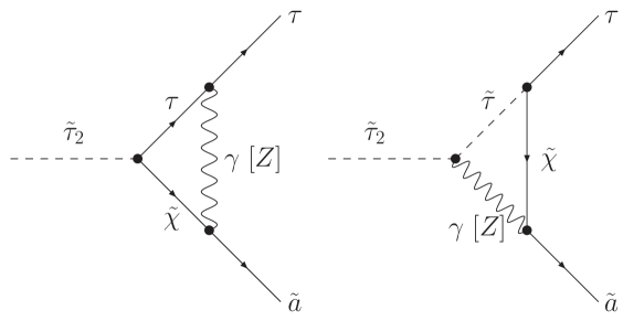
Figure 1: The one-loop diagrams for the decay $\tilde{\tau}_{2}\rightarrow\tau+\tilde{a}$.

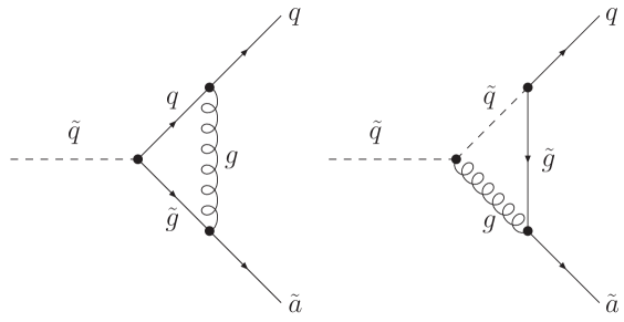
Figure 2: The one-loop diagrams for the decay $\tilde{q}\rightarrow q+\tilde{a}$.

We must further impose the following constraints: ($a$) the predicted axino abundance $\Omega_{\tilde{a}}h^{2}$ should lie in the $95\%$ c.l. range for the CDM abundance in the universe derived by the WMAP satellite wmap , ($b$) both the TP and NTP axinos must become non-relativistic before matter domination so as to contribute to CDM, and ($c$) the NTP axinos should not contribute too much relativistic energy density during BBN since this can destroy its successful predictions. For both $\tilde{\chi}$ or $\tilde{\tau}_{2}$ LOSP, the requirements ($b$) and ($c$) imply that $m_{\tilde{a}}\stackrel{{\scriptstyle>}}{{{}_{\sim}}}100~{}{\rm keV}$ or, equivalently, $T_{\rm r}\stackrel{{\scriptstyle<}}{{{}_{\sim}}}5\times 10^{6}~{}{\rm GeV}$. For large values of the reheat temperature ($T_{\rm r}\stackrel{{\scriptstyle>}}{{{}_{\sim}}}10^{4}~{}{\rm GeV}$), TP of axinos is more efficient than NTP and the cosmologically favored region in parameter space where the requirement ($a$) holds is quite narrow. For smaller $T_{\rm r}$’s, NTP dominates yielding a much wider favored region with $m_{\tilde{a}}\stackrel{{\scriptstyle>}}{{{}_{\sim}}}10~{}{\rm MeV}$. The upper bound on $m_{\tilde{a}}$ increases as $T_{\rm r}$ decreases towards $m_{\tilde{\chi}}$. For $m_{\tilde{q}}\ll m_{\tilde{g}}$, TP of axinos via the process $\tilde{q}\rightarrow q+\tilde{a}$ becomes small2 very efficient leading to a reduction of the upper limit on $T_{\rm r}$. As a result, the cosmologically favored region from NTP is reduced in this case. The Feynman diagrams for the process $\tilde{q}\rightarrow q+\tilde{a}$ are depicted in Fig. 2. The restrictions on the $m_{\tilde{a}}-T_{\rm r}$ plane from axino CDM considerations are presented in Fig. 3.

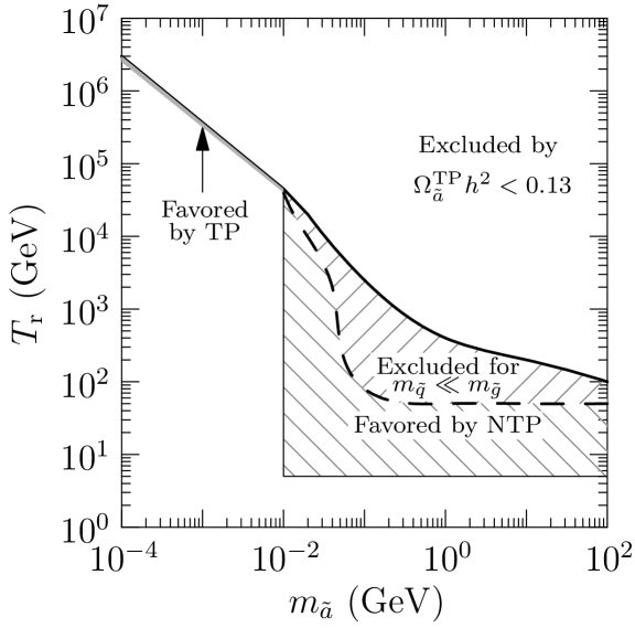
Figure 3: The restrictions on the $m_{\tilde{a}}-T_{\rm r}$ plane from axino CDM considerations for $\tilde{\chi}=\tilde{B}$, $m_{\tilde{\chi}}=100~{}{\rm GeV}$, $m_{\tilde{g}}=m_{\tilde{q}}=1~{}{\rm TeV}$, and $f_{a}=10^{11}~{}{\rm GeV}$. The solid almost diagonal line corresponds to $\Omega_{a}^{\rm TP}h^{2}\approx 0.13$, where $\Omega_{a}^{\rm TP}h^{2}$ is the TP axino abundance. So, the area above this line is cosmologically excluded. The narrow shaded area just below the thin part of this line for $m_{\tilde{a}}\stackrel{{\scriptstyle<}}{{{}_{\sim}}}10~{}{\rm MeV}$ is cosmologically favored by TP. The hatched areas are favored by NTP. For $m_{\tilde{q}}\ll m_{\tilde{g}}$, the solid line is replaced by the dashed one, whose position is strongly dependent on the actual values of $m_{\tilde{q}}$, $m_{\tilde{g}}$ and is only indicative here. The area favored by NTP is then limited only to the “back-hatched” region which lies below the dashed line.

We find small1 that, for the CMSSM, with appropriate choices of $m_{\tilde{a}}$ and $T_{\rm r}$, almost any pair of values for $m_{0}$ and $M_{1/2}$ can be allowed. This holds for both $\tilde{\chi}$ or $\tilde{\tau}_{2}$ as LOSP. However, the required $T_{\rm r}$’s for achieving the WMAP bound on CDM turn out to be quite low ($\stackrel{{\scriptstyle<}}{{{}_{\sim}}}{\rm few}\times 100~{}{\rm GeV}$).

6 Gravitinos

It has been proposed gravitino ; gravitino1 that CDM could also consist of gravitinos. The gravitino $\tilde{G}$ is the superpartner of the graviton and has negative R-parity. It can be the LSP in many cases and, thus, contribute to CDM. In the very CMSSM, its mass $m_{\tilde{G}}$ is fixed by the asymptotic condition $m_{3/2}=m_{0}$. In the general CMSSM, however, it is a free parameter ranging between $100~{}{\rm GeV}$ and $1~{}{\rm TeV}$. It can, thus, very easily be the LSP in this case.

The couplings of the gravitino are suppressed by the Planck scale. The most important of them are given by the dimension-five Lagrangian terms

$$\mathcal{L} = -\frac{1}{\sqrt{2}m_{\rm P}}\mathcal{D}_{\nu}\phi^{i*}\bar{\tilde{\psi}}_{\mu}\gamma^{\nu}\gamma^{\mu}\psi^{i}-\frac{1}{\sqrt{2}m_{\rm P}}\mathcal{D}_{\nu}\phi^{i}\bar{\psi}^{i}\gamma^{\mu}\gamma^{\nu}\tilde{\psi}_{\mu}$$ (28)

$$-\frac{i}{8m_{\rm P}}\bar{\tilde{\psi}}_{\mu}[\gamma^{\nu},\gamma^{\rho}]\gamma^{\mu}\tilde{\lambda}^{a}F^{a}_{\nu\rho},$$

where $\tilde{\psi}_{\mu}$ denotes the gravitino field, $\phi^{i}$ are the complex scalar fields, $\psi^{i}$ are the corresponding chiral fermion fields, $\tilde{\lambda}^{a}$ are the gaugino fields, $m_{\rm P}\simeq 2.44\times 10^{18}~{}{\rm GeV}$ is the reduced Planck scale, and $\mathcal{D}_{\nu}$ denotes the covariant derivative. From these Lagrangian terms, we obtain scalar–fermion–gravitino vertices ($\phi f\tilde{G}$) such as $q\tilde{q}\tilde{G}$, $l\tilde{l}\tilde{G}$, and $H\tilde{H}\tilde{G}$, as well as gaugino–gauge boson–gravitino vertices ($\tilde{\lambda}F\tilde{G}$) such as $g\tilde{g}\tilde{G}$ and $B\tilde{B}\tilde{G}$ (in this section, $l$ and $H$ represent any lepton and Higgs boson respectively).

The gravitinos are thermally produced after reheating by $2\rightarrow 2$ scattering processes involving the above vertices. Such processes are gravitino ; gravitino1

$$g+g\rightarrow\tilde{G}+\tilde{g},\quad g+\tilde{g} \rightarrow \tilde{G}+g,\quad g+\tilde{q}\rightarrow\tilde{G}+q,\quad g+q\rightarrow\tilde{G}+\tilde{q},$$

$$q+\tilde{q}\rightarrow\tilde{G}+g,\quad\tilde{g}+\tilde{g} \rightarrow \tilde{G}+\tilde{g},\quad\tilde{g}+q\rightarrow\tilde{G}+q,\quad\tilde{g}+\tilde{q}\rightarrow\tilde{G}+\tilde{q},$$

$$q+\bar{q} \rightarrow \tilde{G}+\tilde{g},\quad\tilde{q}+\tilde{q}\rightarrow\tilde{G}+\tilde{g}.$$ (29)

There is gravitino1 ; gravitinoNTP also NTP of gravitinos via the decay of the NLSP. For neutralino NLSP, the relevant decay processes are $\tilde{\chi}\rightarrow\tilde{G}+\gamma~{}[{\rm or}~{}Z]$ from the $\tilde{\lambda}F\tilde{G}$ coupling and $\tilde{\chi}\rightarrow\tilde{G}+H$ from the $H\tilde{H}\tilde{G}$ coupling. In the case of $\tilde{\tau}_{2}$ NLSP, the relevant decay process is $\tilde{\tau}_{2}\rightarrow\tau+\tilde{G}$ from the vertex $l\tilde{l}\tilde{G}$. There is an important difference between the NTP of gravitinos and axinos. In the former case, the NLSP has a large lifetime (up to about $10^{8}~{}{\rm sec}$). Consequently, it gives rise mostly to electromagnetic, but also to hadronic showers well after BBN. The electromagnetic showers cause destruction of some light elements (D, ${}^{4}{\rm He}$, ${}^{7}{\rm Li}$) and/or overproduction of ${}^{3}{\rm He}$ and ${}^{6}{\rm Li}$, thereby disturbing BBN. The hadronic showers can also disturb BBN. The overall resulting constraint is gravitinoCmssm very strong allowing only limited regions of the parameter space of the CMSSM lying exclusively in the range where the NLSP is the $\tilde{\tau}_{2}$. Moreover, in these allowed regions, the NTP of gravitinos is not efficient enough to account for the observed CDM abundance for $M_{1/2}\stackrel{{\scriptstyle<}}{{{}_{\sim}}}6~{}{\rm TeV}$. However, we can compensate for the inefficiency of NTP by raising $T_{\rm r}$ to enhance the TP of $\tilde{G}$’s. The relic gravitino abundance from TP, for $m_{\tilde{G}}\ll m_{\tilde{g}}$, is gravitinoTPformula

$$\Omega^{\rm TP}_{\tilde{G}}h^{2}\approx 0.2\left(\frac{T_{\rm r}}{10^{10}~{}{\rm GeV}}\right)\left(\frac{100~{}{\rm GeV}}{m_{\tilde{G}}}\right)\left(\frac{m_{\tilde{g}}(\mu)}{1~{}{\rm TeV}}\right),$$ (30)

where $m_{\tilde{g}}(\mu)$ is the running gluino mass (for the general formula, see Ref. steffen ).

7 Yukawa Quasi-Unification

As already said in Sec. 3, exact YU in the framework of the CMSSM leads to wrong values for $m_{b}$ and, thus, must be corrected. We will now present a model which naturally solves qcdm (see also Refs. balkan ; nova ) this $m_{b}$ problem and discuss the restrictions on its parameter space implied by CDM considerations and other phenomenological constraints. Exact YU can be achieved by embedding the MSSM in a SUSY GUT model with a gauge group containing ${\rm SU(4)}_{c}$ and ${\rm SU(2)}_{\rm R}$. Indeed, assuming that the electroweak Higgs superfields $H_{1}$, $H_{2}$ and the third family right handed quark superfields $t^{c}$, $b^{c}$ form ${\rm SU(2)}_{\rm R}$ doublets, we obtain pana the asymptotic Yukawa coupling relation $h_{t}=h_{b}$ and, hence, large $\tan\beta\sim m_{t}/m_{b}$. Moreover, if the third generation quark and lepton ${\rm SU(2)}_{\rm L}$ doublets [singlets] $q_{3}$ and $l_{3}$ [$b^{c}$ and $\tau^{c}$] form a ${\rm SU(4)}_{c}$ 4-plet [${\bf\bar{4}}$-plet] and the Higgs doublet $H_{1}$ which couples to them is a ${\rm SU(4)}_{c}$ singlet, we get $h_{b}=h_{\tau}$ and the asymptotic relation $m_{b}=m_{\tau}$ follows. The simplest GUT gauge group which contains both ${\rm SU(4)}_{c}$ and ${\rm SU(2)}_{\rm R}$ is the Pati-Salam (PS) group $G_{\rm PS}={\rm SU(4)}_{c}\times{\rm SU(2)}_{\rm L}\times{\rm SU(2)}_{\rm R}$ and we will use it here.

As mentioned, applying YU in the context of the CMSSM and given the experimental values of the top-quark and tau-lepton masses (which naturally restrict $\tan\beta\sim 50$), the resulting value of the $b$-quark mass turns out to be unacceptable. This is due to the fact that, in the large $\tan\beta$ regime, the tree-level $b$-quark mass receives sizeable SUSY corrections pierce ; copw ; susy ; king (about 20$\%$), which have the sign of $\mu$ (with the standard sign convention sugra ) and drive, for $\mu>[<]~{}0$, the corrected $b$-quark mass at $M_{Z}$, $m_{b}(M_{Z})$, well above [somewhat below] its $95\%$ c.l. experimental range

$$2.684~{}{\rm GeV}\stackrel{{\scriptstyle<}}{{{}_{\sim}}}m_{b}(M_{Z})\stackrel{{\scriptstyle<}}{{{}_{\sim}}}3.092~{}{\rm GeV}\quad\mbox{with}\quad\alpha_{s}(M_{Z})=0.1185.$$ (31)

This is derived by appropriately qcdm evolving the corresponding range of $m_{b}(m_{b})$ in the $\overline{MS}$ scheme (i.e. $3.95-4.55~{}{\rm GeV}$) up to $M_{Z}$ in accordance with Ref. baermb . We see that, for both signs of $\mu$, YU leads to an unacceptable $b$-quark mass with the $\mu<0$ case being less disfavored.

A way out of this $m_{b}$ problem can be found qcdm (see also Refs. balkan ; nova ) without having to abandon the CMSSM (in contrast to the usual strategy king ; raby ; baery ; nath ) or YU altogether. We can rather modestly correct YU by including an extra ${\rm SU(4)}_{c}$ non-singlet Higgs superfield with Yukawa couplings to the quarks and leptons. The Higgs ${\rm SU(2)}_{\rm L}$ doublets contained in this superfield can naturally develop wetterich subdominant VEVs and mix with the main electroweak doublets, which are assumed to be ${\rm SU(4)}_{c}$ singlets and form a ${\rm SU(2)}_{\rm R}$ doublet. This mixing can, in general, violate the ${\rm SU(2)}_{\rm R}$ symmetry. Consequently, the resulting electroweak Higgs doublets $H_{1}$, $H_{2}$ do not form a ${\rm SU(2)}_{\rm R}$ doublet and also break the ${\rm SU}(4)_{c}$ symmetry. The required deviation from YU is expected to be more pronounced for $\mu>0$. Despite this, we will study here this case, since the $\mu<0$ case has been excluded cd2 by combining the WMAP restrictions wmap on the CDM in the universe with the experimental results cleo on the inclusive branching ratio ${\rm BR}(b\rightarrow s\gamma)$. The same SUSY GUT model which, for $\mu>0$ and universal boundary conditions, remedies the $m_{b}$ problem leads to a new version jean2 of shifted hybrid inflation jean , which, as the older version jean , avoids monopole overproduction at the end of inflation, but, in contrast to that version, is based only on renormalizable interactions.

In Sec. 7.1, we review the construction of a SUSY GUT model which naturally and modestly violates YU, yielding an appropriate Yukawa quasi-unification condition (YQUC), which is derived in Sec. 7.2. We then outline the resulting CMSSM in Sec. 7.3 and introduce the various cosmological and phenomenological requirements which restrict its parameter space in Sec. 7.4. In Sec. 7.5, we delineate the allowed range of parameters. Finally, in Sec. 7.6, we briefly comment on the new version of shifted hybrid inflation which is realized in this model.

7.1 The PS SUSY GUT Model

We will take the SUSY GUT model of shifted hybrid inflation jean (see also Ref. talks ) as our starting point. It is based on $G_{\rm PS}$, which is the simplest GUT gauge group that can lead to exact YU. The representations under $G_{\rm PS}$ and the global charges of the various matter and Higgs superfields contained in this model are presented in Table 2, which also contains the extra Higgs superfields required for accommodating an adequate violation of YU for $\mu>0$ (see below). The matter superfields are $F_{i}$ and $F^{c}_{i}$ ($i=1,2,3$), while the electroweak Higgs doublets belong to the superfield $h$. So, all the requirements for exact YU are fulfilled. The spontaneous breaking of $G_{\rm PS}$ down to $G_{\rm SM}$ is achieved by the superheavy VEVs ($\sim M_{\rm GUT}$) of the right handed neutrino-type components of a conjugate pair of Higgs superfields $H^{c}$, $\bar{H}^{c}$. The model also contains a gauge singlet $S$ which triggers the breaking of $G_{\rm PS}$, a ${\rm SU(4)}_{c}$ 6-plet $G$ which gives leontaris masses to the right handed down-quark-type components of $H^{c}$, $\bar{H}^{c}$, and a pair of gauge singlets $N$, $\bar{N}$ for solving rsym the $\mu$ problem of the MSSM via a PQ symmetry (for an alternative solution of the $\mu$ problem, see Ref. dvali ). In addition to $G_{\rm PS}$, the model possesses two global ${\rm U(1)}$ symmetries, namely a R and a PQ symmetry, as well as the discrete matter parity symmetry $Z_{2}^{\rm mp}$. Note that global continuous symmetries such as our PQ and R symmetry can effectively arise laz1 from the rich discrete symmetry groups encountered in many compactified string theories (see e.g. Ref. laz2 ). Note that, although the model contains baryon- and lepton-number-violating superpotential terms, the proton is qcdm ; jean practically stable. The baryon asymmetry of the universe is generated via the non-thermal realization origin of the leptogenesis scenario lepto (for recent papers on non-thermal leptogenesis, see e.g. Ref. leptosc ).

Table 2: Superfield Content of the Model

Superfields	Representations	Global
	under $G_{\rm PS}$	Charges
		$R$	$PQ$	$Z^{\rm mp}_{2}$
Matter Superfields
$F_{i}$	$({\bf 4,2,1})$	$1/2$	$-1$	$1$
$F^{c}_{i}$	$({\bf\bar{4},1,2})$	$1/2$	$0$	$-1$
Higgs Superfields
$h$	$({\bf 1,2,2})$	$0$	$1$	$0$
$H^{c}$	$({\bf\bar{4},1,2})$	$0$	$0$	$0$
$\bar{H}^{c}$	$({\bf 4,1,2})$	$0$	$0$	$0$
$S$	$({\bf 1,1,1})$	$1$	$0$	$0$
$G$	$({\bf 6,1,1})$	$1$	$0$	$0$
$N$	$({\bf 1,1,1})$	$1/2$	$-1$	$0$
$\bar{N}$	$({\bf 1,1,1})$	$0$	$1$	$0$
Extra Higgs Superfields
$h^{\prime}$	$({\bf 15,2,2})$	$0$	$1$	$0$
$\bar{h}^{\prime}$	$({\bf 15,2,2})$	$1$	$-1$	$0$
$\phi$	$({\bf 15,1,3})$	$0$	$0$	$0$
$\bar{\phi}$	$({\bf 15,1,3})$	$1$	$0$	$0$

A moderate violation of exact YU can be naturally accommodated in this model by adding a new Higgs superfield $h^{\prime}$ with Yukawa couplings $FF^{c}h^{\prime}$. Actually, (15,2,2) is the only representation of $G_{\rm PS}$, besides (1,2,2), which possesses such couplings to the matter superfields. In order to give superheavy masses to the color non-singlet components of $h^{\prime}$, we need to include one more Higgs superfield $\bar{h}^{\prime}$ with the superpotential coupling $\bar{h}^{\prime}h^{\prime}$, whose coefficient is of the order of $M_{\rm GUT}$.

After the breaking of $G_{\rm PS}$ to $G_{\rm SM}$, the two color singlet ${\rm SU(2)}_{\rm L}$ doublets $h_{1}^{\prime}$, $h_{2}^{\prime}$ contained in $h^{\prime}$ can mix with the corresponding doublets $h_{1}$, $h_{2}$ in $h$. This is mainly due to the terms $\bar{h}^{\prime}h^{\prime}$ and $H^{c}\bar{H}^{c}\bar{h}^{\prime}h$. Actually, since

$$H^{c}\bar{H}^{c}=({\bf\bar{4},1,2})({\bf 4,1,2})=({\bf 15,1,1+3})+\cdots,$$

$$\bar{h}^{\prime}h=({\bf 15,2,2})({\bf 1,2,2})=({\bf 15,1,1+3})+\cdots,$$ (32)

there are two independent couplings of the type $H^{c}\bar{H}^{c}\bar{h}^{\prime}h$ (both suppressed by the string scale $M_{\rm S}\approx 5\times 10^{17}~{}{\rm GeV}$, as they are non-renormalizable). One of these couplings is between the ${\rm SU(2)}_{\rm R}$ singlets in $H^{c}\bar{H}^{c}$ and $\bar{h}^{\prime}h$ and the other between the ${\rm SU(2)}_{\rm R}$ triplets in these combinations. So, we obtain two bilinear terms $\bar{h}_{1}^{\prime}h_{1}$ and $\bar{h}_{2}^{\prime}h_{2}$ with different coefficients, which are suppressed by $M_{\rm GUT}/M_{\rm S}$. These terms together with the terms $\bar{h}_{1}^{\prime}h_{1}^{\prime}$ and $\bar{h}_{2}^{\prime}h_{2}^{\prime}$ from $\bar{h}^{\prime}h^{\prime}$, which have equal coefficients, generate different mixings between $h_{1}$, $h_{1}^{\prime}$ and $h_{2}$, $h_{2}^{\prime}$. Consequently, the resulting electroweak doublets $H_{1}$, $H_{2}$ contain ${\rm SU}(4)_{c}$ violating components suppressed by $M_{\rm GUT}/M_{\rm S}$ and fail to form a ${\rm SU(2)}_{\rm R}$ doublet by an equally suppressed amount. So, YU is naturally and moderately violated. Unfortunately, as it turns out, this violation is not adequately large for correcting the bottom-quark mass within the framework of the CMSSM with $\mu>0$.

In order to allow for a more sizable violation of YU, we further extend the model by including the superfield $\phi$ with the coupling $\phi\bar{h}^{\prime}h$. To give superheavy masses to the color non-singlets in $\phi$, we introduce one more superfield $\bar{\phi}$ with the coupling $\bar{\phi}\phi$, whose coefficient is of order $M_{\rm GUT}$.

The superpotential terms $\bar{\phi}\phi$ and $\bar{\phi}H^{c}\bar{H}^{c}$ imply that, after the breaking of $G_{\rm PS}$ to $G_{\rm SM}$, $\phi$ acquires a VEV of order $M_{\rm GUT}$. The coupling $\phi\bar{h}^{\prime}h$ then generates ${\rm SU(2)}_{\rm R}$ violating unsuppressed bilinear terms between the doublets in $\bar{h}^{\prime}$ and $h$. These terms can overshadow the corresponding ones from the non-renormalizable term $H^{c}\bar{H}^{c}\bar{h}^{\prime}h$. The resulting ${\rm SU(2)}_{\rm R}$ violating mixing of the doublets in $h$ and $h^{\prime}$ is then unsuppressed and we can obtain stronger violation of YU.

7.2 The YQUC

To further analyze the mixing of the doublets in $h$ and $h^{\prime}$, observe that the part of the superpotential corresponding to the symbolic couplings $\bar{h}^{\prime}h^{\prime}$, $\phi\bar{h}^{\prime}h$ is properly written as

$$m{\rm tr}\left(\bar{h}^{\prime}\epsilon h^{\prime\,{\rm T}}\epsilon\right)+p{\rm tr}\left(\bar{h}^{\prime}\epsilon\phi h^{\rm T}\epsilon\right),$$ (33)

where $m$ is a mass parameter of order $M_{\rm GUT}$, $p$ is a dimensionless parameter of order unity, ${\rm tr}$ denotes trace taken with respect to the ${\rm SU(4)}_{\rm c}$ and ${\rm SU(2)}_{\rm L}$ indices, and the superscript T denotes the transpose of a matrix.

After the breaking of $G_{\rm PS}$ to $G_{\rm SM}$, $\phi$ acquires a VEV $\langle\phi\rangle\sim M_{\rm GUT}$. Substituting it by this VEV in the above couplings, we obtain

$${\rm tr}(\bar{h}^{\prime}\epsilon h^{\prime\,{\rm T}}\epsilon)=\bar{h}^{\prime\,{\rm T}}_{1}\epsilon h^{\prime}_{2}+h^{\prime\,{\rm T}}_{1}\epsilon\bar{h}^{\prime}_{2}+\cdots,$$ (34)

$${\rm tr}(\bar{h}^{\prime}\epsilon\phi h^{\rm T}\epsilon)=\frac{\langle\phi\rangle}{\sqrt{2}}{\rm tr}(\bar{h}^{\prime}\epsilon\sigma_{3}h^{\rm T}\epsilon)=\frac{\langle\phi\rangle}{\sqrt{2}}(\bar{h}^{\prime\,{\rm T}}_{1}\epsilon h_{2}-h_{1}^{\rm T}\epsilon\bar{h}^{\prime}_{2}),$$ (35)

where the ellipsis in Eq. (34) contains the colored components of $\bar{h}^{\prime}$, $h^{\prime}$ and $\sigma_{3}={\rm diag}(1,-1)$. Inserting Eqs. (34) and (35) into Eq. (33), we obtain

$$m\bar{h}^{\prime\,{\rm T}}_{1}\epsilon(h^{\prime}_{2}-\alpha h_{2})+m(h^{\prime\,{\rm T}}_{1}+\alpha h^{\rm T}_{1})\epsilon\bar{h}^{\prime}_{2}\quad\mbox{with}\quad\alpha=-\frac{p\langle\phi\rangle}{\sqrt{2}m}.$$ (36)

So, we get two pairs of superheavy doublets with mass $m$. They are predominantly given by

$$\bar{h}^{\prime}_{1},~{}\frac{h^{\prime}_{2}-\alpha h_{2}}{\sqrt{1+|\alpha|^{2}}}\quad{\rm and}\quad\frac{h^{\prime}_{1}+\alpha h_{1}}{\sqrt{1+|\alpha|^{2}}},~{}\bar{h}^{\prime}_{2}.$$ (37)

The orthogonal combinations of $h_{1}$, $h^{\prime}_{1}$ and $h_{2}$, $h^{\prime}_{2}$ constitute the electroweak doublets

$$H_{1}=\frac{h_{1}-\alpha^{*}h^{\prime}_{1}}{\sqrt{1+|\alpha|^{2}}}\quad{\rm and}\quad H_{2}=\frac{h_{2}+\alpha^{*}h^{\prime}_{2}}{\sqrt{1+|\alpha|^{2}}}.$$ (38)

The superheavy doublets in Eq. (37) must have vanishing VEVs, which readily implies that $\langle h_{1}^{\prime}\rangle=-\alpha\langle h_{1}\rangle$ and $\langle h_{2}^{\prime}\rangle=\alpha\langle h_{2}\rangle$. Equation (38) then gives $\langle H_{1}\rangle=(1+|\alpha|^{2})^{1/2}\langle h_{1}\rangle$, $\langle H_{2}\rangle=(1+|\alpha|^{2})^{1/2}\langle h_{2}\rangle$. From the third generation Yukawa couplings $y_{33}F_{3}hF_{3}^{c}$, $2y_{33}^{\prime}F_{3}h^{\prime}F_{3}^{c}$, we obtain

$$m_{t}=|y_{33}\langle h_{2}\rangle+y_{33}^{\prime}\langle h_{2}^{\prime}\rangle|=\left|\frac{1+\rho\alpha/\sqrt{3}}{\sqrt{1+|\alpha|^{2}}}y_{33}\langle H_{2}\rangle\right|,$$ (39)

$$m_{b}=\left|\frac{1-\rho\alpha/\sqrt{3}}{\sqrt{1+|\alpha|^{2}}}y_{33}\langle H_{1}\rangle\right|,~{}m_{\tau}=\left|\frac{1+\sqrt{3}\rho\alpha}{\sqrt{1+|\alpha|^{2}}}y_{33}\langle H_{1}\rangle\right|,$$ (40)

where $\rho=y_{33}^{\prime}/y_{33}$. From Eqs. (39) and (40), we see that YU is now replaced by the YQUC

$$h_{t}:h_{b}:h_{\tau}=(1+c):(1-c):(1+3c)\quad\mbox{with}\quad 0<c=\rho\alpha/\sqrt{3}<1.$$ (41)

For simplicity, we restricted ourselves here to real values of $c$ only which lie between zero and unity, although $c$ is, in general, an arbitrary complex quantity with $|c|\sim 1$.

7.3 The Resulting CMSSM

Below the GUT scale $M_{\rm GUT}$, the particle content of our model reduces to this of MSSM (modulo SM singlets). We assume universal soft SUSY breaking scalar masses $m_{0}$, gaugino masses $M_{1/2}$, and trilinear scalar couplings $A_{0}$ at $M_{\rm GUT}$. Therefore, the resulting MSSM is the so-called CMSSM Cmssm with $\mu>0$ supplemented by the YQUC in Eq. (41). With these initial conditions, we run the MSSM RGEs cdm between $M_{\rm GUT}$ and a common variable SUSY threshold $M_{\rm SUSY}$ (see Sec. 3) determined in consistency with the SUSY spectrum of the model. At $M_{\rm SUSY}$, we impose radiative electroweak symmetry breaking, evaluate the SUSY spectrum and incorporate the SUSY corrections pierce ; susy ; king to the $b$-quark and $\tau$-lepton masses. Note that the corrections to the $\tau$-lepton mass (almost 4$\%$) lead cd2 to a small reduction of $\tan\beta$. From $M_{\rm SUSY}$ to $M_{Z}$, the running of gauge and Yukawa coupling constants is continued using the SM RGEs.

For presentation purposes, $M_{1/2}$ and $m_{0}$ can be replaced cdm by the LSP mass $m_{\rm LSP}$ and the relative mass splitting between this particle and the lightest stau $\Delta_{\tilde{\tau}_{2}}=(m_{\tilde{\tau}_{2}}-m_{\rm LSP})/m_{\rm LSP}$ (recall that $\tilde{\tau}_{2}$ is the NLSP in this case). For simplicity, we restrict this presentation to the $A_{0}=0$ case (for $A_{0}\neq 0$ see Refs. qcdm ; mario ). So, our input parameters are $m_{\rm LSP}$, $\Delta_{\tilde{\tau}_{2}}$, $c$, and $\tan\beta$.

For any given $m_{b}(M_{Z})$ in the range in Eq. (31) and with fixed $m_{t}(m_{t})=166~{}{\rm GeV}$ and $m_{\tau}(M_{Z})=1.746~{}{\rm GeV}$, we can determine the parameters $c$ and $\tan\beta$ at $M_{\rm SUSY}$ so that the YQUC in Eq. (41) is satisfied. We are, thus, left with $m_{\rm LSP}$ and $\Delta_{\tilde{\tau}_{2}}$ as free parameters.

7.4 Cosmological and Phenomenological Constraints

Restrictions on the parameters of our model can be derived by imposing a number of cosmological and phenomenological requirements (for similar recent analyses, see Refs. baery ; nath ; spanos ). These constraints result from

$\bullet$ CDM Considerations. As discussed in Sec. 3, in the context of the CMSSM, the LSP can be the lightest neutralino which is an almost pure bino. It naturally arises goldberg as a CDM candidate. We require its relic abundance, $\Omega_{\rm LSP}h^{2}$, not to exceed the $95\%$ c.l. upper bound on the CDM abundance derived wmap by WMAP:

$$\Omega_{\rm CDM}h^{2}\stackrel{{\scriptstyle<}}{{{}_{\sim}}}0.13.$$ (42)

We calculate $\Omega_{\rm LSP}h^{2}$ using micrOMEGAs micro , which is certainly one of the most complete publicly available codes. Among other things, it includes all possible coannihilation processes ellis2 and one-loop QCD corrections width to the Higgs decay widths and couplings to fermions.

$\bullet$ Branching Ratio of $b\rightarrow s\gamma$. Taking into account the experimental results of Ref. cleo on this ratio, ${\rm BR}(b\rightarrow s\gamma)$, and combining qcdm appropriately the experimental and theoretical errors involved, we obtain the $95\%$ c.l. range

$$1.9\times 10^{-4}\stackrel{{\scriptstyle<}}{{{}_{\sim}}}{\rm BR}(b\rightarrow s\gamma)\stackrel{{\scriptstyle<}}{{{}_{\sim}}}4.6\times 10^{-4}.$$ (43)

Although there exist more recent experimental data babar on the branching ratio of $b\rightarrow s\gamma$, we do not use them here. The reason is that these data do not separate the theoretical errors from the experimental ones and, thus, the derivation of the $95\%$ c.l. range is quite ambiguous. In any case, the $95\%$ c.l. limits obtained in Ref. babarellis on the basis of these latest measurements are not terribly different from the ones quoted in Eq. (43). In view of this and the fact that, in our case, the restrictions from ${\rm BR}(b\rightarrow s\gamma)$ are overshadowed by other constraints (see Sec. 7.5), we limit ourselves to the older data. We compute ${\rm BR}(b\rightarrow s\gamma)$ by using an updated version of the relevant calculation contained in the micrOMEGAs package micro . In this code, the SM contribution is calculated following Ref. kagan . The charged Higgs ($H^{\pm}$) contribution is evaluated by including the next-to-leading order (NLO) QCD corrections nlo and $\tan\beta$ enhanced contributions nlo . The dominant SUSY contribution includes resummed NLO SUSY QCD corrections nlo , which hold for large $\tan\beta$.

$\bullet$ Muon Anomalous Magnetic Moment. The deviation, $\delta a_{\mu}$, of the measured value of $a_{\mu}$ from its predicted value in the SM, $a^{\rm SM}_{\mu}$, can be attributed to SUSY contributions, which are calculated by using the micrOMEGAs routine gmuon . The calculation of $a^{\rm SM}_{\mu}$ is not yet stabilized mainly because of the instability of the hadronic vacuum polarization contribution. According to recent calculations (see e.g. Refs. davier ; vainshtein ), there is still a considerable discrepancy between the findings based on the $e^{+}e^{-}$ annihilation data and the ones based on the $\tau$-decay data. Taking into account the results of Ref. davier and the experimental measurement of $a_{\mu}$ reported in Ref. muon , we get the following $95\%$ c.l. ranges:

$$-0.53\times 10^{-10}\stackrel{{\scriptstyle<}}{{{}_{\sim}}} \delta a_{\mu} \stackrel{{\scriptstyle<}}{{{}_{\sim}}}44.7\times 10^{-10},~{}\quad\mbox{$e^{+}e^{-}$-based};$$ (44)

$$\vspace*{19pt}-13.6\times 10^{-10}\stackrel{{\scriptstyle<}}{{{}_{\sim}}} \delta a_{\mu} \stackrel{{\scriptstyle<}}{{{}_{\sim}}}28.4\times 10^{-10},\quad\mbox{$\tau$-based}.$$ (45)

Following the common practice spanos , we adopt the restrictions to parameters induced by Eq. (44), since Eq. (45) is considered as quite oracular, due to poor $\tau$-decay data. It is true that there exist more recent experimental data muonn on $a_{\mu}$ than the ones we considered and more updated estimates of $\delta a_{\mu}$ than the one in Ref. davier (see e.g. Ref. vainshtein ). However, only the $95\%$ c.l. upper limit on $\delta a_{\mu}$ enters into our analysis here and its new values are not very different from the one in Eq. (44).

$\bullet$ Collider Bounds. Here, as it turns out, the only relevant collider bound is the $95\%$ c.l. LEP lower bound higgs on the mass of the lightest $CP$-even neutral Higgs boson $h$:

$$m_{h}\stackrel{{\scriptstyle>}}{{{}_{\sim}}}114.4~{}{\rm GeV}.$$ (46)

The SUSY corrections to the lightest $CP$-even Higgs boson mass $m_{h}$ are calculated at two loops by using the FeynHiggsFast program fh included in the micrOMEGAs code micro .

7.5 The Allowed Parameter Space

We will now try to delineate the parameter space of our model with $\mu>0$ which is consistent with the constraints in Sec. 7.4. The restrictions on the $m_{\rm LSP}-\Delta_{\tilde{\tau}_{2}}$ plane, for $A_{0}=0$ and the central values of $\alpha_{s}(M_{Z})=0.1185$ and $m_{b}(M_{Z})=2.888~{}{\rm GeV}$, are indicated in Fig. 4 by solid lines, while the upper bound on $m_{\rm LSP}$ from Eq. (42), for $m_{b}(M_{Z})=2.684~{}[3.092]~{}{\rm GeV}$, is depicted by a dashed [dotted] line. We observe the following:

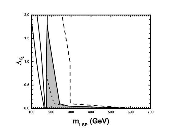
Figure 4: The various restrictions on the $m_{\rm LSP}-\Delta_{\tilde{\tau}_{2}}$ plane for $\mu>0$, $A_{0}=0$, and $\alpha_{s}(M_{Z})=0.1185$. From left to right, the solid lines depict the lower bounds on $m_{\rm LSP}$ from $\delta a_{\mu}<44.7\times 10^{-10}$, ${\rm BR}(b\rightarrow s\gamma)>1.9\times 10^{-4}$, and $m_{h}>114.4~{}{\rm GeV}$ and the upper bound on $m_{\rm LSP}$ from $\Omega_{\rm LSP}h^{2}<0.13$ for $m_{b}(M_{Z})=2.888~{}{\rm GeV}$. The dashed [dotted] line depicts the upper bound on $m_{\rm LSP}$ from $\Omega_{\rm LSP}h^{2}<0.13$ for $m_{b}(M_{Z})=2.684~{}[3.092]~{}{\rm GeV}$. The allowed area for $m_{b}(M_{Z})=2.888~{}{\rm GeV}$ is shaded.

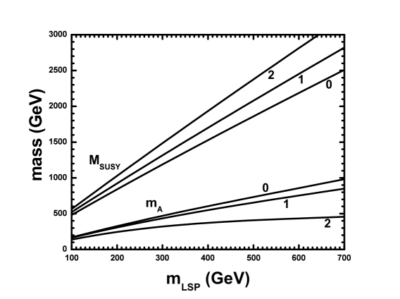
Figure 5: The mass parameters $m_{A}$ and $M_{\rm SUSY}$ versus $m_{\rm LSP}$ for various values of $\Delta_{\tilde{\tau}_{2}}$, which are indicated on the curves. We take $\mu>0$, $A_{0}=0$, $m_{b}(M_{Z})=2.888~{}{\rm GeV}$, and $\alpha_{s}(M_{Z})=0.1185$.

• The lower bounds on $m_{\rm LSP}$ are not so sensitive to the variations of $m_{b}(M_{Z})$.

• The lower bound on $m_{\rm LSP}$ from Eq. (46) overshadows all the other lower bounds on this mass.

• The upper bound on $m_{\rm LSP}$ from Eq. (42) is very sensitive to the variations of $m_{b}(M_{Z})$. In particular, one notices the extreme sensitivity of the almost vertical part of the corresponding line, where the LSP annihilation via an $A$-boson exchange in the s-channel is lah by far the dominant process, since $m_{A}$, which is smaller than $2m_{\rm LSP}$, is always very close to it as seen from Fig. 5. This sensitivity can be understood from Fig. 6, where $m_{A}$ is depicted versus $m_{\rm LSP}$ for various $m_{b}(M_{Z})$’s. We see that, as $m_{b}(M_{Z})$ decreases, $m_{A}$ increases and approaches $2m_{\rm LSP}$. The $A$-pole annihilation is then enhanced and $\Omega_{\rm LSP}h^{2}$ is drastically reduced causing an increase of the upper bound on $m_{\rm LSP}$.

  

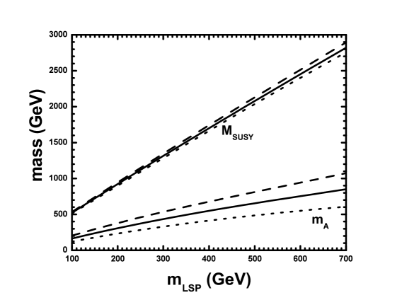
  Figure 6: The mass parameters $m_{A}$ and $M_{\rm SUSY}$ as functions of $m_{\rm LSP}$ for $\mu>0$, $A_{0}=0$, $\Delta_{\tilde{\tau}_{2}}=1$, $\alpha_{s}(M_{Z})=0.1185$, and with $m_{b}(M_{Z})=2.684~{}{\rm GeV}$ (dashed lines), $3.092~{}{\rm GeV}$ (dotted lines), or $2.888~{}{\rm GeV}$ (solid lines).

• For low $\Delta_{\tilde{\tau}_{2}}$’s, bino-stau coannihilations ellis2 take over leading to a very pronounced reduction of the LSP relic abundance $\Omega_{\rm LSP}h^{2}$, thereby enhancing the upper limit on $m_{\rm LSP}$. So, we obtain the almost horizontal tail of the allowed region in Fig. 4.

For $\mu>0$, $A_{0}=0$, $\alpha_{s}(M_{Z})=0.1185$ and $m_{b}(M_{Z})=2.888~{}{\rm GeV}$, we find the following allowed ranges of parameters:

$$176~{}{\rm GeV}\stackrel{{\scriptstyle<}}{{{}_{\sim}}}m_{\rm LSP}\stackrel{{\scriptstyle<}}{{{}_{\sim}}}615~{}{\rm GeV},\quad 0\stackrel{{\scriptstyle<}}{{{}_{\sim}}}\Delta_{\tilde{\tau}_{2}}\stackrel{{\scriptstyle<}}{{{}_{\sim}}}1.8,$$

$$58\stackrel{{\scriptstyle<}}{{{}_{\sim}}}\tan\beta\stackrel{{\scriptstyle<}}{{{}_{\sim}}}59,\quad 0.14\stackrel{{\scriptstyle<}}{{{}_{\sim}}}c\stackrel{{\scriptstyle<}}{{{}_{\sim}}}0.17.$$ (47)

The splitting between the bottom (or tau) and top Yukawa coupling constants $\delta h\equiv-(h_{b}-h_{t})/h_{t}=(h_{\tau}-h_{t})/h_{t}=2c/(1+c)$ ranges between 0.25 and 0.29.

7.6 The New Shifted Hybrid Inflation

It is interesting to note that our SUSY GUT model gives rise jean2 naturally to a modified version of shifted hybrid inflation jean . Hybrid inflation linde , which is certainly one of the most promising inflationary scenarios, uses two real scalars: one which provides the vacuum energy density for driving inflation and a second which is the slowly varying field during inflation. This scheme, which is naturally incorporated hybrid in SUSY GUTs (for an updated review, see Ref. senoguz ), in its standard realization has the following property pana1 : if the GUT gauge symmetry breaking predicts topological defects such as magnetic monopoles monopole , cosmic strings strings , or domain walls wall , these defects are copiously produced at the end of inflation. In the case of monopoles or walls, this leads to a cosmological catastrophe kibble . The breaking of the $G_{\rm PS}$ symmetry predicts the existence of doubly charged monopoles laz3 . So, any PS SUSY GUT model incorporating the standard realization of SUSY hybrid inflation would be unacceptable. One way to remedy this is to invoke thermal1 thermal inflation thermal2 to dilute the primordial monopoles well after their production. Alternatively, we can construct variants of the standard SUSY hybrid inflationary scenario such as smooth pana1 or shifted jean hybrid inflation which do not suffer from the monopole overproduction problem. In the latter scenario, we generate jean a shifted inflationary trajectory so that $G_{\rm PS}$ is already broken during inflation. This could be achieved jean in our SUSY GUT model even before the introduction of the extra Higgs superfields, but only by utilizing non-renormalizable terms. The inclusion of $h^{\prime}$ and $\bar{h}^{\prime}$ does not change this situation. The inclusion of $\phi$ and $\bar{\phi}$, however, very naturally gives rise jean2 to a shifted path, but now with renormalizable interactions alone.

8 Conclusions

We showed that particle physics provides us with a number of candidate particles out of which the CDM of the universe can be made. These particles are not invented solely for explaining the CDM, but they are naturally there in various particle physics models. We discussed in some detail the major candidates which are the axion, the lightest neutralino, the axino, and the gravitino. The last three particles exist only in SUSY theories and can be stable provided that they are the LSP.

The axion is a pseudo Nambu-Goldstone boson associated with the spontaneous breaking of a PQ symmetry. This is a global anomalous ${\rm U}(1)$ symmetry invoked to solve the strong $CP$ problem. It is, actually, the most natural solution to this problem which is available at present. The axions are extremely light particles and are generated at the QCD phase transition carrying zero momentum. We argued that these particles can easily provide the CDM in the universe. However, if the PQ field emerges with non-zero value at the end of inflation, they lead to isocurvature perturbations, which, for superheavy inflationary scales, are too strong to be compatible with the recent results of the WMAP satellite on the CMBR anisotropies.

The most popular CDM candidate is, certainly, the lightest neutralino which is present in all SUSY models and can be the LSP for a wide range of parameters. We considered it within the simplest SUSY framework which is the MSSM whose salient properties were summarized. We used exclusively the constrained version of MSSM which is known as CMSSM and is based on universal boundary conditions. In this case, the lightest neutralino is an almost pure bino, whereas the NLSP is the lightest stau. We sketched the calculation of the neutralino relic abundance in the universe paying particular attention not only to the neutralino pair annihilations, but to the neutralino-stau coannihilations too. It is very important for the accuracy of the calculation to treat poles and final-state thresholds properly and include the one-loop QCD corrections to the Higgs boson decay widths and the fermion masses. We find that two effects help us reduce the neutralino relic abundance and satisfy the WMAP constraint on CDM: the resonantly enhanced neutralino pair annihilation via an $A$-pole exchange in the s-channel, which appears in the large $\tan\beta$ regime, and the strong neutralino-stau coannihilation, which is achieved when these particles are almost degenerate in mass.

The axino, which is the SUSY partner of the axion, can also be the LSP in many cases since its mass is a strongly model-dependent parameter in the CMSSM. It is produced thermally by 2-body scattering or decay processes in the thermal bath, or non-thermally by the decay of sparticles which are already frozen out of thermal equilibrium. For small axino masses, TP is more important yielding a very narrow favored region in the parameter space. For larger axino masses, however, NTP is more efficient and the favored region in the parameter space becomes considerably wider. One finds that, in the case of the CMSSM, almost any point on the $m_{0}-M_{1/2}$ plane can be allowed by axino CDM considerations. The required reheat temperatures though are quite small ($\stackrel{{\scriptstyle<}}{{{}_{\sim}}}{\rm few}\times 100~{}{\rm GeV}$).

The mass of the gravitino is a practically free parameter in the CMSSM. So, the gravitino can easily be the LSP and, in principle, contribute to the CDM of the universe. It is produced thermally by 2-body scattering processes in the thermal bath as well as non-thermally by the decay of the NLSP, which can be either the neutralino or the stau. In contrast to the axino case, however, the NLSP can now have quite a long lifetime. The electromagnetic showers resulting from the NLSP decay can destroy the successful predictions of BBN. So, we obtain strong constraints which allow only very limited regions of the parameter space of the CMSSM. As it turns out, NTP in these regions is not efficient enough to account for CDM. We can, however, make these regions cosmologically favored by raising $T_{\rm r}$ to enhance TP of gravitinos.

We studied the CMSSM with $\mu>0$ and $A_{0}=0$ applying a YQUC which originates from a PS SUSY GUT model. This condition yields an adequate deviation from YU which allows an acceptable $m_{b}(M_{Z})$. We, also, imposed the constraints from the CDM in the universe, $b\rightarrow s\gamma$, $\delta\alpha_{\mu}$ and $m_{h}$. We found that there exists a wide and natural range of CMSSM parameters which is consistent with all the above constraints. The parameter $\tan\beta$ ranges between about 58 and 59 and the asymptotic splitting between the bottom (or tau) and the top Yukawa coupling constants varies in the range $25-29\%$ for central values of $m_{b}(M_{Z})$ and $\alpha_{s}(M_{Z})$. The predicted LSP mass can be as low as about $176~{}{\rm GeV}$. Moreover, the model resolves the $\mu$ problem of MSSM, predicts stable proton, generates the baryon asymmetry of the universe via primordial leptogenesis, and gives rise to a new version of shifted hybrid inflation which is based solely on renormalizable interactions.

References

- (1) C.L. Bennett et al: Astrophys. J. Suppl. 148, 1 (2003); D.N. Spergel et al: ibid. 148, 175 (2003)
- (2) W.L. Freedman et al: Astrophys. J. 553, 47 (2001)
- (3) D.V. Ahluwalia-Khalilova, D. Grumiller: Phys. Rev. D 72, 067701 (2005); J. Cosmol. Astropart. Phys. 07, 012 (2005); M. Cirelli, N. Fornengo, A. Strumia: hep-ph/0512090
- (4) R. Peccei, H. Quinn: Phys. Rev. Lett. 38, 1440 (1977); S. Weinberg: ibid. 40, 223 (1978); F. Wilczek: ibid. 40, 279 (1978)
- (5) D.S.P. Dearborn, D.N. Schramm, G. Steigman: Phys. Rev. Lett. 56, 26 (1986)
- (6) J. Preskill, M.B. Wise, F. Wilczek: Phys. Lett. B 120, 127 (1983); L.F. Abbott, P. Sikivie: ibid. 120, 133 (1983)
- (7) M. Dine, W. Fischler: Phys. Lett. B 120, 137 (1983)
- (8) P.J. Steinhardt, M.S. Turner: Phys. Lett. B 129, 51 (1983); K. Yamamoto: ibid. 161, 289 (1985)
- (9) G. Lazarides, C. Panagiotakopoulos, Q. Shafi: Phys. Lett. B 192, 323 (1987); G. Lazarides, R.K. Schaefer, D. Seckel, Q. Shafi: Nucl. Phys. B346, 193 (1990)
- (10) K. Choi, E.J. Chun, J.E. Kim: Phys. Lett. B 403, 209 (1997); K. Dimopoulos, G. Lazarides: Phys. Rev. D 73, 023525 (2006)
- (11) A.H. Guth: Phys. Rev. D 23, 347 (1981). For a recent review see G. Lazarides: Lect. Notes Phys. 592, 351 (2002)
- (12) P. Sikivie: Phys. Rev. Lett. 48, 1156 (1982); G. Lazarides, Q. Shafi: Phys. Lett. B 115, 21 (1982); H. Georgi, M.B. Wise: ibid. 116, 123 (1982)
- (13) M.S. Turner: Phys. Rev. D 33, 889 (1986)
- (14) L. Campanelli, M. Giannotti: astro-ph/0512458
- (15) H.V. Peiris et al: Astrophys. J. Suppl. 148, 213 (2003)
- (16) C. Gordon, A. Lewis: Phys. Rev. D 67, 123513 (2003); P. Crotty, J. García-Bellido, J. Lesgourgues, A. Riazuelo: Phys. Rev. Lett. 91, 171301 (2003); C. Gordon, K.A. Malik: Phys. Rev. D 69, 063508 (2004); M. Bucher, J. Dunkley, P.G. Ferreira, K. Moodley, C. Skordis: Phys. Rev. Lett. 93, 081301 (2004); K. Moodley, M. Bucher, J. Dunkley, P.G. Ferreira, C. Skordis: Phys. Rev. D 70, 103520 (2004); M. Beltrán, J. García-Bellido, J. Lesgourgues, A. Riazuelo: ibid. 70, 103530 (2004)
- (17) K. Dimopoulos, G. Lazarides, D. Lyth, R. Ruiz de Austri: J. High Energy Phys. 05, 057 (2003); G. Lazarides, R. Ruiz de Austri, R. Trotta: Phys. Rev. D 70, 123527 (2004); G. Lazarides: Nucl. Phys. B (Proc. Sup.) 148, 84 (2005)
- (18) G.L. Kane, C. Kolda, L. Roszkowski, J.D. Wells: Phys. Rev. D 49, 6173 (1994)
- (19) J.R. Ellis, K.A. Olive, Y. Santoso, V.C. Spanos: Phys. Rev. D 70, 055005 (2004)
- (20) B. Ananthanarayan, G. Lazarides, Q. Shafi: Phys. Rev. D 44, 1613 (1991); Phys. Lett. B 300, 245 (1993). For a more recent update see U. Sarid: hep-ph/9610341 (In: Snowmass 1996, New Directions for High-Energy Physics)
- (21) M.E. Gómez, G. Lazarides, C. Pallis: Phys. Rev. D 61, 123512 (2000); Phys. Lett. B 487, 313 (2000)
- (22) M. Drees, M.M. Nojiri: Phys. Rev. D 45, 2482 (1992)
- (23) V. Barger, M. S. Berger, P. Ohmann: Phys. Rev. D 49, 4908 (1994); M. Drees, M.M. Nojiri: Nucl. Phys. B369, 54 (1992); M. Olechowski, S. Pokorski: ibid. B404, 590 (1993)
- (24) D. Pierce, J. Bagger, K. Matchev, R. Zhang: Nucl. Phys. B491, 3 (1997)
- (25) G. Gamberini, G. Ridolfi, F. Zwirner: Nucl. Phys. B331, 331 (1990)
- (26) H. Baer, C. Chen, M. Drees, F. Paige, X. Tata: Phys. Rev. Lett. 79, 986 (1997)
- (27) F.M. Borzumati, M. Olechowski, S. Pokorski: Phys. Lett. B 349, 311 (1995)
- (28) H. Baer, M. Brhlik, D. Castaño, X. Tata: Phys. Rev. D 58, 015007 (1998)
- (29) K. Griest, D. Seckel: Phys. Rev. D 43, 3191 (1991)
- (30) C. Pallis: Astropart. Phys. 21, 689 (2004); J. Cosmol. Astropart. Phys. 10, 015 (2005); hep-ph/0510234
- (31) M. Drees, M.M. Nojiri: Phys. Rev. D 47, 376 (1993); M. Drees: hep-ph/9703260
- (32) J. Ellis, T. Falk, K.A. Olive: Phys. Lett. B 444, 367 (1998); J. Ellis, T. Falk, G. Ganis, K.A. Olive, M. Schmitt: Phys. Rev. D 58, 095002 (1998)
- (33) J. Ellis, T. Falk, K.A. Olive, M. Srednicki: Astropart. Phys. 13, 181 (2000), (E) ibid. 15, 413 (2001)
- (34) E.W. Kolb, M.S. Turner: The Early Universe (Addison-Wesley, Redwood City CA 1990)
- (35) K. Griest, M. Kamionkowski, M.S. Turner: Phys. Rev. D 41, 3565 (1990)
- (36) P. Gondolo, G. Gelmini: Nucl. Phys. B360, 145 (1991)
- (37) T. Falk, K.A. Olive, M. Srednicki: Phys. Lett. B 339, 248 (1994); J. Edsjö, P. Gondolo: Phys. Rev. D 56, 1879 (1997)
- (38) T. Nihei, L. Roszkowski, R. Ruiz de Austri: J. High Energy Phys. 03, 031 (2002)
- (39) M.E. Gómez, G. Lazarides, C. Pallis: Nucl. Phys. B638, 165 (2002)
- (40) T. Nihei, L. Roszkowski, R. Ruiz de Austri: J. High Energy Phys. 07, 024 (2002)
- (41) V.D. Barger, C. Kao: Phys. Rev. D 57, 3131 (1998)
- (42) J.R. Ellis, T. Falk, G. Ganis, K.A. Olive, M. Srednicki: Phys. Lett. B 510, 236 (2001); L. Roszkowski, R. Ruiz de Austri, T. Nihei: J. High Energy Phys. 08, 024 (2001); A.B. Lahanas, D.V. Nanopoulos, V.C. Spanos: hep-ph/0211286 (In: Oulu 2002, Beyond the Desert)
- (43) A. Djouadi, J. Kalinowski, M. Spira: Comput. Phys. Commun. 108, 56 (1998)
- (44) G. Bélanger, F. Boudjema, A. Pukhov, A. Semenov: Comput. Phys. Commun. 149, 103 (2002)
- (45) P. Gondolo, J. Edsjö, L. Bergström, P. Ullio, E.A. Baltz: astro-ph/0012234 (In: York 2000, The Identification of Dark Matter)
- (46) L. Covi, J.E. Kim, L. Roszkowski: Phys. Rev. Lett. 82, 4180 (1999); L. Covi, H.-B. Kim, J.E. Kim, L. Roszkowski: J. High Energy Phys. 05, 033 (2001); A. Brandenburg, F.D. Steffen: J. Cosmol. Astropart. Phys. 08, 008 (2004)
- (47) L. Roszkowski: hep-ph/0102325 (In: York 2000, The Identification of Dark Matter); J.E. Kim: astro-ph/0205146 (In: Cape Town 2002, Dark Matter in Astro- and Particle Physics)
- (48) K. Rajagopal, M.S. Turner, F. Wilczek: Nucl. Phys. B358, 447 (1991); E.J. Chun, J.E. Kim, H.P. Nilles: Phys. Lett. B 287, 123 (1992)
- (49) L. Covi, L. Roszkowski, R. Ruiz de Austri, M. Small: J. High Energy Phys. 06, 003 (2004); A. Brandenburg, L. Covi, K. Hamaguchi, L. Roszkowski, F.D. Steffen: Phys. Lett. B 617, 99 (2005)
- (50) L. Covi, L. Roszkowski, M. Small: J. High Energy Phys. 07, 023 (2002)
- (51) J. Ellis, J.E. Kim, D. Nanopoulos: Phys. Lett. B 145, 181 (1984); T. Moroi, H. Murayama, M. Yamaguchi: ibid. 303, 289 (1993)
- (52) M. Bolz, W. Buchmüller, M. Plümacher: Phys. Lett. B 443, 209 (1998)
- (53) E. Holtmann, M. Kawasaki, K. Kohri, T. Moroi: Phys. Rev. D 60, 023506 (1999); T. Gherghetta, G.F. Giudice, A. Riotto: Phys. Lett. B 446, 28 (1999); T. Asaka, K. Hamaguchi, K. Suzuki: ibid. 490, 136 (2000); J.L. Feng, A. Rajaraman, F. Takayama: Phys. Rev. Lett. 91, 011302 (2003); Phys. Rev. D 68, 063504 (2003); J.L. Feng, S. Su, F. Takayama: ibid. 70, 063514 (2004); ibid. 70, 075019 (2004)
- (54) L. Roszkowski, R. Ruiz de Austri, K.-Y. Choi: J. High Energy Phys. 08, 080 (2005); D.G. Cerdeno, K.-Y. Choi, K. Jedamzik, L. Roszkowski, R. Ruiz de Austri: hep-ph/0509275
- (55) M. Bolz, A. Brandenburg, W. Buchmüller: Nucl. Phys. B606, 518 (2001)
- (56) F.D. Steffen: hep-ph/0507003
- (57) G. Lazarides, C. Pallis: hep-ph/0404266 (In: Vrnjacka Banja 2003, Mathematical, Theoretical and Phenomenological Challenges beyond the Standard Model)
- (58) G. Lazarides, C. Pallis: hep-ph/0406081
- (59) G. Lazarides, C. Panagiotakopoulos: Phys. Lett. B 337, 90 (1994); S. Khalil, G. Lazarides, C. Pallis: ibid. 508, 327 (2001)
- (60) L. Hall, R. Rattazzi, U. Sarid: Phys. Rev. D 50, 7048 (1994); M. Carena, M. Olechowski, S. Pokorski, C.E.M. Wagner: Nucl. Phys. B426, 269 (1994)
- (61) M. Carena, D. Garcia, U. Nierste, C.E.M. Wagner: Nucl. Phys. B577, 88 (2000)
- (62) S.F. King, M. Oliveira: Phys. Rev. D 63, 015010 (2001)
- (63) S. Abel et al. (SUGRA Working Group Collaboration): hep-ph/0003154
- (64) H. Baer, J. Ferrandis, K. Melnikov, X. Tata: Phys. Rev. D 66, 074007 (2002)
- (65) T. Blažek, R. Dermíšek, S. Raby: Phys. Rev. Lett. 88, 111804 (2002); Phys. Rev. D 65, 115004 (2002)
- (66) D. Auto et al: J. High Energy Phys. 06, 023 (2003)
- (67) U. Chattopadhyay, A. Corsetti, P. Nath: Phys. Rev. D 66, 035003 (2002); C. Pallis: Nucl. Phys. B678, 398 (2004)
- (68) G. Lazarides, Q. Shafi, C. Wetterich: Nucl. Phys. B181, 287 (1981); G. Lazarides, Q. Shafi: ibid. B350, 179 (1991)
- (69) M.E. Gómez, G. Lazarides, C. Pallis: Phys. Rev. D 67, 097701 (2003); C. Pallis, M.E. Gómez: hep-ph/0303098
- (70) R. Barate et al. (ALEPH Collaboration): Phys. Lett. B 429, 169 (1998); K. Abe et al. (BELLE Collaboration): ibid. 511, 151 (2001); S. Chen et al. (CLEO Collaboration): Phys. Rev. Lett. 87, 251807 (2001)
- (71) R. Jeannerot, S. Khalil, G. Lazarides: J. High Energy Phys. 07, 069 (2002)
- (72) R. Jeannerot, S. Khalil, G. Lazarides, Q. Shafi: J. High Energy Phys. 10, 012 (2000)
- (73) G. Lazarides: hep-ph/0011130 (In: Cascais 2000, Recent Developments in Particle Physics and Cosmology); R. Jeannerot, S. Khalil, G. Lazarides: hep-ph/0106035 (In: Cairo 2001, High Energy Physics)
- (74) I. Antoniadis, G.K. Leontaris: Phys. Lett. B 216, 333 (1989)
- (75) G. Lazarides, Q. Shafi: Phys. Rev. D 58, 071702 (1998)
- (76) G.R. Dvali, G. Lazarides, Q. Shafi: Phys. Lett. B 424, 259 (1998)
- (77) G. Lazarides, C. Panagiotakopoulos, Q. Shafi: Phys. Rev. Lett. 56, 432 (1986)
- (78) N. Ganoulis, G. Lazarides, Q. Shafi: Nucl. Phys. B323, 374 (1989); G. Lazarides, Q. Shafi: ibid. B329, 182 (1990)
- (79) G. Lazarides, Q. Shafi: Phys. Lett. B 258, 305 (1991)
- (80) M. Fukugita, T. Yanagida: Phys. Lett. B 174, 45 (1986)
- (81) G. Lazarides: Phys. Lett. B 452, 227 (1999); G. Lazarides, N.D. Vlachos: ibid. 459, 482 (1999); T. Dent, G. Lazarides, R. Ruiz de Austri: Phys. Rev. D 69, 075012 (2004); ibid. 72, 043502 (2005)
- (82) M.E. Gómez, C. Pallis: hep-ph/0303094 (In: Hamburg 2002, Supersymmetry and Unification of Fundamental Interactions)
- (83) J. Ellis, K.A. Olive, Y. Santoso, V.C. Spanos: Phys. Lett. B 565, 176 (2003); A.B. Lahanas, D.V. Nanopoulos: ibid. 568, 55 (2003); H. Baer, C. Balázs: J. Cosmol. Astropart. Phys. 05, 006 (2003); U. Chattopadhyay, A. Corsetti, P. Nath: Phys. Rev. D 68, 035005 (2003)
- (84) H. Goldberg: Phys. Rev. Lett. 50, 1419 (1983); J.R. Ellis, J.S. Hagelin, D.V. Nanopoulos, K.A. Olive, M. Srednicki: Nucl. Phys. B238, 453 (1984)
- (85) B. Aubert et al. (BABAR Collaboration): hep-ex/0207074; hep-ex/0207076
- (86) J.R. Ellis, S. Heinemeyer, K.A. Olive, G. Weiglein: J. High Energy Phys. 02, 013 (2005)
- (87) A.L. Kagan, M. Neubert: Eur. Phys. J. C 7, 5 (1999); P. Gambino, M. Misiak: Nucl. Phys. B611, 338 (2001)
- (88) M. Ciuchini, G. Degrassi, P. Gambino, G. Giudice: Nucl. Phys. B527, 21 (1998); G. Degrassi, P. Gambino, G.F. Giudice: J. High Energy Phys. 12, 009 (2000)
- (89) S. Martin, J. Wells: Phys. Rev. D 64, 035003 (2001)
- (90) M. Davier, hep-ex/0312065 (In: Pisa 2003, SIGHAD 03)
- (91) A. Höcker: hep-ph/0410081 (In: Beijing 2004, ICHEP 2004); A. Vainshtein: Prog. Part. Nucl. Phys. 55, 451 (2005)
- (92) G.W. Bennett et al. (Muon -2 Collaboration): Phys. Rev. Lett. 89, 101804 (2002), (E) ibid. 89, 129903 (2002)
- (93) G.W. Bennett et al. (Muon -2 Collaboration): Phys. Rev. Lett. 92, 161802 (2004); A. Aloisio et al. (KLOE Collaboration): Phys. Lett. B 606, 12 (2005)
-
(94)
ALEPH, DELPHI, L3 and OPAL Collaborations, The
LEP Higgs working group for Higgs boson
searches: hep-ex/0107029 (In: Budapest
2001, High Energy Physics); LHWG-NOTE/2002-01,
http://lephiggs.web.cern.ch/LEPHIGGS/papers/July2002_SM/index.html - (95) S. Heinemeyer, W. Hollik, G. Weiglein: hep-ph/0002213
- (96) A.B. Lahanas, D.V. Nanopoulos, V.C. Spanos: Phys. Rev. D 62, 023515 (2000)
- (97) A.D. Linde: Phys. Rev. D 49, 748 (1994)
- (98) E.J. Copeland, A.R. Liddle, D.H. Lyth, E.D. Stewart, D. Wands: Phys. Rev. D 49, 6410 (1994); G.R. Dvali, Q. Shafi, R.K. Schaefer: Phys. Rev. Lett. 73, 1886 (1994); G. Lazarides, R.K. Schaefer, Q. Shafi: Phys. Rev. D 56, 1324 (1997)
- (99) V.N. Senoguz, Q. Shafi: Phys. Lett. B 567, 79 (2003); ibid. 582, 6 (2003)
- (100) G. Lazarides, C. Panagiotakopoulos: Phys. Rev. D 52, 559 (1995)
- (101) G. ’t Hooft: Nucl. Phys. B79, 276 (1974); A. Polyakov: JETP Lett. 20, 194 (1974)
- (102) T.W.B. Kibble, G. Lazarides, Q. Shafi: Phys. Lett. B 113, 237 (1982)
- (103) Ya.B. Zeldovich, I.Yu. Kobzarev, L.B. Okun: JETP (Sov. Phys.) 40, 1 (1975)
- (104) T.W.B. Kibble: J. Phys. A 9, 387 (1976)
- (105) G. Lazarides, M. Magg, Q. Shafi: Phys. Lett. B 97, 87 (1980)
- (106) G. Lazarides, Q. Shafi: Phys. Lett. B 489, 194 (2000)
- (107) G. Lazarides, C. Panagiotakopoulos, Q. Shafi: Phys. Rev. Lett. 56, 557 (1986); D.H. Lyth, E.D. Stewart: ibid. 75, 201 (1995)