Phases of a fermionic model with chiral condensates and Cooper pairs
in 1+1 dimensions

Abstract

We study the phase structure of a 4-fermi model with three bare coupling constants, which potentially has three types of bound states. This model is a generalization of the model discussed previously by A. Chodos et al. [Phys. Rev. D 61, 045011 (2000)], which contained both chiral condensates and Cooper pairs. For this generalization we find that there are two independent renormalized coupling constants which determine the phase structure at finite density and temperature. We find that the vacuum can be in one of three distinct phases depending on the value of these two renormalized coupling constants.

I Introduction

Spontaneously broken symmetry phases occur in high-energy and condensed matter physics by varying the temperature, density, or a parameter controlling the interaction. These include chiral and color broken symmetries in high-energy physics (see e.g. Refs. raj ; rapp ; early ), as well as superconducting, and spin and charge density waves ordered phases in condensed matter systems kbb1 . The phase diagram of these different physical systems depends in general on the compatibility of the different broken symmetries and usually is studied in the framework of the Ginzburg-Landau-Wilson energy functional kbb2 .

Recently we have studied the phase diagram of a relativistic model with both chiral condensates and Cooper pairs symmetric , as well as a non-relativistic model with ferromagnetic superconductivity kbb3 . For ferromagnetic superconductors it is known loff that for spatially inhomogeneous order parameters the ferromagnetic and superconducting phases coexist in a small region of the phase diagram. In the context of relativistic field theory this has been recently studied by Rajagopal’s group raj2 .

In this paper we study a simple relativistic model in (1+1) dimensions which combines the Gross-Neveu model ref:GN with a model for Cooper pairs ref:paper1 , plus an interaction which splits the masses of the fermions. The symmetric version of this model has been discussed previously symmetric , and exhibits (at the mean-field level) a phase diagram which mimics some of the features expected for QCD with two light flavors of quarks. The model has a well defined $1/N$ expansion and is asymptotically free so that it does not suffer from the cutoff dependencies of $3+1$ dimensional effective field theories considered by others rapp ; ref:super1 ; ref:super2 . The question we are addressing here is whether the splitting of the fermion masses can lead to phase coexistence in 1+1 dimensions. What we find is that no such phase coexistence occurs for static mean fields.

The presence of finite temperature condensates in one spatial dimension violates the Mermin-Wagner theorem ref:mermin . Nevertheless, Witten has argued ref:Witten that it is still meaningful to study the formation of such condensates to leading order in $1/N$, as the large-N expansion can give qualitatively good understanding of the correlation functions, even when it gives the wrong phase transition behavior. The quality of the approximation should improve as we increase the number of spatial dimensions and the mean-field critical behavior becomes exact above 3+1 dimensions. Therefore, the 2-dimensional realization of the model presented in this paper is a “toy” model exhibiting some of the features expected to be true in 3+1 dimensions such as the restoration of the symmetry at high temperatures.

The paper is organized as follows: In Sec. II we discuss the model and derive the (1+1) dimensional effective potential in the leading-order large $N$ approximation. The renormalization of the effective potential is performed in Sec. III. We discuss the possible phases of the vacuum state in Sec. IV, and study the phase structure of our 2-dimensional model in Sec. V. Our conclusions are presented in Sec. VI.

II Model

We would like to make the simplest generalization of our previous model symmetric which has $N$ families of a two-flavor model, but also contains an interaction that treats the two flavors differently. The flavors can be thought of as up and down quarks, or proton and neutron. Thus we are lead to consider a model described by the 2N -component Lagrangian

$$\mathcal{L}\ = \ \bar{\psi}^{(i,\,a)}\bigl{(}\mathrm{i}\partial\!\!\!\!\,/-\mu\gamma^{0}\bigr{)}\psi^{(i,\,a)}$$ (1)

$$+\frac{g_{1}^{2}}{2}[\bar{\psi}^{(i)}\psi^{(i,\,a)}][\bar{\psi}^{(j)}\psi^{(j,\,a)}]+\frac{g_{2}^{2}}{2}[\bar{\psi}^{(i,\,a)}\tau_{3,ij}\psi^{(j,\,a)}]^{2}$$

$$-G^{2}\,[\epsilon_{\alpha\beta}\psi^{(i,\,a){\dagger}}_{\alpha}\psi^{(i,\,a){\dagger}}_{\beta}][\epsilon_{\gamma\delta}\psi^{(j,\,a)}_{\gamma}\psi^{(j,\,a)}_{\delta}]\>.$$

The superscripts indicate the flavor indices, $i=1,2$ and the family index $a=1,2,\ldots,n$ . We will treat this model in the leading order in large-N approximation which is a mean-field approximation. The coupling constants $g_{i}^{2}$ and $G^{2}$ must generically scale as $\lambda/N$, with $\lambda$ fixed, in order to obtain the large $N$ limit. For simplicity, in the following we drop the index $a$.

To perform the Hubbard-Stratonovich transformation ref:hub , we first introduce auxiliary fields by adding to the Lagrangian the terms

$$\Delta\mathcal{L}\ =\ -\frac{1}{2g_{1}^{2}}\Bigl{\{}m_{1}+g_{1}^{2}[\bar{\psi}^{(i)}\psi^{(i)}]\Bigr{\}}^{2}$$ (2)

$$-\frac{1}{2g_{2}^{2}}\Bigl{\{}m_{2}+g_{2}^{2}[\bar{\psi}^{(i)}\tau_{3,ij}\psi^{(j)}]\Bigr{\}}^{2}$$

$$-\frac{1}{G^{2}}\,[B^{\dagger}-G^{2}\epsilon_{\alpha\beta}\bar{\psi}^{(i)}_{\alpha}\psi^{(i)}_{\beta}][B+G^{2}\epsilon_{\gamma\delta}\bar{\psi}^{(j)}_{\gamma}\psi^{(j)}_{\delta}]\>.$$

In $\mathcal{L}^{\prime}=\mathcal{L}+\Delta\mathcal{L}$, the terms quartic in the fermion fields cancel, and we can formally write

$$\mathcal{L}^{\prime}\ =\ -\frac{m_{1}^{2}}{2g_{1}^{2}}-\frac{m_{2}^{2}}{2g_{2}^{2}}-\frac{B^{\dagger}B}{G^{2}}$$ (3)

$$-\frac{1}{2}\bigl{[}\psi^{\dagger}\psi\bigr{]}\left[\begin{array}[]{cc}-h&2\,(\epsilon B^{\dagger})\\ -2\,(\epsilon B)&h^{T}\end{array}\right]\left[\begin{array}[]{c}\psi\\ \psi^{\dagger}\end{array}\right]\>,$$ (8)

where $\epsilon=-\mathrm{i}\,\sigma_{2}$, and $h=\gamma^{0}\bigl{(}\mathrm{i}\partial\!\!\!\!\,/-\mu\gamma^{0}-m_{1}\bigr{)}-m_{2}\gamma^{0}\tau_{3}$. We integrate out $\psi$ and $\psi^{\dagger}$ and realize that the resulting action is proportional to $N$. Performing the integration over the auxiliary fields by steepest descent and Legendre transforming the generating functional we obtain, in the standard manner, the leading order in large-N effective action

$$\Gamma_{\mathrm{eff}}(m_{1},m_{2},M)$$ (9)

$$=\int\mathrm{d}^{d}x\,\Bigl{(}-\frac{m_{1}^{2}}{2g_{1}^{2}}-\frac{m_{2}^{2}}{2g_{2}^{2}}-\frac{M^{2}}{4G^{2}}\Bigr{)}-V^{(1)}(m_{1},m_{2},M)\>,$$

with $M^{2}=4\,B^{\dagger}B$, $\tilde{h}=\sigma_{2}h\sigma_{2}$, and lemma

$$V^{(1)}=\frac{\mathrm{i}}{2}\,\mathrm{Tr}\ln(h^{T}h)+\frac{\mathrm{i}}{2}\,\mathrm{Tr}\ln\bigl{[}1+M^{2}/(\tilde{h}h^{T})\bigr{]}\>.$$ (10)

The gap equations are obtained by setting to zero the derivatives of the effective action with respect to $m_{i}^{2}$ and $M^{2}$, i.e. 1std

$$\delta_{m_{i}^{2}}\Gamma=0= -\frac{1}{2g_{i}^{2}}-\frac{\mathrm{i}}{2}\int[\mathrm{d}^{d}k]\ \Bigl{\{}\mathrm{Tr}\,\Bigl{[}\frac{1}{h^{T}h}\frac{\delta(h^{T}h)}{\delta m_{i}^{2}}\Bigr{]}$$ (11)

$$\qquad-M^{2}\mathrm{Tr}\,\Bigl{[}\frac{1}{M^{2}+\tilde{h}h^{T}}\frac{1}{\tilde{h}h^{T}}\frac{\delta(\tilde{h}h^{T})}{\delta m_{i}^{2}}\Bigr{]}\Bigr{\}}\>,$$

$$\delta_{M^{2}}\Gamma=0= -\frac{1}{4G^{2}}-\frac{\mathrm{i}}{2}\int[\mathrm{d}^{d}k]\ \mathrm{Tr}\,\frac{1}{M^{2}+\tilde{h}h^{T}}\>,$$ (12)

with $[\mathrm{d}^{d}k]=\mathrm{d}^{d}k/(2\pi)^{d}$. The effective potential is obtained as

$$V_{\mathrm{eff}}(m_{i},M)\!= \frac{m_{1}^{2}}{2g_{1}^{2}}+\!\frac{m_{2}^{2}}{2g_{2}^{2}}+\!\frac{M^{2}}{4G^{2}}+\!V^{(1)}(m_{1},m_{2},M)\>.$$ (13)

In (1+1) dimensions, a convenient representation for $\gamma^{\mu}$ is given by the Pauli matrices, as $\gamma^{0}=\sigma_{1}$ and $\gamma^{1}=-i\sigma_{2}$. This gives

$$h\ =\ (k_{0}-\mu)-m_{1}\sigma_{1}-k_{1}\sigma_{3}-m_{2}\sigma_{1}\tau_{3}\>,$$ (14)

$$h^{T}\ =\ -(k_{0}+\mu)-m_{1}\sigma_{1}+k_{1}\sigma_{3}-m_{2}\sigma_{1}\tau_{3}\>.$$ (15)

The pure Cooper pair version of this model, $m_{1}=m_{2}=0$, has been discussed in Ref. ref:paper1 , while the symmetric version ($m_{2}=0$) was studied in Ref. symmetric . Here, we follow closely the approach outlined in these references.

II.1 symmetric case: $m_{2}=0$

In the symmetric case symmetric , the effective potential is isospin independent, and the isospin trace results in a multiplicative factor of 2.

Considering first the zero temperature case we introduce the notations: $h^{T}h=A+\vec{B}\cdot\vec{\sigma}$ and $\tilde{h}h^{T}=A^{\prime}+\vec{B}^{\prime}\cdot\vec{\sigma}$. Here, we have 1+1s : $A^{2}-\vec{B}\cdot\vec{B}=A^{\prime 2}-\vec{B}^{\prime}\cdot\vec{B}^{\prime}$. Hence, we obtain the derivatives

$$\delta_{m_{1}^{2}}V^{(1)}= \frac{1}{m_{1}}\frac{(A^{\prime}+M^{2})\delta_{m_{1}^{2}}A^{\prime}-\vec{B}^{\prime}\cdot\delta_{m_{1}^{2}}\vec{B}^{\prime}}{(k_{0}^{2}-k_{+}^{2})(k_{0}^{2}-k_{-}^{2})}\>,$$ (16)

$$\delta_{M^{2}}V^{(1)}= \frac{2(A^{\prime}+M^{2})}{(k_{0}^{2}-k_{+}^{2})(k_{0}^{2}-k_{-}^{2})}\>,$$ (17)

and the gap equations are

$$\frac{1}{2g_{1}^{2}} =\mathrm{i}\int[\mathrm{d}^{2}k]\ \frac{f_{m_{1}^{2}}(k_{0},k_{1};m_{1})}{(k_{0}^{2}-k_{+}^{2})(k_{0}^{2}-k_{-}^{2})}\>,$$ (18)

$$\frac{1}{4G^{2}} =\mathrm{i}\int[\mathrm{d}^{2}k]\ \frac{f_{M^{2}}(k_{0},k_{1};m_{1})}{(k_{0}^{2}-k_{+}^{2})(k_{0}^{2}-k_{-}^{2})}\>,$$ (19)

where $[\mathrm{d}^{d}k]=\mathrm{d}^{d}k/(2\pi)^{d}$, and $k_{\pm}^{2}(m_{1})=a(m_{1})\pm 2b(m_{1})$, with

$$a(m) =k_{1}^{2}+\mu^{2}+M^{2}+m^{2}\>,$$

$$b(m) =\bigl{[}\mu^{2}k_{1}^{2}+(\mu^{2}+M^{2})m^{2}\bigr{]}^{1/2}\>.$$

We also have

$$f_{m_{1}^{2}}(k_{0},k_{1};m) =k_{0}^{2}-k_{1}^{2}+(\mu^{2}+M^{2}-m^{2})\>,$$

$$f_{M^{2}}(k_{0},k_{1};m) =k_{0}^{2}-k_{1}^{2}-(\mu^{2}+M^{2}-m^{2})\>.$$

Next, we perform the $k_{0}$ integral. Generically, we have

$$\int_{-\Lambda}^{\Lambda}[\mathrm{d}k_{1}]\int_{-\infty}^{\infty}[\mathrm{d}k_{0}]\ \frac{f(k_{0},k_{1};m)}{(k_{0}^{2}-k_{+}^{2})(k_{0}^{2}-k_{-}^{2})}$$ (20)

$$=-\mathrm{i}\int_{-\Lambda}^{\Lambda}[\mathrm{d}k_{1}]\ \frac{1}{4b}\Bigl{[}\frac{f(k_{+},k_{1};m)}{k_{+}}-\frac{f(k_{-},k_{1};m)}{k_{-}}\Bigr{]}$$

Hence, the gap equations become

$$\frac{1}{2g_{1}^{2}} =\frac{1}{4}\int_{-\Lambda}^{\Lambda}[\mathrm{d}k_{1}]\Bigl{[}\frac{1}{k_{+}}+\frac{1}{k_{-}}+\frac{\mu^{2}+M^{2}}{b}\Bigl{(}\frac{1}{k_{+}}-\frac{1}{k_{-}}\Bigr{)}\Bigr{]}\>,$$

$$\frac{1}{4G^{2}} =\frac{1}{4}\int_{-\Lambda}^{\Lambda}[\mathrm{d}k_{1}]\Bigl{[}\frac{1}{k_{+}}+\frac{1}{k_{-}}+\frac{m_{1}^{2}}{b}\Bigl{(}\frac{1}{k_{+}}-\frac{1}{k_{-}}\Bigr{)}\Bigr{]}\>.$$

The $k_{1}$ integrals are logarithmically divergent and need to be regularized by imposing a cutoff $\Lambda$. The gap equations can be obtained by direct differentiation of the effective potential, $V_{\mathrm{eff}}(m_{1},0,M)$, corresponding to

$$V^{(1)}(m_{1},0,M)=-\!\!\int_{0}^{\Lambda}[\mathrm{d}k_{1}]\,\Bigl{[}k_{+}(m_{1})+k_{-}(m_{1})\Bigr{]}\>.$$ (21)

The finite temperature gap equations can be obtained formally from the zero temperature ones, with the replacements

$$\frac{1}{k_{+}} \rightarrow\frac{1}{k_{+}}[1-2n_{F}(k_{+})]\>,$$

$$\frac{1}{k_{-}} \rightarrow\frac{1}{k_{-}}[1-2n_{F}(k_{-})]\>,$$ (22)

where $n_{F}(k)=[e^{\beta k}+1]^{-1}$ is the Fermi-Dirac distribution function, with $\beta=1/T$. It follows that the finite temperature effective potential corresponds to

$$V^{(1)} (m_{1},0,M)=-\!\!\int_{0}^{\Lambda}[\mathrm{d}k_{1}]\,\Bigl{\{}k_{+}(m_{1})+k_{-}(m_{1})$$ (23)

$$+\frac{2}{\beta}\ln\bigl{[}1+e^{-\beta k_{+}}(m_{1})\bigr{]}+\frac{2}{\beta}\ln\bigl{[}1+e^{-\beta k_{-}}(m_{1})\bigr{]}\Bigr{\}}\>.$$

II.2 asymmetric case: $m_{2}\neq 0$

We have 1+1a : $h^{T}h=A+\vec{B}\cdot\vec{\sigma}+(C+\vec{D}\cdot\vec{\sigma})\tau_{3}$ and $\tilde{h}h^{T}=A^{\prime}+\vec{B}^{\prime}\cdot\vec{\sigma}+(C^{\prime}+\vec{D}^{\prime}\cdot\vec{\sigma})\tau_{3}$. It is convenient to use an explicit isospin matrix representation, i.e.

$$h^{T}h =\Bigl{[}\begin{array}[]{cc}A+C+(\vec{B}+\vec{D})\cdot\sigma&0\\ 0&A-C+(\vec{B}-\vec{D})\cdot\sigma\end{array}\Bigr{]}\>,$$

$$\tilde{h}h^{T} =\Bigl{[}\begin{array}[]{cc}A^{\prime}\!+C^{\prime}\!\!+(\vec{B}^{\prime}\!+\vec{D}^{\prime})\cdot\sigma&0\\ 0&A^{\prime}\!-C^{\prime}\!\!+(\vec{B}^{\prime}\!-\vec{D}^{\prime})\cdot\sigma\end{array}\Bigr{]}\>.$$

By inspection, in the asymmetric case we find that the isospin trace gives two contributions similar to the symmetric case, corresponding to masses $m_{\pm}=m_{1}\pm m_{2}$. We have

$$V^{(1)} \equiv-\frac{1}{2}\int_{0}^{\Lambda}[\mathrm{d}k_{1}]\Bigl{\{}k_{+}(m_{+})+k_{-}(m_{+})+k_{+}(m_{-})+k_{-}(m_{-})$$ (24)

$$+\frac{2}{\beta}\ln\bigl{[}1\!+\!e^{-\beta k_{+}(m_{+})}\bigr{]}\!+\!\frac{2}{\beta}\ln\bigl{[}1\!+\!e^{-\beta k_{-}(m_{+})}\bigr{]}\!+\!\frac{2}{\beta}\ln\bigl{[}1\!+\!e^{-\beta k_{+}(m_{-})}\bigr{]}\!+\!\frac{2}{\beta}\ln\bigl{[}1\!+\!e^{-\beta k_{-}(m_{-})}\bigr{]}\Bigr{\}}\>.$$

III Renormalized effective potential

It is sufficient to perform renormalization at zero temperature and chemical potential ($T=\mu=0$). In this context, we can define the renormalized coupling constant in terms of the physical scattering amplitude of fermions at a particular momentum scale. The addition of $\mu$ and $T$ will only result in finite corrections to the gap equations, and therefore to the vacuum values of $m_{i}$ and $M$.

III.1 $T=\mu=0$

In order to expose the divergences in the $k_{1}$ integral, we consider now the integral

$$\int\!\mathrm{d}k\sqrt{k^{2}+m^{2}}\!=\!\frac{k}{2}\sqrt{k^{2}+m^{2}}+\frac{m^{2}}{2}\ln\bigl{(}k+\!\sqrt{k^{2}+m^{2}}\bigr{)}\>,$$

which indicates that we have both logarithmic and quadratic ultraviolet divergences. First, we eliminate the quadratic divergence by adding a constant term at a fixed momentum cutoff, $\Lambda$, i.e.

$$V^{(1)}(m_{1},m_{2}, M)\!\rightarrow-\frac{1}{2}\!\int_{0}^{\Lambda}\![\mathrm{d}k_{1}]\Bigl{[}k_{+}(m_{-})+k_{-}(m_{-})+k_{+}(m_{+})+k_{-}(m_{+})-4k_{1}\Bigr{]}\>.$$ (25)

One more integral int1 yields the unrenormalized effective potential at $T=\mu=0$, as

$$V_{\mathrm{eff}}(m_{i},M)=\ M^{2}\,\Bigl{(}\frac{1}{4G^{2}}-\frac{1}{4\pi}\Bigr{)}+m_{1}^{2}\,\Bigl{(}\frac{1}{2g_{1}^{2}}-\frac{1}{4\pi}\Bigr{)}+m_{2}^{2}\,\Bigl{(}\frac{1}{2g_{2}^{2}}-\frac{1}{4\pi}\Bigr{)}$$ (26)

$$-\frac{1}{8\pi}\biggl{[}(M+m_{+})^{2}\ln\frac{2\Lambda}{|M+m_{+}|}\!+\!(M-m_{+})^{2}\ln\frac{2\Lambda}{|M-m_{+}|}\!+\!(M+m_{-})^{2}\ln\frac{2\Lambda}{|M+m_{-}|}\!+\!(M-m_{-})^{2}\ln\frac{2\Lambda}{|M-m_{-}|}\biggr{]}\>.$$

Noting that $2(M^{2}+m_{1}^{2}+m_{2}^{2})=(M^{2}+m_{+}^{2})+(M^{2}+m_{-}^{2})$, we renormalize by requiring that the renormalized coupling constants, $g_{i}^{2}$ and $G^{2}$, satisfy 2ndd

$$\delta^{2}_{m_{i}^{2}}V_{\mathrm{eff}}\!\bigr{|}_{m_{i0},M_{0}}\!=\frac{1}{g_{i,\mathrm{R}}^{2}}\>,\quad\delta_{B^{\dagger}}\delta_{B}V_{\mathrm{eff}}\!\bigr{|}_{m_{i0},M_{0}}\!=\frac{1}{G_{\mathrm{R}}^{2}}\>.$$ (27)

Here, the masses $\{m_{i0},M_{0}\}$ have arbitrary renormalization values on which the coupling constants will depend. Eqs. (27) are solved for $g_{i}^{2}$ and $G^{2}$ as a function of $g_{i,\mathrm{R}}^{2}$ and $G_{\mathrm{R}}^{2}$. We obtain

$$\frac{1}{2g_{i}^{2}}=\ \frac{1}{2g_{i\mathrm{R}}^{2}}-\frac{1}{2\pi}-\frac{1}{4\pi}\ln\frac{\gamma}{(2\Lambda)^{2}}\>,$$ (28)

and

$$\frac{1}{4G^{2}}=\frac{1}{4G_{\mathrm{R}}^{2}}-\!\frac{1}{4\pi}-\!\frac{1}{4\pi}\ln\frac{\gamma}{(2\Lambda)^{2}}+\frac{1}{16\pi}\frac{m_{+0}}{M_{0}}\,\ln\Bigl{|}\frac{M_{0}-m_{+0}}{M_{0}+m_{+0}}\Bigr{|}+\frac{1}{16\pi}\frac{m_{-0}}{M_{0}}\,\ln\Bigl{|}\frac{M_{0}-m_{-0}}{M_{0}+m_{-0}}\Bigr{|}\>,$$ (29)

where $m_{\pm 0}=m_{10}\pm m_{20}$, and we have introduced the renormalization scale

$$\gamma^{2}= (M_{0}^{2}-m_{10}^{2}-m_{20}^{2})^{2}-4m_{10}^{2}m_{20}^{2}=(M_{0}^{2}-m_{+0}^{2})(M_{0}^{2}-m_{-0}^{2})\>.$$ (30)

Hence, the renormalized effective potential at $T=\mu=0$ is obtained by substituting in Eq. (26), the bare coupling terms as given by Eqs. (28) and (29). We obtain

$$V_{\mathrm{eff}}(m_{i},M)=\ M^{2}\beta+m_{1}^{2}\alpha_{1}+m_{2}^{2}\alpha_{2}\!+\!\frac{M^{2}+m_{+}^{2}}{8\pi}\ln\frac{\bigl{|}M^{2}\!-m_{+}^{2}\bigr{|}}{\gamma}\!+\!\frac{M^{2}+m_{-}^{2}}{8\pi}\ln\frac{\bigl{|}M^{2}\!-m_{-}^{2}\bigr{|}}{\gamma}$$

$$\!-\!\frac{Mm_{+}}{4\pi}\ln\Bigl{|}\frac{M-m_{+}}{M+m_{+}}\Bigr{|}\!-\!\frac{Mm_{-}}{4\pi}\ln\Bigl{|}\frac{M-m_{-}}{M+m_{-}}\Bigr{|}\>,$$ (31)

with

$$\alpha_{i}=\ \frac{1}{2g_{i\mathrm{R}}^{2}}-\frac{3}{4\pi}\>,$$ (32)

$$\beta=\ \frac{1}{4G_{\mathrm{R}}^{2}}-\frac{1}{2\pi}+\frac{1}{16\pi}\frac{m_{+0}}{M_{0}}\ln\Bigl{|}\frac{M_{0}-m_{+0}}{M_{0}+m_{+0}}\Bigr{|}+\frac{1}{16\pi}\frac{m_{-0}}{M_{0}}\ln\Bigl{|}\frac{M_{0}-m_{-0}}{M_{0}+m_{-0}}\Bigr{|}\>.$$ (33)

Correspondingly, the gap equations are

$$m_{+}\!\Bigl{(}\frac{\bar{\alpha}_{1}}{2}\!+\!\frac{1}{8\pi}\ln\!\frac{|M^{2}-m_{+}^{2}|}{\gamma}\Bigr{)}\!+\!m_{-}\!\Bigl{(}\frac{\bar{\alpha}_{1}}{2}\!+\!\frac{1}{8\pi}\ln\!\frac{|M^{2}-m_{-}^{2}|}{\gamma}\Bigr{)}\!-\!\frac{M}{8\pi}\!\Bigl{(}\ln\!\Bigl{|}\!\frac{M-m_{+}}{M+m_{+}}\!\Bigr{|}\!+\!\ln\!\Bigl{|}\!\frac{M-m_{-}}{M+m_{-}}\!\Bigr{|}\Bigr{)}\!=\!0\>,$$ (34)

$$m_{+}\!\Bigl{(}\frac{\bar{\alpha}_{2}}{2}\!+\!\frac{1}{8\pi}\ln\!\frac{|M^{2}-m_{+}^{2}|}{\gamma}\Bigr{)}\!-\!m_{-}\!\Bigl{(}\frac{\bar{\alpha}_{2}}{2}\!+\!\frac{1}{8\pi}\ln\!\frac{|M^{2}-m_{-}^{2}|}{\gamma}\Bigr{)}\!-\!\frac{M}{8\pi}\!\Bigl{(}\ln\!\Bigl{|}\!\frac{M-m_{+}}{M+m_{+}}\!\Bigr{|}\!-\!\ln\!\Bigl{|}\!\frac{M-m_{-}}{M+m_{-}}\!\Bigr{|}\Bigr{)}\!=\!0\>,$$ (35)

$$M\!\Bigl{(}\bar{\beta}\!+\!\frac{1}{8\pi}\ln\frac{|M^{2}-m_{+}^{2}|}{\gamma}\!+\!\frac{1}{8\pi}\ln\frac{|M^{2}-m_{-}^{2}|}{\gamma}\Bigr{)}\!-\!\frac{m_{+}}{8\pi}\ln\Bigl{|}\frac{M-m_{+}}{M+m_{+}}\Bigr{|}\!-\!\frac{m_{-}}{8\pi}\ln\Bigl{|}\frac{M-m_{-}}{M+m_{-}}\Bigr{|}\!=\!0\>,$$ (36)

with

$$\bar{\alpha}_{i}=\alpha_{i}+\frac{1}{4\pi}\>,\qquad\bar{\beta}=\beta+\frac{1}{4\pi}\>.$$ (37)

The solutions $m_{i}=m_{i}^{*}$ and $M=M^{*}$ give the local extrema of $V_{\mathrm{eff}}$, and represent physical parameters that must be independent of the renormalization scale $\gamma$. We note that if we solve for the combinations $\delta_{i}=\beta-\alpha_{i}$, the renormalization scale $\gamma$ drops out. Therefore, $\delta_{i}$ are true physical parameters in the theory, and their values control which of the condensates $m_{i}$ and $M$ can exist. The third physical parameter in this model is $\Delta\delta=\delta_{2}-\delta_{1}=\alpha_{1}-\alpha_{2}$, which is also independent of $\gamma$. Of course, only two of the three physical parameters $\delta_{1}$, $\delta_{2}$ and $\Delta\delta$, are independent of each other.

III.2 Finite $T$ and $\mu$

As advertised, the subtractions necessary to remove the ultraviolet divergences at $T=\mu=0$, are sufficient to renormalize the effective potential at finite temperature and chemical potential. In order to see this, we note that we can write the bare coupling constants (28) and (29) as

$$\frac{1}{2g_{i}^{2}}=\ \bar{\alpha}_{i}+X\>,\quad\frac{1}{4G^{2}}=\ \bar{\beta}+X\>,$$ (38)

where $X$ is the divergent integral

$$X= \frac{1}{4}\int_{0}^{\Lambda}[\mathrm{d}k_{1}]\biggl{[}\frac{1}{\sqrt{k_{1}^{2}+(M_{0}+m_{+0})^{2}}}\!+\!\frac{1}{\sqrt{k_{1}^{2}+(M_{0}-m_{+0})^{2}}}\!+\!\frac{1}{\sqrt{k_{1}^{2}+(M_{0}+m_{-0})^{2}}}\!+\!\frac{1}{\sqrt{k_{1}^{2}+(M_{0}-m_{-0})^{2}}}\biggr{]}$$

$$= \frac{1}{4\pi}\ln\frac{(2\Lambda)^{2}}{\gamma}+\mathrm{terms\ that\ vanish\ as\ \Lambda\rightarrow\infty}\>.$$ (39)

Then, the full renormalized effective potential at finite temperature and chemical potential can be written as

$$V_{\mathrm{eff}}(m_{i},M)=M^{2}\bar{\beta}\!+\!m_{1}^{2}\bar{\alpha}_{1}\!+\!m_{2}^{2}\bar{\alpha}_{2}\!-\!\frac{1}{2}\!\int_{0}^{\infty}\!\![\mathrm{d}k_{1}]\biggl{\{}k_{+}(m_{+})\!+\!k_{-}(m_{+})\!+\!k_{+}(m_{-})\!+\!k_{-}(m_{-})\!-\!4k_{1}$$ (40)

$$+\!\frac{2}{\beta}\ln\bigl{[}1\!+\!e^{-\beta k_{+}(m_{+})}\bigr{]}\!+\!\frac{2}{\beta}\ln\bigl{[}1\!+\!e^{-\beta k_{-}(m_{+})}\bigr{]}\!+\!\frac{2}{\beta}\ln\bigl{[}1\!+\!e^{-\beta k_{+}(m_{-})}\bigr{]}\!+\!\frac{2}{\beta}\ln\bigl{[}1\!+\!e^{-\beta k_{-}(m_{-})}\bigr{]}$$

$$-\!\frac{M^{2}\!+m_{1}^{2}\!+m_{2}^{2}}{2}\!\biggl{[}\frac{1}{\sqrt{k_{1}^{2}+(M_{0}+m_{+0})^{2}}}\!+\!\frac{1}{\sqrt{k_{1}^{2}+(M_{0}-m_{+0})^{2}}}\!+\!\frac{1}{\sqrt{k_{1}^{2}+(M_{0}+m_{-0})^{2}}}\!+\!\frac{1}{\sqrt{k_{1}^{2}+(M_{0}-m_{-0})^{2}}}\biggr{]}\biggr{\}}\>.$$

IV Vacuum

At $T=\mu=0$, the minimum effective potential takes the form

$$V_{\mathrm{eff}}(m_{i},M)= -\frac{1}{4\pi}(M^{2}+m_{1}^{2}+m_{2}^{2})$$ (41)

$$= -\frac{1}{8\pi}(M^{2}+m_{+}^{2})-\frac{1}{8\pi}(M^{2}+m_{-}^{2})\>,$$

where, for simplicity, we have dropped the ^∗ notation of the parameter values at the minimum. We analyze now the solutions of the gap equations and determine the true vacuum of the theory as the global minimum of the effective potential. The parameter space corresponds to the triangle depicted in Fig. 1. Here, the corners of the triangle correspond to the situation when two masses are zero:

• $m_{1}=m_{2}=0$: $M^{2}=\gamma\,e^{-(1+4\pi\beta)}$, and

  $$V_{\mathrm{eff}}(0,0,M)=-\frac{\gamma}{4\pi}\ e^{-(1+4\pi\beta)}\>,$$ (42)

• $M=m_{2}=0$: $m_{1}^{2}=\gamma\,e^{-(1+4\pi\alpha_{1})}$, and

  $$V_{\mathrm{eff}}(m_{1},0,0)=-\frac{\gamma}{4\pi}\ e^{-(1+4\pi\alpha_{1})}\>,$$ (43)

• $m_{1}=M=0$: $m_{2}^{2}=\gamma\,e^{-(1+4\pi\alpha_{2})}$, and

  $$V_{\mathrm{eff}}(0,m_{2},0)=-\frac{\gamma}{4\pi}\ e^{-(1+4\pi\alpha_{2})}\>,$$ (44)

while the sides of the triangle correspond to the case where one mass is zero. We have

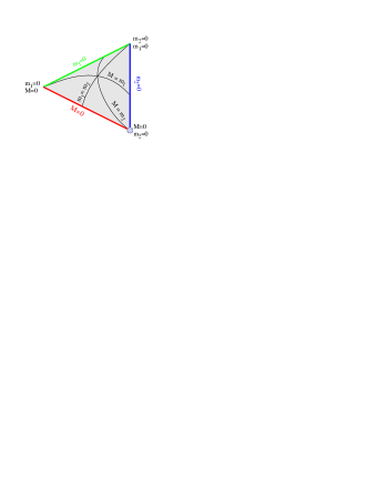
Figure 1: (Color online) Parameter space for the effective potential at $T=\mu=0$. The corner with $M=m_{2}=0$ indicates the QCD-like sector.

• $M=0$. Here, we have $m_{+}\neq m_{-}$ $(m_{2}\neq 0)$, and the gap equations become

  $$m_{1}\Bigl{(}\bar{\alpha}_{1}+\frac{1}{4\pi}\ln\frac{|m_{2}^{2}-m_{1}^{2}|}{\gamma}\Bigr{)}-\frac{m_{2}}{4\pi}\ln\Bigl{|}\frac{m_{1}-m_{2}}{m_{1}+m_{2}}\Bigr{|} =0\>,$$ (45)

  $$m_{2}\Bigl{(}\bar{\alpha}_{2}+\frac{1}{4\pi}\ln\frac{|m_{2}^{2}-m_{1}^{2}|}{\gamma}\Bigr{)}-\frac{m_{1}}{4\pi}\ln\Bigl{|}\frac{m_{1}-m_{2}}{m_{1}+m_{2}}\Bigr{|} =0\>.$$ (46)

• $m_{1}=0$. In this case, we have $m_{+}=-m_{-}=m_{2}$. The gap equations lead to

  $$m_{2}\Bigl{(}\bar{\alpha}_{2}+\frac{1}{4\pi}\ln\frac{|M^{2}-m_{2}^{2}|}{\gamma}\Bigr{)}-\frac{M}{4\pi}\ln\Bigl{|}\frac{M-m_{2}}{M+m_{2}}\Bigr{|} =0\>,$$ (47)

  $$M\Bigl{(}\bar{\beta}+\frac{1}{4\pi}\ln\frac{|M^{2}-m_{2}^{2}|}{\gamma}\Bigr{)}-\frac{m_{2}}{8\pi}\ln\Bigl{|}\frac{M-m_{2}}{M+m_{2}}\Bigr{|} =0\>.$$ (48)

• $m_{2}=0$ and we recover the symmetric-case results with $(m_{1}\neq 0,\,M\neq 0)$:

  $$m_{1}\Bigl{(}\bar{\alpha}_{1}+\frac{1}{4\pi}\ln\frac{|M^{2}-m_{1}^{2}|}{\gamma}\Bigr{)}\!-\!\frac{M}{4\pi}\ln\Bigl{|}\frac{M-m_{1}}{M+m_{1}}\Bigr{|}\!=0\>,$$ (49)

  $$M\Bigl{(}\bar{\beta}+\frac{1}{4\pi}\ln\frac{|M^{2}-m_{1}^{2}|}{\gamma}\Bigr{)}-\frac{m_{1}}{4\pi}\ln\Bigl{|}\frac{M-m_{1}}{M+m_{1}}\Bigr{|}\!=0\>.$$ (50)

Table 1: Position of the global minimum of the effective potential at $T=\mu=0$.

Parameters	masses	$V_{\mathrm{eff}}(m_{i},M)$
$\delta_{1}<\delta_{2}<0$ $(\Delta\delta>0)$	$M>m_{1}>m_{2}$	$V_{\mathrm{eff}}(0,0,M)$
$\delta_{2}<\delta_{1}<0$ $(\Delta\delta<0)$	$M>m_{2}>m_{1}$	$V_{\mathrm{eff}}(0,0,M)$
$\delta_{1}<0<\delta_{2}$ $(\Delta\delta>0)$	$m_{2}>M>m_{1}$	$V_{\mathrm{eff}}(0,m_{2},0)$
$0<\delta_{1}<\delta_{2}$ $(\Delta\delta>0)$	$m_{2}>m_{1}>M$	$V_{\mathrm{eff}}(0,m_{2},0)$
$0<\delta_{2}<\delta_{1}$ $(\Delta\delta<0)$	$m_{1}>m_{2}>M$	$V_{\mathrm{eff}}(m_{1},0,0)$
$\delta_{2}<0<\delta_{1}$ $(\Delta\delta<0)$	$m_{1}>M>m_{2}$	$V_{\mathrm{eff}}(m_{1},0,0)$

When only one mass ($m_{1}$, $m_{2}$, or $M$) is zero, (see appendix of Ref. symmetric ) the “global” minimum, along the side of the triangle, corresponds to one of its ends and which end exactly has the lower potential depends on the value of the parameters $\delta_{1}$, $\delta_{2}$, or $\Delta\delta$, respectively:

• If $\delta_{1}<0$, then $V_{\mathrm{eff}}(0,0,M)$ is the “global” minimum along the $m_{2}=0$ line, whereas if $\delta_{1}>0$ then the “global” minimum of the effective potential is $V_{\mathrm{eff}}(m_{1},0,0)$. The critical value $\delta_{1}=0$ corresponds to $M=m_{1}$.

• If $\delta_{2}<0$, then $V_{\mathrm{eff}}(0,0,M)$ is the “global” minimum along the $m_{1}=0$ line, whereas if $\delta_{2}>0$ then the “global” minimum of the effective potential is $V_{\mathrm{eff}}(0,m_{2},0)$. The critical value $\delta_{2}=0$ corresponds to $M=m_{2}$.

• If $\Delta\delta=\alpha_{1}-\alpha_{2}=\delta_{2}-\delta_{1}<0$, then $V_{\mathrm{eff}}(m_{1},0,0)$ is the “global” minimum along the $M=0$ line, whereas if $\Delta\delta>0$ then the “global” minimum of the effective potential is $V_{\mathrm{eff}}(0,m_{2},0)$. The critical value $\Delta\delta=0$ corresponds to $m_{1}=m_{2}$.

Following an approach similar to the one described in the appendix of Ref. symmetric , one can show that the effective potential in the case when all three masses $m_{i}$ and $M$ are nonzero, has a local minimum intermediate between the “corner” values. In conclusion, the global minimum of the effective potential at $T=\mu=0$ is always located at one of the corners of triangle depicted in Fig. 1. In Table 1 we show which corner corresponds to the global minimum of the effective, as a function of the relative values of the parameters $\delta_{1}$ and $\delta_{2}$.

V Phase Structure

We discuss now the effective potential (40) corresponding to the three possible vacuum phases identified in the previous section. We have:

• $m_{1}=m_{2}=0$. In this case our model reduces to the pure Cooper-pairing model ref:paper1 , with $M^{*2}=\Delta^{2}$ is the dynamically generated gap. Here, we choose $m_{10}=m_{20}=0$, $M_{0}^{2}=\Delta^{2}=\gamma$, and $\bar{\beta}=0$. Then, we can write

  $$V_{\mathrm{eff}}(m_{i},M)=\ m_{1}^{2}\bar{\alpha}_{1}+m_{2}^{2}\bar{\alpha}_{2}$$ (51)

  $$-\frac{1}{2}\int_{0}^{\infty}[\mathrm{d}k_{1}]\biggl{\{}k_{+}(m_{+})+k_{-}(m_{+})+k_{+}(m_{-})+k_{-}(m_{-})-4k_{1}-\frac{2(M^{2}\!+m_{1}^{2}\!+m_{2}^{2})}{\sqrt{k_{1}^{2}+\Delta^{2}}}$$

  $$+\!\frac{2}{\beta}\ln\bigl{[}1\!+\!e^{-\beta k_{+}(m_{+})}\bigr{]}\!+\!\frac{2}{\beta}\ln\bigl{[}1\!+\!e^{-\beta k_{-}(m_{+})}\bigr{]}\!+\!\frac{2}{\beta}\ln\bigl{[}1\!+\!e^{-\beta k_{+}(m_{-})}\bigr{]}\!+\!\frac{2}{\beta}\ln\bigl{[}1\!+\!e^{-\beta k_{-}(m_{-})}\bigr{]}\biggr{\}}\>.$$

  If we set $m_{1}=m_{2}=0$, then the chemical potential becomes irrelevant and can be transformed away. We obtain

  $$V_{\mathrm{eff}}(m_{i},M)=\ \frac{M^{2}}{4\pi}\Bigl{[}\ln\frac{M^{2}}{\Delta^{2}}-1\Bigr{]}-\frac{2}{\beta}\int_{0}^{\infty}[\mathrm{d}k_{1}]\Bigl{[}\ln\bigl{(}1\!+\!e^{-\beta E}\bigr{)}+\ln\bigl{(}1\!+\!e^{-\beta E}\bigr{)}\Bigr{]}\>,$$ (52)

  with $E=\sqrt{k_{1}^{2}+m_{2}^{2}}$.

  The effective potential for the Cooper pair sector at finite temperature is $\mu$ independent. The model has a second-order phase transition to the unbroken phase at a critical temperature ref:paper1 , $T_{\mathrm{c}}=(\Delta/\pi)\,e^{\gamma_{E}}$, where $\gamma_{E}=0.577\cdots$ is Euler’s constant.

• $M=m_{2}=0$. This is the Gross-Neveu sector ref:GN2 . Here, $m_{1}^{*2}=m_{\mathrm{F}}^{2}$ is the dynamically generated fermion mass. We choose $M_{0}=m_{20}=0$ and $m_{10}^{2}=m_{\mathrm{F}}^{2}=\gamma$. Furthermore, we have $g_{1\mathrm{R}}^{2}=\pi$ and $\bar{\alpha}_{1}=0$. Thus, we can write

  $$V_{\mathrm{eff}}(m_{i},M)=\ M^{2}\bar{\beta}+m_{2}^{2}\bar{\alpha}_{2}$$ (53)

  $$-\frac{1}{2}\int_{0}^{\infty}[\mathrm{d}k_{1}]\biggl{\{}k_{+}(m_{+})+k_{-}(m_{+})+k_{+}(m_{-})+k_{-}(m_{-})-4k_{1}-\frac{2(M^{2}\!+m_{1}^{2}\!+m_{2}^{2})}{\sqrt{k_{1}^{2}+m_{\mathrm{F}}^{2}}}$$

  $$+\!\frac{2}{\beta}\ln\bigl{[}1\!+\!e^{-\beta k_{+}(m_{+})}\bigr{]}\!+\!\frac{2}{\beta}\ln\bigl{[}1\!+\!e^{-\beta k_{-}(m_{+})}\bigr{]}\!+\!\frac{2}{\beta}\ln\bigl{[}1\!+\!e^{-\beta k_{+}(m_{-})}\bigr{]}\!+\!\frac{2}{\beta}\ln\bigl{[}1\!+\!e^{-\beta k_{-}(m_{-})}\bigr{]}\biggr{\}}\>.$$

  If we set $M=m_{2}=0$, then we obtain $m_{+}=m_{-}=m_{1}$, $k_{\pm}=E\pm\mu$ with $E=\sqrt{k_{1}^{2}+m_{1}^{2}}$, and the effective potential in the Gross-Neveu sector can be written as

  $$V_{\mathrm{eff}}(m_{i},M)=\ \frac{m_{1}^{2}}{4\pi}\Bigl{[}\ln\frac{m_{1}^{2}}{m_{\mathrm{F}}^{2}}-1\Bigr{]}-\frac{2}{\beta}\int_{0}^{\infty}[\mathrm{d}k_{1}]\Bigl{\{}\ln\bigl{[}1\!+\!e^{-\beta(E+\mu)}\bigr{]}+\ln\bigl{[}1\!+\!e^{-\beta(E-\mu)}\bigr{]}\Bigr{\}}\>.$$ (54)

  We note that the effective potential in the Gross-Neveu sector is similar to the effective potential in the Cooper pair sector, with $m_{\mathrm{F}}$ replacing $\Delta$, but depends on the chemical potential $\mu$ at $T\neq 0$.

  The Gross Neveu model has spontaneous symmetry breaking at zero chemical potential and zero temperature. At zero temperature, the model undergoes a first-order phase transition to the unbroken symmetry phase as we increase the chemical potential ref:GN2 ; ref:minakata . At zero chemical potential, the symmetry is restored through a second order phase transition at the critical temperature symmetric , $T_{\mathrm{c}}=(m_{\mathrm{F}}/\pi)\,\exp\bigl{[}\gamma_{E}-7\mu^{2}\zeta(3)/(4\pi^{2}T_{\mathrm{c}}^{2})\bigr{]}$. Thus, the phase diagram of the Gross-Neveu model has a tricritical point, with approximate values ref:GN2 $\mu_{c}/m_{F}=0.608,\,T_{c}/m_{F}=0.318$.

• $m_{1}=M=0$. Here, $m_{2}^{*2}=\delta m^{2}$ is the dynamically generated mass asymmetry. This case is identical with the Gross-Neveu sector case, with $m_{\mathrm{F}}$ being replaced by $\delta m$: We choose $m_{10}=M_{0}=0$, $m_{20}^{2}=\delta m^{2}=\gamma$, and $g_{1\mathrm{R}}^{2}=\pi$ (or $\bar{\alpha}_{2}=0$). The effective potential becomes

  $$V_{\mathrm{eff}}(m_{i},M)=\ M^{2}\bar{\beta}+m_{1}^{2}\bar{\alpha}_{1}$$ (55)

  $$-\frac{1}{2}\int_{0}^{\infty}[\mathrm{d}k_{1}]\biggl{\{}k_{+}(m_{+})+k_{-}(m_{+})+k_{+}(m_{-})+k_{-}(m_{-})-4k_{1}-\frac{2(M^{2}\!+m_{1}^{2}\!+m_{2}^{2})}{\sqrt{k_{1}^{2}+\delta m^{2}}}$$

  $$+\!\frac{2}{\beta}\ln\bigl{[}1\!+\!e^{-\beta k_{+}(m_{+})}\bigr{]}\!+\!\frac{2}{\beta}\ln\bigl{[}1\!+\!e^{-\beta k_{-}(m_{+})}\bigr{]}\!+\!\frac{2}{\beta}\ln\bigl{[}1\!+\!e^{-\beta k_{+}(m_{-})}\bigr{]}\!+\!\frac{2}{\beta}\ln\bigl{[}1\!+\!e^{-\beta k_{-}(m_{-})}\bigr{]}\biggr{\}}\>.$$

  When $m_{1}=M=0$, we obtain

  $$V_{\mathrm{eff}}(m_{i},M)=\ \frac{m_{2}^{2}}{4\pi}\Bigl{[}\ln\frac{m_{2}^{2}}{m_{\mathrm{F}}^{2}}-1\Bigr{]}-\frac{2}{\beta}\int_{0}^{\infty}[\mathrm{d}k_{1}]\Bigl{\{}\ln\bigl{[}1\!+\!e^{-\beta(E+\mu)}\bigr{]}+\ln\bigl{[}1\!+\!e^{-\beta(E-\mu)}\bigr{]}\Bigr{\}}\>,$$ (56)

  with $E=\sqrt{k_{1}^{2}+m_{2}^{2}}$.

VI Conclusions

In this paper we studied a generalization of a simple model with two spontaneously broken symmetry phases first discussed in Ref. symmetric . The model is studied in (1+1) dimensions within the leading order in large N approximation. We find that the phase diagram with two different masses is similar to the case when the masses are the same in that depending on the values of the two renormalized coupling constants one is always in one of three distinct phases.

A generalization of this model to higher dimensions including the case of spatially inhomogeneous order parameters is under development. We expect that the results found here in 1+1 for homogeneous order parameters will persist in mean field regardless of the number of dimensions. Thus, in order to obtain phase coexistence we will have to consider inhomogeneous condensates. For this type of condensates we expect a small coexistence region similar to the Larkin-Ovchinikov-Fulde-Ferrel state loff in ferromagnetic superconductors, while preserving the tricritical point.

After this work was completed, we became aware of a new study of the massive Gross-Neveu model using semi-classical methods in the large-N limit massive . These semi-classical methods display a kink-antikink crystal phase and it would be interesting to also perform such an analysis for the model of this paper. In 1+1 dimensions, semi-classical analyses such as those described by Dashen, Hasslacher and Neveu dhn often gave exact answers for the S-matrix (especially in exactly solvable models) and include more information than the straight forward study of the effective potential in the large-N approximation.

References

- (1) M. Alford, K. Rajagopal, and F. Wilczek, Phys. Lett. B 422, 247 (1998).
- (2) R. Rapp, T. Schäfer, E. V. Shuryak, and M. Velkovsky, Phys. Rev. Lett. 81, 53 (1998).
- (3) B. Kämpfer, Ann. Phys. (Leipzig) 9, 606 (2000).
- (4) N. D. Mathur et al., Nature 394, 39 (1998); S. S. Saxena et al., ibid. 406, 587 (2000).
- (5) J. A. Hertz, Phys. Rev. B 14, 1165 (1976); A. J. MILLIS, Phys. Rev. B 48, 7183 (1993).
- (6) A. Chodos, F. Cooper, W. Mao, H. Minakata, A. Singh, Phys. Rev. D 61, 045011 (2000).
- (7) N. I. Karchev, K. B. Blagoev, K. S. Bedell, and P. B. Littlewood, Phys. Rev. Lett. 86, 846 (2001); K. B. Blagoev, K. S. Bedell, and P. B. Littlewood ibid. 92, 199706 (2004).
- (8) A. I. Larkin and Yu. N. Ovchinnikov, Zh. Eksp. Teor. Fiz. 47, 1136 (1964) [Sov. Phys. JETP 20, 762 (1975)]; P. Fulde and R. A. Ferrell, Phys. Rev. 135, A550 (1964).
- (9) J. A. Bowers and K. Rajagopal, Phys. Rev. D 66, 065002 (2002); J. Kundu and K. Rajagopal, Phys. Rev. D 65, 094022 (2002).
- (10) D. J. Gross and A. Neveu, Phys. Rev. D10, 3235 (1974).
- (11) A. Chodos, H. Minakata, and F. Cooper, Phys. Lett. B 449, 260 (1999).
- (12) D. Bailin and A. Love, Phys. Rep. 107, 325 (1984); M. Iwasaki and T. Iwado, Phys. Lett. B 350, 163 (1995); M. Alford, K. Rajagopal and F. Wilczek, ibid. 422, 247 (1998).
- (13) M. Alford, K. Rajagopal and F. Wilczek, Nucl. Phys. A638, 515c (1998); Nucl. Phys. B537, 443 (1999); J. Berges and K. Rajagopal, ibid. B538, 215 (1999); T. Schäfer, Nucl. Phys. A642, 45 (1998); T. Schäfer and F. Wilczek, Phys. Rev. Lett. 82, 3956 (1999).
- (14) S. Coleman, Commun. Math. Phys. 31, 259 (1973); N. D. Mermin and H. Wagner, Phys. Rev. Lett. 17, 1133 (1966).
- (15) E. Witten, Nucl. Phys. B145, 110 (1978).
- (16) J. Hubbard, Phys. Rev. Lett. 3, 77 (1959); R. L. Stratonovich, Dokl. Akad. Nauk. SSSR 115, 1097 (1957) [Sov. Phys. Dokl. 2, 416 (1957)]; S. Coleman, Aspects of Symmetry (Cambridge University Press, Cambridge, England, 1985), p. 354.
- (17) If , then .
- (18) Note , , and .
- (19) , , , , , , , .
- (20) , , , , , , , , and , , , , , , , .
- (21) , for large .
- (22) Here, we have used , and .
- (23) For , we have .
- (24) U. Wolff, Phys. Lett. B 157, 303 (1985); L. Jacobs, Phys. Rev. D10, 3956 (1974); B. Harrington and A. Yildiz, Phys. Rev. D11, 779 (1975).
- (25) A. Chodos and H. Minakata, Phys. Lett. A 191, 39 (1994); Nucl. Phys. B490, 687 (1997).
- (26) O. Schnetz, M. Thies, and K. Urlichs, hep-th/0511206. See also M. Thies and K. Urlichs, Phys. Rev. D 67, 125015 (2003); M. Thies, ibid. 69, 067703 (2004); O. Schnetz, M. Thies, and K. Urlichs, Ann. Phys. 314, 425 (2004).
- (27) R.F. Dashen, B. Hasslacher, and A.Neveu, Phys. Rev. D 12, 2443 (1975).