ROM2F/2005/27

MS-TP-05-37

CERN-PH-TH/2005-268

FTUAM-05-20

IFT UAM-CSIC/05-55

DESY 05-259

December 2005

A precise determination of $B_{K}$ in quenched QCD

P. Dimopoulos^a, J. Heitger^b, F. Palombi^c, C. Pena^d, S. Sint^e and A. Vladikas^a

^a INFN, Sezione di Roma II

and Dipartimento di Fisica, Università di Roma “Tor Vergata”

Via della Ricerca Scientifica 1, I-00133 Rome, Italy

^b Westfälische Wilhelms-Universität Münster, Institut für Theoretische Physik

Wilhelm-Klemm-Strasse 9, D-48149 Münster, Germany

^c DESY, Theory Group, Notkestrasse 85, D-22603 Hamburg, Germany

^d CERN, Physics Department, TH Division, CH-1211 Geneva 23, Switzerland

^e Departamento de Física Teórica C-XI and

Instituto de Física Teórica C-XVI,

Universidad Autónoma de Madrid, Cantoblanco E-28049 Madrid, Spain

 Abstract The $B_{K}$ parameter is computed in quenched lattice QCD with Wilson twisted mass fermions. Two variants of tmQCD are used; in both of them the relevant $\Delta S=2$ four-fermion operator is renormalised multiplicatively. The renormalisation adopted is non-perturbative, with a Schrödinger functional renormalisation condition. Renormalisation group running is also non-perturbative, up to very high energy scales. In one of the two tmQCD frameworks the computations have been performed at the physical $K$-meson mass, thus eliminating the need of mass extrapolations. Simulations have been performed at several lattice spacings and the continuum limit was reached by combining results from both tmQCD regularisations. Finite volume effects have been partially checked and turned out to be small. Exploratory studies have also been performed with non-degenerate valence flavours. The final result for the RGI bag parameter, with all sources of uncertainty (except quenching) under control, is $\hat{B}_{K}=0.789\pm 0.046$.  

1 Introduction

Indirect CP-violation in $K\rightarrow\pi\pi$ decays is expressed in terms of the $\epsilon$-parameter. Its known experimental value, combined with theoretical input from neutral $K$-meson oscillations, defines a hyperbola in the complex plane of the unitarity triangle (for a review see ref. [1]). The theoretical prediction of the oscillation amplitude is obtained in an operator product expansion framework, as the product of a single Wilson coefficient (known to NLO in perturbation theory [2, 3]) and the matrix element $\langle\bar{K}^{0}|O^{\Delta S=2}|K^{0}\rangle$ of a dimension-6, $\Delta S=2$ operator

$$O^{\Delta S=2} \equiv [\bar{s}\gamma_{\mu}(1-\gamma_{5})d]\,\,[\bar{s}\gamma_{\mu}(1-\gamma_{5})d]$$ (1.1)

$$= O_{\rm VV+AA}-O_{\rm VA+AV}\,.$$

Here $s$ and $d$ are strange and down quark fields. Within the square brackets spin and colour indices are saturated. In obvious notation, the operators $O_{\rm VV+AA}$ and $O_{\rm VA+AV}$ are the parity-even and -odd parts of $O^{\Delta S=2}$. For historical and technical reasons, this matrix element is usually normalised by its value in the vacuum saturation approximation (VSA). It is thus expressed in terms of the $B_{K}$ parameter:

$$B_{K}\equiv\dfrac{\langle\bar{K}^{0}|O_{\rm VV+AA}|K^{0}\rangle}{\langle\bar{K}^{0}|O_{\rm VV+AA}|K^{0}\rangle_{VSA}}=\dfrac{\langle\bar{K}^{0}|O_{\rm VV+AA}|K^{0}\rangle}{\dfrac{8}{3}F_{K}^{2}m_{K}^{2}}\,,$$ (1.2)

with $m_{K}$ the $K$-meson mass and $F_{K}$ its decay constant. The above expression involves the matrix element of the parity-even operator $O_{\rm VV+AA}$ only. The parity-odd matrix element $\langle\bar{K}^{0}|O_{\rm VA+AV}|K^{0}\rangle_{VSA}$ vanishes identically in QCD.

$B_{K}$ is an intrinsically non-perturbative quantity, which can be computed in the lattice regularisation of QCD. The results of the various recent $B_{K}$ measurements have been summarised in ref. [4] (see also references in this review). Besides quenching, which is a still uncontrolled source of systematic error, the most important source of uncertainty in these computations arises from the operator renormalisation. In schemes which respect chiral symmetry, the operator $O_{\rm VV+AA}$ is multiplicatively renormalisable. Thus, the corresponding physical matrix element can in principle be accurately obtained by a series of non-perturbative (lattice) measurements of the bare matrix element and the operator renormalisation constant, at several values of the lattice spacing, followed by a continuum limit extrapolation. This is the case of Ginsparg-Wilson fermions, where chiral symmetry-breaking effects are negligible. With Wilson fermions, the breaking of chiral symmetry induces mixing with four other dimension-6 operators [5, 6, 7, 8, 9] in the parity-even sector:

$$(O_{\rm R})_{\rm VV+AA}=Z_{\rm VV+AA}(g_{0},a\mu)\Big{[}O_{\rm VV+AA}(g_{0})+\sum_{i=1}^{4}\Delta_{i}(g_{0})O_{i}(g_{0})\Big{]}\,.$$ (1.3)

The operators $O_{i}(g_{0})$ belong to different chiral representations than $O_{\rm VV+AA}$. The mixing coefficients $\Delta_{i}(g_{0})$ are finite functions of the bare coupling, while the renormalisation constant $Z_{\rm VV+AA}(g_{0},a\mu)$ diverges logarithmically. This mixing pattern is the reason behind the relatively poor precision of $B_{K}$, measured with Wilson fermions.

Two proposals have attempted to resolve this issue. They are both based on the observation [7, 9] that, even in the absence of chiral symmetry, the parity-odd operator $O_{\rm VA+AV}$ is protected from mixing with others, by discrete symmetries:

$$(O_{\rm R})_{\rm VA+AV}=Z_{\rm VA+AV}(g_{0},a\mu)O_{\rm VA+AV}(g_{0})\,.$$ (1.4)

The first proposal [10] consists in obtaining the physical $K^{0}-\bar{K}^{0}$ matrix element of $O_{\rm VV+AA}$ from a correlation function of the renormalised operator $O_{\rm VA+AV}$, through axial Ward identities. The method has been put to test in ref. [11]. The $B_{K}$ estimate of this method turned out to be compatible with the result of the standard computation (with operator subtractions). Unfortunately, the correlation function of $O_{\rm VA+AV}$, being the product of four composite operators, turned out to be noisy and the error was as large as the one of the standard computation. Thus, this method is successful in eliminating an important source of systematic errors (operator subtraction) at the cost of increased statistical fluctuations.

In this work we implement the second proposal [12], which is based on the addition of a so-called “twisted mass term” to the Wilson fermion action. This entails loss of parity and partial loss of flavour symmetry at finite lattice spacing, recovered in the continuum limit. On the other hand, some renormalisation properties are greatly ameliorated in the twisted mass QCD (tmQCD) formalism. The relevant case for us is the renormalised $\langle\bar{K}^{0}|O_{\rm VV+AA}|K^{0}\rangle$ matrix element, which in the tmQCD formalism may be expressed in terms of the parity-odd operator $O_{\rm VA+AV}$. The tmQCD action differs from the standard one by an additional soft term, which does not modify renormalisation properties in mass independent renormalisation schemes. In particular, the operator $O_{\rm VA+AV}$ remains multiplicatively renormalisable, with the same renormalisation constant and running as with Wilson fermions. Thus finite subtractions are avoided in the tmQCD determination of $B_{K}$.

With respect to previous studies, we have introduced several new features:

• The bare matrix elements have been obtained in two distinct lattice tmQCD formulations. In the first formulation, the down quark is twisted, with a twist angle $\alpha=\pi/2$, while the strange quark is a standard (untwisted) Wilson fermion. In the second formulation we have a twisted flavour doublet of down and strange flavours, with twist angle $\alpha=\pi/4$. Having two independent $B_{K}$ estimates allows a better control of the continuum limit extrapolations. We have implemented Schrödinger functional (SF) boundary conditions for these computations.

• Quenched simulations with standard Wilson fermions are carried out at heavier quark masses, due to the presence of exceptional configurations. Since our tmQCD variant with $\alpha=\pi/4$ is free of exceptional configurations, $B_{K}$ can be computed at the physical $K$-meson mass value. Thus the error due to extrapolations from higher masses is eliminated.

• In ref. [13] the operator $O_{\rm VA+AV}$ has been renormalised non-perturbatively in several SF renormalisation schemes and its Renormalisation Group (RG) running has been computed non-perturbatively from low energies up to scales of several tens of GeV. We have used these results in order to obtain the Renormalisation Group Invariant (RGI) counterpart of $B_{K}$. Our result is essentially free of any uncertainty due to Perturbation Theory (PT).

• Although our main results have been obtained with degenerate down and strange quarks, we have also performed some exploratory studies with non-degenerate flavours. Also, some simulations have been performed in order to probe finite volume effects.

Our result confirms earlier ones, obtained from other lattice regularisations (domain wall, overlap, staggered) albeit with a major control of the various sources of error. An interesting discrepancy with the result of the most recent detailed study of $B_{K}$ with Wilson fermions (see ref. [11]) is also resolved.

The paper is organized as follows: In sect. 2 we review the tmQCD basics, emphasising the cases of interest. We show how, by choosing either a twist angle $\alpha=\pi/2$ or $\alpha=\pi/4$, we can map the operator $O_{\rm VV+AA}$ onto $O_{\rm VA+AV}$, thus achieving multiplicative renormalisation without subtractions. In sect. 3 we review how four-fermion operator matrix elements can be obtained from SF correlation functions. In sects. 4 and 5 we present our raw results for tmQCD with $\alpha=\pi/2$ and $\alpha=\pi/4$ respectively. In sect. 6 we compute the RGI-$B_{K}$, extrapolated to the continuum limit. Several more technical aspects are discussed in the appendices.

Preliminary results of our work have appeared in refs. [14, 15]. Based on a similar approach, the $\bar{B}^{0}-B^{0}$ matrix element, with a static bottom flavour, is currently under study [16, 17].

2 Twisted mass QCD and weak matrix elements

Twisted mass QCD has been designed to eliminate exceptional configurations in (partially) quenched lattice simulations with light Wilson quarks [12]. In its original formulation, it describes a mass-degenerate isospin doublet $\psi$ of Wilson quarks for which, besides the standard mass term, a so-called twisted mass term $i\mu_{\rm q}\bar{\psi}\gamma_{5}\tau^{3}\psi$ is introduced. The properties of tmQCD have been studied in detail in  [12], where, in particular, its equivalence to standard two-flavour QCD has been established. We discuss here two extensions of this framework, which are suited to the extraction of $B_{K}$.

2.1 Twisted mass QCD with twist angle $\pi/2$

The first variant has already been mentioned in ref. [12], and corresponds to a Euclidean continuum action of the form

$$S_{F}=\int{\rm d}^{4}x\,\,[\bar{\psi}(x)({\kern 2.5pt/\kern-6.99997ptD}+m_{l}+i\mu_{l}\gamma_{5}\tau^{3})\psi(x)+\bar{s}(x)({\kern 2.5pt/\kern-6.99997ptD}+m_{s})s(x)]\ .$$ (2.5)

Here, the two light flavours form an isospin doublet $\psi^{T}=(u,d)$, $\tau^{3}$ is a Pauli matrix and $\mu_{l}$ and $m_{l}$ are the twisted and standard quark mass parameters. For the light quark sector the physical quark mass is given

$$M_{l}=\sqrt{m_{l}^{2}+\mu_{l}^{2}}\ ,$$ (2.6)

and the twist angle is defined by

$$\tan\alpha=\dfrac{\mu_{l}}{m_{l}}\ .$$ (2.7)

The considerable advantages of the choice $\alpha=\pi/2$, for which $m_{l}=0$ and $M_{l}=\mu_{l}$, will be discussed below. We will refer to this case as “fully twisted”, since the physical quark mass $M_{l}$ is determined by the twisted mass parameter alone.

The equivalence of this theory to standard QCD, established in  [12], is based on axial transformations of the quark fields and corresponding spurionic transformations of the mass parameters. Let us relabel the fields and masses of the above theory by $\psi^{(\alpha)},m_{l}^{(\alpha)}$ and $\mu_{l}^{(\alpha)}$. The corresponding quantities in standard QCD (which is tmQCD at $\alpha=0$) are given by $\psi^{(0)},m_{l}^{(0)}$ and $\mu_{l}^{(0)}=0$. The two theories are then related by the axial field transformations

$$\psi^{(\alpha)}\to\psi^{(0)}=R(\alpha)\psi^{(\alpha)},\qquad\overline{\psi}^{(\alpha)}\to\overline{\psi}^{(0)}=\overline{\psi}^{(\alpha)}R(\alpha)\ ,$$ (2.8)

and the transformation of the mass parameter

$$m_{l}^{(0)}=m_{l}^{(\alpha)}\cos(\alpha)+\mu_{l}^{(\alpha)}\sin(\alpha)\ ,$$ (2.9)

where

$$R(\alpha)=\exp\left\{\hbox{$i\over 2$}\gamma_{5}\alpha\tau^{3}\right\}\ .$$ (2.10)

In tmQCD we denote Euclidean correlation functions by

$$\left\langle O[\psi,\overline{\psi}]\right\rangle_{(\alpha)}={\cal Z}^{-1}\int_{\rm fields}O[\psi,\overline{\psi}]{\rm e}^{-S},$$ (2.11)

where $O[\psi,\overline{\psi}]$ denotes some multilocal gauge invariant field. The fermionic part of the action is given in (2.5). The relation between standard QCD and tmQCD correlation functions, are then expressed as

$$\left\langle O\left[\psi,\overline{\psi}\right]\right\rangle_{(\alpha)} = \left\langle O\left[R(-\alpha)\psi,\overline{\psi}R(-\alpha)\right]\right\rangle_{(0)},$$ (2.12)

$$\left\langle O\left[\psi,\overline{\psi}\right]\right\rangle_{(0)} = \left\langle O\left[R(\alpha)\psi,\overline{\psi}R(\alpha)\right]\right\rangle_{(\alpha)}.$$ (2.13)

Hence, a given correlation function in tmQCD with twist angle $\alpha$ is interpreted as the linear combination on the r.h.s. of Eq. (2.12). If instead we are given a standard QCD correlation function, then Eq. (2.13) tells us how it is represented in tmQCD at twist angle $\alpha$.

In the formal continuum framework, all these relations between tmQCD and standard QCD quantities are readily obtained from the chiral transformations (2.8). Their extension to the lattice regularised theory with Wilson fermions, which is the lattice regularisation of choice in the present work, is more intricate. As shown in [12], the same relations are realised between the renormalised quantum field theories, provided the renormalisation procedure is set up with some care. Moreover, the definitions (2.6) and (2.7) are understood to hold for suitably renormalised masses $M_{{\rm R},l}$, $m_{{\rm R},l}$ and $\mu_{{\rm R},l}$, such that the twist angle $\alpha$ is free of renormalisation.

2.1.1 Relations between composite fields

The axial transformations (2.8) induce a mapping between composite fields. For the quark bilinear operators

$$S_{ij}=\bar{\psi}_{i}\psi_{j},\quad P_{ij}=\bar{\psi}_{i}\gamma_{5}\psi_{j},\quad A_{\mu,ij}=\bar{\psi}_{i}\gamma_{\mu}\gamma_{5}\psi_{j},\quad V_{\mu,ij}=\bar{\psi}_{i}\gamma_{\mu}\psi_{j},$$ (2.14)

we have

$$S_{sd}^{(0)} =\cos\left(\tfrac{\alpha}{2}\right)S_{sd}^{(\alpha)}\hskip 4.8pt-i\sin\left(\tfrac{\alpha}{2}\right)P_{sd}^{(\alpha)},$$ (2.15)

$$P_{sd}^{(0)} =\cos\left(\tfrac{\alpha}{2}\right)P_{sd}^{(\alpha)}\hskip 3.2pt-i\sin\left(\tfrac{\alpha}{2}\right)S_{sd}^{(\alpha)},$$ (2.16)

$$A_{\mu,sd}^{(0)} =\cos\left(\tfrac{\alpha}{2}\right)A_{\mu,sd}^{(\alpha)}-i\sin\left(\tfrac{\alpha}{2}\right)V_{\mu,sd}^{(\alpha)},$$ (2.17)

$$V_{\mu,sd}^{(0)} =\cos\left(\tfrac{\alpha}{2}\right)V_{\mu,sd}^{(\alpha)}\hskip 1.8pt-i\sin\left(\tfrac{\alpha}{2}\right)A_{\mu,sd}^{(\alpha)}\ .$$ (2.18)

For the four-quark operators under consideration we have:

$$O^{(0)}_{\rm VV+AA} = \cos\left(\alpha\right)O^{(\alpha)}_{\rm VV+AA}-i\sin\left(\alpha\right)O^{(\alpha)}_{\rm VA+AV}\ ,$$ (2.19)

$$O^{(0)}_{\rm VA+AV} = \cos\left(\alpha\right)O^{(\alpha)}_{\rm VA+AV}-i\sin\left(\alpha\right)O^{(\alpha)}_{\rm VV+AA}.$$ (2.20)

The case of interest is $\alpha=\pi/2$, for which we have

$$A^{(0)}_{\mu,sd} =\dfrac{\sqrt{2}}{2}[A_{\mu,sd}^{(\pi/2)}-iV_{\mu,sd}^{(\pi/2)}]\ ,$$ (2.21)

$$O^{(0)}_{\rm VV+AA} =-iO^{(\pi/2)}_{\rm VA+AV}, O^{(0)}_{\rm VA+AV}=-iO^{(\pi/2)}_{\rm VV+AA}\ .$$ (2.22)

The above formal expressions imply the following relation between renormalised operator matrix elements:

$$\langle K^{0}|\,\,(O_{\rm R})^{(0)}_{\rm VV+AA}\,\,|\bar{K}^{0}\rangle=-i\langle K^{0}|\,\,(O_{\rm R})_{\rm VA+AV}^{(\pi/2)}\,\,|\bar{K}^{0}\rangle\,.$$ (2.23)

The advantage of computing $B_{K}$ from the matrix element on the rhs (i.e. by performing a tmQCD computation), is that $O_{\rm VA+AV}$ is multiplicatively renormalisable, whereas the matrix element on the lhs involves $O_{\rm VV+AA}$, which requires additive renormalisation.

2.2 Twisted mass QCD with twist angle $\pi/4$

We also implemented a second variant of tmQCD, in which the down and strange quarks are grouped into a flavour doublet $\psi^{T}=(s,d)$:

$$S_{F}=\int{\rm d}^{4}x\,\,\left[\bar{\psi}(x)({\kern 2.5pt/\kern-6.99997ptD}+m_{l}+i\gamma_{5}\tau^{3}\mu_{l})\psi(x)+\bar{u}(x)({\kern 2.5pt/\kern-6.99997ptD}+m_{u})u(x)\right]\ .$$ (2.24)

This formulation of the theory is suitable for $B_{K}$ studies with degenerate light and strange valence flavours. In the quenched approximation, the first term alone is adequate for $B_{K}$ simulations, since only strange and down valence quarks are involved. In this approximation it is straightforward to also accommodate non-degenerate valence flavours, by introducing diagonal $2\times 2$ mass matrices in place of $m_{l}$ and $\mu_{l}$ (see ref. [18]) for details).

The general relationships of subsect. 2.1, defining total quark mass, twist angle and chiral rotations between fermion fields, mass parameters and correlation functions, hold also in this case. Once more, they are valid both formally and between renormalised quantities.

2.2.1 Relations between composite fields

In the present tmQCD formulation, the chiral rotations between composite fields become

$$S_{sd}^{(0)} = S_{sd}^{(\alpha)},$$ (2.25)

$$P_{sd}^{(0)} = P_{sd}^{(\alpha)},$$ (2.26)

$$A_{\mu,sd}^{(0)} = \cos\left(\alpha\right)A_{\mu,sd}^{(\alpha)}-i\sin\left(\alpha\right)V_{\mu,sd}^{(\alpha)},$$ (2.27)

$$V_{\mu,sd}^{(0)} = \cos\left(\alpha\right)V_{\mu,sd}^{(\alpha)}-i\sin\left(\alpha\right)A_{\mu,sd}^{(\alpha)}.$$ (2.28)

For the four-quark operators of interest we have:

$$O^{(0)}_{\rm VV+AA} = \cos\left(2\alpha\right)O^{(\alpha)}_{\rm VV+AA}-i\sin\left(2\alpha\right)O^{(\alpha)}_{\rm VA+AV},$$ (2.29)

$$O^{(0)}_{\rm VA+AV} = \cos\left(2\alpha\right)O^{(\alpha)}_{\rm VA+AV}-i\sin\left(2\alpha\right)O^{(\alpha)}_{\rm VV+AA}.$$ (2.30)

At $\alpha=\pi/4$ we have

$$A^{(0)}_{\mu,sd} =\dfrac{\sqrt{2}}{2}[A_{\mu,sd}^{(\pi/4)}-iV_{\mu,sd}^{(\pi/4)}],$$ (2.31)

$$O^{(0)}_{\rm VV+AA} =-iO^{(\pi/4)}_{\rm VA+AV}\ , O^{(0)}_{\rm VA+AV}=-iO^{(\pi/4)}_{\rm VV+AA}\ .$$ (2.32)

The formal above expressions imply for the renormalised WME of interest

$$\langle K^{0}|\,\,(O_{R})_{\rm VV+AA}^{(0)}\,\,|\bar{K}^{0}\rangle=-i\langle K^{0}|\,\,(O_{R})_{\rm VA+AV}^{(\pi/4)}\,\,|\bar{K}^{0}\rangle\ .$$ (2.33)

Here, as in the $\pi/2$ case, we see that the QCD four-fermion WME of interest is mapped onto a tmQCD WME which involves the multiplicatively renormalisable four-fermion operator $O_{\rm VA+AV}$. So from the renormalisation point of view, the $\pi/4$ version is equally advantageous.

2.3 Flavour symmetry, strangeness and mass degeneracy

The two tmQCD formalisms exposed above have distinct characteristics, which merit some discussion. The $\pi/2$ case refers to a light flavour doublet, while the strange quark is regularised in the standard way. Thus simulations may be naturally performed with non-degenerate down and strange flavours. In particular, simulations may get close to the physical situation, since the twisted light quarks are protected from exceptional configurations, whereas the non-twisted strange quark is heavy enough to remain unaffected by this problem.

At this point we note that most quenched computations of $B_{K}$ have remained with mass degenerate down and strange quarks, simply because quenched chiral perturbation theory indicates the appearance of potentially dangerous quenched chiral logs as soon as one departs from this situation [19, 20, 21, 22]. In this unphysical situation, the problem of exceptional configurations re-appears for the strange quark. Thus one is forced to stay with fairly massive pseudoscalar mesons of about $600~{}{\rm MeV}$, where the problem of exceptional configurations is believed to be absent, at least with a non-perturbatively ${\rm O}(a)$ improved action [23]. In quenched computations with degenerate strange and down masses, one must therefore compute $B_{K}$ with the $K-$meson tuned to several values above its physical mass and then extrapolate to the physical point.

While in the $\alpha=\pi/2$ scenario some tuning of the quark mass parameters is necessary to achieve mass degeneracy between the down and the strange quark (see below), this unphysical situation is naturally obtained in the $\pi/4$ case where down and strange quarks form a flavour doublet. The problem of exceptional configurations is now absent. This enables the computation of $B_{K}$ with degenerate valence quarks tuned so as to have the $K$-meson at its physical mass value, avoiding extrapolations from heavier masses.

More generally, it must be realised that partial loss of flavour symmetry at finite lattice spacing is the price one has to pay for the attractive features of tmQCD. Surprisingly large flavour breaking effects have been observed with maximally twisted Wilson quarks at $c_{\rm sw}=0$ in refs. [24, 25]. We have also looked at flavour breaking effects and found that these are reasonably small and rapidly decreasing towards the continuum limit (cf. sect. 4). The question whether these different findings are due to differences of the lattice action, parameters or the choice of observables will be the subject of further study.

2.4 Improvement considerations

Lattice quantities are computed at several fixed UV cutoffs and, after they are renormalised, they are extrapolated to the continuum limit. Symanzik improvement, if applied, ensures a better control of the extrapolating procedure. It involves adding ${\rm O}(a)$ counterterms both in the lattice action and the operators. In this work we will be using the Clover improved action [26] and improved currents (in the spirit of ref. [27, 28]).

Use of the Clover improved action implies that our meson mass estimates are subject to finite spacing effects which are $O(a^{2})$. In order to remove ${\rm O}(a)$ cutoff effects from $B_{K}$, we would also need to improve the relevant matrix elements of the four-fermion operator and the axial current in the tmQCD regularisation. The improvement pattern of dimension-3 quark bilinear operators in the quenched approximation is given in Appendix B. For tmQCD with untwisted (strange) and twisted (down) quarks, these results give for the currents

$$(A_{\rm R})_{\mu,sd} = Z_{\rm A}[1+\hbox{$1\over 2$}b_{\rm\scriptscriptstyle A}am_{q,s}][A_{\mu,sd}+c_{\rm A}a\tilde{\partial}_{\mu}P_{sd}-i\hbox{$1\over 2$}a\mu_{l}\tilde{b}_{\rm\scriptscriptstyle A}V_{\mu,sd}]\,,$$ (2.34)

$$(V_{\rm R})_{\mu,sd} = Z_{\rm V}[1+\hbox{$1\over 2$}b_{\rm\scriptscriptstyle V}am_{q,s}][V_{\mu,sd}+c_{\rm V}a\tilde{\partial}_{\nu}T_{\mu\nu,sd}-i\hbox{$1\over 2$}a\mu_{l}\tilde{b}_{\rm\scriptscriptstyle V}A_{\mu,sd}]\,,$$ (2.35)

where the subscript ${\rm R}$ refers to renormalised quantities and $\tilde{\partial}$ stands for the symmetric lattice derivative. These renormalised currents combine as in Eq. (2.21) to give the improved axial current in the $\alpha=\pi/2$ case. For tmQCD with the down and strange quarks in the same (twisted) doublet, the results of [29] can be directly taken over (with the up quark replaced by the strange one). We thus have

$$(A_{\rm R})_{\mu,sd} = Z_{\rm A}[1+b_{\rm\scriptscriptstyle A}am_{\rm q}][A_{\mu,sd}+c_{\rm A}a\tilde{\partial}_{\mu}P_{sd}-ia\mu_{l}\tilde{b}_{\rm\scriptscriptstyle A}V_{\mu,sd}]\,,$$ (2.36)

$$(V_{\rm R})_{\mu,sd} = Z_{\rm V}[1+b_{\rm\scriptscriptstyle V}am_{\rm q}][V_{\mu,sd}+c_{\rm V}a\tilde{\partial}_{\nu}T_{\mu\nu,sd}-ia\mu_{l}\tilde{b}_{\rm\scriptscriptstyle V}A_{\mu,sd}]\,.$$ (2.37)

These renormalised currents combine as in Eq. (2.31) to give the improved axial current in the $\alpha=\pi/4$ case. The renormalisation constants and improvement coefficients used here may be found in Appendix A.

The improvement of four-fermion operators is a far more difficult procedure. Though feasible in principle, it is rendered impractical by the proliferation of counterterms. We will hence not proceed in this direction.

Following these considerations, we have always used the Clover action in our simulations. The four-fermion operator is left unimproved. The implications of current improvement to the O($a$) effects of $B_{K}$ require further discussion. We will repeatedly revert to this issue at later stages.

2.5 Tuning of quark masses

With the continuum actions (2.5) and (2.24) the twist angle is directly determined by the ratio of the mass parameters $m_{l}$, $\mu_{l}$ in the action. This is no longer the case once tmQCD has been regularised with Wilson type quarks. Rather, the tuning of the twist angle $\alpha$ to the preferred values $\pi/2$ and $\pi/4$ requires the implementation of Eq. (2.7) for renormalised mass parameters. We discuss this issue in some detail.

We denote the subtracted bare quark mass for Wilson fermions by $am_{\rm q}=1/(2\kappa)-1/(2\kappa_{cr})$, $\kappa$ being the hopping parameter. Whenever we need to identify the quark flavour $f$, we will denote the corresponding quantities by $am_{{\rm q},f}$ and $\kappa_{f}$. For the untwisted strange quark in the $\pi/2$ formulation, the renormalised quenched quark mass is given by

$$m_{{\rm R},s} = Z_{\rm m}[m_{{\rm q},s}(1+b_{\rm m}am_{{\rm q},s})]\,,$$ (2.38)

while the light quark masses renormalise as follows:

$$m_{{\rm R},l} = Z_{\rm m}[m_{{\rm q},l}(1+b_{\rm m}am_{{\rm q},l})+\tilde{b}_{\rm m}a\mu_{l}^{2}]\,,$$

$$\mu_{{\rm R},l} = Z_{\mu}\mu_{l}(1+b_{\mu}am_{{\rm q},l})\,.$$ (2.39)

The above expressions are valid up to $O(a^{2})$ corrections. For the strange flavour, Eq. (2.38) is the standard relationship between renormalised quark mass and $\kappa_{s}$. For the light sector, fixing the twist angle to $\pi/2+O(a^{2})$ amounts to setting $m_{{\rm R},l}=0$ with $\mu_{{\rm R},l}$ positive. In other words, once a value $a\mu_{l}$ is chosen, we tune $\kappa_{l}$ so as to satisfy

$$am_{{\rm q},l}=-\tilde{b}_{\rm m}(a\mu_{l})^{2}\,.$$ (2.40)

The $\pi/4$ case is somewhat less trivial. In order to ensure that the twist angle acquires this value to $O(a^{2})$, we must impose $\mu_{\rm R}=m_{\rm R}$ to this order in the cutoff effects (flavour indices are suppressed, as the formalism applies to degenerate down and strange quarks). In terms of eqs. (2.39) this means

$$am_{\rm q}=\dfrac{1}{ZZ_{\rm A}}a\mu_{\rm q}\big{\{}1+\big{[}\dfrac{1}{ZZ_{\rm A}}(b_{\mu}-b_{\rm m})-ZZ_{\rm A}\tilde{b}_{\rm m}\big{]}a\mu_{q}\big{\}}\,,$$ (2.41)

with $Z\equiv Z_{\rm m}/(Z_{\mu}Z_{\rm A})$. For a given choice of $a\mu_{\rm q}$ and $\kappa_{cr}$, $\kappa$ is tuned so that $am_{\rm q}$ satisfies the above relation.

In Appendix A we collect the known results for the renormalisation constants and improvement coefficients required above.

3 SF Correlation functions at large time separations

We now derive explicit expressions for the representation of Schrödinger functional correlation functions in terms of intermediate physical states. For quark bilinear dimension-3 operators (e.g. the pseudoscalar density, or the axial vector current) this has been discussed in ref. [31]. Here we recapitulate the derivation and generalise it, in a straightforward manner, to the four-quark dimension-6 operator of interest. We then discuss how this formalism extends to the case of tmQCD.

3.1 Quantum mechanical representation of the Schrödinger functional

The QCD Schrödinger functional is defined as the QCD partition function in Euclidean space-time, with quark and gluon fields obeying periodic boundary conditions in space (with period $L$) and Dirichlet boundary conditions in time at the hypersurfaces $x_{0}=0$ and $x_{0}=T$. We assume homogeneous boundary conditions, i.e. the spatial components of the gauge potentials and the Dirichlet components of the quark and anti-quark fields are taken to vanish at the two time boundaries. The Schrödinger functional can then be written as [32, 33]

$${{\cal Z}}=\langle{\rm i_{0}}|{\rm e}^{-T\mathbb{H}}\,\mathbb{P}\,|{\rm i_{0}}\rangle\,,$$ (3.42)

where $|{\rm i}_{0}\rangle$ is a state which is implicitly defined by the Dirichlet conditions, and carries the quantum numbers of the vacuum state. The presence of $\,\mathbb{P}\,$ implies a projection onto the subspace of gauge invariant states, and $\mathbb{H}$ denotes the Hamilton operator of QCD formulated on a torus of volume $L^{3}$. It is the existence of the Hamiltonian operator which allows for the definition of a time-zero quantum mechanical Hilbert space and the corresponding operator representation of Euclidean correlation functions. On the lattice, $a\,\mathbb{H}$ is defined as the negative logarithm of the transfer matrix and it is Hermitian provided the transfer matrix itself is Hermitian and positive. This is indeed the case with the standard Wilson gauge action and unimproved Wilson quarks with both standard and twisted mass terms [34, 29]. In principle, this property is lost in the presence of O($a$) improvement terms in the action. However, the ensuing unitarity violations are usually considered harmless since they occur close to the cutoff scale and thus do not affect the physics at low energies [35].

The quantum mechanical representation of correlation functions then proceeds via the introduction of a set of (gauge invariant) eigenstates of $\mathbb{H}$,

$$|n,q\rangle\,,\quad n=0,1,\ldots\;,$$ (3.43)

$$\mathbb{H}\,|n,q\rangle=E^{(q)}_{n}|n,q\rangle\,,$$ (3.44)

with normalisation $\langle n^{\prime},q^{\prime}|n,q\rangle=\delta_{n,n^{\prime}}\,\delta_{q,q^{\prime}}$. Here, $q$ is a multi-index comprising all quantum numbers corresponding to the exact lattice symmetries, and $n$ enumerates the energy levels in the channel specified by $q$. We do not indicate the momentum of the states $|n,q\rangle$, since we will always be working with correlation functions that project states with vanishing (spatial) momentum.

Note that in general the set of conserved lattice quantum numbers $q$ is smaller than in the continuum, due to the explicit breaking of symmetries by the lattice regularisation. Standard Wilson quarks have the nice property to conserve an exact SU($N_{\rm f}$) flavour symmetry, besides parity and charge conjugation symmetries. The only difference to the continuum classification of particle states then consists in the breaking of rotational symmetries by the lattice regularisation, which implies that angular momentum is not a good quantum number in general. However, this mainly affects higher spin states, and is irrelevant for the pseudoscalar meson states at hand. In the following we first give an account of this continuum like situation with standard Wilson quarks before turning to the more complicated case of tmQCD.

3.2 Specific cases of SF correlation functions

For the calculation of $B_{K}$, we are interested in specific correlation functions of gauge invariant dimension-3 quark bilinear operators $X$ (where $X$ may denote scalar and pseudoscalar densities $S$, $P$ or currents $V_{\mu}$, $A_{\mu}$), the four-fermion operator $O_{\rm VA}^{\scriptscriptstyle\Delta{\rm S}=2}$ and the dimensionless boundary quark fields

$${\cal O}_{ds}={{a^{6}}\over{L^{3}}}\sum_{{\it\bf y},{\it\bf z}}\bar{\zeta}_{d}({\it\bf y})\gamma_{5}\zeta_{s}({\it\bf z})\,,\quad{\cal O}_{ds}^{\prime}={{a^{6}}\over{L^{3}}}\sum_{{\it\bf y},{\it\bf z}}\bar{\zeta}\kern 1.0pt^{\prime}_{d}({\it\bf y})\gamma_{5}\zeta\kern 1.0pt^{\prime}_{s}({\it\bf z})\,,$$ (3.45)

which have been discussed in [28]. In terms of these quantities we define the gauge invariant correlation functions

$$f_{\rm\scriptscriptstyle X}(x_{0})=-\dfrac{L^{3}}{2}\langle X_{sd}(x)\,{\cal O}_{ds}\rangle\,,$$ (3.46)

where $\langle\dots\rangle$ denotes the usual path integral average. Upon specifying $X=S,P,V_{\mu},A_{\mu}$ we denote the above correlation as $f_{\rm\scriptscriptstyle X}=f_{\rm\scriptscriptstyle S},f_{\rm\scriptscriptstyle P},f_{\rm\scriptscriptstyle V},f_{\rm\scriptscriptstyle A}$ respectively. Similarly, for a $\Delta S=2$ four-fermion operator $Y$ we define the correlation function

$$F_{\rm\scriptscriptstyle Y}(x_{0})=L^{6}\langle{\cal O}_{ds}^{\prime}\,\,Y(x)\,\,{\cal O}_{ds}\rangle\,.$$ (3.47)

Upon specifying $Y=O_{\rm VA},O_{\rm VV},O_{\rm AA}$ we denote the above correlation as $F_{\rm\scriptscriptstyle Y}=F_{\rm\scriptscriptstyle VA},F_{\rm\scriptscriptstyle VV},F_{\rm\scriptscriptstyle AA}$ respectively. Finally, in order to obtain properly normalised hadronic states one needs to consider the boundary-to-boundary correlation function

$$f_{1} = -\hbox{$1\over 2$}\langle{\cal O}_{sd}^{\prime}\,{\cal O}_{ds}\rangle\,.$$ (3.48)

Clearly, in the standard lattice formulation the parity-odd correlation functions $f_{\rm\scriptscriptstyle S},f_{\rm\scriptscriptstyle V}$ and $F_{\rm\scriptscriptstyle VA}$ vanish identically, but this will not be the case in tmQCD, where the corresponding fields will be re-interpreted according to the discussion in sect. 2.

The correlation functions $f_{\rm\scriptscriptstyle X}$ have the quantum mechanical representation [31].

$$f_{\rm\scriptscriptstyle X}(x_{0})={\cal Z}^{-1}\,\dfrac{L^{3}}{2}\,\langle{\rm i}_{0}|{\rm e}^{-(T-x_{0})\mathbb{H}}{\,\mathbb{X}\,}{\rm e}^{-x_{0}\mathbb{H}}\,\mathbb{P}\,|{\rm i}_{{\rm K}}\rangle\,,\quad a\leq x_{0}\leq T-a\,,$$ (3.49)

where ${\,\mathbb{X}\,}$ is the corresponding time-independent operator, and the state $|{\rm i}_{{\rm K}}\rangle$ has the quantum numbers of the K-meson with momentum zero. Analogously for the correlation function $F_{\rm\scriptscriptstyle Y}=F_{\rm\scriptscriptstyle VV},F_{\rm\scriptscriptstyle AA}$ we obtain

$$F_{\rm\scriptscriptstyle Y}(x_{0})={\cal Z}^{-1}\,L^{6}\,\langle{\rm i}_{{\rm K}}|{\rm e}^{-(T-x_{0})\mathbb{H}}{\,\mathbb{Y}\,}{\rm e}^{-x_{0}\mathbb{H}}\,\mathbb{P}\,|{\rm i}_{{\rm K}}\rangle\,,\quad a\leq x_{0}\leq T-a\,,$$ (3.50)

i.e. the operators ${\cal O}_{ds}$ and ${\cal O}_{ds}^{\prime}$ carry the quantum numbers of a $K^{0}$ by construction. We also have

$$f_{1}={\cal Z}^{-1}\hbox{$1\over 2$}\,\langle{\rm i}_{{\rm K}}|{\rm e}^{-T\mathbb{H}}\,\mathbb{P}\,|{\rm i}_{{\rm K}}\rangle\,.$$ (3.51)

The asymptotic behavior of $f_{\rm\scriptscriptstyle X}(x_{0})$ (with $X=A_{0},P$), $F_{\rm\scriptscriptstyle Y}(x_{0})$ (with $Y=O_{\rm VV+AA}$) and $f_{1}$ for large values of both $x_{0}$ and $T-x_{0}$ (with $L$ unspecified at this stage) is as follows

$$f_{\rm\scriptscriptstyle X}(x_{0}) \approx \hbox{$L^{3}\over 2$}\,\rho\,\langle 0,0|{\,\mathbb{X}\,}|0,K\rangle\,{\rm e}^{-x_{0}m_{K}}\times\left\{1+\eta_{X}^{K}{\rm e}^{-x_{0}\Delta}+\eta_{X}^{0}{\rm e}^{-(T-x_{0})m_{\rm G}}\right\},$$

$$F_{\rm\scriptscriptstyle Y}(x_{0}) \approx L^{6}\,|\rho|^{2}\,\langle 0,K|{\,\mathbb{Y}\,}|0,K\rangle\,{\rm e}^{-Tm_{K}}\,,$$

$$f_{1} \approx \hbox{$1\over 2$}\rho^{2}\,{\rm e}^{-Tm_{K}}\,,$$ (3.52)

where we have introduced the ratios

$$\rho = {\langle 0,K|{\rm i}_{{\rm K}}\rangle\over\langle 0,0|{\rm i}_{0}\rangle},$$ (3.53)

$$\eta_{X}^{K} = {\langle 0,0|{\,\mathbb{X}\,}|1,K\rangle\langle 1,K|{\rm i}_{{\rm K}}\rangle\over\langle 0,0|{\,\mathbb{X}\,}|0,K\rangle\langle 0,K|{\rm i}_{{\rm K}}\rangle}\,,$$ (3.54)

$$\eta_{X}^{0} = {\langle{\rm i}_{0}|1,0\rangle\langle 1,0|{\,\mathbb{X}\,}|0,K\rangle\over\langle{\rm i}_{0}|0,0\rangle\langle 0,0|{\,\mathbb{X}\,}|0,K\rangle}\,.$$ (3.55)

The energy difference $m_{\rm G}=E^{(0)}_{1}-E^{(0)}_{0}$ is the mass of the $0^{++}$ glueball and $\Delta=E^{(K)}_{1}-E^{(K)}_{0}$ is an abbreviation for the gap in the $K$-meson channel. We have dropped contributions of higher excited states which decay even faster as $x_{0}$ and $T-x_{0}$ become large.

Considering the special case of $f_{\rm A}$, one finds that it is proportional to the matrix element $\langle 0,0|{\,\mathbb{A}_{0}}|0,K\rangle$, which is related to the kaon decay constant $F_{K}$ through

$$Z_{\rm A}\langle 0,0|{\,\mathbb{A}_{0}}|0,K\rangle=F_{K}m_{K}(2m_{K}L^{3})^{-1/2}\,.$$ (3.56)

Here, $Z_{\rm A}$ is the renormalisation constant of the isovector axial current, and the factor $(2m_{K}L^{3})^{-1/2}$ takes account of the conventional normalisation of one-particle states. In our convention the experimental value of the pion decay constant is $132~{}{\rm MeV}$.

Eq. (3.2) is used to determine $m_{K}$, while the Kaon decay constant $F_{K}$ may be conveniently extracted from the ratio

$$Z_{\rm A}\,f_{\rm A}(x_{0})/\sqrt{f_{1}} \approx \hbox{$1\over 2$}F_{K}\,(m_{K}\,L^{3})^{1/2}{\rm e}^{-(x_{0}-T/2)m_{K}}$$ (3.57)

$$\times\left\{1+\eta_{\rm A}^{K}{\rm e}^{-x_{0}\Delta}+\eta_{\rm A}^{0}{\rm e}^{-(T-x_{0})m_{\rm G}}\right\}\,.$$

Similarly, the $\Delta S=2$ matrix element of the operator $Y$ can be determined from the ratio

$${{F_{\rm\scriptscriptstyle Y}(x_{0})}\over{2f_{1}}}\approx L^{6}{\langle 0,K|{\,\mathbb{Y}\,}|0,K\rangle}={{L^{6}}\over{2m_{K}L^{3}}}{\langle K|{\,\mathbb{Y}\,}|\bar{K}\rangle}\,,$$

where in the last equation the factor $(2m_{K}L^{3})$ again refers to the conventional normalisation of one-particle states $|\bar{K}\rangle$ and $|K\rangle$ in infinite volume. Finally, the bare $B_{K}$ can be extracted from ratios of the form

$${{F_{\rm\scriptscriptstyle Y}(x_{0})}\over{\hbox{$8\over 3$}[2f_{\rm\scriptscriptstyle A}(x_{0})][2f_{\rm\scriptscriptstyle A}^{\prime}(T-x_{0})]}} \approx {{\langle 0,K|{\,\mathbb{Y}\,}|0,K\rangle}\over{\hbox{$8\over 3$}\langle 0,0|{\,\mathbb{A}_{0}}|0,K\rangle\langle 0,K|{\,\mathbb{A}_{0}}|0,0\rangle}}$$

$$= Z_{\rm A}^{2}\,\,{{\langle K|{\,\mathbb{Y}\,}|\bar{K}\rangle}\over{\hbox{$8\over 3$}F_{K}^{2}m_{K}^{2}}}\,,$$

where we define

$$f_{\rm\scriptscriptstyle X}^{\prime}(T-x_{0})=-\dfrac{L^{3}}{2}\langle\,{\cal O}_{ds}^{\prime}X_{ds}(x)\rangle\,,$$ (3.59)

with an analogous asymptotic expansion to that of $f_{\rm\scriptscriptstyle X}$ (note that, for this correlation, the dominant exponential decay is $\exp[-(T-x_{0})m_{K}]$). The above formulae show explicitly how masses and matrix elements can be obtained from Schrödinger functional correlation functions. A discussion on the practical advantages of this method of extraction of hadronic masses and matrix elements can be found in ref. [31].

3.3 SF correlation functions and tmQCD

Twisted mass QCD requires two modifications to the above framework. First, the fields and the symmetries must be re-interpreted through the axial field transformation as discussed in section 2. Unfortunately a direct comparison of SF correlation functions between tmQCD and standard QCD is not possible with our current set-up, i.e. the relations (2.12) and (2.13), connecting tmQCD and QCD renormalised correlation functions in an infinite volume, do not hold for SF correlation functions like the ones defined in Eq. (3.49) and Eq. (3.50). For this to work out one would need to chirally rotate both the quark mass terms and the quark boundary projectors at the same time (see[36] for work in this direction). As we do not change the fermionic boundary projectors, the SF correlation functions for tmQCD and standard QCD are inequivalent even in the continuum limit. For the quantum mechanical representation this implies that the initial and final states with quantum numbers of the vacuum or a kaon state are not the same in both cases, although we will keep the same notation. However, the operator relations in tmQCD and standard QCD, intended as equations between renormalised matrix elements of physical states, remain valid.

Second, the exact lattice symmetries in tmQCD, which are relevant for the classification of excited states in a given channel, are less restrictive, as part of the flavour symmetry group is broken, as well as parity. In contrast to standard Wilson quarks one thus has to deal with excited states which have the wrong continuum quantum numbers, but share all the lattice quantum numbers with the state of interest. A prominent example is the appearance of the neutral pion (or kaon, depending on the definition of the twisted doublet), which has the same lattice quantum number as the vacuum state. Therefore, it is always possible to have an excited state consisting of the hadron of interest together with a zero-momentum neutral pseudoscalar meson. On the other hand, it is clear that the corresponding matrix elements with these states are a pure lattice artefact suppressed by some power of the lattice spacing. This means that if one were to analyse the hadron spectrum after having taken the continuum limit of (ratios) of correlation functions, these additional states would not play any rôle. However, this procedure being somewhat impractical, any analysis at fixed lattice spacing must deal with this problem.

From the above discussion and Eqs. (2.21,2.22,2.31,2.32,3.2,3.59) we readily conclude that in tmQCD (with $\alpha=\pi/2,\pi/4$), $B_{K}$ can be computed as the asymptotic limit of the ratio

$$\hat{R}_{B}=\dfrac{iZ_{\rm VA+AV}F_{\rm VA+AV}}{\dfrac{16}{3}[Z_{\rm A}f_{\rm\scriptscriptstyle A}(x_{0})-iZ_{\rm V}f_{\rm\scriptscriptstyle V}(x_{0})][Z_{\rm A}f_{\rm\scriptscriptstyle A}^{\prime}(T-x_{0})-iZ_{\rm V}f_{\rm\scriptscriptstyle V}^{\prime}(T-x_{0})]}\,.$$ (3.60)

The numerator of the above ratio involves the four-fermion operator which, as explained previously, cannot be readily improved. Thus our $B_{K}$ lattice estimates are affected by ${\rm O}(a)$ finite cutoff effects. For the denominator of Eq. (3.60) we use the following expressions:

$$Z_{\rm A}[f_{\rm\scriptscriptstyle A}(x_{0})+c_{\rm A}a\partial_{0}f_{\rm\scriptscriptstyle P}(x_{0})]-iZ_{\rm V}f_{\rm\scriptscriptstyle V}(x_{0})\,,$$ (3.61)

$$Z_{\rm A}[f_{\rm\scriptscriptstyle A}^{\prime}(x_{0})+c_{\rm A}a\partial_{0}f_{\rm\scriptscriptstyle P}^{\prime}(x_{0})]-iZ_{\rm V}f_{\rm\scriptscriptstyle V}^{\prime}(x_{0})\,.$$ (3.62)

Comparing the above with Eqs. (2.34,2.35,2.36,2.37), we note that the vector current counterterm proportional to $c_{\rm T}$ vanishes due to invariance of $f_{\rm T}$ under spatial translations. Moreover, we have omitted the improvement counterterms proportional to $b_{\rm V,A}$ and $\tilde{b}_{\rm V,A}$. The reason is that these factors are the same for both currents at tree level ($b_{\rm A}=b_{\rm V}=1/2$ and $\tilde{b}_{\rm A}=\tilde{b}_{\rm V}=0$). It can then be easily shown that tree-level O($a$) improvement of the numerator $F_{\rm VA+AV}$ would require the same terms as those of the denominator. Omitting these counterterms from the denominator thus amounts to a consistent cancellation of O($am_{\rm q}$) effects at tree level in the ratio $\hat{R}_{B}$, while there are no O($a\mu_{\rm q}$) effects to this order of perturbation theory. We have nevertheless checked that, in practical simulations, the contribution from the counterterms proportional to $b_{\rm A},b_{\rm V},\tilde{b}_{\rm A}$ and $\tilde{b}_{\rm V}$ in the denominator is indeed negligible.

Concerning excited states with the wrong continuum quantum numbers we discuss for concreteness the asymptotic behaviour of a suitable combination of correlation functions, from which the decay constant $F_{K}$ is extracted, ignoring improvement-related issues:

$$\dfrac{\sqrt{2}}{2}[Z_{\rm A}f_{\rm\scriptscriptstyle A}(x_{0})-iZ_{\rm V}f_{\rm\scriptscriptstyle V}(x_{0})]\approx\dfrac{L^{3}}{2}\rho\,\langle 0,0|{\,\mathbb{A}_{0}^{(0)}}|0,K\rangle{\rm e}^{-x_{0}m_{K}}$$

$$\times\left\{1+\eta_{\rm A}^{K}{\rm e}^{-x_{0}\Delta}+\eta_{\rm A}^{0}{\rm e}^{-(T-x_{0})m_{\rm G}}+\eta_{\rm A}^{\sigma_{K}}{\rm e}^{-x_{0}\Delta_{\sigma}}+\eta_{\rm A}^{\pi^{0}}{\rm e}^{-(T-x_{0})m_{\pi^{0}}}\right\}\,.\qquad$$ (3.63)

Here the superscript ⁽⁰⁾ in the axial current operator reminds us that the renormalised operator relations corresponding to Eqs. (2.21,2.31) have been used. As these relations become exact only in the continuum limit, besides the $\eta_{\rm A}^{K}$ and $\eta_{\rm A}^{0}$ of Eqs. (3.54) and (3.55), we have now included the lowest lying parity-violating contributions

$$\eta_{\rm A}^{\sigma_{K}} = {\langle 0,0|{\,\mathbb{A}_{0}^{(0)}}|0,\sigma_{K}\rangle\langle 0,\sigma_{K}|{\rm i}_{{\rm K}}\rangle\over\langle 0,0|{\,\mathbb{A}_{0}^{(0)}}|0,K\rangle\langle 0,K|{\rm i}_{{\rm K}}\rangle}\,,$$ (3.64)

$$\eta_{\rm A}^{\pi^{0}} = {\langle{\rm i}_{0}|0,\pi^{0}\rangle\langle\pi^{0},0|{\,\mathbb{A}_{0}^{(0)}}|0,K\rangle\over\langle{\rm i}_{0}|0,0\rangle\langle 0,0|{\,\mathbb{A}_{0}^{(0)}}|0,K\rangle}\,.$$ (3.65)

These essentially consist of:

• The projection of the lowest lying scalar state with a net $s$- and $\bar{d}$-flavour content, denoted by $|0,\sigma_{K}\rangle$ from the $x_{0}=0$ time-boundary. It has a mass $m_{\sigma_{K}}$ with $\Delta_{\sigma}\equiv m_{\sigma}-m_{K}$.

• The projection of the lowest lying pseudoscalar state with vacuum (zero) net flavour content, denoted by $|0,\pi^{0}\rangle$ from the $x_{0}=T$ time-boundary. It has mass $m_{\pi^{0}}$.

In standard QCD, the relation $\eta_{\rm A}^{\sigma_{K}}=\eta_{\rm A}^{\pi^{0}}=0$ is rigorously satisfied on the grounds of parity conservation. As tmQCD breaks parity, these coefficients are cutoff effects which only vanish in the continuum limit. Based on our knowledge of QCD spectroscopy, we expect the scalar state $|0,\sigma_{K}\rangle$ to be significantly heavier than $|0,K\rangle$, so it should have an exponentially vanishing contribution. On the other hand, the state $|0,\pi^{0}\rangle$, be it a true neutral pion in the $\pi/2$ theory or an $I_{3}=0$ Kaon in the $\pi/4$ theory, is lighter than the glueball. Although the associated matrix element, being ${\rm O}(a)$, is diminishing as we approach the continuum limit, the exponential decay predominates on that of the glueball, so that the net effect may be comparable (or even dominant) to that of the vacuum decay term. In our numerical analysis we obtained a rough estimate of the mass and prefactor or the first excited state, so that its contribution to the effective mass of the ground state could be estimated.

4 Lattice $B_{K}$ results from tmQCD at $\alpha=\pi/2$

The quenched $B_{K}$ parameter has been computed in tmQCD with a twist angle $\alpha=\pi/2$ at four values of the lattice spacing in the range $a\approx 0.06-0.09~{}{\rm fm}$, with the spatial directions extending from $L\approx 1.4$ to $L\approx 1.9~{}{\rm fm}$. Time ranges from $x_{0}=0$ to $x_{0}=T$, with $T/L\approx 2.3-3.0$. The three mass parameters (i.e. the standard hopping parameter $\kappa_{s}$ for the strange quark, the twisted hopping parameter $\kappa_{d}$ and the twisted mass $\mu_{d}$ for the down quark) are tuned as discussed in sect. 2, so as to keep the two quarks degenerate. In order to avoid exceptional configurations in the untwisted strange sector, the K-meson mass is kept in the range $m_{K}\approx 640$ – $830~{}{\rm MeV}$; for a discussion on the presence of exceptional configurations, see Appendix D. The parameters of our runs are displayed in Table 1. Following ref. [37], we will express our results in units of the length scale $r_{0}\simeq 0.5~{}{\rm fm}$. For the relationship between $r_{0}$ and the lattice coupling $\beta$ (which fixes the lattice spacing $a$), see Appendix A.

$\beta$	$(L/a)^{3}\times T/a$	$a\over 2r_{0}$	$L\over 2r_{0}$	$\kappa_{s}$	$(\kappa_{d},a\mu)$	$N_{\rm conf}$
6.0	$16^{3}\times 48$	0.0931	1.49	0.1335	(0.135169,0.03816)	402
				0.1338	(0.135178,0.03152)	398
				0.1340	(0.135183,0.02708)	402
				0.1342	(0.135187,0.02261)	400
6.1	$24^{3}\times 56$	0.0789	1.89	0.1343	(0.1354817,0.0279110)	100
				0.1345	(0.1354860,0.0233010)	99
				0.1347	(0.1354896,0.0186678)	122
6.2	$24^{3}\times 64$	0.0677	1.63	0.1346	(0.1357800,0.0283240)	200
				0.1347	(0.1357825,0.0259850)	201
				0.1349	(0.1357866,0.0212897)	214
6.3	$24^{3}\times 72$	0.0587	1.41	0.1348	(0.1358118,0.0246230)	200
				0.1349	(0.1358139,0.0222430)	205
				0.1350	(0.1358157,0.0198558)	175
				0.1351	(0.1358174,0.0174640)	201

Table 1: The parameters of the runs at twist angle $\alpha=\pi/2$.

The effective pseudoscalar meson mass is computed from the ratio

$$aM^{\rm eff}_{\rm PS}(x_{0})=\hbox{$1\over 2$}\ln\Bigg{[}\dfrac{f_{\rm A_{R}}(x_{0}-a)-if_{\rm V_{R}}(x_{0}-a)}{f_{\rm A_{R}}(x_{0}+a)-if_{\rm V_{R}}(x_{0}+a)}\Bigg{]}\,,$$ (4.66)

where $f_{\rm A_{R}}$, $f_{\rm V_{R}}$ are the correlation functions constructed from the improved operators of Eqs. (2.34) and (2.35), giving results which are free of ${\rm O}(a)$ effects at all times. In order to increase the signal stability, these correlation functions are antisymmetrised with their partners $f^{\prime}_{\rm A_{R}}$ and $f^{\prime}_{\rm V_{R}}$.

Flavour breaking effects have also been monitored by comparing the effective pseudoscalar meson mass of two axial correlation functions. The first is the quantity defined above, derived from the correlation function composed of a strange (standard Wilson) and a down (tmQCD Wilson) quark propagators. The second is the effective mass derived from the fully twisted correlator, composed of an up and a down (tmQCD Wilson) quark propagator. As the twisted and untwisted quark flavours have been tuned to be degenerate in mass to $O(a^{2})$ (cf. subsect. 2.5), this is a measure of flavour breaking effects. The two effective masses computed from these correlation functions differ by $\sim 5\%$ at $\beta=6.0$, while at $\beta=6.3$ they practically coincide. Thus, small flavour breaking effects, visible at large lattice cutoffs, disappear as we move towards the continuum limit. Nevertheless, these effects require further and more detailed investigation.

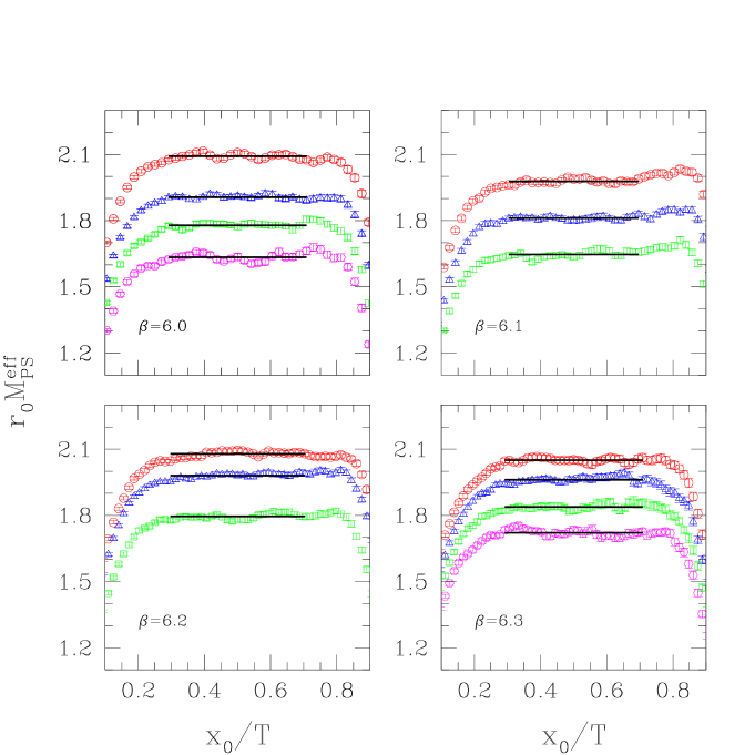
Figure 2: Plateaux for the extraction of $M_{\rm PS}^{\rm eff}$ at $\alpha=\pi/2$. The time-range and value of each plateau is indicated by a straight line segment.

In order to determine the plateaux of the effective masses we have followed the procedure of ref. [31]. We have allowed for a relative excited state contribution to the effective mass of at most $0.2\%$ within the plateaux. The plateaux of the effective masses $[x_{0}^{\rm min}/r_{0},x_{0}^{\rm max}/r_{0}]$, which satisfy this criterion, are listed in Table 2 and illustrated in Fig. 2. The values for $x_{0}^{\rm min}/r_{0}$ indicate that the K-meson decay channel dominates the excited states after roughly $1.25-1.35~{}{\rm fm}$ from the $x_{0}=0$ wall source. The pseudoscalar meson mass $aM_{\rm PS}$ is obtained by averaging the $aM^{\rm eff}_{\rm PS}(x_{0})$ values in the plateaux; errors are estimated by the jackknife procedure, omitting one measurement from each bin. We present this result in the form $r_{0}M_{\rm PS}$ in Table 2.

Given these considerations, we determine $B_{K}$ by averaging in the symmetric interval $[x_{0}^{\rm min}/r_{0},(T-x_{0}^{\rm min})/r_{0}]$. What we compute is the quantity $R_{B}\equiv\hat{R}_{B}/Z_{\rm VA+AV}$ (cf. Eqs. (3.60,3.61, 3.62)), corresponding to the bare $B_{K}$. We distinguish three sources of uncertainty in our $R_{B}$ results:

1. The results depend on the prescription used for the determination of the normalisation constants $Z_{\rm A}$ and $Z_{\rm V}$, as well as the improvement coefficient $c_{\rm\scriptscriptstyle A}$. As discussed in Appendix A, two such independent determinations have been provided by the ALPHA  [38, 39] and LANL [40, 41] collaborations. We compute the ratio $R_{B}$ for both sets of values. The discrepancy between the two determinations is a measure of $O(a^{2})$ systematic effects. We also compute $R_{B}$ with the ALPHA collaboration estimates for $Z_{\rm A}$ and $Z_{\rm V}$, but without the improving $c_{\rm\scriptscriptstyle A}$ counterterm in the axial current. Any discrepancy between this and the previous determinations of $R_{B}$ signals the presence of strong ${\rm O}(a)$ effects.

2. The statistical errors of the correlation functions are computed by a standard jackknife error analysis (omitting one measurement from each bin), without taking into account the errors of $Z_{\rm A}$, $c_{\rm\scriptscriptstyle A}$ and $Z_{\rm V}$.

3. The total statistical error is computed by combining the statistical errors of $Z_{\rm A}$, $Z_{\rm V}$ (for a given ALPHA or LANL determination) with those of the correlation functions, through the standard error propagation procedure. The statistical error of $c_{\rm\scriptscriptstyle A}$ is not taken into account, as it is related to an ${\rm O}(a)$ correction (recall that for the same reason, $c_{\rm sw}$ is also used without an error).

$\beta$	$\big{[}\dfrac{x_{0}^{\rm min}}{2r_{0}},\dfrac{x_{0}^{\rm max}}{2r_{0}}\big{]}$	$r_{0}M_{\rm PS}$	$R_{B}^{\rm ALPHA}$	$R_{B}^{\rm LANL}$	$R_{B}^{{\rm ALPHA;~{}w/o}~{}c_{\rm\scriptscriptstyle A}}$
6.0	$[1.30,3.17]$	2.092(6)	1.177(9)(8)(12)	1.089(8)(11)(14)	1.025(8)(6)(10)
		1.907(7)	1.139(13)(8)(15)	1.054(12)(11)(16)	0.993(12)(6)(13)
		1.780(6)	1.123(14)(8)(16)	1.038(12)(11)(16)	0.977(12)(6)(13)
		1.635(6)	1.084(13)(8)(15)	1.001(12)(10)(16)	0.943(11)(5)(12)
		1.2544	1.031(19)(23)	0.952(17)(24)	0.896(16)(18)
6.1	$[1.34,3.08]$	1.978(6)	1.066(9)(8)(12)	1.041(8)(7)(11)	0.992(8)(6)(10)
		1.812(7)	1.023(10)(7)(12)	0.998(10)(6)(12)	0.951(9)(6)(11)
		1.647(6)	0.981(10)(7)(12)	0.955(10)(6)(12)	0.911(9)(5)(10)
		1.2544	0.901(21)(25)	0.874(20)(25)	0.835(18)(21)
6.2	$[1.29,3.05]$	2.079(6)	1.023(7)(7)(10)	1.017(7)(8)(11)	0.980(7)(6)(9)
		1.980(7)	0.993(9)(7)(11)	0.987(9)(7)(11)	0.951(8)(5)(9)
		1.795(7)	0.975(8)(7)(11)	0.970(8)(7)(11)	0.935(8)(5)(9)
		1.2544	0.902(23)(31)	0.900(23)(32)	0.868(23)(26)
6.3	$[1.23,3.00]$	2.050(6)	0.990(12)(7)(14)	0.996(12)(5)(13)	0.962(12)(5)(13)
		1.962(8)	0.996(15)(7)(17)	1.003(15)(5)(16)	0.967(14)(5)(15)
		1.839(10)	0.959(17)(7)(18)	0.964(17)(5)(18)	0.932(16)(5)(17)
		1.722(9)	0.918(15)(6)(16)	0.924(15)(5)(16)	0.892(14)(5)(15)
		1.2544	0.844(32)(35)	0.851(32)(34)	0.820(30)(33)

Table 2: Results for the pseudoscalar mass and the various ratios from which $B_{K}$ is extracted (twist angle $\alpha=\pi/2$). The error in $r_{0}M_{\rm PS}$ is statistical. The three errors of the $R_{B}$ ratio are, in order of appearance: (i) due to the statistical fluctuations of the correlations; (ii) due to the errors of $Z_{\rm A,V}$; (iii) the total error from the two previous ones. The results of the extrapolations to the physical Kaon mass values are shown at the bottom of each $\beta$-dataset: the first error of $R_{B}$ is that arising from type-(i) errors of the fitted values, while the second is from type-(iii) errors.

The results for $R_{B}$ (and pseudoscalar masses) are collected in Table 2. They have all been computed at the time-plateaux shown in the second column, determined from the effective mass of Eq. (4.66) with ALPHA collaboration values for $Z_{\rm A}$, $Z_{\rm V}$ and $c_{\rm\scriptscriptstyle A}$. The quality of the data is also illustrated in Fig. 2. It is clear that as the continuum limit is approached, the $O(a^{2})$ discrepancies between $R_{B}^{\rm ALPHA}$ and $R_{B}^{\rm LANL}$ tend to decrease. This tendency is less marked for $R_{B}^{{\rm ALPHA~{}w/o}~{}c_{\rm\scriptscriptstyle A}}$, which differs from the other two by ${\rm O}(a)$ effects.

The $R_{B}$ values are extrapolated linearly in $(r_{0}M_{\rm PS})^{2}$, to the physical point $(r_{0}M_{K})^{2}=1.5736$ (corresponding to $M_{K}^{2}={\scriptstyle{{1\over 2}}}[M_{K^{0}}^{2}+M_{K^{\pm}}^{2}]$), see Fig. 6. An interesting issue concerns the magnitude of the error of these extrapolated values. Usually, in quenched simulations performed at a given $\beta$, observables such as the ratio $R_{B}$ are computed on the same configuration ensemble for all values of the bare quark masses (hopping parameters). This means that the extrapolation to the strange quark mass is performed on data points which are strongly correlated, thus reducing the error of the extrapolation. We have instead opted for independent Monte Carlo simulations for each set of bare quark masses, which in this respect mimic unquenched simulations, at the price of having uncorrelated $R_{B}$ results with larger errors on the extrapolations.

The justification of the linear fit of $R_{B}$, as a function of the squared pseudoscalar mass is provided in Appendix C.

4.1 Finite volume effects

In order to investigate finite volume effects, we have performed a simulation at $\beta=6.0$ for a larger spatial volume, with extension $L/a=24$, at the lightest mass $r_{0}M_{\rm PS}=1.635$. The results are gathered in Table 3.

$L^{3}\times T/a^{4}$	$r_{0}M_{\rm PS}$	$R_{B}^{\rm ALPHA}$	$N_{\rm conf}$
$16^{3}\times 48$	1.635(6)	1.084(13)(8)(15)	400
$24^{3}\times 48$	1.624(5)	1.079(7)(8)(11)	167

Table 3: $B_{K}$-parameter at fixed effective pseudoscalar mass $M_{\rm PS}^{\rm eff}$ for two different spatial lattice volumes (twist angle $\alpha=\pi/2$). The various errors on $R_{B}$ are explained in the caption of Table 2.

Finite volume effects are estimated in terms of the following ratios:

$$\dfrac{M_{\rm PS}(L/a=16)}{M_{\rm PS}(L/a=24)}-1=0.007(5)\,,\qquad\dfrac{R_{B}^{\rm ALPHA}(L/a=16)}{R_{B}^{\rm ALPHA}(L/a=24)}-1=0.005(17)\,.$$ (4.67)

Note that all errors are of purely statistical nature. We see that the effective mass ratios have a very small statistical deviation from zero, while the $B_{K}$ ratio is essentially insensitive to finite volume effects.

4.2 Non-degenerate masses

Past and current simulations for the determination of $B_{K}$ have mostly been carried out with degenerate down and strange quarks. The rationale behind this (at least as far as quenched simulations are concerned) is to be found in the chiral perturbation theory expression for $B_{K}$. As discussed in ref. [19, 20, 21, 22], the quenched chiral expression for $B_{K}$ is given by

$$B_{K}=B\Big{[}1-(3+\epsilon^{2})y\ln y+by+cy\epsilon^{2}+\delta\Big{\{}\dfrac{2-\epsilon^{2}}{2\epsilon}\ln\left(\dfrac{1-\epsilon}{1+\epsilon}\right)+2\Big{\}}\Big{]}\,,$$ (4.68)

with $y=m_{K}^{2}/(4\pi F)^{2}$ and $F\simeq 102$ MeV (see ref. [43]). The parameter

$$\epsilon\equiv\dfrac{m_{s}-m_{d}}{m_{s}+m_{d}}$$ (4.69)

is a measure of the down-strange degeneracy breaking. The expression (4.68) is identical in form to the one valid for dynamical quarks, save for the $\delta-$term. This quenched artefact vanishes in the degenerate limit $\epsilon\rightarrow 0$, but diverges when the down quark becomes chiral and $\epsilon\rightarrow 1$.

We have measured $R_{B}$ with non-degenerate down and strange quarks. Our aim is to probe its dependence on quark mass differences, while avoiding the potentially dangerous $\epsilon\rightarrow 1$ limit. We have performed runs at $\beta=6.0$, for two values of $\epsilon\neq 0$, tuning the bare mass parameters so that the pseudoscalar mass remains close to the value $r_{0}M_{\rm PS}=1.780$ of the $\epsilon=0$ simulation. Our results are summarised in Table 4.

$\epsilon$	$\kappa_{s}$	($\kappa_{d}$,$a\mu$)	$r_{0}M_{\rm PS}$	$R_{B}^{\rm ALPHA}$	$N_{\rm conf}$
0.00	0.1340	(0.1351830,0.02708)	1.780(6)	1.123(14)(8)(16)	400
0.16	0.1338	(0.1351867,0.02259)	1.775(6)	1.128(17)(8)(19)	400
0.41	0.1335	(0.1351913,0.01598)	1.772(7)	1.129(14)(8)(16)	402

Table 4: $B_{K}$-parameter at fixed effective pseudoscalar mass $M_{\rm PS}^{\rm eff}$ for three values of the degeneracy-breaking parameter $\epsilon$ (twist angle $\alpha=\pi/2$). The various errors on $R_{B}$ are explained in the caption of Table 2.

The effect of breaking the mass degeneracy of the valence quarks is estimated in terms of the following ratios:

$$\dfrac{M_{\rm PS}(\epsilon=0)}{M_{\rm PS}(\epsilon=0.16)}-1 =0.003(5), \dfrac{M_{\rm PS}(\epsilon=0)}{M_{\rm PS}(\epsilon=0.41)}-1 =0.005(5),$$ (4.70)

$$\dfrac{\ \ R_{B}^{\rm ALPHA}(\epsilon=0)\ \ }{R_{B}^{\rm ALPHA}(\epsilon=0.16)}-1 =-0.004(19), \dfrac{\ \ R_{B}^{\rm ALPHA}(\epsilon=0)\ \ }{R_{B}^{\rm ALPHA}(\epsilon=0.41)}-1 =-0.005(17).$$ (4.71)

All errors are statistical. We see that there is no appreciable deviation between $\epsilon=0$ and $\epsilon\neq 0$ values. It seems that, at least in the region of mass differences explored, $B_{K}$ is not sensitive to the breaking of mass degeneracy.

Finally, we find it worth to mention in this context a curious by-product of our computations that concerns the somewhat surprising appearance of an exceptional configuration in the $\pi/2$ simulation with non-twisted strange valence quarks, corresponding to a rather heavy $K$-meson of $m_{K}\simeq 650$ MeV. This happened at $\beta=6.0$ and for a “standard” value of the Wilson hopping parameter which, being generally considered “safe” from exceptional configurations, has also been used in the simulations of other collaborations. More details are provided in Appendix D.

5 Lattice $B_{K}$ results from tmQCD at $\alpha=\pi/4$

$\beta$	$(L/a)^{3}\times T/a$	$a\over 2r_{0}$	$L\over 2r_{0}$	$(\kappa,a\mu)$	$N_{\rm conf}$
6.00	$24^{3}\times 48$	0.0931	2.24	(0.134739,0.010412)	200
				(0.134795,0.009142)
				(0.134828,0.008397)
6.10	$24^{3}\times 60$	0.0789	1.89	(0.135152,0.00810)	200
				(0.135190,0.00720)
				(0.135235,0.00615)
6.20	$32^{3}\times 72$	0.0677	2.17	(0.135477,0.007595)	73
				(0.135539,0.006125)
6.30	$32^{3}\times 72$	0.0587	1.88	(0.135509,0.0076)	76
				(0.135546,0.0067)
				(0.135584,0.0058)
6.45	$32^{3}\times 86$	0.0481	1.54	(0.135105,0.01459)	105
				(0.135218,0.01185)
				(0.135293,0.01002)

Table 5: The parameters of the runs at twist angle $\alpha=\pi/4$.

$\beta$	$\big{[}\dfrac{x_{0}^{\rm min}}{2r_{0}},\dfrac{x_{0}^{\rm max}}{2r_{0}}\big{]}$	$r_{0}M_{\rm PS}$	$R_{B}^{\rm ALPHA}$	$R_{B}^{\rm LANL}$	$R_{B}^{{\rm ALPHA;~{}w/o}~{}c_{\rm\scriptscriptstyle A}}$
6.0	$[1.30,3.17]$	1.326(4)	1.067(8)(8)(11)	0.960(7)(10)(12)	0.885(6) (5)(8)
	$[1.30,3.17]$	1.253(4)	1.048(8)(7)(11)	0.941(7)(9)(11)	0.868(7) (5)(9)
	$[1.30,3.17]$	1.207(4)	1.036(9)(7)(11)	0.930(8)(9)(12)	0.857(7) (5)(9)
		1.2544	1.048(8)(11)	0.943(7)(12)	0.869(7)(9)
6.1	$[1.18,3.55]$	1.381(5)	0.912(8)(7)(11)	0.883(8)(6)(10)	0.829 (8)(5)(9)
	$[1.18,3.55]$	1.325(5)	0.892(9)(6)(11)	0.863(9)(6)(11)	0.810 (8)(5)(9)
	$[1.26,3.47]$	1.257(5)	0.865(10)(6)(12)	0.836(9)(6)(11)	0.785 (9)(5)(10)
		1.2544	0.865(10)(11)	0.836(9)(11)	0.784(9)(10)
6.2	$[1.35,3.52]$	1.299(6)	0.882(11)(6)(13)	0.875(11)(6)(13)	0.831 (10)(5)(11)
	$[1.35,3.52]$	1.182(6)	0.852(12)(6)(13)	0.845(12)(6)(13)	0.803 (11)(5)(12)
		1.2544	0.869(11)(13)	0.863(10)(12)	0.818(10)(11)
6.3	$[1.29,2.94]$	1.338(9)	0.848(13)(6)(14)	0.854(13)(5)(14)	0.815 (12)(5)(13)
	$[1.35,2.88]$	1.259(9)	0.831(14)(6)(15)	0.835(14)(5)(15)	0.798 (13)(5)(14)
	$[1.47,2.76]$	1.175(10)	0.811(15)(6)(16)	0.814(14)(5)(15)	0.779 (14)(4)(15)
		1.2544	0.829(13)(14)	0.834(13)(14)	0.797(12)(13)
6.45	$[1.30,2.84]$	2.054(10)	0.937(11)(7)(13)	0.949(10)(6)(13)	0.913 (10)(5)(11)
	$[1.25,2.88]$	1.848(11)	0.904(12)(6)(13)	0.915(12)(6)(13)	0.881 (11)(5)(12)
	$[1.30,2.84]$	1.702(11)	0.879(13)(6)(14)	0.889(13)(6)(14)	0.856 (13)(5)(14)
		1.2544	0.821(16)(18)	0.831(16)(17)	0.800(16)(17)

Table 6: Results for the pseudoscalar mass and the various ratios from which $B_{K}$ is extracted (twist angle $\alpha=\pi/4$). The error in $r_{0}M_{\rm PS}$ is statistical. The three errors of the $R_{B}$ ratio are, in order of appearance: (i) due to the statistical fluctuations of the correlations; (ii) due to the errors of $Z_{\rm A,V}$; (iii) the total error from the two previous ones. The results of the extrapolations to the physical Kaon mass values are shown at the bottom of each $\beta$-dataset: the first error of $R_{B}$ is that arising from type-(i) errors of the fitted values, while the second is from type-(iii) errors.

The quenched $B_{K}$ parameter has also been computed in tmQCD with a twist angle $\alpha=\pi/4$. This formalism, with twisted down and strange quarks in the same flavour doublet, is a way to avoid the problem of exceptional configurations, while maintaining the property of multiplicative renormalisation of the four-fermion operator. Therefore, contrary to the $\alpha=\pi/2$ simulation, in the present one it is possible to simulate at half the value of the physical strange quark mass directly, thus avoiding the uncertainties introduced by extrapolations from higher masses. The price to pay is that larger physical volumes are required at these smaller masses. Our simulations have been performed at four values of the lattice spacing in the range $a\approx 0.05-0.09~{}{\rm fm}$, while lattice spatial extensions are $L\approx 1.9-2.2~{}{\rm fm}$. Time ranges from $x_{0}=0$ to $x_{0}=T$, with $T/L\geq 2$. The two mass parameters (hopping parameter $\kappa$ and twisted mass $\mu$ for the two degenerate valence flavours) are tuned as discussed in sect. 2. Contrary to the $\pi/2$ case, here we have generated a single configuration ensemble per $\beta$, on which measurements at a few $(\kappa,a\mu)$ values, tuned to be close to half the strange quark mass, are performed. The parameters of our runs are displayed in Table 5. We point out that at the smallest lattice spacing, corresponding to $\beta=6.45$, APEmille memory limitations made it impossible to maintain the physical volume used at the lower $\beta$ values. Consequently, in this case we were forced to run at a length of $L\approx 1.5~{}{\rm fm}$, with larger masses, and extrapolate to the pseudoscalar mass at the physical kaon mass.

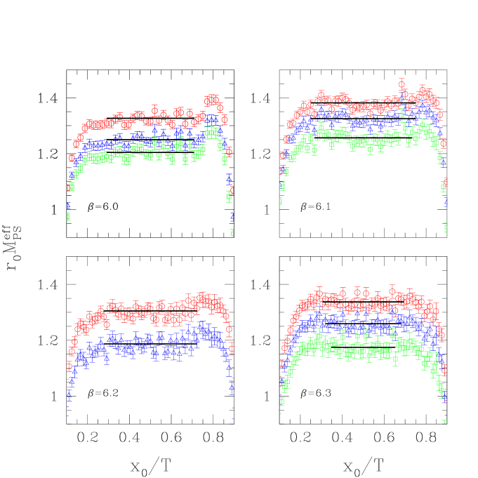
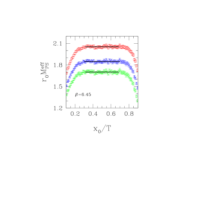
Figure 3: Plateaux for the extraction of $M_{\rm PS}^{\rm eff}$ at $\alpha=\pi/4$. The time-range and value of each plateau is indicated by a straight line segment.

The effective pseudoscalar meson mass is computed from the ratio of Eq. (4.66); again correlation functions are antisymmetrised in time. The excited states analysis, carried out as in ref. [44], determines the effective mass plateaux for which the relative contribution from the excited states is at most $0.5\%$. The plateaux of the effective masses $[x_{0}^{\rm min}/r_{0},x_{0}^{\rm max}/r_{0}]$ are listed in Table 6 and illustrated in Fig. 3. Once more, they have been obtained with the ALPHA collaboration values for $Z_{\rm A}$, $Z_{\rm V}$ and $c_{\rm\scriptscriptstyle A}$. The quoted values for $x_{0}^{\rm min}/r_{0}$ indicate that the K-meson channel dominates the excited states after roughly $1.2$ to $1.4~{}{\rm fm}$ from the $x_{0}=0$ wall source. The pseudoscalar meson mass $aM_{\rm PS}$ is obtained by averaging the $aM^{\rm eff}_{\rm PS}(x_{0})$ values in the plateaux; errors are estimated by the jackknife procedure, omitting one measurement from each bin. This result is presented in the form $r_{0}M_{\rm PS}$ in Table 6.

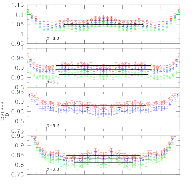
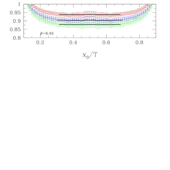
Figure 5: Plateaux for the extraction of $R_{\rm B}^{\rm ALPHA}$ at $\alpha=\pi/4$. The time-range and value of each plateau is indicated by a straight line segment.

The ratio $R_{B}$ is computed in the symmetric interval $[x_{0}^{\rm min}/r_{0},(T-x_{0}^{\rm min})/r_{0}]$. The results for $R_{B}$ are collected in Table 6. We see once more that as the continuum limit is approached, the $O(a^{2})$ discrepancies between $R_{B}^{\rm ALPHA}$ and $R_{B}^{\rm LANL}$ tend to decrease. This tendency is less marked for $R_{B}^{{\rm ALPHA~{}w/o}~{}c_{\rm\scriptscriptstyle A}}$, which differs from the other two by ${\rm O}(a)$ effects. The plateaux from which $B_{K}$ is extracted are illustrated in Fig. 5.

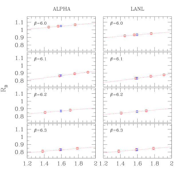
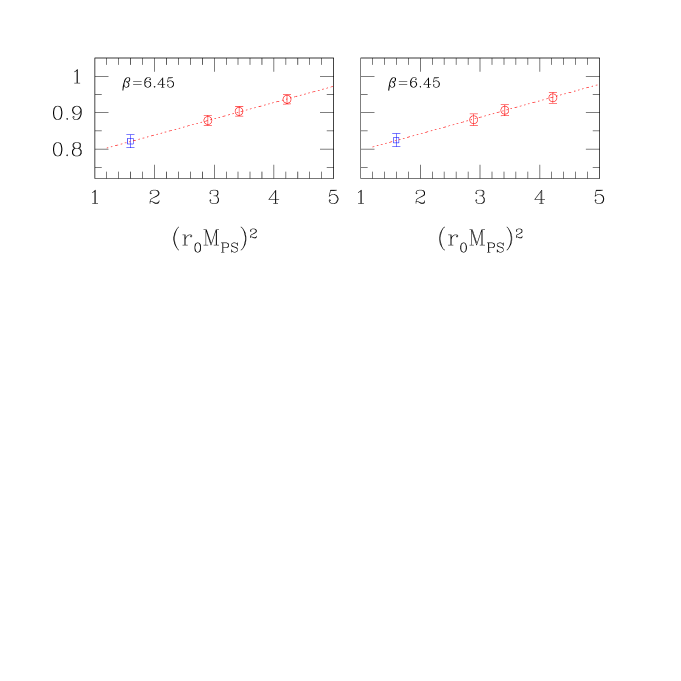
Figure 7: Linear inter/extrapolation of $R_{\rm B}$ to the physical kaon mass at $\alpha=\pi/4$.

The $R_{B}$ values are interpolated linearly in $(r_{0}M_{\rm PS})^{2}$, to the physical point $(r_{0}M_{K})^{2}=1.5736$, see Fig. 7. These interpolations are very short and involve data which, having been obtained at the same configuration ensemble, are correlated. Thus, the error on the interpolated value, compared to the one obtained in the $\alpha=\pi/2$ case by extrapolation from higher pseudoscalar masses, is smaller. For the $\beta=6.45$ case, we still have correlated data, but as the physical value is reached by an extrapolation, the error is relatively large.

5.1 Finite volume effects

In order to test finite volume effects, we have performed simulations at $\beta=6.0,6.1,6.2$ for various spatial volumes and light quark masses. The simulation points, as well as the results for the pseudoscalar meson mass and for $R_{B}$, are gathered in Table 7. The spatial extent of the lattices considered roughly ranges from $1.5$ to $3.0$ fm.

$\beta$	$L^{3}\times T/a^{4}$	$\dfrac{L}{2r_{0}}$	$\dfrac{T}{2r_{0}}$	$(\kappa,a\mu)$	$r_{0}M_{\rm PS}$	$R_{B}^{\rm ALPHA}$	$N_{\rm conf}$
6.0	$16^{3}\times 48$	1.488	4.464	$(0.134739,0.010412)$	1.316(5)	1.040(11)(7)(13)	667
	$16^{3}\times 48$	1.488	4.464	$(0.134828,0.008397)$	1.196(6)	0.999(13)(7)(15)	667
	$24^{3}\times 48$	2.232	4.464	$(0.134739,0.010412)$	1.326(4)	1.067(8)(8)(11)	200
	$24^{3}\times 48$	2.232	4.464	$(0.134828,0.008397)$	1.207(4)	1.036(9)(7)(11)	200
	$32^{3}\times 60$	2.976	5.580	$(0.134828,0.008397)$	1.201(3)	1.035(6)(7)(9)	76
6.1	$24^{3}\times 60$	1.896	4.740	$(0.135152,0.008100)$	1.381(5)	0.912(8)(7)(11)	200
	$24^{3}\times 60$	1.896	4.740	$(0.135235,0.006150)$	1.257(5)	0.865(9)(6)(11)	200
	$32^{3}\times 64$	2.528	5.056	$(0.135152,0.008100)$	1.370(5)	0.925(7)(7)(10)	77
	$32^{3}\times 64$	2.528	5.056	$(0.135235,0.006150)$	1.245(5)	0.876(8)(6)(10)	77
6.2	$24^{3}\times 72$	1.620	4.860	$(0.135477,0.007595)$	1.298(8)	0.853(16)(6)(17)	191
	$24^{3}\times 72$	1.620	4.860	$(0.135539,0.006125)$	1.182(9)	0.813(18)(6)(19)	191
	$32^{3}\times 72$	2.160	4.860	$(0.135477,0.007595)$	1.299(6)	0.882(11)(6)(13)	73
	$32^{3}\times 72$	2.160	4.860	$(0.135539,0.006125)$	1.182(6)	0.852(12)(6)(13)	73

Table 7: $B_{K}$ parameter (at two values of the effective pseudoscalar mass $M_{\rm PS}$ per $\beta$) for different spatial lattice volumes (twist angle $\alpha=\pi/4$). The various errors on $R_{B}$ are explained in the caption of Table 6.

The usual $M_{\rm PS}$ and $R_{B}^{\rm ALPHA}$ ratios at two different spatial volumes are computed at fixed $\beta$ and their deviation from unity is presented in Table 8.

For $\beta=6.0,6.1$ the effective mass ratios display some small finite volume effects, at $L\sim 1.5$ fm to $2$ fm, which appear to vanish at $L\sim 2.5$ fm. For $\beta=6.2$ however, such effects are also absent already at $L\sim 1.5$ fm. It has to be noted, however, that at this level of precision it is difficult to disentangle finite volume effects from e.g. the difference in cutoff effects, or the systematic uncertainties related to excited states.

For $B_{K}$ we see finite volume effects at $L\sim 1.5$ fm, which disappear at $L\sim 2$ fm. This situation is $\beta$-independent.

$\beta$	$\dfrac{L_{1}}{a}$	$\dfrac{L_{2}}{a}$	$\dfrac{L_{1}}{2r_{0}}$	$\dfrac{L_{2}}{2r_{0}}$	$(\kappa,a\mu)$	$\left[\dfrac{M_{\rm PS}(L_{1})}{M_{\rm PS}(L_{2})}-1\right]$	$\left[\dfrac{R_{B}^{\rm ALPHA}(L_{1})}{R_{B}^{\rm ALPHA}(L_{2})}-1\right]$
6.0	16	24	1.488	2.232	$(0.134739,0.010412)$	-0.008(5)	-0.023(16)
					$(0.134828,0.008397)$	-0.009(6)	-0.033(18)
	24	32	2.232	2.976	$(0.134828,0.008397)$	0.005(4)	-0.002(14)
6.1	24	32	1.896	2.528	$(0.135152,0.008100)$	0.008(5)	-0.014(16)
					$(0.135235,0.006150)$	0.010(6)	0.014(17)
6.2	24	32	1.620	2.160	$(0.135477,0.007595)$	-0.001(8)	-0.032(23)
					$(0.135539,0.006125)$	0.000(10)	-0.046(26)

Table 8: Finite volume effects for pseudoscalar masses $M_{\rm PS}$ and $B_{K}$ parameters (twist angle $\alpha=\pi/4$). The errors are statistical.

6 $B_{K}$ in the continuum limit

Having obtained the value of the bare $B_{K}$ parameter at several lattice spacings, we now proceed to the computation of its renormalised counterpart in the continuum limit. In ref. [13], the necessary renormalisation constants have been calculated non-perturbatively in various Schrödinger functional schemes, as well as the operator step scaling functions, which determine its renormalisation group running. What we need from ref. [13] is the total renormalisation factor $\mathcal{Z}_{\rm VA+AV;}^{+}(g_{0})$, which connects the bare $B_{K}$ to its RGI value as follows:

$$\hat{B}_{K}=\lim_{g_{0}\rightarrow 0}\,\,\,\mathcal{Z}_{\rm VA+AV;s}^{+}(g_{0})\,\,\,B_{K}(g_{0})\,.$$ (6.72)

The bare $B_{K}(g_{0})$ is given by $R_{B}$ at the physical point $r_{0}M_{K}$ (see Tables 2 and 6). Which of the three candidates $R_{B}^{\rm ALPHA}$, $R_{B}^{\rm LANL}$ or $R_{B}^{{\rm ALPHA;~{}w/o}~{}c_{\rm\scriptscriptstyle A}}$ is most suitable will be discussed below. The quantity $\mathcal{Z}_{\rm VA+AV;s}^{+}$ is the product of three factors: (i) the operator renormalisation constant $Z_{\rm VA+AV;s}^{+}(g_{0},a\mu_{\rm min})$ at a hadronic scale $\mu_{\rm min}$; (ii) the RG-running evolution function from the scale $\mu_{\rm min}$ to a (hopefully) perturbative scale $\mu_{\rm max}=2^{7}\mu_{\rm min}$; (iii) the RG evolution function from the scale $\mu_{\rm max}$ to infinity. For several SF renormalisation schemes, the first two factors are known non-perturbatively (see ref. [13]), while the third is known in NLO perturbation theory (see ref. [45]). Following ref. [13] we write

$$\mathcal{Z}_{\rm VA+AV;s}^{+}(g_{0})=\hat{Z}_{\rm VA+AV;s}^{+}(\mu_{\rm min})\,Z_{\rm VA+AV;s}^{+}(g_{0},a\mu_{\rm min})\,,$$ (6.73)

where $\hat{Z}_{\rm VA+AV;s}^{\pm}(\mu_{\rm min})$ is the product of the two evolution functions.

Note that $\mathcal{Z}_{\rm VA+AV;s}^{+}(g_{0})$ depends on the renormalisation scheme $s$ only via cutoff effects. In refs. [13] and [45], nine variants of Schrödinger functional frameworks have been explored, each giving rise to a distinct renormalisation scheme $s$. Three of these schemes have been deemed “reliable”, essentially because they display the best control of the systematic uncertainty due to the use of NLO perturbation theory in the calculation of $\mathcal{Z}_{\rm VA+AV;s}^{+}$. We refer the reader to ref. [13] for details; here we just state that, following this work we label these schemes as $s=1,3,7$.

Given the different origin of the factors contriving to give $\hat{B}_{K}$, the extraction of its error is somewhat intricate. The values of $\mathcal{Z}_{\rm VA+AV;s}^{+}(g_{0})$ for the couplings of interest are collected in Table 12 of Appendix A, where a $1\%$ error is quoted. This error is only due to the uncertainties in the determination of the lattice renormalisation constant $Z_{\rm VA+AV;s}^{+}(g_{0},a\mu_{\rm min})$. It is combined in quadrature with the error for the bare $B_{K}(g_{0})$ (given in Tables 2 and 6) in order to give the uncertainty for $\hat{B}_{K}$, at each $\beta$ value. Our results for $\hat{B}_{K}$ (from $R_{B}^{\rm ALPHA}$), with the error obtained as described, are gathered in Table 9. Once these results are extrapolated to the continuum limit, a further error has to be added in quadrature, due to the evolution function $\hat{Z}_{\rm VA+AV;s}^{\pm}(\mu_{\rm min})$; the reason this is only done at the very end is that the evolution function is a continuum quantity. As reported in ref. [13], the relative error of $\hat{Z}_{\rm VA+AV;s}^{\pm}(\mu_{\rm min})$ is $2\%$.

From the results of Table 9 we see that $\hat{B}_{K}$ is essentially independent of the scheme $s$. In the remaining analysis, we will only consider the $s=1$ results. This arbitrary choice does not introduce any loss of generality.

$\beta$	6.0	6.1	6.2	6.3	6.45
$s=1$	0.911(22)	0.812(24)	0.828(30)	0.789(34)	—
$s=3$	0.918(22)	0.816(24)	0.831(30)	0.791(34)	—
$s=7$	0.913(22)	0.814(24)	0.830(30)	0.791(34)	—
$\beta$	6.0	6.1	6.2	6.3	6.45
$s=1$	0.926(13)	0.779(13)	0.798(14)	0.775(15)	0.789(19)
$s=3$	0.933(14)	0.783(13)	0.800(14)	0.777(15)	0.789(19)
$s=7$	0.929(13)	0.781(13)	0.799(14)	0.777(15)	0.790(19)

Table 9: The value of $\hat{B}_{K}$ at fixed $\beta$-coupling, obtained from three distinct Schrödinger functional renormalisation schemes $s$. The quoted error combines in quadrature the uncertainty in the computation of the bare $B_{K}$-parameter and that of the total renormalisation factor $\mathcal{Z}_{\rm VA+AV;s}^{+}(g_{0})$. The upper part of the table refers to $\alpha=\pi/2$ results, while the lower part to $\alpha=\pi/4$.

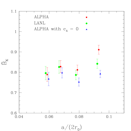
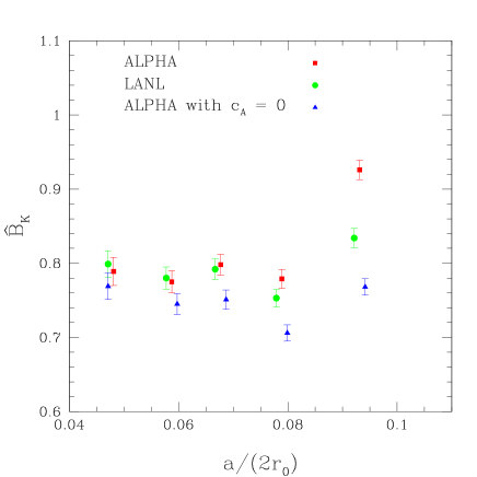
Figure 8: Comparison of $\hat{B}_{K}$, extracted from three different definitions of $R_{\rm B}$, differing by the axial currents’ ${\rm O}(a)$ counterterms. Top: results for $\alpha=\pi/2$. Bottom: results for $\alpha=\pi/4$.

Next we explore the influence of the different choices of axial currents in the determination of $\hat{B}_{K}$. This entails comparing results extracted from $R_{B}^{\rm ALPHA}$, $R_{B}^{\rm LANL}$ and $R_{B}^{{\rm ALPHA;~{}w/o}~{}c_{\rm\scriptscriptstyle A}}$; see Fig. 8. Not surprisingly, the $\pi/2$ data is noisier than that of $\pi/4$. This is due to the fact that the latter dataset has been produced without extrapolations in the K-meson mass. The comparison between $R_{B}^{\rm ALPHA}$ and $R_{B}^{{\rm ALPHA;~{}w/o}~{}c_{\rm\scriptscriptstyle A}}$ (which have the same $Z_{\rm A}$) shows that there are large $c_{\rm\scriptscriptstyle A}$-related cutoff effects at $\beta=6.0$, which diminish as $\beta$ increases. The $R_{B}^{\rm LANL}$ points fall in-between these two cases. Once the $\beta=6.0$ data, afflicted by large discretisation effects, are conservatively discarded, we are faced with three $B_{K}$ estimates which display reasonable scaling behaviour. At the largest $\beta$ values, the three $B_{K}$ results are perfectly compatible. In trying to decide which is the most reliable, we recall that the ALPHA and LANL $Z_{\rm A}$ values have been obtained for an axial current which contains the $c_{\rm\scriptscriptstyle A}$ counterterm. Thus, the fact that $R_{B}^{{\rm ALPHA;~{}w/o}~{}c_{\rm\scriptscriptstyle A}}$ contains the ALPHA $Z_{\rm A}$ without the $c_{\rm\scriptscriptstyle A}$ counterterm is somewhat un-natural but not illicit, as it only re-introduces ${\rm O}(a)$ effects in the axial current. It could even be the source of beneficial correlators in the $B_{K}$ ratio, as the corresponding $O_{\rm VA+AV}$ counterterms are also missing in the numerator. Nevertheless, the $R_{B}^{{\rm ALPHA;~{}w/o}~{}c_{\rm\scriptscriptstyle A}}$ results would have been on a firmer ground, had they been obtained with an independent $Z_{\rm A}$ determination from Ward identities, with the Clover action and without the $c_{\rm\scriptscriptstyle A}$ term. Also the $R_{B}^{\rm LANL}$ dataset is clearly of somewhat inferior quality, as the $Z_{\rm A}$ and $c_{\rm\scriptscriptstyle A}$ are only given at a few $\beta$ values in ref. [41], while for the other $\beta$’s we had to use simple extrapolations (cf. Table 11). These general considerations place the $R_{B}^{\rm ALPHA}$ result on firmer ground and justify taking the $R_{B}^{\rm ALPHA}$ dataset (without the $\beta=6.0$ point) as our best candidate for a precision measurement of $B_{K}$ in the continuum limit.

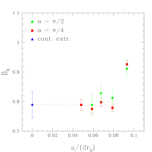
Figure 9: Continuum limit extrapolation of $\hat{B}_{K}$, obtained from a combined linear fit of the $\alpha=\pi/2$ and $\alpha=\pi/4$ data. The coarsest lattice data, corresponding to $\beta=6.0$, is not included in the fit.

A further important element is the choice of extrapolating function. On one hand we know that ${\rm O}(a)$ effects are present and a linear extrapolation would be theoretically justified, which however would amplify the final error. This is especially true for our results obtained with $\alpha=\pi/2$, which have rather large errors. On the other hand, we see that our data points show an essentially constant behaviour in $\beta$, supporting a constant fit on empirical grounds, which would give smaller errors. The procedure which is theoretically sound, while keeping errors under control, is a combined linear fit of the $\alpha=\pi/2$ and $\alpha=\pi/4$ results, constraining $\hat{B}_{K}$ to a unique value in the continuum limit. Following this procedure (see Fig. 9) we arrive at our final result:

$$\hat{B}_{K}=0.789\pm 0.046\,.$$ (6.74)

It is nevertheless customary to quote $B_{K}$ also in the ${\rm\overline{MS\kern-0.50003pt}\kern 0.50003pt}$ scheme at a scale $\mu=2~{}{\rm GeV}$. The relation between $\hat{B}_{K}$ and $B_{K}^{{\rm\overline{MS\kern-0.35002pt}\kern 0.35002pt}}(\mu)$ is known at NLO (we follow the notation of [45, 13]):

$$\hat{B}_{K} = \Big{[}\dfrac{{\bar{g}}^{2}(\mu)}{4\pi}\Big{]}^{-\dfrac{\gamma^{+}_{0}}{2b_{0}}}\,\,\exp\Big{[}-\int_{0}^{{\bar{g}}(\mu)}dg\,\Big{(}\dfrac{\gamma^{+}(g)}{\beta(g)}-\dfrac{\gamma^{+}_{0}}{b_{0}g}\Big{)}\Big{]}B_{K}^{{\rm\overline{MS\kern-0.35002pt}\kern 0.35002pt}}(\mu)$$ (6.75)

$$\approx \Big{[}\dfrac{{\bar{g}}^{2}(\mu)}{4\pi}\Big{]}^{-\dfrac{\gamma^{+}_{0}}{2b_{0}}}\,\,\Big{[}1-{\bar{g}}^{2}(\mu)\Big{(}\dfrac{\gamma^{+}_{1}b_{0}-\gamma^{+}_{0}b_{1}}{2b_{0}^{2}}\Big{)}\Big{]}B_{K}^{{\rm\overline{MS\kern-0.35002pt}\kern 0.35002pt}}(\mu)\,.$$

The gauge coupling anomalous dimension coefficients $b_{0}$ and $b_{1}$ are universal. The LO operator anomalous dimension coefficient $\gamma^{+}_{0}$ is also universal, while the NLO one $\gamma^{+}_{1}$ depends on the choice of scheme. For ${\rm\overline{MS\kern-0.50003pt}\kern 0.50003pt}$ one also needs to specify the details of the $\gamma_{5}$ matrix regularisation (i.e. DRED, NDR, HV). The values of these coefficients are collected in ref. [45]. Note that in the DRED scheme the renormalised coupling we use is the one defined in the ${\rm\overline{MS\kern-0.50003pt}\kern 0.50003pt}$ scheme (rather than the one used in the original DRED paper of ref. [46]). Our ${\rm\overline{MS\kern-0.50003pt}\kern 0.50003pt}$ results are

$$B_{K}^{{\rm\overline{MS\kern-0.35002pt}\kern 0.35002pt},{\rm DRED}}(2~{}{\rm GeV}) = 0.599(36)\,.$$ (6.76)

$$B_{K}^{{\rm\overline{MS\kern-0.35002pt}\kern 0.35002pt},{\rm NDR}}(2~{}{\rm GeV}) = 0.573(34)\,,$$ (6.77)

$$B_{K}^{{\rm\overline{MS\kern-0.35002pt}\kern 0.35002pt},{\rm HV}}(2~{}{\rm GeV}) = 0.633(38)\,.$$ (6.78)

The errors cited above arise from three uncertainties added in quadrature:

• The $\hat{B}_{K}$ error of Eq. (6.74).

• The uncertainty of $\Lambda_{{\rm\overline{MS\kern-0.35002pt}\kern 0.35002pt}}$, related to the renormalisation group running of $\bar{g}^{2}_{{\rm\overline{MS\kern-0.35002pt}\kern 0.35002pt}}$. We have used $r_{0}\Lambda_{{\rm\overline{MS\kern-0.35002pt}\kern 0.35002pt}}=0.602(48)$ from [47] to find $\bar{g}^{2}_{{\rm\overline{MS\kern-0.35002pt}\kern 0.35002pt}}(2\ {\rm GeV})=2.54(8)$.

• The uncertainty arising from the truncation of the perturbative series, when passing from the first, general expression of Eq. (6.75), to the second, perturbative one. This is estimated by also calculating the perturbative factor through numerical integration of the exponent of the general expression (with $\gamma^{+}$ and $\beta$ truncated to the highest available order in PT). We take the spread of these results as our estimate of the $O(g^{4})$ uncertainties.

7 Conclusions

In the present work we have presented a $B_{K}$ value obtained from first principles, without any uncontrolled approximations, except for the quenching of the sea quarks and the use of degenerate strange and down valence quarks. The only input from experiment has been the setting of the scales from the physical K-meson mass and the $r_{0}$ parameter.

Both matrix element renormalisation and RG-running are non-perturbative. NLO perturbation theory has only been used at very high scales, i.e. deep in the perturbative regime. The bare $B_{K}$ has been computed in the lattice regularisation with Wilson fermions, using two variants of tmQCD, at several couplings. Thus, a well controlled continuum limit extrapolation was possible, in which we have conservatively dropped the result of the coarsest lattice. This was imposed by the large cutoff effects which, at small $\beta$ values, arise from different choices of the ${\rm O}(a)$ improvement term proportional to $c_{\rm A}$ of the axial current. This source of systematic error, as well as ${\rm O}(a)$ cutoff effects in general, may be removed in future simulations performed along the lines proposed in ref. [30]. In any case, our result has been obtained with a good control of all sources of uncertainty, except for the quenching of the fermion determinant. Most recent quenched results, derived with different lattice regularisations, usually with a poorer control of systematic errors, are in agreement with our value [4]. It is interesting that this is not the case for the most recent measurement of $B_{K}$ with Wilson fermions [11]. This is discussed in detail in Appendix E.

A Renormalisation constants and mixing coefficients

In this appendix we collect all the results we have used from other sources, concerning bare parameters, renormalisation constants, ${\rm O}(a)$ coefficients, matching factors etc.

Our simulations were produced with the Sheikholeslami-Wohlert action, using the non-perturbative value of the Clover term given in ref. [38]:

$$c_{\rm sw}=\dfrac{1-0.656g_{0}^{2}-0.512g_{0}^{4}-0.054g_{0}^{6}}{1-0.922g_{0}^{2}}\,\,,\qquad 0\leq g_{0}^{2}\leq 1\,\,.$$ (A.79)

For the tuning of the quark masses, as described in subsect. 2.5, we need the values of the critical hopping parameters. These may be found in various sources, as shown in Table 10.

$\beta$	6.0	6.1	6.2	6.3	6.4	6.45
$\kappa_{\rm crit}$	0.135196	0.135496	0.135795	0.135823	0.135720	0.135701
ref.	[38]	[44]	[38]	ZeRo Coll.	[38]	[44]

Table 10: The critical hopping parameter $\kappa_{\rm crit}$ at several $\beta$-values.

We also need the non-perturbative expressions for the renormalisation constant $Z\equiv Z_{\rm P}/(Z_{\rm S}Z_{\rm A})$ of ref. [48],

$$Z=(1+0.090514g_{0}^{2})\,\dfrac{(1-0.9678g_{0}^{2}+0.04284g_{0}^{4}-0.04373g_{0}^{6})}{(1-0.9678g_{0}^{2})}\biggr{|}_{0\leq g_{0}^{2}\leq 1}\,\,,$$ (A.80)

as well as the axial current normalisation $Z_{\rm A}$, which will be discussed below. At present, it suffices to say that we use the ALPHA collaboration estimate of $Z_{\rm A}$ for the quark mass tuning. Finally, for the mass ${\rm O}(a)$ counterterms $b_{\rm m}$ and $b_{\mu}$ we use the non-perturbative and 1-loop perturbative results of refs. [48] and [29] respectively:

$$b_{\rm m} = (-0.5-0.09623g_{0}^{2})\dfrac{(1-0.6905g_{0}^{2}+0.0584g_{0}^{4})}{(1-0.6905g_{0}^{2})}\biggr{|}_{0\leq g_{0}^{2}\leq 1}\,\,,$$ (A.81)

$$b_{\mu} = -0.103\,\,C_{F}\,\,g_{0}^{2}\,\,,$$ (A.82)

with $C_{F}=(N_{c}^{2}-1)/(2N_{c})$ and $N_{c}=3$ the number of colours. The last expression is obtained once the arbitrary value of $\tilde{b}_{\rm m}$ has been fixed to $\tilde{b}_{\rm m}=-1/2$ (see ref. [29] for a detailed explanation).

The non-perturbative expressions for the current normalisation constants $Z_{\rm A}$ and $Z_{\rm V}$ have been computed by the ALPHA collaboration in ref. [39]:

$$Z_{\rm A} = \dfrac{1-0.8496g_{0}^{2}+0.0610g_{0}^{4}}{1-0.7332g_{0}^{2}}\,\,,\qquad 0\leq g_{0}^{2}\leq 1\,\,,$$ (A.83)

$$Z_{\rm V} = \dfrac{1-0.7663g_{0}^{2}+0.0488g_{0}^{4}}{1-0.6369g_{0}^{2}}\,\,,\qquad 0\leq g_{0}^{2}\leq 1\,\,.$$ (A.84)

with a precision which is better than $0.6\%$ and $0.4\%$ respectively. The same collaboration finds, for the improvement coefficient of the axial current [38]:

$$c_{\rm\scriptscriptstyle A}=-0.00756g_{0}^{2}\,\,\,\dfrac{1-0.748g_{0}^{2}}{1-0.977g_{0}^{2}}\,\,,\qquad 0\leq g_{0}^{2}\leq 1\,\,.$$ (A.85)

For the same quantities, the LANL collaboration quote in ref. [41] as their best results those reproduced here in Table 11. In that work, only results at three $\beta$-values have been computed. We have interpolated/extrapolated linearly these results (with the two independent errors of $Z_{\rm A}$ added in quadrature) in order to obtain estimates for all $\beta$-values used in this work.

$\beta$	$6.0$	$6.1^{\ast}$	$6.2$	$6.3^{\ast}$	$6.4$	$6.45^{\ast}$
$Z_{\rm V}$	0.770(1)	0.7791(5)	0.7874(4)	0.7951(5)	0.802(1)	0.8070(9)
$Z_{\rm A}$	0.802(2)(8)	0.809(1)(5)	0.815(2)(5)	0.818(1)(3)	0.822(1)(4)	0.825(1)(5)
$c_{\rm\scriptscriptstyle A}$	$-0.038(4)$	$-0.036(2)$	$-0.033(3)$	$-0.033(2)$	$-0.032(3)$	$-0.031(3)$

Table 11: Current normalisation factors $Z_{\rm V}$, $Z_{\rm A}$ and axial current improvement coefficient $c_{\rm\scriptscriptstyle A}$, as reported in ref. [41] at $\beta=6.0,6.2,6.4$. For the other $\beta$-values, indicated by an asterisk, we have obtained results by linear interpolation/extrapolation.

Upon using $Z_{\rm A}$ and $Z_{\rm V}$ together for the composition of the tmQCD vector and axial currents, we account for their correlations by conservatively increasing their error to a $2\%$ and $0.5\%$ uncertainty respectively.

As explained in sect. 3.3, in the computation of $B_{K}$ the currents we use are normalised with $Z_{\rm A}$ and $Z_{\rm V}$ and only partially improved by the counterterm $c_{\rm\scriptscriptstyle A}$. The computation of the effective masses $aM_{\rm PS}^{\rm eff}$ (and eventually the improved decay constant $F_{K}$) is done using fully improved currents, including the counterterms proportional to the quark mass. For the vector current, the counterterm $b_{\rm\scriptscriptstyle V}$ has been computed non-perturbatively in refs.[39, 49]:

$$b_{\rm\scriptscriptstyle V}=\dfrac{1-0.7613g_{0}^{2}+0.0012g_{0}^{4}-0.1136g_{0}^{6}}{1-0.9145g_{0}^{2}}\,\,,\qquad 0\leq g_{0}^{2}\leq 1\,\,,$$ (A.86)

while the corresponding coefficient $b_{\rm\scriptscriptstyle A}$ of the axial current is given in 1-loop perturbation theory in ref.[49]:

$$b_{\rm\scriptscriptstyle A}=1+0.11414\,\,C_{F}\,\,g_{0}^{2}\,\,.$$ (A.87)

The twisted mass counterterms for the currents also depend on the arbitrariness of $\tilde{b}_{\rm m}$; setting again $\tilde{b}_{\rm m}=-1/2$, ref. [29] gives at 1-loop in the perturbative expansion:

$$\tilde{b}_{\rm\scriptscriptstyle A}=1+0.086\,\,C_{F}\,\,g_{0}^{2}\,\,,$$ (A.88)

$$\tilde{b}_{\rm\scriptscriptstyle V}=1+0.074\,\,C_{F}\,\,g_{0}^{2}\,\,.$$ (A.89)

The relation between the lattice spacing and the scale $r_{0}$ is given at ref. [50]:

$$\ln(a/r_{0})=-1.6804-1.7331(\beta-6)+0.7849(\beta-6)^{2}-0.4428(\beta-6)^{3}\,\,.$$ (A.90)

The total renormalisation factor $\mathcal{Z}_{\rm VA+AV;s}^{+}(g_{0})$, which connects the bare $B_{K}$ to its RGI value $\hat{B}_{K}$, has been computed non-perturbatively in ref. [13]. In table 12 we collect these results for the couplings of interest.

$\beta$	$6.0$	$6.1$	$6.2$	$6.3$	$6.4$	$6.45$
$\mathcal{Z}_{\rm VA+AV;1}^{+}$	0.884	0.901	0.918	0.935	0.952	0.960
$\mathcal{Z}_{\rm VA+AV;3}^{+}$	0.890	0.905	0.921	0.937	0.953	0.962
$\mathcal{Z}_{\rm VA+AV;7}^{+}$	0.886	0.903	0.920	0.937	0.954	0.962

Table 12: Operator total renormalisation factors $\mathcal{Z}_{\rm VA+AV;s}^{+}(g_{0})$ for three Schrödinger functional schemes ($s=1,3,7$). The error of these estimates is at most $1\%$.

B Improvement of quenched quark bilinear operators

In the quenched approximation, the improvement of two-fermion composite operators has been carried out in [29] for tmQCD with a degenerate isospin doublet of twisted flavours. Here we adapt these results for the cases of interest. The most efficient way to do this is by first considering a generalisation of tmQCD, given by the action

$$S_{F}=a^{4}\sum_{x}\,\,\bar{\psi}(x)[D_{\rm\tiny W}+{\bf m}+i\boldsymbol{\mu}\gamma_{5}]\psi(x)\,,$$ (B.91)

where $D_{\rm\tiny W}$ is the Wilson-Dirac operator, the quark spinor $\psi$ contains in general $N_{f}$ flavours, ${\bf m}$ and $\boldsymbol{\mu}$ are diagonal mass matrices in flavour space and ${\bf m_{q}}$ the subtracted mass matrix. The two actions considered in our work are obtained for $N_{f}=3$ with ${\bf m_{q}}={\rm diag}(0,0,m_{q,s});\boldsymbol{\mu}={\rm diag}(\mu_{l},-\mu_{l},0)$ (for twist angle $\pi/2$) and $N_{f}=2$ with ${\bf m_{q}}={\rm diag}(m_{q},m_{q});\boldsymbol{\mu}={\rm diag}(\mu_{l},-\mu_{l})$ (for twist angle $\pi/4$).

The improvement pattern of a quark bilinear operator $O_{ij}=\bar{\psi}_{i}\Gamma\psi_{j}$ (with $i,j$ denoting distinct flavours and $\Gamma$ any Dirac matrix), is established with the aid of discrete symmetries of the theory, namely charge conjugation combined with flavour exchange $m_{i}\leftrightarrow m_{j}$, $\mu_{i}\leftrightarrow\mu_{j}$, parity combined with sign flips of the twisted masses $\mu_{i}\rightarrow-\mu_{i}$ and time reversal combined with sign flips of the twisted masses. Using these symmetries we obtain for on-shell improvement

$$(S_{\rm R})_{ij} =Z_{\rm S}[1+b_{\rm\scriptscriptstyle S}a\dfrac{m_{q,i}+m_{q,j}}{2}][S_{ij}-i\tilde{b}_{\rm\scriptscriptstyle S}a\dfrac{\mu_{i}+\mu_{j}}{2}P_{ij}]\,,$$ (B.92)

$$(P_{\rm R})_{ij} =Z_{\rm P}[1+b_{\rm\scriptscriptstyle P}a\dfrac{m_{q,i}+m_{q,j}}{2}][P_{ij}-i\tilde{b}_{\rm\scriptscriptstyle P}a\dfrac{\mu_{i}+\mu_{j}}{2}S_{ij}]\,,$$ (B.93)

$$(V_{\rm R})_{\mu,ij} =Z_{\rm V}[1+b_{\rm\scriptscriptstyle V}a\dfrac{m_{q,i}+m_{q,j}}{2}][V_{\mu,ij}-i\tilde{b}_{\rm\scriptscriptstyle V}a\dfrac{\mu_{i}-\mu_{j}}{2}A_{\mu,ij}+ac_{\rm\scriptscriptstyle V}\tilde{\partial}_{\nu}T_{\mu\nu}]\,,$$ (B.94)

$$(A_{\rm R})_{\mu,ij} =Z_{\rm A}[1+b_{\rm\scriptscriptstyle A}a\dfrac{m_{q,i}+m_{q,j}}{2}][A_{\mu,ij}-i\tilde{b}_{\rm\scriptscriptstyle A}a\dfrac{\mu_{i}-\mu_{j}}{2}V_{\mu,ij}+ac_{\rm\scriptscriptstyle A}\tilde{\partial}_{\mu}P]\,,$$ (B.95)

$$(T_{\rm R})_{\mu\nu,ij} =Z_{\rm T}[1+b_{\rm\scriptscriptstyle T}a\dfrac{m_{q,i}+m_{q,j}}{2}][T_{\mu\nu,ij}-i\tilde{b}_{\rm\scriptscriptstyle T}a\dfrac{\mu_{i}+\mu_{j}}{2}\tilde{T}_{\mu\nu,ij}+ac_{\rm\scriptscriptstyle T}\tilde{\partial}_{\mu}V_{\nu,ij}]\,,$$ (B.96)

where $\tilde{\partial}$ is a lattice symmetrised derivative, and $\tilde{T}_{\mu\nu}={\scriptstyle{{1\over 2}}}\epsilon_{\mu\nu\rho\sigma}T_{\rho\sigma}$. The coefficient signs are chosen so as to agree with the results of ref. [29]

C Linear and chiral log extrapolations

Here we address the problem of whether it is justified, in the $\pi/2$ tmQCD formalism, to compute $B_{K}$ by performing the linear extrapolations of Fig. 6 from high $(r_{0}M_{\rm PS})^{2}$ values to the physical point. An alternative functional behaviour could be that of eq. (4.68), which in the degenerate flavour case becomes

$$B_{K}=B\Big{[}1-3y\ln y+by\Big{]}\,.$$ (C.97)

This is a continuum limit expression. As it is valid close to the chiral limit, there is no a priori reason for it to be used in the mass range we are simulating. However, its validity can be easily tested on our data.

We have set three reference values of $y$, spanning the data points of our $\pi/2$ simulations. At fixed $\beta$, we have computed $B_{K}(\beta,y)$ for these three reference $y$-values, by linear interpolation (or short extrapolation). We then compute the RGI quantity $\hat{B}_{K}(\beta,y)$ (as explained in sect. 6) at $\beta=6.1,6.2,6.3$, for which we are confident that scaling has set in. Finally, we extrapolate $\hat{B}_{K}(\beta,y)$ linearly to the continuum limit, thus obtaining three continuum $\hat{B}_{K}(y)$ estimates, where Eq. (C.97) can be applied.

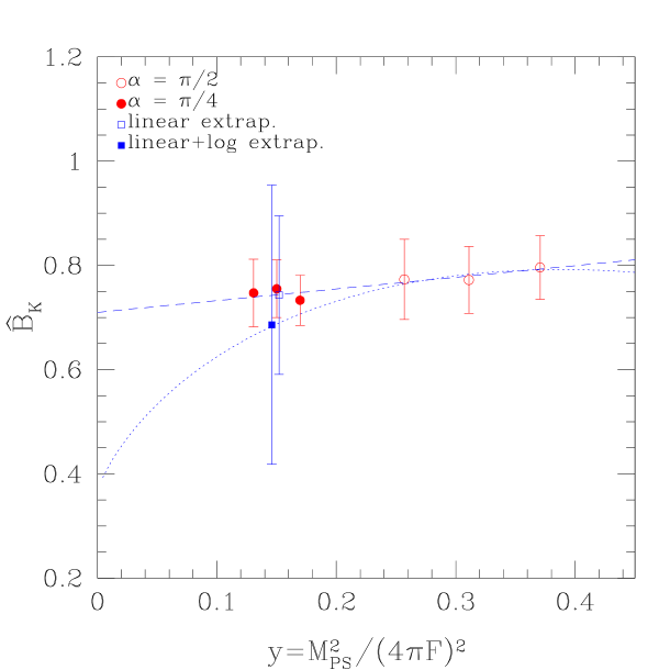
Figure 10: Linear vs. chiral log extrapolation of $\hat{B}_{K}$ to its physical mass value.

Next we perform both a linear extrapolation and one based on Eq. (C.97). The results of these two extrapolated $\hat{B}_{K}$ values are shown in Fig. 10, where they are compared to the continuum $\hat{B}_{K}$ estimates, obtained with the same procedure from the $\pi/4$ data, practically computed at the physical mass point. We see that, within large errors, the chiral logs are not resolved by our data. Nevertheless, it appears that the linear extrapolation performs somewhat better than the chiral log one.

A last interesting point concerns the comparison of our best $\hat{B}_{K}$ estimate (see Eq. (6.74)) to the one obtained in this Appendix, from the linear extrapolation:

$$\hat{B}_{K}=0.74\pm 0.15\,.$$ (C.98)

The difference in the extraction of the two results is essentially that the extrapolations in the mass and the continuum limit have been swapped . The fact that the two results are compatible means that, for the mass ranges under consideration, the order in which these limits are taken is irrelevant. This is clearly not true close to the chiral limit.

D Exceptional configurations

The initial motivation behind the introduction of tmQCD was the problem of exceptional configurations [51], which is solved by cutting-off in the IR limit the low-lying eigenvalues of the lattice Dirac operator, with the twisted mass $\mu_{l}$ [12]. The tmQCD action we have adopted so far refers to the light flavours, whereas the strange quark propagator, being regularised by the standard Wilson fermion action, is not immune from exceptional configurations. The common lore [23] is that for the values of $\kappa_{s}$ of Table 1 (corresponding to a $K$-meson of more than $600~{}{\rm MeV}$), no exceptional configurations ought to occur. In fact, none of the runs reported above showed any signs of such a problem.

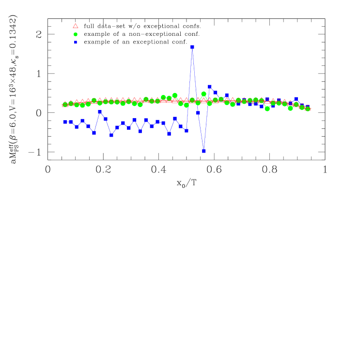
Figure 1: The value of $aM_{\rm PS}^{\rm eff}$ for: (i) an exceptional configuration; (ii) a typical configuration of our ensemble; (iii) the mean value, averaged on the configuration ensemble, without the exceptional configuration.

Nevertheless, evidence of an exceptional configuration showed up in an aside simulation, after 363 measurements at $\beta=6.0$, a $16^{3}\times 48$ lattice volume and $\kappa_{s}=0.1342$ (for the record we mention that in the run, $\kappa_{d}=0.135194$ and $a\mu_{d}=0.01051$). Thus the problem arose, somewhat surprisingly, at a $\kappa_{s}$ believed to be safe, on empirical grounds.

In this respect we have considered the effective mass $aM_{\rm PS}^{\rm eff}$, as obtained in standard (non-twisted) lattice QCD. This is like the quantity computed in Eq. (4.66), without the $f_{\rm V}$ correlation functions and with $f_{\rm A}$ made up of only standard (non-twisted) Wilson quarks (i.e. the strange flavours of our formulation). In Fig. 1 we plot $aM_{\rm PS}^{\rm eff}$, calculated at the exceptional configuration as well as at a typical configuration of our ensemble. These results are compared to the average $aM_{\rm PS}^{\rm eff}$, computed on the whole ensemble, save for the exceptional configuration. This plot is a clear warning against simulating even at reputedly safe values of the Wilson hopping parameter. We point out that several lattice measurements, besides our own, have been performed by other collaborations at this hopping parameter (e.g. see ref. [11]).

E Comparison with the $B_{K}$ computation of ref. [11]

In this Appendix we compare our results to the most recent ones obtained with Wilson fermions [11], where $\hat{B}_{K}=0.96\pm 0.10$ is quoted. There are a few similarities and several differences between the two approaches:

• In both approaches Wilson fermions are used, but in the present work we have a twisted term in the lattice action. In ref. [11] the $\Delta S=2$ bare matrix element is computed on periodic lattices, from a four-point correlation function of the operator $O_{\rm VA+AV}$ (which is related to the three-point correlation function of $O_{\rm VV+AA}$ through Ward identities). In the present work it is computed from a three-point correlation function of the operator $O_{\rm VA+AV}$ (which is related to the three-point correlation function of $O_{\rm VV+AA}$ through the tmQCD formalism). Schrödinger functional boundary conditions are used, which amounts to smeared pseudoscalar sources at the two time boundaries.

• In both approaches matrix elements are renormalised non-perturbatively. In ref. [11] the renormalisation constants are computed in the RI/MOM scheme, at scales of a few GeV. The RGI $\hat{B}_{K}$ requires also the operator RG-running; this is performed in NLO perturbation theory. In the present work, matrix elements are renormalised at hadronic scales in a SF scheme. The RG-running is performed non-perturbatively, using finite volume techniques, up to a few tens of GeV and subsequently with NLO perturbation theory.

• In the present work, $B_{K}$ is extracted directly from suitable ratios of correlation functions. In ref. [11], $B_{K}$ is obtained from the slope of the four-fermion operator matrix element, as a function of its vacuum saturation estimate $(8/3)F_{K}^{2}m_{K}^{2}$. This linear behaviour is predicted by lowest order chiral perturbation theory and is also seen in the data produced at pseudoscalar masses above the value of the physical $K$-meson mass.

It is interesting to try and understand the source of the difference in the $\hat{B}_{K}$ value quoted by us and by the authors of ref. [11]. First we compare the quantity $\mathcal{Z}_{\rm VA+AV;1}^{+}(g_{0})$ of ref. [13] to the same quantity, calculated in the the RI/MOM scheme; this is done by combining the $Z_{\rm VA+AV}$ values of ref. [52], used in the $B_{K}$ computation of ref. [11], with the NLO running quoted in refs. [2, 3]. The two estimates do not depend on the renormalisation scheme in which they have been computed. They only differ by (i) discretisation effects; (ii) the reliability (convergence) of the NLO perturbative running, calculated in two different schemes and applied at two different scales. In Fig. 11 we show the quantity

$$\Delta=\dfrac{\mathcal{Z}_{\rm VA+AV;1}^{+}-\mathcal{Z}_{\rm VA+AV;{\rm RI/MOM}}^{+}}{\mathcal{Z}_{\rm VA+AV;1}^{+}}$$ (E.99)

as a function of the lattice spacing. It is clear that a barely significant difference at the largest lattice spacing, quickly disappears as the continuum limit is approached. Thus it seems that renormalisation is not responsible for the different $\hat{B}_{K}$ results quoted by the two groups.

In order to have as direct a comparison as possible, we compute in the $\alpha=\pi/2$ case the quantity

$$\hat{R}^{\prime}=\dfrac{iZ_{\rm VA+AV}F_{\rm VA+AV}}{2[f_{\rm\scriptscriptstyle P}(x_{0})-i\dfrac{Z_{\rm S}}{Z_{\rm P}}f_{\rm\scriptscriptstyle S}(x_{0})][f_{\rm\scriptscriptstyle P}^{\prime}(T-x_{0})-i\dfrac{Z_{\rm S}}{Z_{\rm P}}f_{\rm\scriptscriptstyle S}^{\prime}(T-x_{0})]}\,.$$ (E.100)

The computation is performed at each value of the inverse coupling $\beta$ and mass parameters $\kappa_{s}$ and ($\kappa_{d},a\mu$) of Table 1. The normalisation factor $Z_{\rm S}/Z_{\rm P}=(ZZ_{\rm A})^{-1}$ is calculated from the $Z$ and $Z_{\rm A}$ ALPHA collaboration estimates quoted in Appendix A.

A glance at Eqs. (2.15,2.16, B.92,B.93) shows that the above ratio tends, at large time separations, to the quantity

$$\hat{R}^{\prime}\rightarrow\dfrac{Z_{\rm VA+AV}\langle\bar{K}^{0}|O_{\rm VA+AV}|K^{0}\rangle}{|\langle 0|P_{sd}|K^{0}\rangle|^{2}}\,.$$ (E.101)

Finally, for each set of coupling and mass parameter values, we construct the quantity

$$\hat{R}^{\prime}_{\rm RGI}=\mathcal{Z}_{\rm VA+AV;1}^{+}(g_{0})\,\,R^{\prime}$$ (E.102)

in exactly the same way we have computed $\hat{B}_{K}$ of eq. (6.72). This quantity may be directly compared to the ratio $\hat{R}^{\rm w/o\,\,\,subtr.}$ of ref. [11] (see Table 1 of that work; the same quantity is sometimes referred to as $R^{rgi}$ by the authors).

We also compute the quantity

$$X^{\prime}=\dfrac{8}{3}\dfrac{[Z_{\rm A}f_{\rm\scriptscriptstyle A}(x_{0})-iZ_{\rm V}f_{\rm\scriptscriptstyle V}(x_{0})][Z_{\rm A}f_{\rm\scriptscriptstyle P}^{\prime}(T-x_{0})-iZ_{\rm V}f_{\rm\scriptscriptstyle S}^{\prime}(T-x_{0})]}{[f_{\rm\scriptscriptstyle P}(x_{0})-i\dfrac{Z_{\rm S}}{Z_{\rm P}}f_{\rm\scriptscriptstyle S}(x_{0})][f_{\rm\scriptscriptstyle P}^{\prime}(T-x_{0})-i\dfrac{Z_{\rm S}}{Z_{\rm P}}f_{\rm\scriptscriptstyle S}^{\prime}(T-x_{0})]}\,.$$ (E.103)

This ratio tends, at large time separations, to the quantity

$$X^{\prime}\rightarrow\dfrac{8}{3}\dfrac{F_{K}^{2}m_{K}^{2}}{|\langle 0|P_{sd}|K^{0}\rangle|^{2}}\,,$$ (E.104)

which is the same quantity as $X$ of ref. [11]. For both $\hat{R}^{\prime}_{\rm RGI}$ and $X^{\prime}$ we have used ALPHA collaboration renormalisation constants.

At fixed gauge coupling $\beta$, the quantity $\hat{R}^{\prime}_{\rm RGI}$ is fit linearly as a function of $X^{\prime}$; the slope is the $\hat{B}_{K}$ estimate according to lowest order chiral perturbation theory. In Fig. 11 we compare the results of ref. [11] to our results (obtained as described here from the ratio $\hat{R}^{\prime}_{\rm RGI}$) and find them compatible. We also see that our preferred $B_{K}$ estimates (obtained on the same gauge configurations, but extracted from the ratio $R_{B}$) give a consistently lower $B_{K}$ estimate. This shows that the discrepancy of the two results is not due to different regularisation and renormalisation systematics, but due to the different method of extraction of $B_{K}$.

The errors we quote for the results of the present method are larger than those of ref. [11]. This is due to the fact that the latter results have been obtained, at fixed $\beta$ and for several values of the hopping parameters, on the same configuration ensemble, while we have generated a separate ensemble at each $\kappa$. Thus, the extrapolations in the pseudoscalar mass in ref. [11] benefit from the correlations between measurements. On the other hand, for both datasets, $\hat{B}_{K}$ has been computed from the slope of $\hat{R}^{\prime}_{\rm RGI}$ as a function of $X^{\prime}$. This fitting procedure enlarges the errors, as can be seen by comparing them to those of our main method (based upon computing $R_{B}$ at several $\kappa$-values and extrapolating it to the physical Kaon mass).

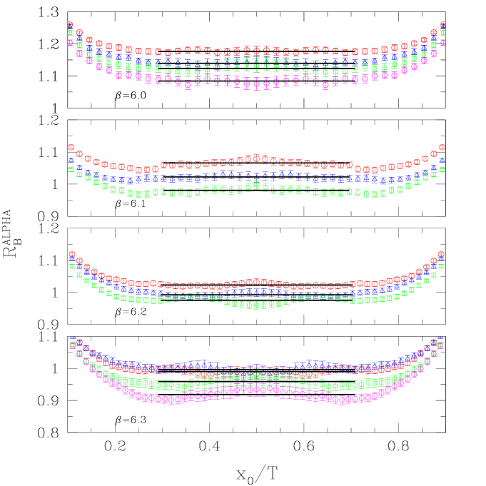
Figure 4: Plateaux for the extraction of $R_{\rm B}^{\rm ALPHA}$ at $\alpha=\pi/2$. The time-range and value of each plateau is indicated by a straight line segment.

Figure 6: Linear extrapolation of $R_{\rm B}$ to the physical kaon mass at $\alpha=\pi/2$.

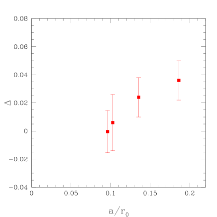
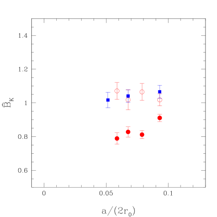
Figure 11: Top: $\Delta$ is the difference of $\mathcal{Z}_{\rm VA+AV;1}^{+}$, computed in the SF scheme [13] and $\mathcal{Z}_{\rm VA+AV;{\rm RI/MOM}}^{+}$, computed in the RI/MOM scheme [52], normalised by $\mathcal{Z}_{\rm VA+AV;1}^{+}$. It is a discretisation effect which vanishes close to the continuum limit. Bottom: Comparison of $\hat{B}_{K}$ obtained from three different methods: (i) results of ref. [11] (filled squares); (ii) results obtained from our data (tmQCD and SF-renormalisation), using the method of ref. [11] (open circles); (iii) the main results of the present work (filled circles).

References

- [1] A. Buras, “Weak Hamiltonian, CP-violation and Rare Decays”, Published in Les Houches 1997, “Probing the Standard Model of particle interactions”, eds. F. David and R. Gupta, Elsevier Science (1998) 281–539, [arXiv:hep-ph/9806471].
- [2] M. Ciuchini, E. Franco, V. Lubicz, G. Martinelli, I. Scimemi, and L. Silvestrini, “Next-to-leading order QCD corrections to effective Hamiltonians”, Nucl. Phys. B523 (1998) 501–525, [arXiv:hep-ph/9711402].
- [3] A. Buras, M. Misiak, and J. Urban, “Two loop QCD anomalous dimensions of flavor changing four quark operators within and beyond the Standard Model”, Nucl. Phys. B586 (2000) 397–426, [arXiv:hep-ph/0005183].
- [4] C. Dawson, “Progress in Kaon Phenomenology from Lattice QCD”, PoS LAT2005 (2005) 007.
- [5] G. Martinelli, “The four fermion operators of the weak Hamiltonian on the lattice and in the continuum”, Phys. Lett. B141 (1984) 395–399.
- [6] C. Bernard, T. Draper, and A. Soni, “Perturbative corrections to four fermion operators on the lattice”, Phys. Rev. D36 (1987) 3224–3244.
- [7] C. Bernard, T. Draper, G. Hockney, and A. Soni, “Recent developments in weak matrix element calculations”, Nucl. Phys. Proc. Suppl. 4 (1998) 483–492.
- [8] R. Gupta, D. Daniel, G. Kilcup, A. Patel, and S. S.R., “The Kaon B-parameter with Wilson fermions”, Phys. Rev. D47 (1993) 5113–5127, [arXiv:hep-lat/9210018].
- [9] A. Donini, V. Giménez, G. Martinelli, M. Talevi, and A. Vladikas, “Non-perturbative renormalization of lattice four-fermion operators without power subtractions”, Eur. Phys. J. C10 (1999) 121–142, [arXiv:hep-lat/9902030].
- [10] D. Bećirević, P. Boucaud, V. Giménez, V. Lubicz, G. Martinelli, J. Micheli, and M. Papinutto, “ - mixing with Wilson fermions without subtractions”, Phys. Lett. B487 (2000) 74–80, [arXiv:hep-lat/0005013].
- [11] D. Bećirević, P. Boucaud, V. Giménez, V. Lubicz, and M. Papinutto, “ from the lattice with Wilson quarks”, Eur. Phys. J. C37 (2004) 315–321, [arXiv:hep-lat/0407004].
- [12] ALPHA Collaboration, R. Frezzotti, P. A. Grassi, S. Sint, and P. Weisz, “Lattice QCD with a chirally twisted mass term”, JHEP 08 (2001) 058, [arXiv:hep-lat/0101001].
- [13] ALPHA Collaboration, M. Guagnelli, J. Heitger, C. Pena, S. Sint, and A. Vladikas, “Non-perturbative renormalization of left-left four-fermion operators in quenched lattice QCD”, arXiv:hep-lat/0505002.
- [14] ALPHA Collaboration, P. Dimopoulos, J. Heitger, C. Pena, S. Sint, and A. Vladikas, “ from twisted mass QCD”, Nucl. Phys. Proc. Suppl. 129 (2004) 308–310, [arXiv:hep-lat/0309134].
- [15] ALPHA Collaboration, P. Dimopoulos, J. Heitger, C. Pena, S. Sint, and A. Vladikas, “Precision computation of in quenched lattice QCD”, Nucl. Phys. Proc. Suppl. 140 (2005) 362–364, [arXiv:hep-lat/0409026].
- [16] M. Della Morte, “Wilson-like fermions and the static parameter with no chirality breaking mixings”, Nucl. Phys. Proc. Suppl. 140 (2005) 458–460, [arXiv:hep-lat/0409012].
- [17] F. Palombi, M. Papinutto, C. Pena, and H. Wittig, “ mixing in the static approximation from the Schrödinger functional and twisted mass QCD”, arXiv:hep-lat/0509008.
- [18] ALPHA Collaboration, C. Pena, S. Sint, and A. Vladikas, “Twisted mass QCD and lattice approaches to the rule”, JHEP 09 (2004) 069, [arXiv:hep-lat/0405028].
- [19] S. Sharpe, “Quenched chiral logarithms”, Phys.Rev. D46 (1992) 3146–3168, [arXiv:hep-lat/9205020].
- [20] S. Sharpe, “Phenomenology from the lattice”, Boulder TASI 45 (1994) 377–444, [arXiv:hep-lat/9412243].
- [21] S. Sharpe and Y. Zhang, “Quenched chiral perturbation theory for heavy-light mesons”, Phys.Rev. D53 (1996) 5125–5135, [arXiv:hep-lat/9510037].
- [22] M. Golterman and K. Leung, “Chiral perturbation theory for decay in the continuum and on the lattice”, Phys. Rev. D56 (1997) 2950–2969, [arXiv:hep-lat/9702015].
- [23] ALPHA & UKQCD Collaboration, J. Garden, J. Heitger, R. Sommer, and H. Wittig, “Precision computation of the strange quark’s mass in quenched QCD”, Nucl. Phys. B571 (2000) 237–256, [arXiv:hep-lat/9906013].
- [24] LF Collaboration, K. Jansen, C. McNeile, C. Michael, K. Nagai, M. Papinutto, J. Pickavance, A. Shindler, C. Urbach, and I. Wetzorke, “Flavour breaking effects of Wilson twisted mass fermions”, arXiv:hep-lat/0507032.
- [25] F. Farchioni, K. Jansen, C. McNeile, C. Michael, I. Montvay, K. Nagai, M. Papinutto, J. Pickavance, E. Scholz, L. Scorzato, A. Shindler, N. Ukita, C. Urbach, U. Wenger, and I. Wetzorke, “Twisted mass fermions: Neutral pion masses from disconnected contributions”, arXiv:hep-lat/0509036.
- [26] B. Sheikholeslami and R. Wohlert, “Improved continuum limit lattice action for QCD with Wilson fermions”, Nucl. Phys. B259 (1985) 572.
- [27] K. Jansen, C. Liu, M. Lüscher, H. Simma, S. Sint, R. Sommer, P. Weisz, and U. Wolff, “Nonperturbative renormalization of lattice QCD at all scales”, Phys. Lett. B372 (1996) 275–282, [arXiv:hep-lat/9512009].
- [28] M. Lüscher, S. Sint, R. Sommer, and P. Weisz, “Chiral symmetry and O() improvement in lattice QCD”, Nucl. Phys. B478 (1996) 365–400, [arXiv:hep-lat/9605038].
- [29] ALPHA Collaboration, R. Frezzotti, S. Sint, and P. Weisz, “O(a) improved twisted mass lattice QCD”, JHEP 07 (2001) 048, [arXiv:hep-lat/0104014].
- [30] R. Frezzotti and G. C. Rossi, “Chirally improving Wilson fermions. II: Four-quark operators”, JHEP 10 (2004) 070, [arXiv:hep-lat/0407002].
- [31] ALPHA Collaboration, M. Guagnelli, J. Heitger, R. Sommer, and H. Wittig, “Hadron masses and matrix elements from the QCD Schrödinger functional”, Nucl. Phys. B560 (1999) 465, [arXiv:hep-lat/9903040].
- [32] M. Lüscher, R. Narayanan, P. Weisz, and U. Wolff, “The Schrödinger functional: A Renormalizable probe for non-Abelian gauge theories”, Nucl. Phys. B384 (1992) 168–228, [arXiv:hep-lat/9207009].
- [33] S. Sint, “On the Schrödinger functional in QCD”, Nucl. Phys. B421 (1994) 135–158, [arXiv:hep-lat/9312079].
- [34] M. Lüscher and P. Weisz, “Definition and general properties of the transfer matrix in continuum limit improved lattice gauge theories”, Nucl. Phys. B240 (1984) 349.
- [35] M. Lüscher, “Construction of a Selfadjoint, Strictly Positive Transfer Matrix for Euclidean Lattice Gauge Theories”, Commun. math. Phys. 54 (1977) 283.
- [36] S. Sint, “The Schrödinger functional with chirally rotated boundary conditions”, PoS LAT2005 (2005) 235, [arXiv:hep-lat/0511034].
- [37] R. Sommer, “A New way to set the energy scale in lattice gauge theories and its applications to the static force and in SU(2) Yang-Mills theory”, Nucl. Phys. B411 (1994) 839, [arXiv:hep-lat/9310022].
- [38] M. Lüscher, S. Sint, R. Sommer, P. Weisz, and U. Wolff, “Non-perturbative O() improvement of lattice QCD”, Nucl. Phys. B491 (1997) 323–343, [arXiv:hep-lat/9609035].
- [39] M. Lüscher, S. Sint, R. Sommer, and H. Wittig, “Nonperturbative determination of the axial current normalization constant in O() improved lattice QCD”, Nucl. Phys. B491 (1997) 344–364, [arXiv:hep-lat/9611015].
- [40] T. Bhattacharya, R. Gupta, W.-J. Lee, and S. Sharpe, “O() improved renormalization constants”, Phys. Rev. D63 (2001) 074505, [arXiv:hep-lat/0009038].
- [41] T. Bhattacharya, R. Gupta, W.-J. Lee, and S. Sharpe, “Scaling behaviour of improvement and renormalization constants”, Nucl. Phys. Proc. Suppl. 106 (2002) 789–791, [arXiv:hep-lat/0111001].
- [42] T. Bhattacharya, R. Gupta, W. Lee, and S. Sharpe, “Scaling behavior of discretization errors in renormalization and improvement constants”, arXiv:hep-lat/0509160.
- [43] L. Giusti, P. Hernández, M. Laine, P. Weisz, and H. Wittig, “Low-energy couplings of QCD from current correlators near the chiral limit”, JHEP 04 (2004) 013, [arXiv:hep-lat/0402002].
- [44] ALPHA Collaboration, J. Rolf and S. Sint, “A precise determination of the charm quark’s mass in quenched QCD”, JHEP 12 (2002) 007, [arXiv:hep-ph/0209255].
- [45] ALPHA Collaboration, F. Palombi, , C. Pena, and S. Sint, “A perturbative study of two four-quark operators in finite volume renormalization schemes”, arXiv:hep-lat/0505003.
- [46] G. Altarelli, G. Curci, G. Martinelli, and S. Petrarca, “QCD nonleading corrections to weak decays as an application of regularization by dimensional reduction”, Nucl. Phys. B187 (1981) 461.
- [47] ALPHA Collaboration, S. Capitani, M. Lüscher, R. Sommer, and H. Wittig, “Nonperturbative quark mass renormalization in quenched lattice QCD”, Nucl. Phys. B544 (1999) 669, [arXiv:hep-lat/9810063].
- [48] ALPHA Collaboration, M. Guagnelli, R. Petronzio, J. Rolf, S. Sint, R. Sommer, and U. Wolff, “Non-perturbative results for the coefficients and in O() improved lattice QCD”, Nucl. Phys. B595 (2001) 44–62, [arXiv:hep-lat/0009021].
- [49] S. Sint and P. Weisz, “Further results on O() improved lattice QCD to one-loop order of perturbation theory”, Nucl. Phys. B502 (1997) 251–268, [arXiv:hep-lat/9704001].
- [50] S. Necco and R. Sommer, “The heavy quark potential from short to intermediate distances”, Nucl. Phys. B622 (2002) 328–346, [arXiv:hep-lat/0108008].
- [51] P. de Forcrand, K. H. Mütter, K. Schilling, and R. Sommer, “Towards the limit of the quenched approximation in hadron mass calculations”, Published in BNL Gauge Theor. Symp. 45 (1986) 257.
- [52] D. Bećirević, V. Giménez, V. Lubicz, G. Martinelli, M. Papinutto, and J. Reyes, “Renormalization constants of quark operators for the non-pertrubatively improved Wilson action”, JHEP 08 (2004) 022, [arXiv:hep-lat/0401033].