TASI 2004 Lecture Notes on Higgs Boson Physics

Abstract

In these lectures I briefly review the Higgs mechanism of spontaneous symmetry breaking and focus on the most relevant aspects of the phenomenology of the Standard Model and of the Minimal Supersymmetric Standard Model Higgs bosons at both hadron (Tevatron, Large Hadron Collider) and lepton (International Linear Collider) colliders. Some emphasis is put on the perturbative calculation of both Higgs boson branching ratios and production cross sections, including the most important radiative corrections.

I Introduction

The origin of the electroweak symmetry breaking is among the most important open questions of contemporary particle physics. Since it was first proposed in 1964 by Higgs, Kibble, Guralnik, Hagen, Englert, and Brout Englert:1964et ; Higgs:1964pj ; Guralnik:1964eu , the mechanism of spontaneous symmetry breaking known as Higgs mechanism has become part of the Standard Model (SM) of particle physics and of one of its most thoroughly studied extensions, the Minimal Supersymmetric Standard Model (MSSM). A substantial theoretical and experimental effort has been devoted to the study of the physics of the single scalar Higgs boson predicted by the realization of the Higgs mechanism in the SM, and of the multiple scalar and pseudoscalar Higgs bosons arising in the MSSM. Indeed, the discovery of one or more Higgs bosons is among the most important goals of both the Tevatron and the Large Hadron Collider (LHC), while the precise determination of their physical properties strongly support the need for a future high energy International Linear Collider (ILC).

In these lectures I would like to present a self contained introduction to the physics of the Higgs boson(s). Given the huge amount of work that has been done in this field, I will not even come close to being exhaustively complete. This is not actually my aim. For this series of lectures, I would like to present the reader with some important background of informations that could prepare her or him to explore further topical issues in Higgs physics. Also, alternative theoretical approaches to the electroweak symmetry breaking and the generation of both boson and fermion masses will not be considered here. They have been covered in several other series of lectures at this school, and to them I refer.

In Section II, after a brief glance at the essence of the Higgs mechanism, I will review how it is embedded in the Standard Model and what constraints are directly and indirectly imposed on the mass of the single Higgs boson that is predicted in this context. Among the extensions of the SM I will only consider the case of the MSSM, and in this context I will mainly focus on those aspects that could be more relevant to distinguish the MSSM Higgs bosons. Section III will review the phenomenology of both the SM and the MSSM Higgs bosons, at the Tevatron and the LHC, and will then focus on the role that a high energy ILC could play in this context. Finally, in Section IV, I will briefly summarize the state of the art of existing theoretical calculations for both decay rates and production cross sections of a Higgs boson.

Let me conclude by pointing the reader to some selected references available in the literature. The theoretical bases of the Higgs mechanism are nowadays a matter for textbooks in Quantum Field Theory. They are presented in depth in both Refs. Peskin:1995ev and Weinberg:1995mt . An excellent review of both SM and MSSM Higgs physics, containing a very comprehensive discussion of both theoretical and phenomenological aspects as well as an exhaustive bibliography, has recently appeared Djouadi:2005gi ; Djouadi:2005gj . The phenomenology of Higgs physics has also been thoroughly covered in a fairly recent review paper Carena:2002es , which can be complemented by several workshop proceedings and reports cms:1994tdr ; atlas:1999tdr ; Carena:2000yx ; Cavalli:2002vs ; Babukhadia:2003zu ; Assamagan:2004mu ; Abe:2001wn ; Aguilar-Saavedra:2001rg . Finally, series of lectures given at previous summer schools Dawson:1994ri ; Dawson:1998yi can provide excellent references.

II Theoretical framework: the Higgs mechanism and its consequences.

In Yang-Mills theories gauge invariance forbids to have an explicit mass term for the gauge vector bosons in the Lagrangian. If this is acceptable for theories like QED (Quantum Electrodynamics) and QCD (Quantum Chromodynamics), where both photons and gluons are massless, it is unacceptable for the gauge theory of weak interactions, since both the charged ($W^{\pm}$) and neutral ($Z^{0}$) gauge bosons have very heavy masses ($M_{W}\!\simeq\!80$ GeV, $M_{Z}\!\simeq\!91$ GeV). A possible solution to this problem, inspired by similar phenomena happening in the study of spin systems, was proposed by several physicists in 1964 Englert:1964et ; Higgs:1964pj ; Guralnik:1964eu , and it is known today simply as the Higgs mechanism. We will review the basic idea behind it in Section II.1. In Section II.2 we will recall how the Higgs mechanism is implemented in the Standard Model and we will discuss which kind of theoretical constraints are imposed on the Higgs boson, the only physical scalar particle predicted by the model. Finally, in Section II.4 we will generalize our discussion to the case of the MSSM, and use its extended Higgs sector to illustrate how differently the Higgs mechanism can be implemented in extensions of the SM.

II.1 A brief introduction to the Higgs mechanism

The essence of the Higgs mechanism can be very easily illustrated considering the case of a classical abelian Yang-Mills theory. In this case, it is realized by adding to the Yang-Mills Lagrangian

$$\mathcal{L}_{A}=-\frac{1}{4}F^{\mu\nu}F_{\mu\nu}\,\,\,\,\,\,\mbox{with}\,\,\,\,\,\,F^{\mu\nu}=(\partial^{\mu}A^{\nu}-\partial^{\nu}A^{\mu})\,\,\,,$$ (1)

a complex scalar field with Lagrangian

$$\mathcal{L}_{\phi}=(D^{\mu}\phi)^{\ast}D_{\mu}\phi-V(\phi)=(D^{\mu}\phi)^{\ast}D_{\mu}\phi-\mu^{2}\phi^{\ast}\phi-\lambda(\phi^{\ast}\phi)^{2}\,\,\,,$$ (2)

where $D^{\mu}\!=\!\partial^{\mu}+igA^{\mu}$, and $\lambda\!>\!0$ for the scalar potential to be bounded from below. The full Lagrangian

$$\mathcal{L}=\mathcal{L}_{A}+\mathcal{L}_{\phi}$$ (3)

is invariant under a $U(1)$ gauge transformation acting on the fields as:

$$\phi(x)\rightarrow e^{i\alpha(x)}\phi(x)\,\,\,,\,\,\,A^{\mu}(x)\rightarrow A^{\mu}(x)+\frac{1}{g}\partial^{\mu}\alpha(x)\,\,\,,$$ (4)

while a gauge field mass term (i.e., a term quadratic in the fields $A^{\mu}$) would not be gauge invariant and cannot be added to $\mathcal{L}$ if the $U(1)$ gauge symmetry has to be preserved. Indeed, the Lagrangian in Eq. (3) can still describe the physics of a massive gauge boson, provided the potential $V(\phi)$ develops a non trivial minimum ($\phi^{\ast}\phi\!\neq\!0$). The occurrence of a non trivial minimum, or, better, of a non trivial degeneracy of minima only depends on the sign of the $\mu^{2}$ parameter in $V(\phi)$. For $\mu^{2}\!>\!0$ there is a unique minimum at $\phi^{\ast}\phi\!=\!0$, while for $\mu^{2}\!<\!0$ the potential develops a degeneracy of minima satisfying the equation $\phi^{\ast}\phi\!=\!-\mu^{2}/(2\lambda)$. This is illustrated in Fig. 1, where the potential $V(\phi)$ is plotted as a function of the real and imaginary parts of the field $\phi\!=\!\phi_{1}+i\phi_{2}$.

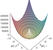
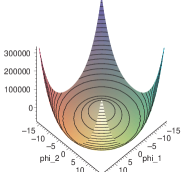
Figure 1: The potential $V(\phi)$ ($\phi\!=\phi_{1}+i\phi_{2}$) plotted for an arbitrary positive value of $\lambda$ and for an arbitrary positive (right) or negative (left) value of $\mu^{2}$.

In the case of a unique minimum at $\phi^{\ast}\phi\!=\!0$ the Lagrangian in Eq. (3) describes the physics of a massless vector boson (e.g. the photon, in electrodynamics, with $g\!=\!-e$) interacting with a massive charged scalar particle. On the other hand, something completely different takes place when $\mu^{2}\!<\!0$. Choosing the ground state of the theory to be a particular $\phi$ among the many satisfying the equation of the minimum, and expanding the potential in the vicinity of the chosen minimum, transforms the Lagrangian in such a way that the original gauge symmetry is now hidden or spontaneously broken, and new interesting features emerge. To be more specific, let’s pick the following $\phi_{0}$ minimum (along the direction of the real part of $\phi$, as traditional) and shift the $\phi$ field accordingly:

$$\phi_{0}=\left(-\frac{\mu^{2}}{2\lambda}\right)^{1/2}=\frac{v}{\sqrt{2}}\,\,\,\longrightarrow\,\,\,\phi(x)=\phi_{0}+\frac{1}{\sqrt{2}}\left(\phi_{1}(x)+i\phi_{2}(x)\right)\,\,\,.$$ (5)

The Lagrangian in Eq. (3) can then be rearranged as follows:

$${\mathcal{L}}=\underbrace{-\frac{1}{4}F^{\mu\nu}F_{\mu\nu}+\frac{1}{2}g^{2}v^{2}A^{\mu}A_{\mu}}_{\mathrm{massive}\,\,\mathrm{vector}\,\,\mathrm{field}}+\underbrace{\frac{1}{2}(\partial^{\mu}\phi_{1})^{2}+\mu^{2}\phi_{1}^{2}}_{\mathrm{massive}\,\,\mathrm{scalar}\,\,\mathrm{field}}+\underbrace{\frac{1}{2}(\partial^{\mu}\phi_{2})^{2}+gvA_{\mu}\partial^{\mu}\phi_{2}}_{\mathrm{Goldstone}\,\,\mathrm{boson}}+\ldots$$ (6)

and now contains the correct terms to describe a massive vector field $A^{\mu}$ with mass $m_{A}^{2}\!=\!g^{2}v^{2}$ (originating from the kinetic term of $\mathcal{L}_{\phi}$), a massive real scalar field $\phi_{1}$ with mass $m_{\phi_{1}}\!=\!-2\mu^{2}$, that will become a Higgs boson, and a massless scalar field $\phi_{2}$, a so called Goldstone boson which couples to the gauge vector boson $A^{\mu}$. The terms omitted contain couplings between the $\phi_{1}$ and $\phi_{2}$ fields irrelevant to this discussion. The gauge symmetry of the theory allows us to make the particle content more transparent. Indeed, if we parameterize the complex scalar field $\phi$ as:

$$\phi(x)=\frac{e^{i\frac{\chi(x)}{v}}}{\sqrt{2}}(v+H(x))\,\,\,\,\stackrel{{\scriptstyle U(1)}}{{\longrightarrow}}\,\,\,\,\frac{1}{\sqrt{2}}(v+H(x))\,\,\,,$$ (7)

the $\chi$ degree of freedom can be rotated away, as indicated in Eq. (7), by enforcing the $U(1)$ gauge invariance of the original Lagrangian. With this gauge choice, known as unitary gauge or unitarity gauge, the Lagrangian becomes:

$$\mathcal{L}=\mathcal{L}_{A}+\frac{g^{2}v^{2}}{2}A^{\mu}A_{\mu}+\frac{1}{2}\left(\partial^{\mu}H\partial_{\mu}H+2\mu^{2}H^{2}\right)+\ldots$$ (8)

which unambiguously describes the dynamics of a massive vector boson $A^{\mu}$ of mass $m_{A}^{2}\!=\!g^{2}v^{2}$, and a massive real scalar field of mass $m_{H}^{2}\!=\!-2\mu^{2}=2\lambda v^{2}$, the Higgs field. It is interesting to note that the total counting of degrees of freedom (d.o.f.) before the original $U(1)$ symmetry is spontaneously broken and after the breaking has occurred is the same. Indeed, one goes from a theory with one massless vector field (two d.o.f.) and one complex scalar field (two d.o.f.) to a theory with one massive vector field (three d.o.f.) and one real scalar field (one d.o.f.), for a total of four d.o.f. in both cases. This is what is colorfully described by saying that each gauge boson has eaten up one scalar degree of freedom, becoming massive.

We can now easily generalize the previous discussion to the case of a non-abelian Yang-Mills theory. $\mathcal{L}_{A}$ in Eq. (3) now becomes:

$$\mathcal{L}_{A}=\frac{1}{4}F^{a,\mu\nu}F^{a}_{\mu\nu}\,\,\,\,\,\mbox{with}\,\,\,\,\,F^{a}_{\mu\nu}=\partial_{\mu}A^{a}_{\nu}-\partial_{\nu}A^{a}_{\mu}+gf^{abc}A^{b}_{\mu}A^{c}_{\nu}\,\,\,,$$ (9)

where the latin indices are group indices and $f^{abc}$ are the structure constants of the Lie Algebra associated to the non abelian gauge symmetry Lie group, defined by the commutation relations of the Lie Algebra generators $t^{a}$: $[t^{a},t^{b}]\!=\!if^{abc}t^{c}$. Let us also generalize the scalar Lagrangian to include several scalar fields $\phi_{i}$ which we will in full generality consider as real:

$$\mathcal{L}_{\phi}=\frac{1}{2}(D^{\mu}\phi_{i})^{2}-V(\phi)\,\,\,\,\,\mbox{where}\,\,\,\,\,V(\phi)=\mu^{2}\phi_{i}^{2}+\frac{\lambda}{2}\phi_{i}^{4}\,\,\,,$$ (10)

where the sum over the index $i$ is understood and $D_{\mu}\!=\!\partial_{\mu}-igt^{a}A^{a}_{\mu}$. The Lagrangian of Eq. (3) is invariant under a non-abelian gauge transformation of the form:

$$\phi_{i}(x) \rightarrow (1+i\alpha^{a}(x)t^{a})_{ij}\phi_{j}\,\,\,,$$ (11)

$$A^{a}_{\mu}(x) \rightarrow A^{a}_{\mu}(x)+\frac{1}{g}\partial_{\mu}\alpha^{a}(x)+f^{abc}A^{b}_{\mu}(x)\alpha^{c}(x)\,\,\,.$$

When $\mu^{2}\!<\!0$ the potential develops a degeneracy of minima described by the minimum condition: $\phi^{2}\!=\!\phi_{0}^{2}\!=\!-\mu^{2}/\lambda$, which only fixes the magnitude of the vector $\phi_{0}$. By arbitrarily choosing the direction of $\phi_{0}$, the degeneracy is removed. The Lagrangian can be expanded in a neighborhood of the chosen minimum and mass terms for the gauge vector bosons can be introduced as in the abelian case, i.e.:

$$\frac{1}{2}(D_{\mu}\phi_{i})^{2} \longrightarrow \ldots\,\,\,+\frac{1}{2}g^{2}(t^{a}\phi)_{i}(t^{b}\phi)_{i}A_{\mu}^{a}A^{b\mu}+\ldots$$

$$\stackrel{{\scriptstyle\phi_{min}\!=\!\phi_{0}}}{{\longrightarrow}} \ldots\,\,\,+\frac{1}{2}\underbrace{g^{2}(t^{a}\phi_{0})_{i}(t^{b}\phi_{0})_{i}}_{m_{ab}^{2}}A_{\mu}^{a}A^{b\mu}+\ldots$$

Upon diagonalization of the mass matrix $m_{ab}^{2}$ in Eq. (II.1), all gauge vector bosons $A_{\mu}^{a}$ for which $t^{a}\phi_{0}\neq 0$ become massive, and to each of them corresponds a Goldstone particle, i.e. an unphysical massless particle like the $\chi$ field of the abelian example. The remaining scalar degrees of freedom become massive, and correspond to the Higgs field $H$ of the abelian example.

The Higgs mechanism can be very elegantly generalized to the case of a quantum field theory when the theory is quantized via the path integral method. In this context, the quantum analog of the potential $V(\phi)$ is the effective potential $V_{eff}(\varphi_{cl})$, defined in term of the effective action $\Gamma[\phi_{cl}]$ (the generating functional of the 1PI connected correlation functions) as:

$$V_{eff}(\varphi_{cl})=-\frac{1}{VT}\Gamma[\phi_{cl}]\,\,\,\,\,\mbox{for}\,\,\,\,\,\phi_{cl}(x)=\mbox{constant}=\varphi_{cl}\,\,\,,$$ (13)

where $VT$ is the space-time extent of the functional integration and $\phi_{cl}(x)$ is the vacuum expectation value of the field configuration $\phi(x)$:

$$\phi_{cl}(x)=\langle\Omega|\phi(x)|\Omega\rangle\,\,\,.$$ (14)

The stable quantum states of the theory are defined by the variational condition:

$$\frac{\delta}{\delta\phi_{cl}}\Gamma[\phi_{cl}]\bigg{|}_{\phi_{cl}=\varphi_{cl}}=0\,\,\,\,\,\,\,\,\longrightarrow\,\,\,\,\,\,\,\,\frac{\partial}{\partial\varphi_{cl}}V_{eff}(\varphi_{cl})=0\,\,\,,$$ (15)

which identifies in particular the states of minimum energy of the theory, i.e. the stable vacuum states. A system with spontaneous symmetry breaking has several minima, all with the same energy. Specifying one of them, as in the classical case, breaks the original symmetry on the vacuum. The relation between the classical and quantum case is made even more transparent by the perturbative form of the effective potential. Indeed, $V_{eff}(\varphi_{cl})$ can be organized as a loop expansion and calculated systematically order by order in $\hbar$:

$$V_{eff}(\varphi_{cl})=V(\varphi_{cl})+\mbox{loop effects}\,\,\,,$$ (16)

with the lowest order being the classical potential in Eq. (2). Quantum corrections to $V_{eff}(\varphi_{cl})$ affect some of the properties of the potential and therefore have to be taken into account in more sophisticated studies of the Higgs mechanism for a spontaneously broken quantum gauge theory. We will see how this can be important in Section II.3 when we discuss how the mass of the SM Higgs boson is related to the energy scale at which we expect new physics effect to become relevant in the SM.

Finally, let us observe that at the quantum level the choice of gauge becomes a delicate issue. For example, in the unitarity gauge of Eq. (7) the particle content of the theory becomes transparent but the propagator of a massive vector field $A^{\mu}$ turns out to be:

$$\Pi^{\mu\nu}(k)=-\frac{i}{k^{2}-m_{A}^{2}}\left(g^{\mu\nu}-\frac{k^{\mu}k^{\nu}}{m_{A}^{2}}\right)\,\,\,,$$ (17)

and has a problematic ultra-violet behavior, which makes more difficult to consistently define and calculate ultraviolet-stable scattering amplitudes and cross sections. Indeed, for the very purpose of studying the renormalizability of quantum field theories with spontaneous symmetry breaking, the so called renormalizable or renormalizability gauges ($R_{\xi}$ gauges) are introduced. If we consider the abelian Yang-Mills theory of Eqs. (1)-(3), the renormalizable gauge choice is implemented by quantizing with a gauge condition $G$ of the form:

$$G=\frac{1}{\sqrt{\xi}}(\partial_{\mu}A^{\mu}+\xi gv\phi_{2})\,\,\,,$$ (18)

in the generating functional

$$Z[J]=C\int DA\,D\phi_{1}\,D\phi_{2}\exp\left[i\int(\mathcal{L}-\frac{1}{2}G^{2})\right]\mbox{det}\left(\frac{\delta G}{\delta\alpha}\right)\,\,\,,$$ (19)

where C is an overall factor independent of the fields, $\xi$ is an arbitrary parameter, and $\alpha$ is the gauge transformation parameter in Eq. (4). After having reduced the determinant in Eq. (19) to an integration over ghost fields ($c$ and $\bar{c}$), the gauge plus scalar fields Lagrangian looks like:

$$\mathcal{L}-\frac{1}{2}G^{2}+\mathcal{L}_{ghost} = -\frac{1}{2}A_{\mu}\left(-g^{\mu\nu}\partial^{2}+\left(1-\frac{1}{\xi}\right)\partial^{\mu}\partial^{\nu}-(gv)^{2}g^{\mu\nu}\right)A_{\nu}$$ (20)

$$+ \frac{1}{2}(\partial_{\mu}\phi_{1})^{2}-\frac{1}{2}m_{\phi_{1}}^{2}\phi_{1}^{2}+\frac{1}{2}(\partial_{\mu}\phi_{2})^{2}-\frac{\xi}{2}(gv)^{2}\phi_{2}^{2}+\cdots$$

$$+ \bar{c}\left[-\partial^{2}-\xi(gv)^{2}\left(1+\frac{\phi_{1}}{v}\right)\right]c\,\,\,,$$

such that:

$$\langle A^{\mu}(k)A^{\nu}(-k)\rangle = \frac{-i}{k^{2}-m_{A}^{2}}\left(g^{\mu\nu}-\frac{k^{\mu}k^{\nu}}{k^{2}}\right)+\frac{-i\xi}{k^{2}-\xi m_{A}^{2}}\left(\frac{k^{\mu}k^{\nu}}{k^{2}}\right)\,\,\,,$$

$$\langle\phi_{1}(k)\phi_{1}(-k)\rangle = \frac{-i}{k^{2}-m_{\phi_{1}}^{2}}\,\,\,,$$ (21)

$$\langle\phi_{2}(k)\phi_{2}(-k)\rangle = \langle c(k)\bar{c}(-k)\rangle=\frac{-i}{k^{2}-\xi m_{A}^{2}}\,\,\,,$$

where the vector field propagator has now a safe ultraviolet behavior. Moreover we notice that the $\phi_{2}$ propagator has the same denominator of the longitudinal component of the gauge vector boson propagator. This shows in a more formal way the relation between the $\phi_{2}$ degree of freedom and the longitudinal component of the massive vector field $A^{\mu}$, upon spontaneous symmetry breaking.

II.2 The Higgs sector of the Standard Model

The Standard Model is a spontaneously broken Yang-Mills theory based on the $SU(2)_{L}\times U(1)_{Y}$ non-abelian symmetry groupPeskin:1995ev ; Weinberg:1995mt . The Higgs mechanism is implemented in the Standard Model by introducing a complex scalar field $\phi$, doublet of $SU(2)$ with hypercharge $Y_{\phi}=1/2$,

$$\phi=\left(\begin{array}[]{c}\phi^{+}\\ \phi^{0}\end{array}\right)\,\,\,,$$ (22)

with Lagrangian

$$\mathcal{L}_{\phi}=(D^{\mu}\phi)^{\dagger}D_{\mu}\phi-\mu^{2}\phi^{\dagger}\phi-\lambda(\phi^{\dagger}\phi)^{2}\,\,\,,$$ (23)

where $D_{\mu}\phi=(\partial_{\mu}-igA^{a}_{\mu}\tau^{a}-ig^{\prime}Y_{\phi}B_{\mu})$, and $\tau^{a}\!=\!\sigma^{a}/2$ (for $a\!=\!1,2,3$) are the $SU(2)$ Lie Algebra generators, proportional to the Pauli matrix $\sigma^{a}$. The gauge symmetry of the Lagrangian is broken to $U(1)_{em}$ when a particular vacuum expectation value is chosen, e.g.:

$$\langle\phi\rangle=\frac{1}{\sqrt{2}}\left(\begin{array}[]{c}0\\ v\end{array}\right)\,\,\,\,\,\,\mbox{with}\,\,\,\,\,\,v=\left(\frac{-\mu^{2}}{\lambda}\right)^{1/2}\,\,\,\,\,(\mu^{2}<0,\,\lambda>0)\,\,\,.$$ (24)

Upon spontaneous symmetry breaking the kinetic term in Eq. (23) gives origin to the SM gauge boson mass terms. Indeed, specializing Eq. (II.1) to the present case, and using Eq. (24), one gets:

$$(D^{\mu}\phi)^{\dagger}D_{\mu}\phi \longrightarrow \cdots+\frac{1}{8}(0\,\,\,v)\left(gA_{\mu}^{a}\sigma^{a}+g^{\prime}B_{\mu}\right)\left(gA^{b\mu}\sigma^{b}+g^{\prime}B^{\mu}\right)\left(\begin{array}[]{c}0\\ v\end{array}\right)+\cdots$$

$$\longrightarrow \cdots+\frac{1}{2}\frac{v^{2}}{4}\left[g^{2}(A_{\mu}^{1})^{2}+g^{2}(A_{\mu}^{2})^{2}+(-gA_{\mu}^{3}+g^{\prime}B_{\mu})^{2}\right]+\cdots$$

One recognizes in Eq. (II.2) the mass terms for the charged gauge bosons $W^{\pm}_{\mu}$:

$$W^{\pm}_{\mu}=\frac{1}{\sqrt{2}}(A_{\mu}^{1}\pm A_{\mu}^{2})\,\,\,\,\longrightarrow\,\,\,\,M_{W}=g\frac{v}{2}\,\,\,,$$ (29)

and for the neutral gauge boson $Z^{0}_{\mu}$:

$$Z^{0}_{\mu}=\frac{1}{\sqrt{g^{2}+g^{\prime 2}}}(gA_{\mu}^{3}-g^{\prime}B_{\mu})\,\,\,\,\longrightarrow\,\,\,\,M_{Z}=\sqrt{g^{2}+g^{\prime 2}}\frac{v}{2}\,\,\,,$$ (30)

while the orthogonal linear combination of $A^{3}_{\mu}$ and $B_{\mu}$ remains massless and corresponds to the photon field ($A_{\mu}$):

$$A_{\mu}=\frac{1}{\sqrt{g^{2}+g^{\prime 2}}}(g^{\prime}A_{\mu}^{3}+gB_{\mu})\,\,\,\,\longrightarrow\,\,\,\,M_{A}=0\,\,\,,$$ (31)

the gauge boson of the residual $U(1)_{em}$ gauge symmetry.

The content of the scalar sector of the theory becomes more transparent if one works in the unitary gauge and eliminate the unphysical degrees of freedom using gauge invariance. In analogy to what we wrote for the abelian case in Eq. (7), this amounts to parametrize and rotate the $\phi(x)$ complex scalar field as follows:

$$\phi(x)=\frac{e^{\frac{i}{v}\vec{\chi}(x)\cdot\vec{\tau}}}{\sqrt{2}}\left(\begin{array}[]{c}0\\ v+H(x)\end{array}\right)\,\,\,\stackrel{{\scriptstyle SU(2)}}{{\longrightarrow}}\,\,\,\phi(x)=\frac{1}{\sqrt{2}}\left(\begin{array}[]{c}0\\ v+H(x)\end{array}\right)\,\,\,,$$ (32)

after which the scalar potential in Eq. (23) becomes:

$$\mathcal{L}_{\phi}=\mu^{2}H^{2}-\lambda vH^{3}-\frac{1}{4}H^{4}=-\frac{1}{2}M_{H}^{2}H^{2}-\sqrt{\frac{\lambda}{2}}M_{H}H^{3}-\frac{1}{4}\lambda H^{4}\,\,\,.$$ (33)

Three degrees of freedom, the $\chi^{a}(x)$ Goldstone bosons, have been reabsorbed into the longitudinal components of the $W^{\pm}_{\mu}$ and $Z^{0}_{\mu}$ weak gauge bosons. One real scalar field remains, the Higgs boson $H$, with mass $M_{H}^{2}\!=\!-2\mu^{2}=2\lambda v^{2}$ and self-couplings:

$=-3i\frac{M_{H}^{2}}{v}$

$=-3i\frac{M_{H}^{2}}{v^{2}}$

Furthermore, some of the terms that we omitted in Eq. (II.2), the terms linear in the gauge bosons $W^{\pm}_{\mu}$ and $Z^{0}_{\mu}$, define the coupling of the SM Higgs boson to the weak gauge fields:

$=2i\frac{M_{V}^{2}}{v}g^{\mu\nu}$

$=2i\frac{M_{V}^{2}}{v^{2}}g^{\mu\nu}$

We notice that the couplings of the Higgs boson to the gauge fields are proportional to their mass. Therefore $H$ does not couple to the photon at tree level. It is important, however, to observe that couplings that are absent at tree level may be induced at higher order in the gauge couplings by loop corrections. Particularly relevant to the SM Higgs boson phenomenology that will be discussed in Section III are the couplings of the SM Higgs boson to pairs of photons, and to a photon and a $Z^{0}_{\mu}$ weak boson:

as well as the coupling to pairs of gluons, when the SM Lagrangian is extended through the QCD Lagrangian to include also the strong interactions:

The analytical expressions for the $H\gamma\gamma$, $H\gamma Z$, and $Hgg$ one-loop vertices are more involved and will be given in Section III.1. As far as the Higgs boson tree level couplings go, we observe that they are all expressed in terms of just two parameters, either $\lambda$ and $\mu$ appearing in the scalar potential of $\mathcal{L}_{\phi}$ (see Eq. 23)) or, equivalently, $M_{H}$ and $v$, the Higgs boson mass and the scalar field vacuum expectation value. Since $v$ is measured in muon decay to be $v\!=\!(\sqrt{2}G_{F})^{-1/2}\!=\!246$ GeV, the physics of the SM Higgs boson is actually just function of its mass $M_{H}$.

The Standard Model gauge symmetry also forbids explicit mass terms for the fermionic degrees of freedom of the Lagrangian. The fermion mass terms are then generated via gauge invariant renormalizable Yukawa couplings to the scalar field $\phi$:

$$\mathcal{L}_{\mathit{Yukawa}}=-\Gamma_{u}^{ij}\bar{Q}^{i}_{L}\phi^{c}u^{j}_{R}-\Gamma_{d}^{ij}\bar{Q}^{i}_{L}\phi d^{j}_{R}-\Gamma_{e}^{ij}\bar{L}^{i}_{L}\phi l^{j}_{R}+h.c.$$ (34)

where $\phi^{c}\!=\!-i\sigma^{2}\phi^{\star}$, and $\Gamma_{f}$ ($f=u,d,l$) are matrices of couplings arbitrarily introduced to realize the Yukawa coupling between the field $\phi$ and the fermionic fields of the SM. $Q_{L}^{i}$ and $L_{L}^{i}$ (where $i=1,2,3$ is a generation index) represent quark and lepton left handed doublets of $SU(2)_{L}$, while $u_{R}^{i}$, $d_{R}^{i}$ and $l_{R}^{i}$ are the corresponding right handed singlets. When the scalar fields $\phi$ acquires a non zero vacuum expectation value through spontaneous symmetry breaking, each fermionic degree of freedom coupled to $\phi$ develops a mass term with mass parameter

$$m_{f}=\Gamma_{f}\frac{v}{\sqrt{2}}\,\,\,,$$ (35)

where the process of diagonalization from the current eigenstates in Eq. (34) to the corresponding mass eigenstates is understood, and $\Gamma_{f}$ are therefore the elements of the diagonalized Yukawa matrices corresponding to a given fermion $f$. The Yukawa couplings of the $f$ fermion to the Higgs boson ($y_{f}$) is proportional to $\Gamma_{f}$:

$=-i\frac{m_{f}}{v}=-i\frac{\Gamma_{f}}{\sqrt{2}}=-iy_{f}$

As long as the origin of fermion masses is not better understood in some more general context beyond the Standard Model, the Yukawa couplings $y_{f}$ represent free parameter of the SM Lagrangian. The mechanism through which fermion masses are generated in the Standard Model, although related to the mechanism of spontaneous symmetry breaking, requires therefore further assumptions and involves a larger degree of arbitrariness as compared to the gauge boson sector of the theory.

II.3 Theoretical constraints on the Standard Model Higgs boson mass

Several issues arising in the scalar sector of the Standard Model link the mass of the Higgs boson to the energy scale where the validity of the Standard Model is expected to fail. Below that scale, the Standard Model is the extremely successful effective field theory that emerges from the electroweak precision tests of the last decades. Above that scale, the Standard Model has to be embedded into some more general theory that gives origin to a wealth of new physics phenomena. From this point of view, the Higgs sector of the Standard Model contains actually two parameters, the Higgs mass ($M_{H}$) and the scale of new physics ($\Lambda$).

In this Section we will review the most important theoretical constraints that are imposed on the mass of the Standard Model Higgs boson by the consistency of the theory up to a given energy scale $\Lambda$. In particular we will touch on issues of unitarity, triviality, vacuum stability, fine tuning and, finally, electroweak precision measurements.

II.3.1 Unitarity

The scattering amplitudes for longitudinal gauge bosons ($V_{L}V_{L}\rightarrow V_{L}V_{L}$, where $V=W^{\pm},Z^{0}$) grow as the square of the Higgs boson mass. This is easy to calculate using the electroweak equivalence theorem Peskin:1995ev ; Weinberg:1995mt , valid in the high energy limit (i.e. for energies $s\!=\!Q^{2}\!\gg\!M_{V}^{2}$), according to which the scattering amplitudes for longitudinal gauge bosons can be expressed in terms of the scattering amplitudes for the corresponding Goldstone bosons, i.e.:

$$\mathcal{A}(V_{L}^{1}\ldots V_{L}^{n}\rightarrow V_{L}^{1}\ldots V_{L}^{m})=(i)^{n}(-i)^{m}\mathcal{A}(\omega^{1}\dots\omega^{n}\rightarrow\omega^{1}\ldots\omega^{m})+O\left(\frac{M_{V}^{2}}{s}\right)\,\,\,,$$ (36)

where we have indicated by $\omega^{i}$ the Goldstone boson associated to the longitudinal component of the gauge boson $V^{i}$. For instance, in the high energy limit, the scattering amplitude for $W^{+}_{L}W^{-}_{L}\rightarrow W^{+}_{L}W^{-}_{L}$ satisfies:

$$\mathcal{A}(W_{L}^{+}W_{L}^{-}\rightarrow W_{L}^{+}W_{L}^{-})=\mathcal{A}(\omega^{+}\omega^{-}\rightarrow\omega^{+}\omega^{-})+O\left(\frac{M_{W}^{2}}{s}\right)\,\,\,,$$ (37)

where

$$\mathcal{A}(\omega^{+}\omega^{-}\rightarrow\omega^{+}\omega^{-})=-\frac{M_{H}^{2}}{v^{2}}\left(\frac{s}{s-M_{H}^{2}}+\frac{t}{t-M_{H}^{2}}\right)\,\,\,.$$ (38)

Using a partial wave decomposition, we can also write $\mathcal{A}$ as:

$$\mathcal{A}=16\pi\sum_{l=0}^{\infty}(2l+1)P_{l}(\cos\theta)a_{l}\,\,\,,$$ (39)

where $a_{l}$ is the spin $l$ partial wave and $P_{l}(\cos\theta)$ are the Legendre polynomials. In terms of partial wave amplitudes $a_{l}$, the scattering cross section corresponding to $\mathcal{A}$ can be calculated to be:

$$\sigma=\frac{16\pi}{s}\sum_{l=0}^{\infty}(2l+1)|a_{l}|^{2}\,\,\,,$$ (40)

where we have used the orthogonality of the Legendre polynomials. Using the optical theorem, we can impose the unitarity constraint by writing that:

$$\sigma=\frac{16\pi}{s}\sum_{l=0}^{\infty}(2l+1)|a_{l}|^{2}=\frac{1}{s}\mathrm{Im}\left[\mathcal{A}(\theta=0)\right]\,\,\,,$$ (41)

where $\mathcal{A}(\theta=0)$ indicates the scattering amplitude in the forward direction. This implies that:

$$|a_{l}|^{2}=\mathrm{Re}(a_{l})^{2}+\mathrm{Im}(a_{l})^{2}=\mathrm{Im}(a_{l})\,\,\,\longrightarrow\,\,\,|\mathrm{Re}(a_{l})|\leq\frac{1}{2}\,\,\,.$$ (42)

Via Eq. (42), different $a_{l}$ amplitudes can than provide constraints on $M_{H}$. As an example, let us consider the $J\!=\!0$ partial wave amplitude $a_{0}$ for the $W^{+}_{L}W^{-}_{L}\rightarrow W^{+}_{L}W^{-}_{L}$ scattering we introduced above:

$$a_{0}=\frac{1}{16\pi s}\int_{-s}^{0}\mathcal{A}\,dt=-\frac{M_{H}^{2}}{16\pi v^{2}}\left[2+\frac{M_{H}^{2}}{s-M_{H}^{2}}-\frac{M_{H}^{2}}{s}\log\left(1+\frac{s}{M_{H}^{2}}\right)\right]\,\,\,.$$ (43)

In the high energy limit ($M_{H}^{2}\ll s$), $a_{0}$ reduces to:

$$a_{0}\stackrel{{\scriptstyle M_{H}^{2}\ll s}}{{\longrightarrow}}-\frac{M_{H}^{2}}{8\pi v^{2}}\,\,\,,$$ (44)

from which, using Eq. (42), one gets:

$$M_{H}<870\,\,\mbox{GeV}\,\,\,.$$ (45)

Other more constraining relations can be obtained from different longitudinal gauge boson scattering amplitudes. For instance, considering the coupled channels like $W^{+}_{L}W^{-}_{L}\rightarrow Z_{L}Z_{L}$, one can lower the bound to:

$$M_{H}<710\,\,\mbox{GeV}\,\,\,.$$ (46)

Taking a different point of view, we can observe that if there is no Higgs boson, or equivalently if $M_{H}^{2}\gg s$, Eq. (42) gives indications on the critical scale $\sqrt{s_{c}}$ above which new physics should be expected. Indeed, considering again $W^{+}_{L}W^{-}_{L}\rightarrow W^{+}_{L}W^{-}_{L}$ scattering, we see that:

$$a_{0}(\omega^{+}\omega^{-}\rightarrow\omega^{+}\omega^{-})\stackrel{{\scriptstyle M_{H}^{2}\gg s}}{{\longrightarrow}}-\frac{s}{32\pi v^{2}}\,\,\,,$$ (47)

from which, using Eq. (42), we get:

$$\sqrt{s_{c}}<1.8\,\,\mbox{TeV}\,\,\,.$$ (48)

Using more constraining channels the bound can be reduced to:

$$\sqrt{s_{c}}<1.2\,\,\mbox{TeV}\,\,\,.$$ (49)

This is very suggestive: it tells us that new physics ought to be found around 1-2 TeV, i.e. exactly in the range of energies that will be explored by the Tevatron and the Large Hadron Collider.

II.3.2 Triviality and vacuum stability

The argument of triviality in a $\lambda\phi^{4}$ theory goes as follows. The dependence of the quartic coupling $\lambda$ on the energy scale ($Q$) is regulated by the renormalization group equation

$$\frac{d\lambda(Q)}{dQ^{2}}=\frac{3}{4\pi^{2}}\lambda^{2}(Q)\,\,\,.$$ (50)

This equation states that the quartic coupling $\lambda$ decreases for small energies and increases for large energies. Therefore, in the low energy regime the coupling vanishes and the theory becomes trivial, i.e. non-interactive. In the large energy regime, on the other hand, the theory becomes non-perturbative, since $\lambda$ grows, and it can remain perturbative only if $\lambda$ is set to zero, i.e. only if the theory is made trivial.

The situation in the Standard Model is more complicated, since the running of $\lambda$ is governed by more interactions. Including the lowest orders in all the relevant couplings, we can write the equation for the running of $\lambda(Q)$ with the energy scale as follows:

$$32\pi^{2}\frac{d\lambda}{dt}=24\lambda^{2}-(3g^{\prime 2}+9g^{2}-24y_{t}^{2})\lambda+\frac{3}{8}g^{\prime 4}+\frac{3}{4}g^{\prime 2}g^{2}+\frac{9}{8}g^{4}-24y_{t}^{4}+\cdots$$ (51)

where $t\!=\!\ln(Q^{2}/Q_{0}^{2})$ is the logarithm of the ratio of the energy scale and some reference scale $Q_{0}$ square, $y_{t}\!=\!m_{t}/v$ is the top-quark Yukawa coupling, and the dots indicate the presence of higher order terms that have been omitted. We see that when $M_{H}$ becomes large, $\lambda$ also increases (since $M_{H}^{2}\!=\!2\lambda v^{2}$) and the first term in Eq. (51) dominates. The evolution equation for $\lambda$ can then be easily solved and gives:

$$\lambda(Q)=\frac{\lambda(Q_{0})}{1-\frac{3}{4\pi^{2}}\lambda(Q_{0})\ln\left(\frac{Q^{2}}{Q_{0}^{2}}\right)}\,\,\,.$$ (52)

When the energy scale $Q$ grows, the denominator in Eq. (52) may vanish, in which case $\lambda(Q)$ hits a pole, becomes infinite, and a triviality condition needs to be imposed. This is avoided imposing that the denominator in Eq. (52) never vanishes, i.e. that $\lambda(Q)$ is always finite and $1/\lambda(Q)>0$. This condition gives an explicit upper bound on $M_{H}$:

$$M_{H}^{2}<\frac{8\pi^{2}v^{2}}{3\log\left(\frac{\Lambda^{2}}{v^{2}}\right)}\,\,\,,$$ (53)

obtained from Eq. (52) by setting $Q\!=\!\Lambda$, the scale of new physics, and $Q_{0}\!=\!v$, the electroweak scale.

On the other hand, for small $M_{H}$ , i.e. for small $\lambda$, the last term in Eq. (51) dominates and the evolution of $\lambda(Q)$ looks like:

$$\lambda(\Lambda)=\lambda(v)-\frac{3}{4\pi^{2}}y_{t}^{2}\log\left(\frac{\Lambda^{2}}{v^{2}}\right)\,\,\,.$$ (54)

To assure the stability of the vacuum state of the theory we need to require that $\lambda(\Lambda)\!>\!0$ and this gives a lower bound for $M_{H}$:

$$\lambda(\Lambda)>0\,\,\,\longrightarrow\,\,\,M_{H}^{2}>\frac{3v^{2}}{2\pi^{2}}y_{t}^{2}\log\left(\frac{\Lambda^{2}}{v^{2}}\right)\,\,\,.$$ (55)

More accurate analyses include higher order quantum correction in the scalar potential and use a 2-loop renormalization group improved effective potential, $V_{eff}$, whose nature and meaning has been briefly sketched in Section II.1.

II.3.3 Indirect bounds from electroweak precision measurements

Once a Higgs field is introduced in the Standard Model, its virtual excitations contribute to several physical observables, from the mass of the $W$ boson, to various leptonic and hadronic asymmetries, to many other electroweak observables that are usually considered in precision tests of the Standard Model. Since the Higgs boson mass is the only parameter in the Standard Model that is not directly determined either theoretically or experimentally, it can be extracted indirectly from precision fits of all the measured electroweak observables, within the fit uncertainty. This is actually one of the most important results that can be obtained from precision tests of the Standard Model and greatly illustrates the predictivity of the Standard Model itself. All available studies can be found on the LEP Electroweak Working Group and on the LEP Higgs Working Group Web pages lepewwg:wp ; lephwg:wp as well as in their main publications lepewwg:2005di ; ewreport:2005em ; lepewwg:2004qh ; lephwg:2001xx ; Barate:2003sz . An excellent recent series of lectures on the subject of Precision Electroweak Physics is also available from a previous TASI school Matchev:2004yw .

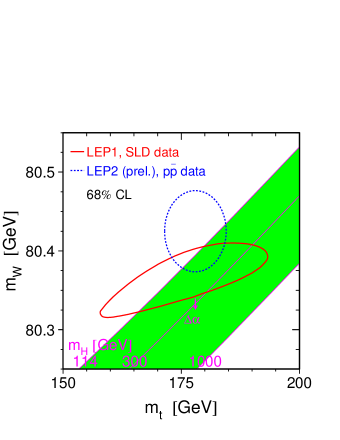
Figure 2: Comparison of the indirect measurements of $M_{W}$ and $m_{t}$ (LEP I+SLD data) (solid contour) and the direct measurement ($p\bar{p}$ colliders and LEP II data) (dashed contour). In both cases the 68% CL contours are plotted. Also shown is the SM relationship for these masses as a function of the Higgs boson mass, $m_{H}$. The arrow labeled $\Delta\alpha$ shows the variation of this relation if $\alpha(M_{Z}^{2})$ is varied by one standard deviation. The left hand side plot is from Ref. ewreport:2005em and corresponds to the Winter 2005 situation (see Eq. 56), the right hand side plot is from the Ref. lepewwg:2005di and corresponds to the Summer 2005 situation (see Eq. 57). The comparison between Winter and Summer 2005 is shown in the right hand side plot.

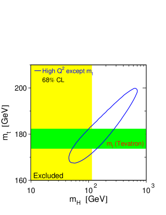
Figure 3: The 68% confidence level contour in $m_{t}$ and $M_{H}$ for the fit to all data except the direct measurement of $m_{t}$, indicated by the shaded horizontal band of $\pm 1\sigma$ width. The vertical band shows the 95% CL exclusion limit on $M_{H}$ from direct searches. From Ref. ewreport:2005em .

The correlation between the Higgs boson mass $M_{H}$, the $W$ boson mass $M_{W}$, the top-quark mass $m_{t}$, and the precision data is illustrated in Figs. 2 and 3. Apart from the impressive agreement existing between the indirect determination of $M_{W}$ and $m_{t}$ and their experimental measurements we see in Fig. 2 that the 68% CL contours from LEP, SLD, and Tevatron measurements select a SM Higgs boson mass region roughly below 200 GeV. Therefore, assuming no physics beyond the Standard Model at the weak scale, all available electroweak precision data are consistent with a light Higgs boson.

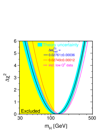
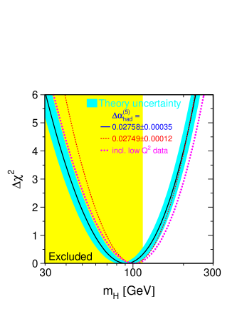
Figure 4: $\Delta\chi^{2}=\chi^{2}-\chi^{2}_{min}$ vs. $M_{H}$ curve. The line is the result of the fit using all electroweak data; the band represents an estimate of the theoretical error due to missing higher order corrections. The vertical band shows the $95\%$ CL exclusion limit on $M_{H}$ from direct searches. The solid and dashed curves are derived using different evaluations of $\Delta\alpha_{had}^{(5)}(M_{Z}^{2})$. The dotted curve includes low $Q^{2}$ data. The left hand side plot is from Ref. ewreport:2005em and corresponds to the Winter 2005 situation (see Eq. 56), the right hand side plot is from the Ref. lepewwg:2005di and corresponds to the Summer 2005 situation (see Eq. 57). Note the different horizontal scale in the two plots.

The actual value of $M_{H}$ emerging from the electroweak precision fits strongly depends on theoretical predictions of physical observables that include different orders of strong and electroweak corrections. As an example, in Fig. 2 the magenta arrow shows how the yellow band would move for one standard deviation variation in the QED fine-structure constant $\alpha(m_{Z}^{2})$. It also depends on the fit input parameters. As we see in Fig. 3, $M_{H}$ grows for larger $m_{t}$. The sensitivity of the indirect bound on $M_{H}$ to $m_{t}$ is clearly visible both in Fig. 2 and in Fig. 4, where you can find the famous blue band plot. In both figures, we compare the results of the Winter 2005 and Summer 2005 electroweak precision fits. As far as the Higgs boson mass goes, the main change between Winter and Summer 2005 has been the value of the top-quark mass. We go from:

$$\left\{\begin{array}[]{l}M_{H}=117^{+67}_{-45}\,\,\,\mbox{GeV}\\ M_{H}<251\,\,\,\mbox{GeV}\,\,\,(95\%\,\,\mbox{CL})\end{array}\right.\,\,\,\,\,\mbox{for}\,\,\,\,\,m_{t}\!=\!178.\pm 4.3\,\,\,\mbox{GeV}\,\,\,.$$ (56)

in Winter 2005 ewreport:2005em , to:

$$\left\{\begin{array}[]{l}M_{H}=91^{+45}_{-32}\,\,\,\mbox{GeV}\\ M_{H}<186-219\,\,\,\mbox{GeV}\,\,\,(95\%\,\,\mbox{CL})\end{array}\right.\,\,\,\,\,\mbox{for}\,\,\,\,\,m_{t}\!=\!172.7\pm 2.9\,\,\,\mbox{GeV}\,\,\,,$$ (57)

in Summer 2005 lepewwg:2005di . We see in Fig. 2 that the overlap between the direct and indirect determination of $M_{H}$ is greatly reduced when the value of $m_{t}$ decreases and at the same time the minimum of the $\Delta\chi^{2}$ band in Fig. 4 considerably shifts. While in the first case the electroweak precision fits are still largely compatible with the direct searches at LEP II that have placed a 95% CL lower bound on $M_{H}$ at:

$$M_{H}>114.4\,\,\,\mbox{GeV}\,\,\,,$$ (58)

in the second case a large region of the $\Delta\chi^{2}$ band in Fig. 4, in particular the region about the minimum, is already excluded, and values of $M_{H}$ very close to the experimental lower bound seem to be favored.

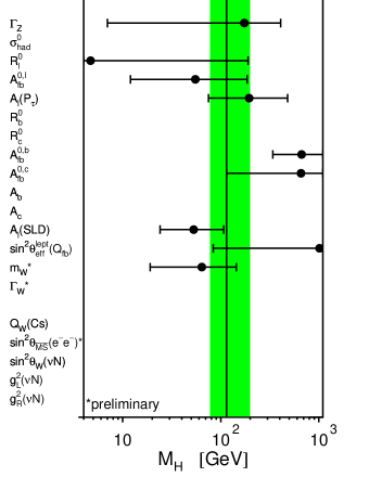
Figure 5: Preferred range for the SM Higgs boson mass $M_{H}$ as determined from various electroweak observables. The shaded band shows the overall constraint on the mass of the Higgs boson as derived from the full data set. From Ref. ewreport:2005em .

It is fair to conclude that the issue of constraining $M_{H}$ from electroweak precision fits is open to controversies and, at a closer look, emerges as a not clear cut statement. With this respect, Fig. 5 illustrates the sensitivity of a few selected electroweak observables to the Higgs boson mass as well as the preferred range for the SM Higgs boson mass as determined from all electroweak observables . One can observe that $M_{W}$ and the leptonic asymmetries prefer a lighter Higgs boson, while $A_{FB}^{b,c}$ and the NuTeV determination of $\sin^{2}\theta_{W}$ prefer a heavier Higgs boson. A certain tension is still present in the data. We could just think that things will progressively adjust and, after the discovery of a light Higgs boson at either the Tevatron or the LHC, this will result in yet another amazing success of the Standard Model. Or, one can interpret the situation depicted in Fig. 5 as an unavoidable indication of the presence of new physics beyond the Standard Model. Indeed, since the data compatible with a lighter Higgs boson are very solid, one could either interpret the data compatible with a larger value of $M_{H}$ as an indication of new physics beyond the Standard Model, or one could drop them as wrong, and still, the Higgs boson mass would turn out to be so small not to be compatible anymore with the Standard Model, signaling once more the presence of new physics.

II.3.4 Fine-tuning

One aspect of the Higgs sector of the Standard Model that is traditionally perceived as problematic is that higher order corrections to the Higgs boson mass parameter square contain quadratic ultraviolet divergences. This is expected in a $\lambda\phi^{4}$ theory and it does not pose a renormalizability problem, since a $\lambda\phi^{4}$ theory is renormalizable. However, although per se renormalizable, these quadratic divergences leave the inelegant feature that the Higgs boson renormalized mass square has to result from the adjusted or fine-tuned balance between a bare Higgs boson mass square and a counterterm that is proportional to the ultraviolet cutoff square. If the physical Higgs mass has to live at the electroweak scale, this can cause a fine-tuning of several orders of magnitude when the scale of new physics $\Lambda$ (the ultraviolet cutoff of the Standard Model interpreted as an effective low energy theory) is well above the electroweak scale. Ultimately this is related to a symmetry principle, or better to the absence of a symmetry principle. Indeed, setting to zero the mass of the scalar fields in the Lagrangian of the Standard Model does not restore any symmetry to the model. Hence, the mass of the scalar fields are not protected against large corrections.

Models of new physics beyond the Standard Model should address this fine-tuning problem and propose a more satisfactory mechanism to obtain the mass of the Higgs particle(s) around the electroweak scale. Supersymmetric models, for instance, have the remarkable feature that fermionic and bosonic degrees of freedom conspire to cancel the Higgs mass quadratic loop divergence, when the symmetry is exact. Other non supersymmetric models, like little Higgs models, address the problem differently, by interpreting the Higgs boson as a Goldstone boson of some global approximate symmetry. In both cases the Higgs mass turns out to be proportional to some small deviation from an exact symmetry principle, and therefore intrinsically small.

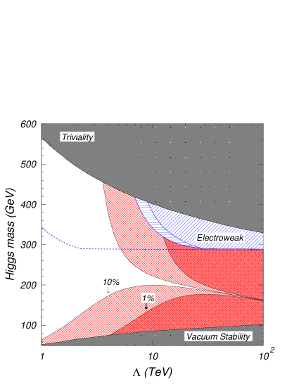
Figure 6: The SM Higgs boson mass $M_{H}$ as a function of the scale of new physics $\Lambda$, with all the constraints derived from unitarity, triviality, vacuum stability, electroweak precision fits, and the requirement of a limited fine-tuning. The empty region is consistent with all the constraints and less than 1 part in 10 fine-tuning. From Ref. Kolda:2000wi .

As suggested in Ref. Kolda:2000wi , the no fine-tuning condition in the Standard Model can be softened and translated into a maximum amount of allowed fine-tuning, that can be directly related to the scale of new physics. As derived in Section II.1, upon spontaneous breaking of the electroweak symmetry, the SM Higgs boson mass at tree level is given by $M_{H}^{2}\!=\!-2\mu^{2}$, where $\mu^{2}$ is the coefficient of the quadratic term in the scalar potential. Higher order corrections to $M_{H}^{2}$ can therefore be calculated as loop corrections to $\mu^{2}$, i.e. by studying how the effective potential in Eq. (16) and its minimum condition are modified by loop corrections. If we interpret the Standard Model as the electroweak scale effective limit of a more general theory living at a high scale $\Lambda$, then the most general form of $\mu^{2}$ including all loop corrections is:

$$\bar{\mu}^{2}=\mu^{2}+\Lambda^{2}\sum_{n=0}^{\infty}c_{n}(\lambda_{i})\log^{n}(\Lambda/Q)\,\,\,,$$ (59)

where $Q$ is the renormalization scale, $\lambda_{i}$ are a set of input parameters (couplings) and the $c_{n}$ coefficients can be deduced from the calculation of the effective potential at each loop order. As noted originally by Veltman, there would be no fine-tuning problem if the coefficient of $\Lambda^{2}$ in Eq. (59) were zero, i.e. if the loop corrections to $\mu^{2}$ had to vanish. This condition, known as Veltman condition, is usually over constraining, since the number of independent $c_{n}$ (set to zero by the Veltman condition) can be larger than the number of inputs $\lambda_{i}$. However the Veltman condition can be relaxed, by requiring that only the sum of a finite number of terms in the coefficient of $\Lambda^{2}$ is zero, i.e. requiring that:

$$\sum_{0}^{n_{max}}c_{n}(\lambda_{i})\log^{n}(\Lambda/M_{H})=0\,\,\,,$$ (60)

where the renormalization scale $\mu$ has been arbitrarily set to $M_{H}$ and the order $n$ has been set to $n_{max}$, fixed by the required order of loop in the calculation of $V_{eff}$. This is based on the fact that higher orders in $n$ come from higher loop effects and are therefore suppressed by powers of $(16\pi^{2})^{-1}$. Limiting $n$ to $n_{max}$, Eq. (60) can now have a solution. Indeed, if the scale of new physics $\Lambda$ is not too far from the electroweak scale, then the Veltman condition in Eq. (60) can be softened even more by requiring that:

$$\sum_{0}^{n_{max}}c_{n}(\lambda_{i})\log^{n}(\Lambda/M_{H})<\frac{v^{2}}{\Lambda^{2}}\,\,\,.$$ (61)

This condition determines a value of $\Lambda_{max}$ such that for $\Lambda\leq\Lambda_{max}$ the stability of the electroweak scale does not require any dramatic cancellation in $\bar{\mu}^{2}$. In other words, for $\Lambda\leq\Lambda_{max}$ the renormalization of the SM Higgs boson mass does not require any fine-tuning. As an example, for $n_{max}\!=\!0$, $c_{0}\!=\!(32\pi^{2}v^{2})^{-1}3(2M_{W}^{2}+M_{Z}^{2}+M_{H}^{2}-4m_{t}^{2})$, and the stability of the electroweak scale is assured up to $\Lambda$ of the order of $4\pi v\simeq 2$ TeV. For $n_{max}\!=\!1$ the maximum $\Lambda$ is pushed up to $\Lambda\simeq 15$ TeV and for $n_{max}\!=\!2$ up to $\Lambda\simeq 50$ TeV. So, just going up to 2-loops assures us that we can consider the SM Higgs sector free of fine-tuning up to scales that are well beyond where we would hope to soon discover new physics.

For each value of $n_{max}$, and for each corresponding $\Lambda_{max}$, $M_{H}$ becomes a function of the cutoff $\Lambda$, and the amount of fine-tuning allowed in the theory limits the region in the $(\Lambda,M_{H})$ plane allowed to $M_{H}(\Lambda)$. This is well represented in Fig. 6, where also the constraint from the conditions of unitarity (see Section II.3.1), triviality (see Section II.3.2), vacuum stability (see Section II.3.2) and electroweak precision fits (see Section II.3.3) are summarized. Finally, the main lesson we take away from this plot is that if a Higgs boson is discovered new physics is just around the corner and should manifest itself at the LHC.

II.4 The Higgs sector of the Minimal Supersymmetric Standard Model

In the supersymmetric extension of the Standard Model, the electroweak symmetry is spontaneously broken via the Higgs mechanism introducing two complex scalar $SU(2)_{L}$ doublets. The dynamics of the Higgs mechanism goes pretty much unchanged with respect to the Standard Model case, although the form of the scalar potential is more complex and its minimization more involved. As a result, the $W^{\pm}$ and $Z^{0}$ weak gauge bosons acquire masses that depend on the parameterization of the supersymmetric model at hand. At the same time, fermion masses are generated by coupling the two scalar doublets to the fermions via Yukawa interactions. A supersymmetric model is therefore a natural reference to compare the Standard Model to, since it is a theoretically sound extension of the Standard Model, still fundamentally based on the same electroweak symmetry breaking mechanism.

Far from being a simple generalization of the SM Higgs sector, the scalar sector of a supersymmetric model can be theoretically more satisfactory because: (i) spontaneous symmetry breaking is radiatively induced (i.e. the sign of the quadratic term in the Higgs potential is driven from positive to negative) mainly by the evolution of the top-quark Yukawa coupling from the scale of supersymmetry-breaking to the electroweak scale, and (ii) higher order corrections to the Higgs mass do not contain quadratic divergences, since they cancel when the contribution of both scalars and their super-partners is considered (see Section II.3.4).

At the same time, the fact of having a supersymmetric theory and two scalar doublets modifies the phenomenological properties of the supersymmetric physical scalar fields dramatically. In this Section we will review only the most important properties of the Higgs sector of the MSSM, so that in Section III we can compare the physics of the SM Higgs boson to that of the MSSM Higgs bosons.

I will start by recalling some general properties of a Two Higgs Doublet Model in Section II.4.1, and I will then specify the discussion to the case of the MSSM in Section II.4.2. In Sections II.4.3 and II.4.4 I will review the form of the couplings of the MSSM Higgs bosons to the SM gauge bosons and fermions, including the impact of the most important supersymmetric higher order corrections. A thorough introduction to Supersymmetry and the Minimal Supersymmetric Standard Model has been given during this school by Prof. H. Haber to whose lectures I refer Haber:tasi04 .

II.4.1 About Two Higgs Doublet Models

The most popular and simplest extension of the Standard Model is obtained by considering a scalar sector made of two instead of one complex scalar doublets. These models, dubbed Two Higgs Doublet Models (2HDM), have a richer spectrum of physical scalar fields. Indeed, after spontaneous symmetry breaking, only three of the eight original scalar degrees of freedom (corresponding to two complex doublet) are reabsorbed in transforming the originally massless vector bosons into massive ones. The remaining five degrees of freedom correspond to physical degrees of freedom in the form of: two neutral scalar, one neutral pseudoscalar, and two charged scalar fields.

At the same time, having multiple scalar doublets in the Yukawa Lagrangian (see Eq. (34)) allows for scalar flavor changing neutral current. Indeed, when generalized to the case of two scalar doublet $\phi^{1}$ and $\phi^{2}$, Eq. (34) becomes (quark case only):

$$\mathcal{L}_{Yukawa}=-\sum_{k=1,2}\Gamma_{ij,k}^{u}\bar{Q}^{i}_{L}\Phi^{k,c}u^{j}_{R}-\sum_{k=1,2}\Gamma_{ij,k}^{d}\bar{Q}^{i}_{L}\Phi^{k}d^{j}_{R}+\mathrm{h.c.}\,\,\,,$$ (62)

where each pair of fermions $(i,j)$ couple to a linear combination of the scalar fields $\phi^{1}$ and $\phi^{2}$. When, upon spontaneous symmetry breaking, the fields $\phi^{1}$ and $\phi^{2}$ acquire vacuum expectation values

$$\langle\Phi^{k}\rangle=\frac{v^{k}}{\sqrt{2}}\,\,\,\,\,\mbox{for}\,\,\,\,\,k=1,2\,\,\,,$$ (63)

the reparameterization of $\mathcal{L}_{Yukawa}$ of Eq. (62) in the vicinity of the minimum of the scalar potential, with $\Phi^{k}=\Phi^{\prime k}+v^{k}$ (for $k=1,2$), gives:

$$\mathcal{L}_{Yukawa}=-\bar{u}^{i}_{L}\underbrace{\sum_{k}\Gamma_{ij,k}^{u}\frac{v^{k}}{\sqrt{2}}}_{M^{u}_{ij}}u^{j}_{R}-\bar{d}^{i}_{L}\underbrace{\sum_{k}\Gamma_{ij,k}^{d}\frac{v^{k}}{\sqrt{2}}}_{M^{d}_{ij}}d^{j}_{R}+\mathrm{h.c.}+\mbox{\small{FC couplings}}\,\,\,,$$ (64)

where the fermion mass matrices $M^{u}_{ij}$ and $M^{d}_{ij}$ are now proportional to a linear combination of the vacuum expectation values of $\phi^{1}$ and $\phi^{2}$. The diagonalization of $M^{u}_{ij}$ and $M^{d}_{ij}$ does not imply the diagonalization of the couplings of the $\phi^{\prime k}$ fields to the fermions, and Flavor Changing (FC) couplings arise. This is perceived as a problem in view of the absence of experimental evidence to support neutral flavor changing effects. If present, these effects have to be tiny in most processes involving in particular the first two generations of quarks, and a safer way to build a 2HDM is to forbid them all together at the Lagrangian level. This is traditionally done by requiring either that $u$-type and $d$-type quarks couple to the same doublet (Model I) or that $u$-type quarks couple to one scalar doublet while $d$-type quarks to the other (Model II). Indeed, these two different realization of a 2HDM can be justified by enforcing on $\mathcal{L}_{Yukawa}$ the following ad hoc discrete symmetry:

$$\left\{\begin{array}[]{c}\Phi^{1}\rightarrow-\Phi^{1}\,\,\,\,\mathrm{and}\,\,\,\,\Phi^{2}\rightarrow\Phi^{2}\\ d^{i}\rightarrow-d^{i}\,\,\,\,\mathrm{and}\,\,\,\,u^{j}\rightarrow\pm u^{j}\end{array}\right.$$ (65)

The case in which FC scalar neutral current are not forbidden (Model III) has also been studied in detail. In this case both up and down-type quarks can couple to both scalar doublets, and strict constraints have to be imposed on the FC scalar couplings in particular between the first two generations of quarks.

2HDMs have indeed a very rich phenomenology that has been extensively studied. In these lectures, however, we will only compare the SM Higgs boson phenomenology to the phenomenology of the Higgs bosons of the MSSM, a particular kind of 2HDM that we will illustrate in the following Sections.

II.4.2 The MSSM Higgs sector: introduction

The Higgs sector of the MSSM is actually a Model II 2HDM. It contains two complex $SU(2)_{L}$ scalar doublets:

$$\Phi_{1}=\left(\begin{array}[]{c}\phi_{1}^{+}\\ \phi_{1}^{0}\end{array}\right)\,\,\,\,\,\,,\,\,\,\,\,\,\Phi_{2}=\left(\begin{array}[]{c}\phi_{2}^{0}\\ \phi_{2}^{-}\end{array}\right)\,\,\,,$$ (66)

with opposite hypercharge ($Y\!=\!\pm 1$), as needed to make the theory anomaly-free. $\Phi_{1}$ couples to the up-type and $\Phi_{2}$ to the down-type quarks respectively. Correspondingly, the Higgs part of the superpotential can be written as:

$$V_{H} = (|\mu|^{2}+m_{1}^{2})|\Phi_{1}|^{2}+(|\mu|^{2}+m_{2}^{2})|\Phi_{2}|^{2}-\mu B\epsilon_{ij}(\Phi_{1}^{i}\Phi_{2}^{j}+h.c.)$$ (67)

$$+ \frac{g^{2}+g^{\prime 2}}{8}\left(|\Phi_{1}|^{2}-|\Phi_{2}|^{2}\right)^{2}+\frac{g^{2}}{2}|\Phi_{1}^{\dagger}\Phi_{2}|^{2}\,\,\,,$$

in which we can identify three different contributions Haber:tasi04 ; Djouadi:2005gj :

• the so called $D$ terms, containing the quartic scalar interactions, which for the Higgs fields $\Phi_{1}$ and $\Phi_{2}$ correspond to:

  $$\frac{g^{2}+g^{\prime 2}}{8}\left(|\Phi_{1}|^{2}-|\Phi_{2}|^{2}\right)^{2}+\frac{g^{2}}{2}|\Phi_{1}^{\dagger}\Phi_{2}|^{2}\,\,\,,$$ (68)

  with $g$ and $g^{\prime}$ the gauge couplings of $SU(2)_{L}$ and $U(1)_{Y}$ respectively;

• the so called $F$ terms, corresponding to:

  $$|\mu|^{2}(|\Phi_{1}|^{2}+|\Phi_{2}|^{2})\,\,\,;$$ (69)

• the soft SUSY-breaking scalar Higgs mass and bilinear terms, corresponding to:

  $$m_{1}^{2}|\Phi_{1}|^{2}+m_{2}^{2}|\Phi_{2}|^{2}-\mu B\epsilon_{ij}(\Phi_{1}^{i}\Phi_{2}^{j}+h.c.)\,\,\,.$$ (70)

Overall, the scalar potential in Eq. (67) depends on three independent combinations of parameters, $|\mu|^{2}+m_{1}^{2}$, $|\mu|^{2}+m_{2}^{2}$, and $\mu B$. One basic difference with respect to the SM case is that the quartic coupling has been replaced by gauge couplings. This reduced arbitrariness will play an important role in the following.

Upon spontaneous symmetry breaking, the neutral components of $\Phi_{1}$ and $\Phi_{2}$ acquire vacuum expectation values

$$\langle\Phi_{1}\rangle=\frac{1}{\sqrt{2}}\left(\begin{array}[]{c}0\\ v_{1}\end{array}\right)\,\,\,\,\,\,,\,\,\,\,\,\,\langle\Phi_{2}\rangle=\frac{1}{\sqrt{2}}\left(\begin{array}[]{c}v_{2}\\ 0\end{array}\right)\,\,\,,$$ (71)

and the Higgs mechanism proceed as in the Standard Model except that now one starts with eight degrees of freedom, corresponding to the two complex doublets $\Phi_{1}$ and $\Phi_{2}$. Three degrees of freedom are absorbed in making the $W^{\pm}$ and the $Z^{0}$ massive. The $W$ mass is chosen to be: $M_{W}^{2}=g^{2}(v_{1}^{2}+v_{2}^{2})/4=g^{2}v^{2}/4$, and this fixes the normalization of $v_{1}$ and $v_{2}$, leaving only two independent parameters to describe the entire MSSM Higgs sector. The remaining five degrees of freedom are physical and correspond to two neutral scalar fields

$$h^{0} = -(\sqrt{2}\mbox{Re}\phi_{2}^{0}-v_{2})\sin\alpha+(\sqrt{2}\mbox{Re}\phi_{1}^{0}-v_{1})\cos\alpha$$ (72)

$$H^{0} = (\sqrt{2}\mbox{Re}\phi_{2}^{0}-v_{2})\cos\alpha+(\sqrt{2}\mbox{Re}\phi_{1}^{0}-v_{1})\sin\alpha\,\,\,,$$

one neutral pseudoscalar field

$$A^{0}=\sqrt{2}\left(\mbox{Im}\phi_{2}^{0}\sin\beta+\mbox{Im}\phi_{1}^{0}\cos\beta\right)\,\,\,,$$ (73)

and two charged scalar fields

$$H^{\pm}=\phi_{2}^{\pm}\sin\beta+\phi_{1}^{\pm}\cos\beta\,\,\,,$$ (74)

where $\alpha$ and $\beta$ are mixing angles, and $\tan\beta\!=\!v_{1}/v_{2}$. At tree level, the masses of the scalar and pseudoscalar degrees of freedom satisfy the following relations:

$$M_{H^{\pm}}^{2} = M_{A}^{2}+M_{W}^{2}\,\,\,,$$ (75)

$$M_{H,h}^{2} = \frac{1}{2}\left(M_{A}^{2}+M_{Z}^{2}\pm((M_{A}^{2}+M_{Z}^{2})^{2}-4M_{Z}^{2}M_{A}^{2}\cos^{2}2\beta)^{1/2}\right)\,\,\,,$$

making it natural to pick $M_{A}$ and $\tan\beta$ as the two independent parameters of the Higgs sector.

Eq. (75) provides the famous tree level upper bound on the mass of one of the neutral scalar Higgs bosons, $h^{0}$:

$$M_{h}^{2}\leq M_{Z}^{2}\cos 2\beta\leq M_{Z}^{2}\,\,\,,$$ (76)

which already contradicts the current experimental lower bound set by LEP II: $M_{h}>93.0$ GeV lephwg:2004mssm . The contradiction is lifted by including higher order radiative corrections to the Higgs spectrum, in particular by calculating higher order corrections to the neutral scalar mass matrix. Over the past few years a huge effort has been dedicated to the calculation of the full one-loop corrections and of several leading and sub-leading sets of two-loop corrections, including resummation of leading and sub-leading logarithms via appropriate renormalization group equation (RGE) methods. A detailed discussion of this topic can be found in some recent reviews Carena:2002es ; Heinemeyer:2004ms ; Heinemeyer:2004gx and in the original literature referenced therein. For the purpose of these lectures, let us just observe that, qualitatively, the impact of radiative corrections on $M_{h}^{max}$ can be seen by just including the leading two-loop corrections proportional to $y_{t}^{2}$, the square of the top-quark Yukawa coupling, and applying RGE techniques to resum the leading orders of logarithms. In this case, the upper bound on the light neutral scalar in Eq. (76) is modified as follows:

$$M_{h}^{2}\leq M_{Z}^{2}+\frac{3g^{2}m_{t}^{2}}{8\pi^{2}M_{W}^{2}}\left[\log\left(\frac{M_{S}^{2}}{m_{t}^{2}}\right)+\frac{X_{t}^{2}}{M_{S}^{2}}\left(1-\frac{X_{t}^{2}}{12M_{S}^{2}}\right)\right]\,\,\,,$$ (77)

where $M_{S}^{2}=(M_{\tilde{t}_{1}}^{2}+M_{\tilde{t}_{2}}^{2})/2$ is the average of the two top-squark masses, $m_{t}$ is the running top-quark mass (to account for the leading two-loop QCD corrections), and $X_{t}$ is the top-squark mixing parameter defined by the top-squark mass matrix:

$$\left(\begin{array}[]{cc}M_{Q_{t}}^{2}+m_{t}^{2}+D_{L}^{t}&m_{t}X_{t}\\ m_{t}X_{t}&M_{R_{t}}^{2}+m_{t}^{2}+D_{R}^{t}\end{array}\right)\,\,\,,$$ (78)

with $X_{t}\equiv A_{t}-\mu\cot\beta$ ($A_{t}$ being one of the top-squark soft SUSY breaking trilinear coupling), $D_{L}^{t}=(1/2-2/3\sin\theta_{W})M_{Z}^{2}\cos 2\beta$, and $D_{R}^{t}=2/3\sin^{2}\theta_{W}M_{Z}^{2}\cos 2\beta$. Fig. 7 illustrates the behavior of $M_{h}$ as a function of $\tan\beta$, in the case of minimal and maximal mixing. For large $\tan\beta$ a plateau (i.e. an upper bound) is clearly reached. The green bands represent the variation of $M_{h}$ as a function of $m_{t}$ when $m_{t}\!=\!175\pm 5$ GeV.

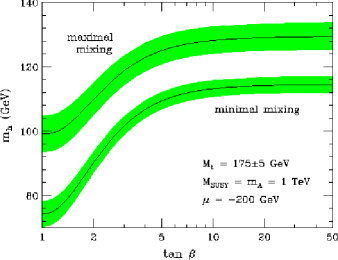
Figure 7: The mass of the light neutral scalar Higgs boson, $h^{0}$, as a function of $\tan\beta$, in the minimal mixing and maximal mixing scenario. The green bands are obtained by varying the top-quark mass in the $m_{t}\!=\!175\pm 5$ GeV range. The plot is built by fixing $M_{A}\!=\!1$ TeV and $M_{SUSY}\!\equiv\!M_{Q}\!=\!\!M_{U}\!=\!M_{D}\!=\!1$ TeV. From Ref. Carena:2002es .

If top-squark mixing is maximal, the upper bound on $M_{h}$ is approximately $M_{h}^{max}\!\simeq\!135$ GeV. The behavior of both $M_{h,H}$ and $M_{H^{\pm}}$ as a function of $M_{A}$ and $\tan\beta$ is summarized in Fig. 8, always for the case of maximal mixing. It is interesting to notice that for all values of $M_{A}$ and $\tan\beta$ the $M_{H}\!>\!M_{h}^{max}$. Also we observe that, in the limit of large $\tan\beta$, i) for $M_{A}\!<\!M_{h}^{max}$: $M_{h}\simeq M_{A}$ and $M_{H}\simeq M_{h}^{max}$, while ii) for $M_{A}\!>\!M_{h}^{max}$: $M_{H}\simeq M_{A}$ and $M_{h}\simeq M_{h}^{max}$.

Figure 8: The mass of the light ($h^{0}$) and heavy ($H^{0}$) neutral scalar Higgs bosons, and of the charged scalar Higgs boson ($H^{\pm}$) as a function of the neutral pseudoscalar mass $M_{A}$, for two different values of $\tan\beta$ ($\tan\beta\!=\!3,30$). The top-quark mass is fixed to $m_{t}\!=\!174.3$ GeV and $M_{SUSY}\!\equiv\!M_{Q}\!=\!\!M_{U}\!=\!M_{D}\!=\!1$ TeV. The maximal mixing scenario is chosen. From Ref. Carena:2002es .

II.4.3 MSSM Higgs boson couplings to electroweak gauge bosons

The Higgs boson couplings to the electroweak gauge bosons are obtained from the kinetic term of the scalar Lagrangian, in strict analogy to what we have explicitly seen in the case of the SM Higgs boson. Here, we would like to recall the form of the $H_{i}VV$ and $H_{i}H_{j}V$ couplings (for $H_{i}\!=\!h^{0},H^{0},A^{0},H^{\pm}$, and $V\!=\!W^{\pm},Z^{0}$) that are most important in order to understand the main features of the MSSM plots that will be shown in Section III.

First of all, the couplings of the neutral scalar Higgs bosons to both $W^{\pm}$ and $Z^{0}$ can be written as:

$$g_{hVV}=g_{V}M_{V}\sin(\beta-\alpha)g^{\mu\nu}\,\,\,\,\,,\,\,\,\,\,g_{HVV}=g_{V}M_{V}\cos(\beta-\alpha)g^{\mu\nu}\,\,\,,$$ (79)

where $g_{V}\!=\!2M_{V}/v$, while the $A^{0}VV$ and $H^{\pm}VV$ couplings vanish because of CP-invariance. As in the SM case, since the photon is massless, there are no tree level $\gamma\gamma H_{i}$ and $\gamma Z^{0}H_{i}$ couplings.

Moreover, in the neutral Higgs sector, only the $h^{0}A^{0}Z^{0}$ and $H^{0}A^{0}Z^{0}$ couplings are allowed and given by:

$$g_{hAZ}=\frac{g\cos(\beta-\alpha)}{2\cos\theta_{W}}(p_{h}-p_{A})^{\mu}\,\,\,\,\,,\,\,\,\,\,g_{HAZ}=-\frac{g\sin(\beta-\alpha)}{2\cos\theta_{W}}(p_{H}-p_{A})^{\mu}\,\,\,,$$ (80)

where all momenta are incoming. We also have several $H_{i}H_{j}V$ couplings involving the charge Higgs boson, namely:

$$g_{H^{+}H^{-}Z} = -\frac{g}{2\cos\theta_{W}}\cos 2\theta_{W}(p_{H^{+}}-p_{H^{-}})^{\mu}\,\,\,,$$ (81)

$$g_{H^{+}H^{-}\gamma} = -ie(p_{H^{+}}-p_{H^{-}})^{\mu}\,\,\,,$$

$$g_{H^{\mp}hW^{\pm}} = \mp i\frac{g}{2}\cos(\beta-\alpha)(p_{h}-p_{H^{\mp}})^{\mu}\,\,\,,$$

$$g_{H^{\mp}HW^{\pm}} = \pm i\frac{g}{2}\sin(\beta-\alpha)(p_{H}-p_{H^{\mp}})^{\mu}\,\,\,,$$

$$g_{H^{\mp}AW^{\pm}} = \frac{g}{2}(p_{A}-p_{H^{\pm}})^{\mu}\,\,\,.$$

At this stage it is interesting to introduce the so called decoupling limit, i.e. the limit of $M_{A}\gg M_{Z}$, and to analyze how masses and couplings behave in this particular limit. $M_{H^{\pm}}$ in Eq. (75) is unchanged, while $M_{h,H}$ become:

$$M_{h}\simeq M_{h}^{max}\,\,\,\,\,\mbox{and}\,\,\,\,\,M_{H}\simeq M_{A}^{2}+M_{Z}^{2}\sin^{2}2\beta\,\,\,.$$ (82)

Moreover, as one can derive from the diagonalization of the neutral scalar Higgs boson mass matrix:

$$\cos^{2}(\beta-\alpha)=\frac{M_{h}^{2}(M_{Z}^{2}-M_{h}^{2})}{M_{A}^{2}(M_{H}^{2}-M_{h}^{2})}\,\,\,\stackrel{{\scriptstyle M_{A}^{2}\gg M_{Z}^{2}}}{{\longrightarrow}}\,\,\,\frac{M_{Z}^{4}\sin^{2}4\beta}{4M_{A}^{4}}\,\,\,.$$ (83)

From the previous equations we then deduce that, in the decoupling limit, the only light Higgs boson is $h^{0}$ with mass $M_{h}\simeq M_{h}^{max}$, while $M_{H}\simeq M_{H^{\pm}}\simeq M_{A}\gg M_{Z}$, and because $\cos(\beta-\alpha)\rightarrow 0$ ($\sin(\beta-\alpha)\rightarrow 1)$), the couplings of $h^{0}$ to the gauge bosons tend to the SM Higgs boson limit. This is to say that, in the decoupling limit, the light MSSM Higgs boson will be hardly distinguishable from the SM Higgs boson.

Finally, we need to remember that the tree level couplings may be modified by radiative corrections involving both loops of SM and MSSM particles, among which loops of third generation quarks and squarks dominate. The very same radiative corrections that modify the Higgs boson mass matrix, thereby changing the definition of the mass eigenstates, also affect the couplings of the corrected mass eigenstates to the gauge bosons. This can be reabsorbed into the definition of a renormalized mixing angle $\alpha$ or a radiatively corrected value for $\cos(\beta-\alpha)$ ($\sin(\beta-\alpha)$). Using the notation of Ref. Carena:2002es , the radiatively corrected $\cos(\beta-\alpha)$ can be written as:

$$\cos(\beta-\alpha)=K\left[\frac{M_{Z}^{2}\sin 4\beta}{2M_{A}^{2}}+\mathcal{O}\left(\frac{M_{Z}^{4}}{M_{A}^{4}}\right)\right]\,\,\,,$$ (84)

where

$$K\equiv 1+\frac{\delta\mathcal{M}_{11}^{2}-\delta\mathcal{M}_{22}^{2}}{2M_{Z}^{2}\cos 2\beta}-\frac{\delta\mathcal{M}_{12}^{2}}{M_{Z}^{2}\sin 2\beta}\,\,\,,$$ (85)

and $\delta\mathcal{M}_{ij}$ are the radiative corrections to the corresponding elements of the CP-even Higgs squared-mass matrix (see Ref. Carena:2002es ). It is interesting to notice that on top of the traditional decoupling limit introduced above ($M_{A}\gg M_{Z}$), there is now also the possibility that $\cos(\beta-\alpha)\rightarrow 0$ if $K\rightarrow 0$, and this happens independently of the value of $M_{A}$.

II.4.4 MSSM Higgs boson couplings to fermions

As anticipated, $\Phi_{1}$ and $\Phi_{2}$ have Yukawa-type couplings to the up-type and down-type components of all $SU(2)_{L}$ fermion doublets. For example, the Yukawa Lagrangian corresponding to the third generation of quarks reads:

$$\mathcal{L}_{Yukawa}=-h_{t}\left[\bar{t}_{R}\phi_{1}^{0}t_{L}-\bar{t}_{R}\phi_{1}^{+}b_{L}\right]-h_{b}\left[\bar{b}_{R}\phi_{2}^{0}b_{L}-\bar{b}_{R}\phi_{2}^{-}t_{L}\right]+\mathrm{h.c.}$$ (86)

Upon spontaneous symmetry breaking $\mathcal{L}_{Yukawa}$ provides both the corresponding quark masses:

$$m_{t}=h_{t}\frac{v_{1}}{\sqrt{2}}=h_{t}\frac{v\sin\beta}{\sqrt{2}}\,\,\,\,\,\mbox{and}\,\,\,\,\,m_{b}=h_{b}\frac{v_{2}}{\sqrt{2}}=h_{b}\frac{v\cos\beta}{\sqrt{2}}\,\,\,,$$ (87)

and the corresponding Higgs-quark couplings:

$$g_{ht\bar{t}} = \frac{\cos\alpha}{\sin\beta}y_{t}=\left[\sin(\beta-\alpha)+\cot\beta\cos(\beta-\alpha)\right]y_{t}\,\,\,,$$ (88)

$$g_{hb\bar{b}} = -\frac{\sin\alpha}{\cos\beta}y_{b}=\left[\sin(\beta-\alpha)-\tan\beta\cos(\beta-\alpha)\right]y_{b}\,\,\,,$$

$$g_{Ht\bar{t}} = \frac{\sin\alpha}{\sin\beta}y_{t}=\left[\cos(\beta-\alpha)-\cot\beta\sin(\beta-\alpha)\right]y_{t}\,\,\,,$$

$$g_{Hb\bar{b}} = \frac{\cos\alpha}{\cos\beta}y_{b}=\left[\cos(\beta-\alpha)+\tan\beta\sin(\beta-\alpha)\right]y_{b}\,\,\,,$$

$$g_{At\bar{t}} = \cot\beta\,y_{t}\,\,\,\,,\,\,\,\,g_{Ab\bar{b}}=\tan\beta\,y_{b}\,\,\,,$$

$$g_{H^{\pm}t\bar{b}} = \frac{g}{2\sqrt{2}M_{W}}\left[m_{t}\cot\beta(1-\gamma_{5})+m_{b}\tan\beta(1+\gamma_{5})\right]\,\,\,,$$

where $y_{q}\!=\!m_{q}/v$ (for $q\!=\!t,b$) are the SM couplings. It is interesting to notice that in the $M_{A}\gg M_{Z}$ decoupling limit, as expected, all the couplings in Eq. (88) reduce to the SM limit, i.e. all $H^{0}$, $A^{0}$, and $H^{\pm}$ couplings vanish, while the couplings of the light neutral Higgs boson, $h^{0}$, reduce to the corresponding SM Higgs boson couplings.

The Higgs boson-fermion couplings are also modified directly by one-loop radiative corrections (squarks-gluino loops for quarks couplings and slepton-neutralino loops for lepton couplings). A detailed discussion can be found in Ref. Carena:2002es ; Djouadi:2005gj and in the literature referenced therein. Of particular relevance are the corrections to the couplings of the third quark generation. These can be parameterized at the Lagrangian level by writing the radiatively corrected effective Yukawa Lagrangian as:

$$\mathcal{L}_{Yukawa}^{eff} = -\epsilon_{ij}\left[(h_{b}+\delta h_{b})\bar{b}_{R}Q^{j}_{L}\Phi^{i}_{2}+(h_{t}+\delta h_{t})\bar{t}_{R}Q^{i}_{L}\Phi^{j}_{1}\right]$$

$$- \Delta h_{t}\bar{t}_{R}Q^{k}_{L}\Phi^{k\ast}_{2}-\Delta h_{b}\bar{b}_{R}Q^{k}_{L}\Phi^{k\ast}_{1}+\mathrm{h.c.}\,\,\,,$$

where we notice that radiative corrections induce a small coupling between $\Phi_{1}$ and down-type fields and between $\Phi_{2}$ and up-type fields. Moreover the tree level relation between $h_{b}$, $h_{t}$, $m_{b}$ and $m_{t}$ are modified as follows:

$$m_{b} = \frac{h_{b}v}{\sqrt{2}}\cos\beta\left(1+\frac{\delta h_{b}}{h_{b}}+\frac{\Delta h_{b}\tan\beta}{h_{b}}\right)\equiv\frac{h_{b}v}{\sqrt{2}}\cos\beta(1+\Delta_{b})\,\,\,,$$ (90)

$$m_{t} = \frac{h_{t}v}{\sqrt{2}}\sin\beta\left(1+\frac{\delta h_{t}}{h_{t}}+\frac{\Delta h_{t}\tan\beta}{h_{t}}\right)\equiv\frac{h_{t}v}{\sqrt{2}}\sin\beta(1+\Delta_{t})\,\,\,,$$

where the leading corrections are proportional to $\Delta h_{b}$ and turn out to also be $\tan\beta$ enhanced. On the other hand, the couplings between Higgs mass eigenstates and third generation quarks given in Eq. (88) are corrected as follows:

$$g_{ht\bar{t}} = \frac{\cos\alpha}{\sin\beta}y_{t}\,\left[1-\frac{1}{1+\Delta_{t}}\frac{\Delta h_{t}}{h_{t}}\left(\cot\beta+\tan\alpha\right)\right]\,\,\,,$$ (91)

$$g_{hb\bar{b}} = -\frac{\sin\alpha}{\cos\beta}y_{b}\,\left[1+\frac{1}{1+\Delta_{b}}\left(\frac{\delta h_{b}}{h_{b}}-\Delta_{b}\right)\left(1+\cot\alpha\cot\beta\right)\right]\,\,\,,$$

$$g_{Ht\bar{t}} = \frac{\sin\alpha}{\sin\beta}y_{t}\,\left[1-\frac{1}{1+\Delta_{t}}\frac{\Delta h_{t}}{h_{t}}\left(\cot\beta-\cot\alpha\right)\right]\,\,\,,$$

$$g_{Hb\bar{b}} = \frac{\cos\alpha}{\cos\beta}y_{b}\,\left[1+\frac{1}{1+\Delta_{b}}\left(\frac{\delta h_{b}}{h_{b}}-\Delta_{b}\right)\left(1-\tan\alpha\cot\beta\right)\right]\,\,\,,$$

$$g_{At\bar{t}} = \cot\beta\,y_{t}\,\left[1-\frac{1}{1+\Delta_{t}}\frac{\Delta h_{t}}{h_{t}}\left(\cot\beta+\tan\beta\right)\right]\,\,\,,$$

$$g_{Ab\bar{b}} = \tan\beta\,y_{b}\,\left[1+\frac{1}{(1+\Delta_{b})\sin^{2}\beta}\left(\frac{\delta h_{b}}{h_{b}}-\Delta_{b}\right)\right]\,\,\,,$$

$$g_{H^{\pm}t\bar{b}} \simeq \frac{g}{2\sqrt{2}M_{W}}\left\{m_{t}\cot\beta\left[1-\frac{1}{1+\Delta_{t}}\frac{\Delta h_{t}}{h_{t}}\left(\cot\beta+\tan\beta\right)\right](1+\gamma_{5})\right.$$

$$+ \left.m_{b}\tan\beta\left[1+\frac{1}{(1+\Delta_{b})\sin^{2}\beta}\left(\frac{\delta h_{b}}{h_{b}}-\Delta_{b}\right)\right](1-\gamma_{5})\right\}\,\,\,,$$

where the last coupling is given in the approximation of small isospin breaking effects, since interactions of this kind have been neglected in the Lagrangian of Eq. (II.4.4).

III Phenomenology of the Higgs Boson

III.1 Standard Model Higgs boson decay branching ratios

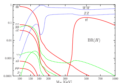
Figure 9: SM Higgs decay branching ratios as a function of $M_{H}$. The blue curves represent tree-level decays into electroweak gauge bosons, the red curves tree level decays into quarks and leptons, the green curves one-loop decays. From Ref. Djouadi:2005gi .

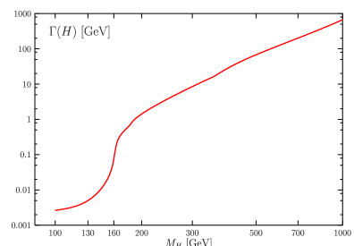
Figure 10: SM Higgs total decay width as a function of $M_{H}$. From Ref. Djouadi:2005gi .

In this Section we approach the physics of the SM Higgs boson by considering its branching ratios for various decay modes. In Section II.2 we have derived the SM Higgs couplings to gauge bosons and fermions. Therefore we know that, at the tree level, the SM Higgs boson can decay into pairs of electroweak gauge bosons ($H\rightarrow W^{+}W^{-},ZZ$), and into pairs of quarks and leptons ($H\rightarrow Q\bar{Q},l^{+}l^{-}$); while at one-loop it can also decay into two photons ($H\rightarrow\gamma\gamma$), two gluons ($H\rightarrow gg$), or a $\gamma Z$ pair ($H\rightarrow\gamma Z$). Fig. 9 represents all the decay branching ratios of the SM Higgs boson as functions of its mass $M_{H}$. The SM Higgs boson total width, sum of all the partial widths $\Gamma(H\rightarrow XX)$, is represented in Fig. 10.

Fig. 9 shows that a light Higgs boson ($M_{H}\leq 130-140$ GeV) behaves very differently from a heavy Higgs boson ($M_{H}\geq 130-140$ GeV). Indeed, a light SM Higgs boson mainly decays into a $b\bar{b}$ pair, followed hierarchically by all other pairs of lighter fermions. Loop-induced decays also play a role in this region. $H\rightarrow gg$ is dominant among them, and it is actually larger than many tree level decays. Unfortunately, this decay mode is almost useless, in particular at hadron colliders, because of background limitations. Among radiative decays, $H\rightarrow\gamma\gamma$ is tiny, but it is actually phenomenologically very important because the two photon signal can be seen over large hadronic backgrounds. On the other hand, for larger Higgs masses, the decays to $W^{+}W^{-}$ and $ZZ$ dominates. All decays into fermions or loop-induced decays are suppressed, except $H\rightarrow t\bar{t}$ for Higgs masses above the $t\bar{t}$ production threshold. There is an intermediate region, around $M_{H}\simeq 160$ GeV, i.e. below the $W^{+}W^{-}$ and $ZZ$ threshold, where the decays into $WW^{*}$ and $ZZ^{*}$ (when one of the two gauge bosons is off-shell) become important. These are indeed three-body decays of the Higgs boson that start to dominate over the $H\rightarrow b\bar{b}$ two-body decay mode when the largeness of the $HWW$ or $HZZ$ couplings compensate for their phase space suppression. The different decay pattern of a light vs a heavy Higgs boson influences the role played, in each mass region, by different Higgs production processes at hadron and lepton colliders.

The curves in Fig. 9 are obtained by including all available QCD and electroweak (EW) radiative corrections. Indeed, the problem of computing the relevant orders of QCD and EW corrections for Higgs decays has been thoroughly explored and the results are nowadays available in public codes like HDECAY Djouadi:1997yw , which has been used to produce Fig. 9. Indeed it would be more accurate to represent each curve as a band, obtained by varying the parameters that enters both at tree level and in particular through loop corrections within their uncertainties. This is shown, for a light and intermediate mass Higgs boson, in Fig. 11 where each band has been obtained including the uncertainty from the quark masses and from the strong coupling constant.

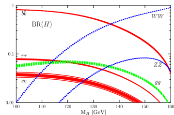
Figure 11: SM Higgs boson decay branching ratios in the low and intermediate Higgs boson mass range including the uncertainty from the quark masses $m_{t}\!=\!178\pm 4.3$ GeV, $m_{b}\!=\!4.88\pm 0.07$ GeV, and $m_{c}\!=\!1.64\pm 0.07$ GeV, as well as from $\alpha_{s}(M_{Z})\!=\!0.1172\pm 0.002$. From Ref. Djouadi:2005gi .

In the following we will briefly review the various SM Higgs decay channels. Giving a schematic but complete list of all available radiative corrections goes beyond the purpose of these lectures. Therefore we will only discuss those aspects that can be useful as a general background. In particular I will comment on the general structure of radiative corrections to Higgs decay and I will add more details on QCD corrections to $H\rightarrow Q\bar{Q}$ ($Q=$ heavy quark).

For a detailed review of QCD correction in Higgs decays we refer the reader to Ref. Spira:1997dg . Ref. Djouadi:2005gi also contain an excellent summary of both QCD and EW radiative corrections to Higgs decays.

III.1.1 General properties of radiative corrections to Higgs decays

All Higgs boson decay rates are modified by both EW and QCD radiative corrections. QCD corrections are particularly important for $H\rightarrow Q\bar{Q}$ decays, where they mainly amount to a redefinition of the Yukawa coupling by shifting the mass parameter in it from the pole mass value to the running mass value, and for $H\rightarrow gg$. EW corrections can be further separated into: i) corrections due to fermion loops, ii) corrections due to the Higgs boson self-interaction, and iii) other EW corrections. Both corrections of type (ii) and (iii) are in general very small if not for large Higgs boson masses, i.e. for $M_{H}\gg M_{W}$. On the other hand, corrections of type (i) are very important over the entire Higgs mass range, and are particularly relevant for $M_{H}\ll 2m_{t}$, where the top-quark loop corrections play a leading role. Indeed, for $M_{H}\ll 2m_{t}$, the dominant corrections for both Higgs decays into fermion and gauge bosons come from the top-quark contribution to the renormalization of the Higgs wave function and vacuum expectation value.

Several higher order radiative corrections to Higgs decays have been calculated in the large $m_{t}$ limit, specifically in the limit when $M_{H}\ll 2m_{t}$. Results can then be derived applying some very powerful low energy theorems. The idea is that, for an on-shell Higgs field ($p_{H}^{2}\!=\!M_{H}^{2}$), the limit of small masses ($M_{H}\ll 2m_{t}$) is equivalent to a $p_{H}\rightarrow 0$ limit, in which case the Higgs couplings to the fermion fields can be simply obtained by substituting

$$m_{i}^{0}\rightarrow m_{i}^{0}\left(1+\frac{H^{0}}{v^{0}}\right)\,\,\,,$$ (92)

in the (bare) Yukawa Lagrangian, for each massive particle $i$. In Eq. (92) $H^{0}$ is a constant field and the upper zero indices indicate that all formal manipulations are done on bare quantities. This induces a simple relation between the bare matrix element for a process with ($X\rightarrow Y+H$) and without ($X\rightarrow Y$) a Higgs field, namely

$$\lim_{p_{H}\rightarrow 0}\mathcal{A}(X\rightarrow Y+H)=\frac{1}{v^{0}}\sum_{i}m_{i}^{0}\frac{\partial}{\partial m_{i}^{0}}\mathcal{A}(X\rightarrow Y)\,\,\,.$$ (93)

When the theory is renormalized, the only actual difference is that the derivative operation in Eq. (93) needs to be modified as follows

$$m_{i}^{0}\frac{\partial}{\partial m_{i}^{0}}\longrightarrow\frac{m_{i}}{1+\gamma_{m_{i}}}\frac{\partial}{\partial m_{i}}$$ (94)

where $\gamma_{m_{i}}$ is the mass anomalous dimension of fermion $f_{i}$. This accounts for the fact that the renormalized Higgs-fermion Yukawa coupling is determined through the $Z_{2}$ and $Z_{m}$ counterterms, and not via the $Hf\bar{f}$ vertex function at zero momentum transfer (as used in the $p_{H}\to 0$ limit above).

The theorem summarized by Eq. (93) is valid also when higher order radiative corrections are included. Therefore, outstanding applications of Eq. (93) include the determination of the one-loop $Hgg$ and $H\gamma\gamma$ vertices from the gluon or photon self-energies, as well as the calculation of several orders of their QCD and EW radiative corrections. Indeed, in the $m_{t}\rightarrow\infty$ limit, the loop-induced $H\gamma\gamma$ and $Hgg$ interactions can be seen as effective vertices derived from an effective Lagrangian of the form:

$$\mathcal{L}_{eff}=\frac{\alpha_{s}}{12\pi}F^{(a)\mu\nu}F^{(}a)_{\mu\nu}\frac{H}{v}(1+O(\alpha_{s}))\,\,\,,$$ (95)

where $F^{(}a)_{\mu\nu}$ is the field strength tensor of QED (for the $H\gamma\gamma$ vertex) or QCD (for the $Hgg$ vertex). The calculation of higher order corrections to the $H\rightarrow\gamma\gamma$ and $H\rightarrow gg$ decays is then reduced by one order of loops! Since these vertices start as one-loop effects, the calculation of the first order of corrections would already be a strenuous task, and any higher order effect would be a formidable challenge. Thanks to the low energy theorem results sketched above, QCD NNLO corrections have indeed been calculated.

III.1.2 Higgs boson decays to gauge bosons: $H\rightarrow W^{+}W^{-},ZZ$

The tree level decay rate for $H\rightarrow VV$ ($V\!=\!W^{\pm},Z$) can be written as:

$$\Gamma(H\rightarrow VV)=\frac{G_{F}M_{H}^{3}}{16\sqrt{2}\pi}\delta_{V}\left(1-\tau_{V}+\frac{3}{4}\tau_{V}^{2}\right)\beta_{V}\,\,\,,$$ (96)

where $\beta_{V}=\sqrt{1-\tau_{V}}$, $\tau_{V}=4M_{V}^{2}/M_{H}^{2}$, and $\delta_{W,Z}\!=\!2,1$.

Below the $W^{+}W^{-}$ and $ZZ$ threshold, the SM Higgs boson can still decay via three (or four) body decays mediated by $WW^{*}$ ($W^{*}W^{*}$) or $ZZ^{*}$ ($Z^{*}Z^{*}$) intermediate states. As we can see from Fig. 9, the off-shell decays $H\rightarrow WW^{*}$ and $H\rightarrow ZZ^{*}$ are relevant in the intermediate mass region around $M_{H}\simeq 160$ GeV, where they compete and overcome the $H\rightarrow b\bar{b}$ decay mode. The decay rates for $H\rightarrow VV^{*}\rightarrow Vf_{i}\bar{f_{j}}$ ($V\!=\!W^{\pm},Z$) are given by:

$$\Gamma(H\rightarrow WW^{*}) = \frac{3g^{4}M_{H}}{512\pi^{3}}F\left(\frac{M_{W}}{M_{H}}\right)\,\,\,,$$ (97)

$$\Gamma(H\rightarrow ZZ^{*}) = \frac{g^{4}M_{H}}{2048(1-s_{W}^{2})^{2}\pi^{3}}\left(7-\frac{40}{3}s_{W}^{2}+\frac{160}{9}s_{W}^{4}\right)F\left(\frac{M_{Z}}{M_{H}}\right)\,\,\,,$$

where $s_{W}\!=\!\sin\theta_{W}$ is the sine of the Weinberg angle and the function $F(x)$ is given by

$$F(x) = -(1-x^{2})\left(\frac{47}{2}x^{2}-\frac{13}{2}+\frac{1}{x^{2}}\right)-3\left(1-6x^{2}+4x^{4}\right)\ln(x)$$ (98)

$$+ 3\,\frac{1-8x^{2}+20x^{4}}{\sqrt{4x^{2}-1}}\arccos\left(\frac{3x^{2}-1}{2x^{3}}\right)\,\,\,.$$

III.1.3 Higgs boson decays to fermions: $H\rightarrow Q\bar{Q},l^{+}l^{-}$

The tree level decay rate for $H\rightarrow f\bar{f}$ ($f\!=\!Q,l$, $Q=$quark, $l=$lepton) can be written as:

$$\Gamma(H\rightarrow f\bar{f})=\frac{G_{F}M_{H}}{4\sqrt{2}\pi}N_{c}^{f}m_{f}^{2}\beta_{f}^{3}\,\,\,,$$ (99)

where $\beta_{f}=\sqrt{1-\tau_{f}}$, $\tau_{f}=4m_{f}^{2}/M_{H}^{2}$, and $(N_{c})^{l,Q}\!=\!1,3$. QCD corrections dominate over other radiative corrections and they modify the rate as follows:

$$\Gamma(H\rightarrow Q\bar{Q})_{QCD}=\frac{3G_{F}M_{H}}{4\sqrt{2}\pi}\bar{m}_{Q}^{2}(M_{H})\beta_{q}^{3}\left[\Delta_{QCD}+\Delta_{t}\right]\,\,\,,$$ (100)

where $\Delta_{t}$ represents specifically QCD corrections involving a top-quark loop. $\Delta_{QCD}$ and $\Delta_{t}$ have been calculated up to three loops and are given by:

$$\Delta_{QCD} = 1+5.67\frac{\alpha_{s}(M_{H})}{\pi}+(35.94-1.36N_{F})\left(\frac{\alpha_{s}(M_{H})}{\pi}\right)^{2}+$$

$$(164.14-25.77N_{F}+0.26N_{F}^{2})\left(\frac{\alpha_{s}(M_{H})}{\pi}\right)^{3}\,\,\,,$$

$$\Delta_{t} = \left(\frac{\alpha_{s}(M_{H})}{\pi}\right)^{2}\left[1.57-\frac{2}{3}\ln\frac{M_{H}^{2}}{m_{t}^{2}}+\frac{1}{9}\ln^{2}\frac{\bar{m}_{Q}^{2}(M_{H})}{M_{H}^{2}}\right]\,\,\,,$$

where $\alpha_{s}(M_{H})$ and $\bar{m}_{Q}(M_{H})$ are the renormalized running QCD coupling and quark mass in the $\overline{MS}$ scheme. It is important to notice that using the $\overline{MS}$ running mass in the overall Yukawa coupling square of Eq. (100)is very important in Higgs decays, since it reabsorbs most of the QCD corrections, including large logarithms of the form $\ln(M_{H}^{2}/m_{Q}^{2})$. Indeed, for a generic scale $\mu$, $\bar{m}_{Q}(\mu)$ is given at leading order by:

$$\bar{m}_{Q}(\mu)_{LO} = \bar{m}_{Q}(m_{Q})\left(\frac{\alpha_{s}(\mu)}{\alpha_{s}(m_{Q})}\right)^{\frac{2b_{0}}{\gamma_{0}}}$$

$$= \bar{m}_{Q}(m_{Q})\left(1-\frac{\alpha_{s}(\mu)}{4\pi}\ln\left(\frac{\mu^{2}}{m_{Q}^{2}}\right)+\cdots\right)\,\,\,,$$

where $b_{0}$ and $\gamma_{0}$ are the first coefficients of the $\beta$ and $\gamma$ functions of QCD, while at higher orders it reads:

$$\bar{m}_{Q}(\mu)=\bar{m}_{Q}(m_{Q})\frac{f\left(\alpha_{s}(\mu)/\pi\right)}{f\left(\alpha_{s}(m_{Q})/\pi\right)}\,\,\,,$$ (103)

where, from renormalization group techniques, the function $f(x)$ is of the form:

$$f(x) = \left(\frac{25}{6}x\right)^{\frac{12}{25}}\left[1+1.014x+\ldots\right]\,\,\,\,\,\,\mbox{for}\,\,\,\,\,m_{c}\!<\!\mu\!<\!m_{b}\,\,\,,$$ (104)

$$f(x) = \left(\frac{23}{6}x\right)^{\frac{12}{23}}\left[1+1.175x+\ldots\right]\,\,\,\,\,\,\mbox{for}\,\,\,\,\,m_{b}\!<\!\mu\!<\!m_{t}\,\,\,,$$

$$f(x) = \left(\frac{7}{2}x\right)^{\frac{4}{7}}\left[1+1.398x+\ldots\right]\,\,\,\,\,\,\mbox{for}\,\,\,\,\,\mu\!>\!m_{t}\,\,\,.$$

As we can see from Eqs. (103) and (104), by using the $\overline{MS}$ running mass, leading and subleading logarithms up to the order of the calculation are actually resummed at all orders in $\alpha_{s}$.

The overall mass factor coming from the quark Yukawa coupling square is actually the only place where we want to employ a running mass. For quarks like the $b$ quark this could indeed have a large impact, since, in going from $\mu\simeq M_{H}$ to $\mu\simeq m_{b}$, $\bar{m}_{n}(\mu)$ varies by almost a factor of two, making therefore almost a factor of four at the rate level. All other mass corrections, in the matrix element and phase space entering the calculation of the $H\rightarrow Q\bar{Q}$ decay rate, can in first approximation be safely neglected.

III.1.4 Loop induced Higgs boson decays: $H\rightarrow\gamma\gamma,\gamma Z,gg$

As seen in Section II.2, the $H\gamma\gamma$ and $H\gamma Z$ couplings are induced at one loop via both a fermion loop and a W-loop. At the lowest order the decay rate for $H\rightarrow\gamma\gamma$ can be written as:

$$\Gamma(H\rightarrow\gamma\gamma)=\frac{G_{F}\alpha^{2}M_{H}^{3}}{128\sqrt{2}\pi^{3}}\left|\sum_{f}N_{c}^{f}Q_{f}^{2}A_{f}^{H}(\tau_{f})+A_{W}^{H}(\tau_{W})\right|^{2}\,\,\,,$$ (105)

where $N_{c}^{f}=1,3$ (for $f=l,q$ respectively), $Q_{f}$ is the charge of the $f$ fermion species, $\tau_{f}=4m_{f}^{2}/M_{H}^{2}$, the function $f(\tau)$ is defined as:

$$f(\tau)=\left\{\begin{array}[]{lr}\arcsin^{2}\frac{1}{\sqrt{\tau}}&\tau\geq 1\\ -\frac{1}{4}\left[\ln\frac{1+\sqrt{1-\tau}}{1-\sqrt{1-\tau}}-i\pi\right]^{2}&\tau<1\,\,\,,\end{array}\right.$$ (106)

and the form factors $A_{f}^{H}$ and $A_{W}^{H}$ are given by:

$$A_{f}^{H} = 2\tau\left[1+(1-\tau)f(\tau)\right]\,\,\,,$$ (107)

$$A_{W}^{H}(\tau) = -\left[2+3\tau+3\tau(2-\tau)f(\tau)\right]\,\,\,.$$

On the other hand, the decay rate for $H\rightarrow\gamma Z$ is given by:

$$\Gamma(H\rightarrow\gamma Z)=\frac{G_{F}^{2}M_{W}^{2}\alpha M_{H}^{3}}{64\pi^{4}}\left(1-\frac{M_{Z}^{2}}{M_{H}^{2}}\right)^{3}\left|\sum_{f}A_{f}^{H}(\tau_{f},\lambda_{f})+A_{W}^{H}(\tau_{W},\lambda_{W})\right|^{2}\,\,\,,$$ (108)

where $\tau_{i}\!=\!4M_{i}^{2}/M_{H}^{2}$ and $\lambda_{i}\!=\!4M_{i}^{2}/M_{Z}^{2}$ ($i\!=\!f,W$), and the form factors $A_{f}^{H}(\tau,\lambda)$ and $A_{W}^{H}(\tau,\lambda)$ are given by:

$$A_{f}^{H}(\tau,\lambda) = 2N_{c}^{f}\frac{Q_{f}(I_{3f}-2Q_{f}\sin^{2}\theta_{W})}{\cos\theta_{W}}\left[I_{1}(\tau,\lambda)-I_{2}(\tau,\lambda)\right]\,\,\,,$$ (109)

$$A_{W}^{H}(\tau,\lambda) = \cos\theta_{W}\left\{\left[\left(1+\frac{2}{\tau}\right)\tan^{2}\theta_{W}-\left(5+\frac{2}{\tau}\right)\right]I_{1}(\tau,\lambda)\right.$$ (110)

$$\left.\phantom{\frac{1}{2}}+4\left(3-\tan^{2}\theta_{W}\right)I_{2}(\tau,\lambda)\right\}\,\,\,,$$

where $N_{c}^{f}$ and $Q_{f}$ are defined after Eq. (105), and $I_{3}^{f}$ is the weak isospin of the $f$ fermion species. Moreover:

$$I_{1}(\tau,\lambda) = \frac{\tau\lambda}{2(\tau-\lambda)}+\frac{\tau^{2}\lambda^{2}}{2(\tau-\lambda)^{2}}[f(\tau)-f(\lambda)]+\frac{\tau^{2}\lambda}{(\tau-\lambda)^{2}}[g(\tau)-g(\lambda)]\,\,\,,$$

$$I_{2}(\tau,\lambda) = -\frac{\tau\lambda}{2(\tau-\lambda)}[f(\tau)-f(\lambda)]\,\,\,,$$ (111)

and

$$g(\tau)=\left\{\begin{array}[]{lr}\sqrt{\tau-1}\arcsin\frac{1}{\sqrt{\tau}}&\tau\geq 1\\ \frac{\sqrt{1-\tau}}{2}\left[\ln\frac{1+\sqrt{1-\tau}}{1-\sqrt{1-\tau}}-i\pi\right]&\tau<1\end{array}\right.$$ (112)

while $f(\tau)$ is defined in Eq. (106). QCD and EW corrections to both $\Gamma(H\rightarrow\gamma\gamma)$ and $\Gamma(H\rightarrow\gamma Z)$ are pretty small and for their explicit expression we refer the interested reader to the literature Spira:1997dg ; Djouadi:2005gi .

As far as $H\rightarrow gg$ is concerned, this decay can only be induced by a fermion loop, and therefore its rate, at the lowest order, can be written as:

$$\Gamma(H\rightarrow gg)=\frac{G_{F}\alpha_{s}^{2}M_{H}^{3}}{36\sqrt{2}\pi^{3}}\left|\frac{3}{4}\sum_{q}A_{q}^{H}(\tau_{q})\right|\,\,\,,$$ (113)

where $\tau_{q}\!=\!4m_{q}^{2}/M_{H}^{2}$, $f(\tau)$ is defined in Eq.(106) and the form factor $A_{q}^{H}(\tau)$ is given in Eq. (109). QCD corrections to $H\rightarrow gg$ have been calculated up to NNLO in the $m_{t}\rightarrow\infty$ limit, as explained in Section III.1.1. At NLO the expression of the corrected rate is remarkably simple

$$\Gamma(H\rightarrow gg(g),q\bar{q}g)=\Gamma_{LO}(H\rightarrow gg)\left[1+E(\tau_{Q})\frac{\alpha_{s}^{(N_{L})}}{\pi}\right]\,\,\,,$$ (114)

where

$$E(\tau_{Q})\stackrel{{\scriptstyle M_{H}^{2}\ll 4m_{q}^{2}}}{{\longrightarrow}}\frac{95}{4}-\frac{7}{6}N_{L}+\frac{33-2N_{F}}{6}\log\left(\frac{\mu^{2}}{M_{H}^{2}}\right)\,\,\,.$$ (115)

When compared with the fully massive NLO calculation (available in this case), the two calculations display an impressive $10\%$ agreement, as illustrated in Fig. 12, even in regions where the light Higgs approximation is not justified. This is actually due to the presence of large constant factors in the first order of QCD corrections.

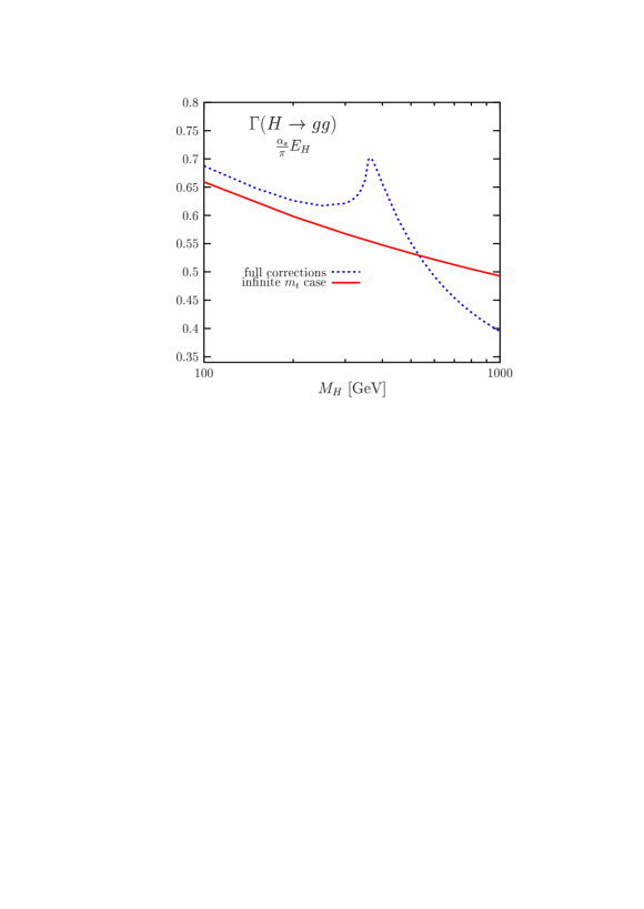
Figure 12: The QCD correction factor for the partial width $\Gamma(H\rightarrow gg)$ as a function of the Higgs boson mass, in the full massive case with $m_{t}\!=\!178$ GeV (dotted line) and in the heavy-top-quark limit (solid line). The strong coupling constant is normalized at $\alpha_{s}(M_{Z})\!=\!0.118$. From Ref. Djouadi:2005gi .

We also observe that the first order of QCD corrections has quite a large impact on the lowest order cross section, amounting to more than 50% of $\Gamma_{LO}$ on average. This has been indeed the main reason to prompt for a NNLO QCD calculation of $\Gamma(H\rightarrow gg)$. The result, obtained in the heavy-top approximation, has shown that NNLO QCD corrections amount to only 20% of the NLO cross section, therefore pointing to a convergence of the $\Gamma(H\rightarrow gg)$ perturbative series. We will refer to this discussion when dealing with the $gg\rightarrow H$ production mode, since its cross section can be easily related to $\Gamma(H\rightarrow gg)$.

III.2 MSSM Higgs boson branching ratios

The decay patterns of the MSSM Higgs bosons are many and diverse, depending on the specific choice of supersymmetric parameters. In particular they depend on the choice of $M_{A}$ and $\tan\beta$, which parameterize the MSSM Higgs sector, and they are clearly sensitive to the choice of other supersymmetric masses (gluino masses, squark masses, etc.) since this determines the possibility for the MSSM Higgs bosons to decay into pairs of supersymmetric particles and for the radiative induced decay channels ($h^{0},H^{0}\rightarrow gg,\gamma\gamma,\gamma Z$) to receive supersymmetric loop contributions.

Figure 13: Branching ratios for the $h^{0}$ and $H^{0}$ MSSM Higgs bosons, for $\tan\beta\!=\!3,30$. The range of $M_{H}$ corresponds to $M_{A}\!=\!90\,\mbox{GeV}-1\,\mbox{TeV}$, in the MSSM scenario discussed in the text, with maximal top-squark mixing. The vertical line in the left hand side plots indicates the upper bound on $M_{h}$, which, for the given scenario is $M_{h}^{max}\!=\!115$ GeV ($\tan\beta=3$) or $M_{h}^{max}\!=\!125.9$ GeV ($\tan\beta=30$). From Ref. Carena:2002es .

In order to be more specific, let us assume that all supersymmetric masses are large enough to prevent the decay of the MSSM Higgs bosons into pairs of supersymmetric particles (a good choice could be $M_{\tilde{g}}\!=\!M_{Q}\!=\!=\!M_{U}\!=\!M_{D}\!=\!1$ TeV). Then, we only need to examine the decays into SM particles and compare with the decay patterns of a SM Higgs boson to identify any interesting difference. From the study of the MSSM Higgs boson couplings in Sections II.4.3 and II.4.4, we expect that: i) in the decoupling regime, when $M_{A}\gg M_{Z}$, the properties of the $h^{0}$ neutral Higgs boson are very much the same as the SM Higgs boson; while away from the decoupling limit ii) the decay rates of $h^{0}$ and $H^{0}$ to electroweak gauge bosons are suppressed with respect to the SM case, in particular for large Higgs masses ($H^{0}$), iii) the $A^{0}\rightarrow VV$ ($V=W^{\pm},Z^{0}$) decays are absent, iv) the decay rates of $h^{0}$ and $H^{0}$ to $\tau^{+}\tau^{-}$ and $b\bar{b}$ are enhanced for large $\tan\beta$, v) even for not too large values of $\tan\beta$, due to ii) above, the $h^{0},H^{0}\rightarrow\tau^{+}\tau^{-}$ and $h^{0},H^{0}\rightarrow b\bar{b}$ decay are large up to the $t\bar{t}$ threshold, when the decay $H^{0}\rightarrow t\bar{t}$ becomes dominant, vi) for the charged Higgs boson, the decay $H^{+}\rightarrow\tau^{+}\nu_{\tau}$ dominates over $H^{+}\rightarrow t\bar{b}$ below the $t\bar{b}$ threshold, and vice versa above it.

As far as QCD and EW radiative corrections go, what we have seen in Sections III.1.2-III.1.4 for the SM case applies to the corresponding MSSM decays too. Moreover, the truly MSSM corrections discussed in Sections II.4.3 and II.4.4 need to be taken into account and are included in Figs.13 and 14.

Figure 14: Branching ratios for the $A^{0}$ and $H^{+}$ MSSM Higgs bosons, for $\tan\beta\!=\!3,30$. The range of $M_{H^{\pm}}$ corresponds to $M_{A}\!=\!90\,\mbox{GeV}-1\,\mbox{TeV}$, in the MSSM scenario discussed in the text, with maximal top-squark mixing. From Ref. Carena:2002es .

III.3 Direct bounds on both SM and MSSM Higgs bosons

LEP2 has searched for a SM Higgs at center of mass energies between 189 and 209 GeV. In this regime, a SM Higgs boson is produced mainly through Higgs boson strahlung from $Z$ gauge bosons, $e^{+}e^{-}\rightarrow Z^{*}\rightarrow HZ$, and to a lesser extent through $WW$ and $ZZ$ gauge boson fusion, $e^{+}e^{-}\rightarrow WW,ZZ\rightarrow H\nu_{e}\bar{\nu}_{e},He^{+}e^{-}$ (see Fig. 15). Once produced, it decays mainly into $b\bar{b}$ pairs, and more rarely into $\tau^{+}\tau^{-}$ pairs. The four LEP2 experiments have been looking for: i) a four jet final state ($H\rightarrow b\bar{b}$, $Z\rightarrow q\bar{q}$), ii) a missing energy final state ($H\rightarrow b\bar{b}$, $Z\rightarrow\nu\bar{\nu}$), iii) a leptonic final state ($H\rightarrow b\bar{b}$, $Z\rightarrow l^{+}l^{-}$) and iv) a specific $\tau$-lepton final state ($H\rightarrow b\bar{b}$, $Z\rightarrow\tau^{+}\tau^{-}$ plus $H\rightarrow\tau^{+}\tau^{-}$, $Z\rightarrow q\bar{q}$).

Figure 15: SM and MSSM neutral Higgs boson production channels at LEP2.

The absence of any statistical significant signal has set a 95% CL lower bound on the SM Higgs boson at

$$M_{H_{SM}}>114.4\,\,\mbox{GeV}\,\,\,.$$

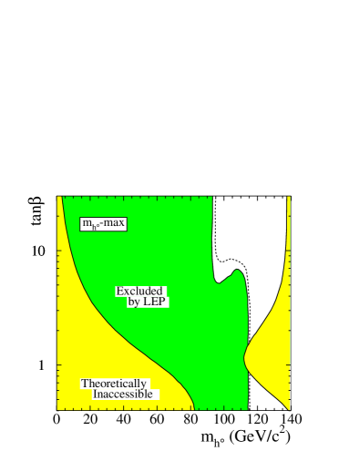
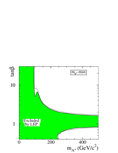
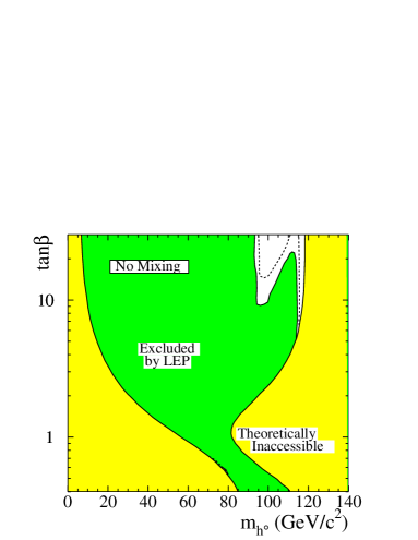
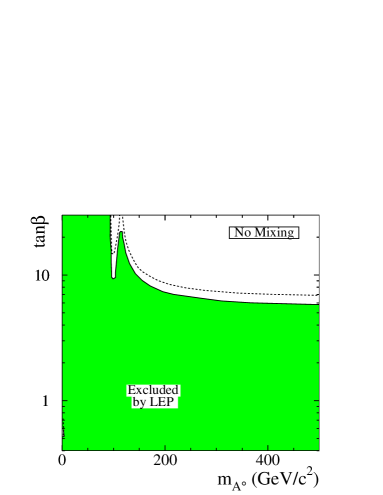
Figure 16: 95% CL exclusion limits for MSSM Higgs parameters from LEP2: $(M_{h},\tan\beta)$ (left) and $(M_{A},\tan\beta)$ (right). Both the maximal and no-mixing scenarios are illustrated, for $M_{S}\!=\!1$ TeV and $m_{t}\!=\!179.3$ GeV. The dashed lines indicate the boundaries that are excluded on the basis of Monte Carlo simulations in the absence of a signal. From Ref. Djouadi:2005gj .

LEP2 has also looked for the light scalar ($h^{0}$) and pseudoscalar ($A^{0}$) MSSM neutral Higgs bosons. In the decoupling regime, when $A^{0}$ is very heavy and $h^{0}$ behaves like a SM Higgs bosons, only $h^{0}$ can be observed and the same bounds established for the SM Higgs boson apply. The bound can however be lowered when $m_{A}$ is lighter. In that case, $h^{0}$ and $A^{0}$ can also be pair produced through $e^{+}e^{-}\rightarrow Z\rightarrow h^{0}A^{0}$ (see Fig. 15). Combining the different production channels one can derive plots like those shown in Fig. 16, where the excluded $(M_{h},\tan\beta)$ and $(M_{A},\tan\beta)$ regions of the MSSM parameter space are shown. The LEP2 collaborations lephwg:2004mssm have been able to set the following bounds at 95% CL:

$$M_{h,A}>93.0\,\,\mbox{GeV}\,\,\,,$$

obtained in the limit when $\cos(\beta-\alpha)\simeq 1$ (anti-decoupling regime) and for large $\tan\beta$. The plots in Fig. 16 have been obtained in the maximal mixing scenario (explained in Section II.4.2). For no-mixing, the corresponding plots would exclude a much larger region of the MSSM parameter space.

Finally, the LEP collaborations have looked for the production of the MSSM charged Higgs boson in the associated production channel: $e^{+}e^{-}\rightarrow\gamma,Z^{*}\rightarrow H^{+}H^{-}$ lhwg:2001xy . An absolute lower bound of

$$M_{H^{\pm}}>79.3\,\,\mbox{GeV}\,\,\,$$

has been set by the ALEPH collaboration, and slightly lower values have been obtained by the other LEP collaborations.

III.4 Higgs boson studies at the Tevatron and at the LHC

The parton level processes through which a SM Higgs boson can be produced at hadron colliders are illustrated in Figs. 17 and 18.

Figure 17: Leading Higgs production processes at hadron colliders: $gg\rightarrow H$, $qq\rightarrow qqH$, and $q\bar{q}\rightarrow WH,ZH$.

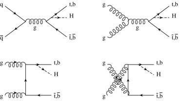
Figure 18: Higgs production with heavy quarks: sample of Feynman diagrams illustrating the two corresponding parton level processes $q\bar{q},gg\rightarrow t\bar{t}H,b\bar{b}H$. Analogous diagrams with the Higgs boson leg attached to the remaining top(bottom)-quark legs are understood.

Figures 19 and 20 summarize the cross sections for all these production modes as functions of the SM Higgs boson mass, at the Tevatron (center of mass energy: $\sqrt{s}\!=\!1.96$ TeV) and at the LHC (center of mass energy: $\sqrt{s}\!=\!14$ TeV). These figures have been recently produced during the TeV4LHC workshop Tev4lhc:hwg , and contain all known orders of QCD corrections as well as the most up to date input parameters. We postpone further details about QCD corrections till Section IV, while we comment here about some general phenomenological aspects of hadronic Higgs production.

The leading production mode is gluon-gluon fusion, $gg\rightarrow H$ (see first diagram in Fig. 17). In spite of being a loop induced process, it is greatly enhanced by the top-quark loop. For light and intermediate mass Higgs bosons, however, the very large cross section of this process has to compete against a very large hadronic background, since the Higgs boson mainly decays to $b\bar{b}$ pairs, and there is no other non-hadronic probe that can help distinguishing this mode from the overall hadronic activity in the detector. To beat the background, one has often to employ subleading if not rare Higgs decay modes, like $H\rightarrow\gamma\gamma$, and this dilutes the large cross section. For larger Higgs masses, above the $ZZ$ threshold, on the other hand, gluon-gluon fusion together with $H\rightarrow ZZ$ produces a very distinctive signal, and make this mode a “gold-plated mode” for detection. For this reason, $gg\rightarrow H$ plays a fundamental role at the LHC over the entire Higgs boson mass range, but is of very limited use at the Tevatron, where it can only be considered for Higgs boson masses very close to the upper reach of the machine ($M_{H}\simeq 200$ GeV).

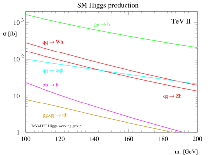
Figure 19: Cross sections for SM Higgs boson production processes at the Tevatron, Run II ($\sqrt{s}\!=\!1.96$ TeV). From Ref. Tev4lhc:hwg .

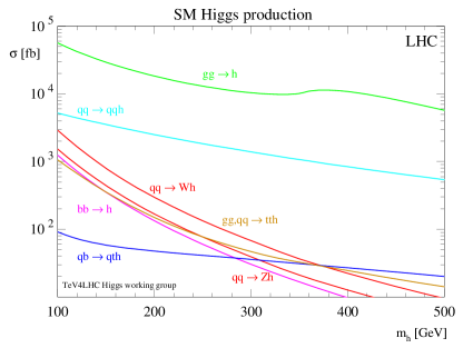
Figure 20: Cross sections for SM Higgs boson production processes at the LHC ($\sqrt{s}\!=\!14$ TeV). From Ref. Tev4lhc:hwg .

Weak boson fusion ($qq\rightarrow qqH$, see second diagram in Fig. 17) and the associated production with weak gauge bosons ($q\bar{q}\rightarrow WH,ZH$, see third diagram in Fig. 17) have also fairly large cross sections, of different relative size at the Tevatron and at the LHC. $q\bar{q}\rightarrow WH,ZH$ is particularly important at the Tevatron, where only a relatively light Higgs boson ($M_{H}<200$ GeV) will be accessible. In this mass region, $gg\rightarrow H,H\rightarrow\gamma\gamma$ is too small and $qq\rightarrow qqH$ is suppressed (because the initial state is $p\bar{p}$). On the other hand, $qq\rightarrow qqH$ becomes instrumental at the LHC ($pp$ initial state) for low and intermediate mass SM Higgs bosons, where its characteristic final state configuration, with two very forward jets, has been shown to greatly help in disentangling this signal from the hadronic background, using different Higgs decay channels.

Finally, the production of a SM Higgs boson with heavy quarks, in the two channels $q\bar{q},gg\rightarrow Q\bar{Q}H$ (with $Q\!=\!t,b$, see Fig. 18), is sub-leading at both the Tevatron and the LHC, but has a great physics potential. The associated production with $t\bar{t}$ pairs is probably too small to be seen at the Tevatron, given the expected luminosities, but will play a very important role for a light SM Higgs boson ($M_{H}\!<\!130-140$ GeV) at the LHC, where enough statistics will be available to fully exploit the spectacular signature of a $t\bar{t}H,H\rightarrow b\bar{b}$ final state. Moreover, at the LHC, the associated production of a Higgs boson with top quarks will offer a direct handle on the top-quark Yukawa coupling (see Section III.4.2). On the other hand, the production of a SM Higgs boson with $b\bar{b}$ pairs is tiny, since the SM bottom-quark Yukawa coupling is suppressed by the bottom-quark mass. Therefore, the $b\bar{b}H,\,H\rightarrow b\bar{b}$ channel is the ideal candidate to provide evidence of new physics, in particular of extension of the SM, like supersymmetric models, where the bottom-quark Yukawa coupling to one or more Higgs bosons is enhanced (e.g., by large $\tan\beta$ in the MSSM). $b\bar{b}H$ production is kinematically well within the reach of the Tevatron, RUN II. First studies from both CDF Affolder:2000rg and D$\emptyset$ Abazov:2005yr have already translated the absence of a $b\bar{b}h^{0},H^{0},A^{0}$ signal into an upper bound on the $\tan\beta$ parameter of the MSSM. Were a signal observed, $b\bar{b}H$ could actually provide the first piece of evidence for new physics from RUN II.

III.4.1 Searching for a SM Higgs boson at the Tevatron and the LHC

Discovering a Higgs boson during RUN II of the Tevatron is definitely among the most important goal of this collider. It will be challenging and mainly luminosity limited, but recent studies have confirmed that RUN II can push the 95% CL exclusion limit much farer than LEP2 and also shoot for a $3\sigma$ or $5\sigma$ discovery, depending on the integrated luminosity accumulated.

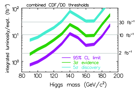
Figure 21: Integrated luminosity required for each experiment at the Tevatron, Run II, to exclude a SM Higgs boson at 95% CL or to observe it at the $3\sigma$ or $5\sigma$ level. Original study from Ref. Carena:2000yx .

The plot in Fig. 21 shows the integrated luminosity that was originally estimated to be necessary to reach the 95% CL exclusion limit, the $3\sigma$, and the $5\sigma$ discovery levels. It is given for a SM Higgs boson mass up to 200 GeV, that is to be considered as the highest Higgs boson mass reachable by RUN II. The curves have been obtained mainly by using the associated production with weak gauge bosons, $q\bar{q}\rightarrow VH$ ($V\!=\!W^{\pm},Z^{0}$), with $H\rightarrow b\bar{b}$ and $H\rightarrow W^{+}W^{-}$, over the entire Higgs boson mass range, and $gg\rightarrow H$ with $H\rightarrow ZZ$ in the upper mass region. As discussed in the introduction to Section III.4, this can be understood in terms of production cross sections (see Fig. 19) and decay branching ratios (see Fig. 9) over the $M_{H}\!=\!115-200$ GeV mass range. From Fig. 21 we see that with, e.g., 10 fb^-1 of integrated luminosity RUN II will be able to put a 95% CL exclusion limit on a SM Higgs boson of mass up to $180$ GeV, while it could claim a $3\sigma$ discovery of a SM Higgs boson with mass up to $125$ GeV. A $5\sigma$ discovery of a SM Higgs boson up to 130 GeV, i.e. in the region immediately above the LEP2 lower bound, seemed to require 30 fb^-1 of integrated luminosity, well beyond what is currently expected for RUN II.

More recently, a new sensitivity study has appeared Babukhadia:2003zu , where the low mass region only has been revisited and new luminosity curves have been drawn. Mainly using the $q\bar{q}\rightarrow VH$ ($V\!=\!W^{\pm},Z^{0}$) production mode, it appears that new analyses techniques will allow to obtain better results with less integrated luminosity. A $3\sigma$ discovery of a SM Higgs boson with mass up to $125$ GeV will now require only about 5 fb^-1, while 10 fb^-1 could allow a $5\sigma$ discovery of a SM Higgs boson with mass up to about $120$ GeV, right at the LEP2 lower bound limit.

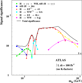
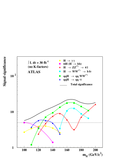
Figure 22: Significance for the SM Higgs boson discovery in various detection channels as a function of $M_{H}$. The upper plot is for 100 fb^-1 of data and with no $qqH$ channel included, the lower plot for 30 fb^-1 and with the $qqH$ channel included over the mass range $M_{H}\!<\!200$ GeV. Results are from the ATLAS collaboration atlas:asai_etal .

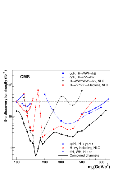
Figure 23: Luminosity required to reach a $5\sigma$ discovery signal in CMS, using various detection channels, as a function of $M_{H}$. From Ref. cms:abdullin_etal .

At the LHC, all production modes will play an important role, thanks to the higher statistics available. In particular, it is natural to distinguish between a light ($M_{H}\!<\!130-140$ GeV) and heavy ($M_{H}>130-140$ GeV) mass region, as becomes evident by simultaneously looking at both production cross sections (see Fig. 20) and decay branching ratios (see Fig. 9) over the entire $115-1000$ GeV SM Higgs boson mass range. In the region of $M_{H}\!<\!130-140$ GeV the SM Higgs boson at the LHC will be searched mainly in the following channels:

$$gg\rightarrow H\,,\,H\rightarrow\gamma\gamma,W^{+}W^{-},ZZ\,\,\,,$$ (116)

$$qq\rightarrow qqH\,,\,H\rightarrow\gamma\gamma,W^{+}W^{-},ZZ,\tau^{+}\tau^{-}\,\,\,,$$

$$q\bar{q},gg\rightarrow t\bar{t}H\,,\,H\rightarrow b\bar{b},\tau^{+}\tau^{-}\,\,\,,$$

while above that region, i.e. for $M_{H}\!>\!130-140$ GeV, the discovery modes will be:

$$gg\rightarrow H\,,\,H\rightarrow W^{+}W^{-},ZZ\,\,\,,$$ (117)

$$qq\rightarrow qqH\,,\,H\rightarrow\gamma\gamma,W^{+}W^{-},ZZ\,\,\,,$$

$$q\bar{q},gg\rightarrow t\bar{t}H\,,\,H\rightarrow W^{+}W^{-}\,\,\,.$$

These have been the modes used by both ATLAS and CMS to provide us with the discovery reach illustrated in Figs. 22 and 23. The ATLAS plots give the signal significance for a total integrated luminosity of 100 fb^-1 (upper plot) and of 30 fb^-1 (lower plot). The high luminosity (upper) plot belongs to the original ATLAS technical design report atlas:1999tdr , and the weak boson fusion channels had not been studied in detail at that time. The lower luminosity (lower) plot is taken from a more updated study atlas:asai_etal , and the weak boson fusion channels have been included in the low mass region, up to about $M_{H}\!\simeq\!200$ GeV, where they play an instrumental role towards discovery. Other instrumental channels in the low mass region are the inclusive Higgs production with $H\rightarrow\gamma\gamma$ and, below $M_{H}\!=\!130$ GeV, $t\bar{t}H$ production with $H\rightarrow b\bar{b}$. In the high mass region, the inclusive production with $H\rightarrow ZZ,WW$ dominates, although CMS has found a substantial contribution coming from weak gauge boson fusion with $H\rightarrow ZZ,WW$.

III.4.2 Studies of a SM Higgs boson

If a Higgs boson signal is established, the LHC will have the capacity of measuring several of its properties at some level of accuracy. In particular, it will be able to measure its mass, width, and couplings. At the same time, the charge and color quantum numbers of the newly discovered particle will be established by detecting a single production-decay channel; while a precise determination of its spin and parity will probably require more statistics than available at the LHC and will have to wait for a high energy Linear Collider to be established (see Section III.5).

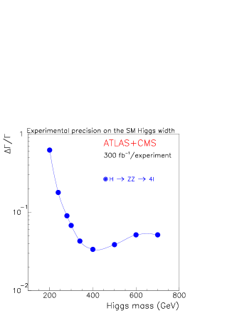
Figure 24: Expected precision in the measurement of a SM-like Higgs boson mass ($M_{H}$) and width ($\Gamma_{H}$) combining 300 fb^-1 of data per experiment from ATLAS and CMS. From Ref. Gianotti:2000tz .

The two plots in Fig. 24 show the precision with which both the mass and width of a SM-like Higgs boson will be determined by ATLAS and CMS combining 300 fb^-1 of data per experiment. We see that below $M_{H}\!\simeq\!400$ GeV the Higgs mass can be determined with a precision of about 0.1%, through $H\rightarrow ZZ\rightarrow 4l$, complemented by $H,WH,t\bar{t}H(H\rightarrow\gamma\gamma)$ and $t\bar{t}H(H\rightarrow b\bar{b})$ in the low mass region. Above $M_{H}\!\simeq\!400$ GeV the accuracy deteriorates for the smaller statistics available, although precisions of the order of 1% can still be obtained. We also see that the Higgs width above $M_{H}\!\simeq\!200$ GeV will be entirely determined through $H\rightarrow ZZ\rightarrow 4l$, while below $M_{H}\!\simeq\!200$ GeV it is too small to be resolved experimentally and can only be determined indirectly, as we will discuss in the following.

Finally, many studies in recent years have pointed to the fact that the LHC, under minimal theoretical assumptions, will have the potential to measure several Higgs boson couplings with an accuracy in the 10-30% range. The proposed strategy Zeppenfeld:2000td consists of measuring the production-decay channels listed in Eqs. (116) and (117) for a light ($M_{H}\!\leq\!130-140$ GeV) or heavy ($M_{H}\!\geq\!130-140$ GeV) Higgs boson respectively, and combine them to extract individual partial widths or ratios of partial widths. Indeed, if a given production-decay channel is observed, one can write that the experimentally measured product of production cross section times decay branching ratio corresponds, in the narrow width approximation, to the following expression:

$$(\sigma_{p}(H)\mathrm{Br}(H\rightarrow dd))^{exp}=\frac{\sigma_{p}^{th}(H)}{\Gamma^{th}_{p}}\frac{\Gamma_{d}\Gamma_{p}}{\Gamma}\,\,\,,$$ (118)

where $\Gamma_{p}$ and $\Gamma_{d}$ are the partial widths associated with the production and decay channels respectively, while $\Gamma$ is the Higgs boson total width. The coefficient $\sigma_{p}^{th}(H)/\Gamma^{th}_{p}$ can be calculated, while $\Gamma_{p}$, $\Gamma_{d}$, and $\Gamma$ is what needs to be determined. To each production-decay channel one can therefore associate a measurable observable

$$Z^{(p)}_{d}=\frac{\Gamma_{p}\Gamma_{d}}{\Gamma}\,\,\,,$$ (119)

where $p$ and $d$ label the production and decay channels respectively. $Z^{(p)}_{d}$ is obtained from the experimental measurement of $(\sigma_{p}(H)\mathrm{Br}(H\rightarrow dd))^{exp}$, normalized by the theoretically calculable coefficient $\sigma_{p}^{th}(H)/\Gamma^{th}_{p}$. A signal in the $(p,d)$ channel will measure $Z^{(p)}_{d}$, and therefore the product of Higgs couplings $y_{p}^{2}y_{d}^{2}$, since $\Gamma_{p}\simeq y_{p}^{2}$ and $\Gamma_{d}\simeq y_{d}^{2}$. Combining many different $(p,d)$ channels, a system of equations of the form of Eq. (119) is obtained. Ratios of partial widths $\Gamma_{i}/\Gamma_{j}$, and therefore ratios of Higgs couplings, can then be derived in a model independent way, e.g.:

$$\frac{\Gamma_{b}}{\Gamma_{\tau}} = \frac{Z^{(t)}_{b}}{Z^{(t)}_{\tau}}\longrightarrow\frac{y_{b}}{y_{\tau}}\,\,\,,$$ (120)

$$\frac{\Gamma_{t}}{\Gamma_{g}} = \frac{Z^{(t)}_{\tau}Z^{(w)}_{\gamma}}{Z^{(w)}_{\tau}Z^{(g)}_{\gamma}}\longrightarrow\frac{y_{t}}{y_{g}}\,\,\,,$$

while individual partial width can be obtained with the further assumptions that: i) the total width is the sum of all SM partial widths, i.e. there is no new physics or invisible width contributions, and ii) the $y_{W}$ and $y_{Z}$ couplings are related by the $SU(2)_{L}$ weak isospin symmetry. This is required by the fact that, in $qq\rightarrow qqH$, the $W^{+}W^{-}\rightarrow H$ and $ZZ\rightarrow H$ fusion processes cannot be distinguished experimentally.

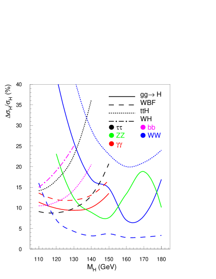
Figure 25: Relative accuracies on the measurement of the cross section of a scalar SM-like Higgs boson in the production+decay channels listed in Eqs. (116) and (117). All channels have been rescaled to a total integrated luminosity of 200 fb^-1, except $pp\rightarrow t\bar{t}H,H\rightarrow W^{+}W^{-}$ and $q\bar{q}\rightarrow WH,H\rightarrow b\bar{b}$ for which 300  fb^-1 have been used, and $gg\rightarrow H,H\rightarrow W^{+}W^{-}$ that was studies with 30 fb^-1. From Ref. Belyaev:2002ua .

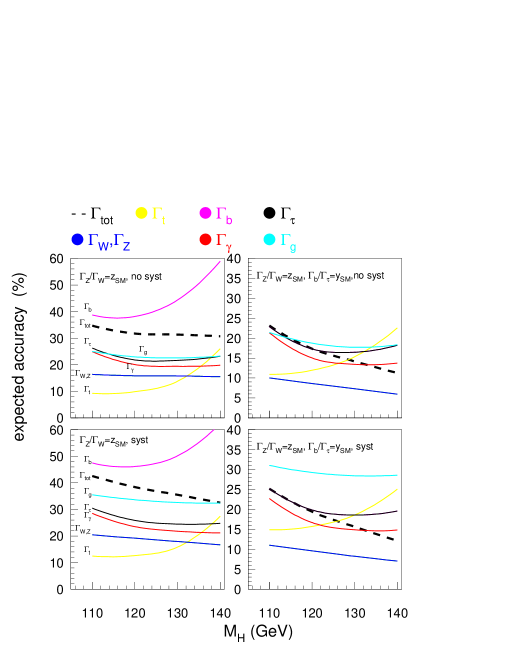
Figure 26: Relative accuracy on the individual rates $\Gamma_{i}$ expected at the LHC, when the ratio $\Gamma_{b}/\Gamma_{\tau}$ is fixed to its SM value (right plots) or not (left plots). The integrated luminosity used is as explained in the caption of Fig. 25. The upper plots show the accuracies obtained without including any theoretical systematic error, while the lower plots include the systematic theoretical errors explained in the text. From Ref. Belyaev:2002ua .

The accuracy with which both individual couplings and ratios of couplings can be extracted is mainly determined by the experimental error on the $Z^{(p)}_{d}$ measurements and by the theoretical uncertainty on the prediction of $\sigma_{p}^{th}(H)$ in Eq. (118). Fig. 25 shows the estimated relative accuracy with which various channel will be detected at the LHC, assuming 200 fb^-1 of data available for most channels. For the purpose of illustration, Fig. 26 shows the accuracy with which some of the SM Higgs partial width as well as its total width could be determined at the LHC, when the technique described above is implemented. The upper plots do not include any theoretical systematic error, while the lower plots include a theoretical systematic error of: 20% for $gg\rightarrow H$, 5% for $qq\rightarrow qqH$, and 10% for $pp\rightarrow t\bar{t}H$. At the same time, all plots assumes the $SU(2)$ gauge induced relation between $y_{W}$ and $y_{Z}$, while the right hand plots also assume a SM-like relation between $y_{b}$ and $y_{\tau}$. The more the assumptions, the better the accuracy with which the considered couplings can be determined, and the more model dependence is introduced in the coupling determination. More sophisticated analyses have appeared in recent studies Assamagan:2004mu ; Duhrssen:2004cv . Overall, we can however conclude that the LHC has a great potential of giving a first fairly precise indication of the nature of the couplings of a Higgs boson candidate, although under some (well justified) model assumptions. In particular, in the specific case of the top-quark Yukawa coupling, the LHC will be for a long time the only machine to be able to measure it with enough precision, since the measurement of $y_{t}$ in $e^{+}e^{-}\rightarrow t\bar{t}H$ at a $\sqrt{s}\!=\!500$ GeV Linear Collider is statistically very limited, as we will see in Section III.5.

III.4.3 Searching for a MSSM Higgs boson at the Tevatron and the LHC

Most of the characteristics of the MSSM Higgs couplings that determine the pattern of decays reviewed in Section III.2 also affect the mechanism of production of the MSSM Higgs bosons. In particular:

• for $M_{A}\gg M_{Z}$, the so called decoupling limit,

  • $h^{0}\longrightarrow H_{SM}$, while

  • $M_{A}\simeq M_{H}\,\,\,$ and $\,\,\,g_{(A,H)b\bar{b}}\gg g_{H_{SM}b\bar{b}}\,\,\,$, $\,\,\,g_{HVV}\ll g_{H_{SM}VV}$,

• while for $M_{A}\leq M_{Z}$ and $\tan\beta\gg 1$:

  • $g_{HVV}\simeq g_{H_{SM}VV}$, while

  • $M_{A}\simeq M_{h}\,\,\,$ and $\,\,\,g_{(A,h)b\bar{b}}\gg g_{H_{SM}b\bar{b}}\,\,\,$, $\,\,\,g_{hVV}\ll g_{H_{SM}VV}$.

If we assume supersymmetric particles to be heavy enough that the decay of a Higgs boson into supersymmetric particles as well as the production of a Higgs boson through the decay of a supersymmetric particle is forbidden, the available production processes are the SM ones plus the associate production modes illustrated in Fig. 27, as well as the production of a charged Higgs boson via the decay of a $t/\bar{t}$ quark.

Figure 27: Associated production modes for MSSM Higgs bosons.

A summary of the neutral MSSM Higgs boson production rates at the Tevatron and at the LHC is given in Figs. 28 and 29, for two values of $\tan\beta$, in the maximal mixing scenario (see Section II.4.2). For the Tevatron the mass range is limited to the range kinematically accessible while for the LHC the entire Higgs mass range up to 1 TeV is covered. It is important to notice how for large $\tan\beta$ ($\tan\beta\!=\!30$ in the plots of Figs. 28 and 29) the production of both scalar and pseudoscalar neutral Higgs boson with bottom quarks becomes dominant. In particular the inclusive production (denoted in the Figs. 28 and 29 as $b\bar{b}\rightarrow\phi^{0}$, for $\phi^{0}\!=\!h^{0},H^{0},A^{0}$) becomes larger than the otherwise dominant gluon-gluon fusion mode ($gg\rightarrow H$), while the exclusive production (denoted in Figs. 28 and 29 as $p\bar{p},pp\rightarrow b\bar{b}\phi^{0}$) is right below gluon-gluon fusion but above all other production modes. More details on exclusive vs inclusive production of a Higgs boson with bottom quarks will be given in Section IV. We also notice the subleading role played by vector boson fusion production ($qq\rightarrow qq\phi^{0}$) due to the suppression (or absence in the case of $A^{0}$) of the $\phi^{0}VV$ couplings (for $V\!=\!W^{\pm},Z$). Finally, the associated production modes for neutral Higgs bosons (see Fig. 27) have in general very small cross sections and are not considered in the plots of Figs. 28 and 29.

Figure 28: Neutral MSSM Higgs boson cross sections at the Tevatron ($\sqrt{s}\!=\!2$ TeV). The upper plots are for the neutral scalar Higgs bosons, $h^{0}$ and $H^{0}$, while the lower plots are for the neutral pseudoscalar Higgs boson, $A^{0}$. The left hand plots are for $\tan\beta\!=\!3$ while the right hand plots are for $\tan\beta\!=\!30$. From Ref. Carena:2002es .

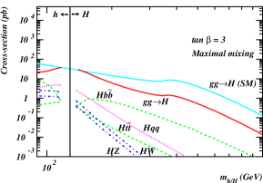
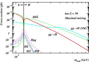
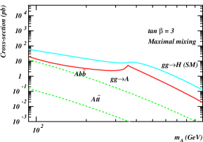
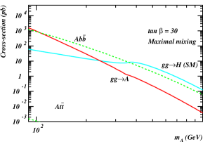
Figure 29: Neutral MSSM Higgs boson cross sections at the LHC ($\sqrt{s}\!=\!14$ TeV). The upper hand plots are for the neutral scalar Higgs bosons, $h^{0}$ and $H^{0}$, while the lower plots are for the neutral pseudoscalar Higgs boson, $A^{0}$. The left hand plots are for $\tan\beta\!=\!3$ while the right hand plots are for $\tan\beta\!=\!30$. From Ref. Carena:2002es .

For the case of the charged MSSM Higgs boson, we need to distinguish two cases: i) $M_{H^{\pm}}<m_{t}-m_{b}$ and ii) $M_{H^{\pm}}>m_{t}-m_{b}$. When $M_{H^{\pm}}<m_{t}-m_{b}$, $H^{\pm}$ is mainly produced via the decay of a top or anti-top in $t\bar{t}$ production, i.e. via $p\bar{p},pp\rightarrow t\bar{t}$ with $t\rightarrow bH^{+}$ or $\bar{t}\rightarrow\bar{b}H^{-}$. On the other hand, when $M_{H^{\pm}}>m_{t}-m_{b}$, $H^{\pm}$ is mainly produced through $p\bar{p}\rightarrow\bar{t}bH^{+},t\bar{b}H^{-}$, as well as through the tree level production modes $q\bar{q}\rightarrow H^{+}H^{-}$ and $b\bar{b}\rightarrow W^{\pm}H^{\mp}$, and at one loop through the associated modes $gg\rightarrow H^{+}H^{-}$ and $gg\rightarrow W^{\pm}H^{\mp}$. The overall cross section for the Tevatron and the LHC is illustrated in Figs. 30 and 31 as a function of the charged Higgs boson mass, for different values of $\tan\beta$. The threshold behavior at $M_{H}^{\pm}\simeq m_{t}-m_{b}$ is clearly visible.

Figure 30: Charged Higgs boson cross sections at the Tevatron, as a function of $M_{H^{\pm}}$, for different values of $\tan\beta$. From Ref. Carena:2002es .

Figure 31: Charged Higgs boson cross sections at the LHC as functions of $M_{H^{\pm}}$, for different values of $\tan\beta$. From Ref. Carena:2002es .

The evidence or the absence of evidence for an MSSM Higgs boson at the Tevatron or at the LHC will place definite bounds on the parameter space of the MSSM. The reach of the Tevatron in the $(M_{A},\tan\beta)$ plane is illustrated in Fig. 32 for different integrated luminosities. The shaded regions are spanned by using only the $q\bar{q}\rightarrow V\phi^{0}\,\,(\phi^{0}\rightarrow b\bar{b})$ channel (with $\phi^{0}=h^{0},H^{0}$), while the region above the solid curves are covered by using the $gg,q\bar{q}\rightarrow b\bar{b}\phi^{0}\,\,(\phi^{0}\rightarrow b\bar{b})$ channel (with $\phi^{0}=h^{0},H^{0},A^{0}$). The region below the black solid line is excluded by searches at LEP2. Fig. 32 shows that, although discovery may require integrated luminosities that are beyond the reach of RUN2 of the Tevatron, with 5 fb^-1 CDF and D$\emptyset$ will be able to exclude (in the maximal mixing scenario) almost all the parameter space of the MSSM at 95% C.L., a pretty impressive result by itself!

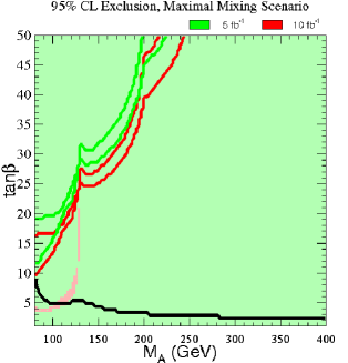
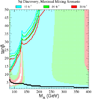
Figure 32: 95% C.L. exclusion region and $5\sigma$ discovery region in the $(M_{A},\tan\beta)$ plane, for the maximal mixing scenario. The shaded regions correspond to the search channel $q\bar{q}\rightarrow V\phi^{0}\,\,(\phi^{0}\rightarrow b\bar{b})$ (with $\phi^{0}=h^{0},H^{0}$), while the regions delimited by the colored solid lines correspond to the search channel $gg,q\bar{q}\rightarrow b\bar{b}\phi^{0}\,\,(\phi^{0}\rightarrow b\bar{b})$ (with $\phi^{0}=h^{0},H^{0},A^{0}$). The two sets of lines correspond to simulations from CDF and D$\emptyset$ respectively. The region below the black line has been excluded by searches at LEP2. From Ref. Carena:2002es . See also Ref. Carena:2000yx .

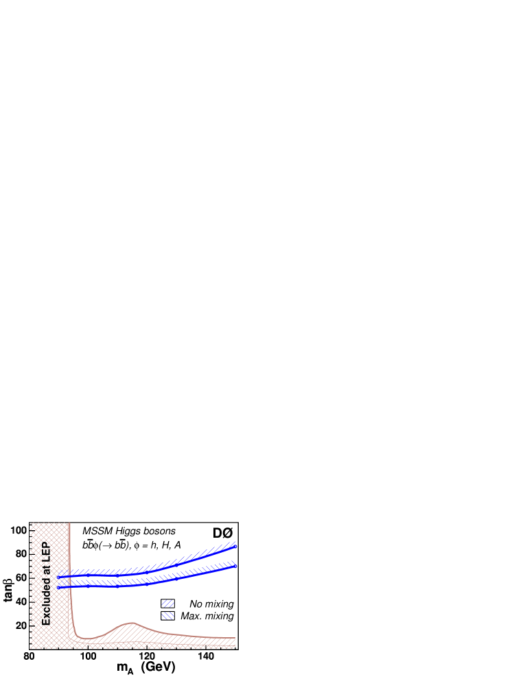
Figure 33: The 95% C.L. upper limit on $\tan\beta$ as a function of $M_{A}$ for two scenarios of the MSSM, no mixing and maximal mixing. Also shown are the limits obtained by the LEP experiments for the same two scenarios of the MSSM. From Ref. Abazov:2005yr , D$\emptyset$ analysis based on 260 pb^-1 of data. .

Both CDF and D$\emptyset$ have indeed already presented results from searches conducted in the $p\bar{p}\rightarrow b\bar{b}\phi^{0}\,\,(\phi^{0}\rightarrow b\bar{b})$ channel with three or four $b$-quark jets tagged in the final state Abazov:2005yr . The most recent results, from D$\emptyset$, are illustrated in Fig. 33, where we can see that, depending on $M_{A}$, values of $\tan\beta$ as low as $\tan\beta\!=\!50$ have already been excluded.

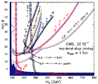
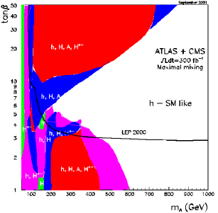
Figure 34: $5\sigma$ discovery contours for MSSM Higgs boson detection in various channels, shown in the $(M_{A},\tan\beta)$ parameter space, assuming the maximal mixing scenario. The left hand plot is from the CMS experiment and assumes 30 fb^-1 of integrated luminosity, while the right hand plot combines ATLAS and CMS with a total integrated luminosity of 300 fb^-1.

The LHC $5\sigma$ discovery reach in the $(M_{A},\tan\beta)$ parameter space is illustrated in Fig. 34. Thanks to the high luminosity available and to the complementarity of various production and decay modes, the entire $(M_{A},\tan\beta)$ parameter space can be covered, up to $M_{A}$ of the order of 1 TeV. This gives us the exciting perspective that the LHC will be able to either discover or completely rule out the existence of an MSSM Higgs boson!

III.5 Higgs boson studies at a future $e^{+}e^{-}$ Linear Collider

As we all know, an $e^{+}e^{-}$ collider provides a very clean environment, with relatively simple signatures and very favorable signal to background ratios. Therefore, one of the most important roles that a high energy $e^{+}e^{-}$ collider (to which we will refer as International Linear Collider (ILC) or simply Linear Collider (LC)) will play is to unambiguously identify any new particle discovered at the Tevatron or at the LHC, through a thorough program of precision measurements. This is true in Higgs boson physics as well, where we expect the mass, width, spin, and couplings of any Higgs boson candidates to be determined at the few percent level. In this Section I will mainly focus on a SM Higgs boson, since this is enough to illustrate the role played by a LC in Higgs physics, and since the true impact on the study of the MSSM parameter space will be shaped by the discoveries occured by the time a LC is built.

First of all, the most important SM Higgs boson production processes in $e^{+}e^{-}$ collisions are illustrated in Figs. 35 and 36 and are: i) $e^{+}e^{-}\rightarrow ZH$, the Higgs strahlung or associated production with $Z$ gauge bosons, ii) $e^{+}e^{-}\rightarrow H\nu\bar{\nu}$, the $W^{+}W^{-}$ fusion production, and $e^{+}e^{-}\rightarrow He^{+}e^{-}$, the $ZZ$ fusion production, iii) $e^{+}e^{-}\rightarrow t\bar{t}H$, the associated production with a $t\bar{t}$ pair. In addition, in the MSSM we also have: iv) $e^{+}e^{-}\rightarrow h^{0}A^{0},H^{0}A^{0}$ and $e^{+}e^{-}\rightarrow H^{+}H^{-}$, the pair production of two Higgs bosons, either neutral or charged, as illustrated in Fig. 37.

Figure 35: Higgs boson production via Higgs strahlung and $W^{+}W^{-},ZZ$ fusion at $e^{+}e^{-}$ colliders.

Figure 36: Higgs boson production in association with $t\bar{t}$ pairs at $e^{+}e^{-}$ colliders.

Figure 37: MSSM Higgs pair production at $e^{+}e^{-}$ colliders.

The cross sections of these processes as functions of the corresponding Higgs masses are illustrated in Figs. 38 and 39 for various center of mass energies ($\sqrt{s}$).

Figure 38: SM Higgs boson production cross sections in $e^{+}e^{-}$ collisions, for various center of mass energies ($\sqrt{s}$). From Ref. Aguilar-Saavedra:2001rg .

Figure 39: MSSM Higgs boson production cross sections in $e^{+}e^{-}$ collisions, for two choices of $\tan\beta$: $\tan\beta\!=\!3$ (solid) $\tan\beta\!=\!30$ (dotted), at $\sqrt{s}\!=\!350$ GeV, for $h^{0}$ and $H^{0}$, and at $\sqrt{s}\!=\!800$ GeV, for $A^{0}$ and $H^{\pm}$. From Ref. Aguilar-Saavedra:2001rg .

$e^{+}e^{-}\rightarrow ZH$ and $e^{+}e^{-}\rightarrow H\nu\bar{\nu}$ are the leading production modes for a SM Higgs bosons. Their relative size varies with the center of mass energy, since $\sigma(e^{+}e^{-}\rightarrow ZH)$ scales as $1/s$ ($s$-channel process), while $\sigma(e^{+}e^{-}\rightarrow H\nu\bar{\nu})$ scales as $\log(s)$ ($t$-channel process). $e^{+}e^{-}\rightarrow H\nu\bar{\nu}$ always dominates over $e^{+}e^{-}\rightarrow He^{+}e^{-}$ by almost one order of magnitude. In the MSSM, $e^{+}e^{-}\rightarrow H\nu\bar{\nu}$ plays a lesser role, due to the suppression of the $VVH$ coupling ($V\!=\!W^{\pm},Z$), but the $h^{0}A^{0}$, $H^{0}A^{0}$ and $H^{+}H^{-}$ pair production modes become important. $t\bar{t}H$ production is always very rare, in particular at center of mass energies around 500 GeV or lower, but it plays a really important role at higher energies, around 800 GeV-1 TeV, for the determination of the top-quark Yukawa coupling, as we will discuss later. Other rare production modes that could play an important role in determining some Higgs boson properties are the double Higgs boson production modes: $e^{+}e^{-}\rightarrow HHZ$ and $e^{+}e^{-}\rightarrow HH\nu\bar{\nu}$

With a LC running at energies between 350 GeV and 1 TeV, one or more Higgs bosons can be observed over the entire mass spectrum and all its properties can be precisely studied. Reconstructing the recoiling $l^{+}l^{-}$ mass (for $l\!=\!e,\mu$) in $e^{+}e^{-}\rightarrow HZ\rightarrow Hl^{+}l^{-}$, where the $Z$ is mono-energetic, allows an excellent and model independent determination of the Higgs boson mass. $Z\rightarrow q\bar{q}$ decays can also be used and actually provide a very large statistics. Accuracies of the order of 50-80 MeV can be obtained, depending on the center of mass energy and the Higgs boson mass. The spin and parity of the Higgs boson candidate (expected to be $J^{P}\!=\!0^{+}$) can be determined in several ways, among others: i) from the onset of $\sigma(e^{+}e^{-}\rightarrow ZH)$, since the energy dependence near threshold strongly depend on the $J^{P}$ quantum number of the radiated $H$ (see Fig. 40); ii) from the angular distribution of $H$ and $Z$ in $e^{+}e^{-}\rightarrow ZH\rightarrow 4f$; iii) from the differential cross section in $e^{+}e^{-}\rightarrow t\bar{t}H$.

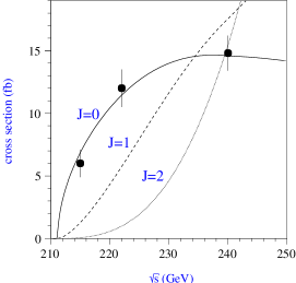
Figure 40: The $e^{+}e^{-}\rightarrow ZH$ cross section energy dependence near threshold for $M_{H}\!=\!120$ GeV and spin $J^{P}\!=\!0^{+},1^{-},2^{+}$. From Ref. Aguilar-Saavedra:2001rg .

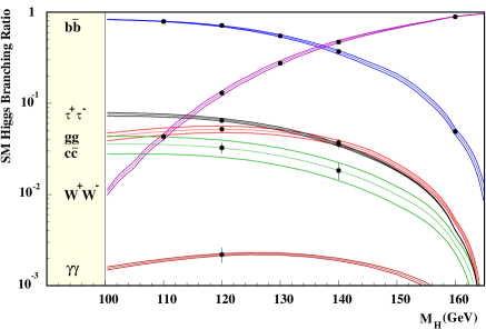
Figure 41: The theoretical predictions (bands, due to the uncertainty in the quark masses and $\alpha_{s}$) and experimental accuracies (dots with error bars) for the SM Higgs branching ratios at $\sqrt{s}\!=\!350$ GeV with 500 fb^-1 of data. From Ref. Aguilar-Saavedra:2001rg .

Finally, a high energy LC will measure the Higgs boson couplings to unprecedented precision and in a model independent way. Thanks to the precise knowledge of the initial state energy configuration (once the initial state radiation, or beam strahlung, has been properly taken into account), one can indeed measure both $\sigma(e^{+}e^{-}\rightarrow HZ\rightarrow Hl^{+}l^{-})$ and $\sigma(e^{+}e^{-}\rightarrow W^{*}W^{*}\nu\bar{\nu}\rightarrow H\nu\bar{\nu})$, reconstructing the mass recoiling against the $l^{+}l^{-}$ or $\nu\bar{\nu}$ pair, and from there determine in a model independent way the isolated $HZZ$ and $HWW$ couplings. This is probably the most important intrinsic difference between measuring the Higgs couplings at a lepton versus a hadron collider. At a lepton collider the Higgs couplings to the weak gauge bosons, i.e. the Higgs couplings associated to the production mode ($y_{p}$ of Section III.4.2), can be isolated in a model independent way. Any other coupling can then be also determined in a model independent way, measuring the individual $Br(H\rightarrow XX)$ in $e^{+}e^{-}\rightarrow HZ$ followed by $H\rightarrow XX$. Several recent studies have confirmed the possibility of determining Higgs couplings to both gauge boson and fermions within a few percent (2-5%). For instance, for a Higgs boson of $M_{H}\!=\!120$ GeV, the bottom-quark Yukawa coupling, $y_{b}$, could be determined within 2%, the $\tau$ one, $y_{\tau}$, within 5%, and the charm quark one, $y_{c}$ within 6% due to the larger error on the charm quark mass. This will test in a very stringent way the proportionality of the Higgs couplings to the mass of the interacting fermion. Even the indirect coupling of the Higgs boson to a pair of gluons, arising at the one-loop level (see Section. II.2), will be determined with a precision of 4-5%. This will allow an indirect check of the top-quark Yukawa coupling for a SM Higgs boson (when the top-quark loop dominates), or will result in some anomalous coupling if new physics contributes in the loop. In this second case, probably, other Higgs coupling will show anomalous behaviors. The attainable precisions at a LC running at $\sqrt{s}\!=\!350$ GeV, and with a 500 fb^-1 of data, are summarized in Fig. 41.

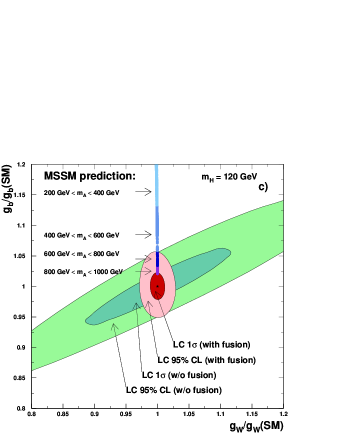
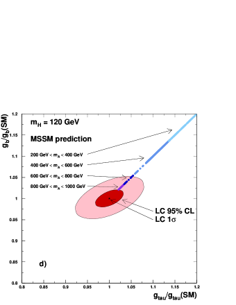
Figure 42: Higgs couplings determination at a LC (TESLA in this case) with 500 fb^-1 of data, for $M_{H}\!=\!120$ GeV. The labels with fusion and w/o fusion refers to $WW$-fusion inclusion/exclusion. From Ref. Aguilar-Saavedra:2001rg .

A LC will then be the ideal machine to discover small new physics effects. For instance, it could play a fundamental role in distinguishing the $h^{0}$ Higgs boson of the MSSM from the SM Higgs boson, in regions of the MSSM parameter space close to the decoupling limit. With this respect, Fig. 42 shows two combined fits: the first one combines the ratio between the bottom-quark Yukawa coupling to $h^{0}$ and its SM expected value and the ratio between the $h^{0}$ coupling to $W$ bosons and its SM expected value; the second one combines the same ratios for the bottom-quark and $\tau$-lepton Yukawa couplings. Different contours illustrates the precision with which the correlation between the combined ratios of couplings can be measured. On the same plots we see what the ratios would look like in the MSSM for different ranges of $M_{A}$. A definite distinction between SM and MSSM Higgs bosons can clearly be established.

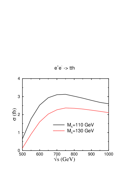
Figure 43: Cross section for $e^{+}e^{-}\rightarrow t\bar{t}H$, in the SM, as a function of the center of mass energy $\sqrt{s}$, for two different values of the Higgs boson mass.

The only problem in completing a full study of the Higgs boson couplings is the determination of the top-quark Yukawa coupling, and of the Higgs self couplings. The top-quark Yukawa coupling is indirectly determined by measuring the $t\bar{t}H$ cross section, when the $Z$ contribution is under control. This cross section is very small at $\sqrt{s}\!=\!500$ GeV, and peaks around $\sqrt{s}\!=\!800$ GeV (see Fig. 43) Recent studies show that with a LC operating at $\sqrt{s}\!=\!500$ GeV the top-quark Yukawa coupling, $y_{t}$, for a $M_{H}\!=\!120$ GeV Higgs boson, will probably be determined only at the 25% precision level, while with a LC operating at $\sqrt{s}\!=\!800$ GeV precisions as high as $5-6\%$ becomes available. An updated summary of the existing studies can be seen in Fig. 44. The initial phase of a high energy LC will therefore not be able to give us probably the most important Yukawa coupling, and with this respect the role of the LHC becomes crucial, since, as we have seen in Section III.4.2, the LHC can obtain $y_{t}$ within 10-15% accuracy, although with some intrinsic model dependence.

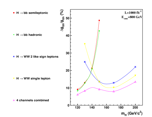
Figure 44: Expected accuracies for the measurement of the top-quark Yukawa coupling, $y_{t}$, in the process $e^{+}e^{-}\rightarrow t\bar{t}H$, as a function of $M_{H}$, for $\sqrt{s}\!=\!800$ GeV and 1 ab^-1 of data in various decay channels. From Ref. Djouadi:2005gi .

The production of Higgs boson pairs is also very rare (see Fig. 45), and the measurement of the Higgs boson self-couplings will probably have to wait for a very high energy Linear Collider, like the CLIC collider, a multi-TeV $e^{+}e^{-}$ machine being studied at CERN.

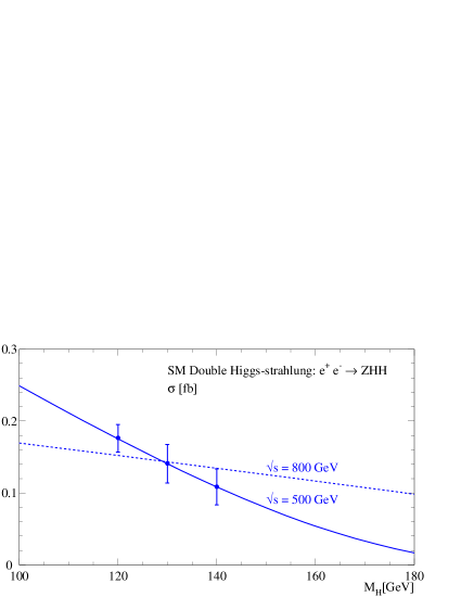
Figure 45: Cross section for $e^{+}e^{-}\rightarrow HHZ$, in the SM, as a function of $M_{H}$, for two values of the center of mass energy $\sqrt{s}$. The dots with error bars show the achievable experimental accuracies for 1000 fb^-1 of data. From Ref. Aguilar-Saavedra:2001rg .

Finally, the total width of a SM-like Higgs boson can be determined in a model independent way by using any well measured branching ratio. For example, one can use that $\Gamma\!=\!\Gamma(H\rightarrow WW^{*})/Br(H\rightarrow WW^{*})$, where $Br(H\rightarrow WW^{*})$ is measured directly and $\Gamma(H\rightarrow WW^{*})$ can be calculated from the direct determination of the $HWW$ coupling.

IV Highlights of theoretical calculations in Higgs boson physics

I would like to conclude these lectures by reviewing some important theoretical results that have recently been obtained in the calculation of Higgs boson physics observables, i.e. total and differential cross sections. Having to limit my discussion to a selection of topics, I prefer to focus on hadron colliders, since the discovery of a Higgs particle very much depends on our ability to provide precise theoretical predictions for hadronic cross sections. In this context I will concentrate on a few processes for which some outstanding progress has been made recently.

The cross section for $p\bar{p}$ and $pp$ collisions to produce a final state containing a Higgs bosons ($H$) can be schematically written as:

$$\sigma(pp,p\bar{p}\rightarrow H+X)=\sum_{ij}\int dx_{1}dx_{2}f_{i}^{p}(x_{1})f_{j}^{p,\bar{p}}(x_{2})\hat{\sigma}(ij\rightarrow H+X)\,\,\,,$$ (121)

where the partonic cross section $\hat{\sigma}(ij\rightarrow H+X)$ is convoluted with the Parton Distribution Functions (PDF) of partons $i$ and $j$. $f_{i}^{p,\bar{p}}(x)$ denotes indeed the PDF of parton $i$ into a proton (or anti-proton) and can be interpreted as the probability of finding parton $i$ into a proton (or anti-proton) with a fraction $x$ of its longitudinal momentum. Both the partonic cross section and the parton distribution functions are calculated perturbatively. At hadron colliders, the most important effects arise from strong interactions, and it is therefore mandatory to have the QCD perturbative expansion of $\sigma(pp,p\bar{p}\rightarrow H+X)$ under control. At each order in the perturbative expansion, the calculation of both $\hat{\sigma}(ij\rightarrow H+X)$ and $f_{i}^{p,\bar{p}}(x)$ contains ultraviolet divergences that are subtracted through a standard renormalization procedure. This, at each finite order, leaves a dependence on the renormalization scale, $\mu_{R}$. In the same way, when the PDF’s are defined, a factorization scale $\mu_{F}$ is introduced in the calculation of $f_{i}^{p,\bar{p}}(x)$. The dependence on both $\mu_{R}$ and $\mu_{F}$ is indicative of the residual theoretical uncertainty present at a given perturbative order, and should improve the higher the order of QCD corrections that are taken into account.

Indeed, it is well known that the theoretical predictions for most Higgs production hadronic cross sections at lowest or leading order (LO) are affected by a very large renormalization and factorization scale dependence. In general, at least the next-to-leading order (NLO) of corrections need to be calculated and this should stabilize or improve the theoretical prediction for the cross section, making the residual theoretical uncertainty comparable or smaller than the corresponding experimental precision. In some cases, as we will see, even next-to-next-to-leading order (NNLO) QCD corrections are necessary to obtain reliable theoretical predictions.

To be more specific, the NLO cross section for $pp,p\bar{p}\rightarrow H+X$ can in full generality be written as:

$$\sigma_{p\bar{p},pp}^{NLO}=\sum_{i,j}\int dx_{1}dx_{2}\mathcal{F}_{i}^{p}(x_{1},\mu_{R}\mu_{F}\mathcal{F}_{j}^{\bar{p},p}(x_{2},\mu_{R}\mu_{F}\hat{\sigma}_{ij}^{NLO}(x_{1},x_{2},\mu_{R},\mu_{F})\,\,\,,$$ (122)

where we have made explicit the dependence on both renormalization and factorization scale. $\mathcal{F}_{i}^{p,\bar{p}}$ denote the NLO PDF’s, while $\hat{\sigma}_{ij}^{NLO}$ is the parton level cross section calculated at NLO as:

$$\hat{\sigma}_{ij}^{NLO}=\hat{\sigma}_{ij}^{LO}+\frac{\alpha_{s}}{4\pi}\delta\hat{\sigma}_{ij}^{NLO}\,\,\,,$$ (123)

where $\delta\hat{\sigma}_{ij}$ represents the $\mathcal{O}(\alpha_{s})$ real and virtual corrections:

$$\delta\hat{\sigma}^{NLO}_{ij}=\hat{\sigma}^{ij}_{virt}+\hat{\sigma}^{ij}_{real}\,\,\,.$$ (124)

In a similar way, and with due differences, we could write $\sigma_{p\bar{p},pp}^{NNLO}$. A lot of theoretical effort has gone in recent years in the calculation of $\delta\hat{\sigma}^{NLO}_{ij}$ and $\delta\hat{\sigma}^{NNLO}_{ij}$ for several Higgs production processes. I have collected in Table 1 all the existing work on higher order QCD corrections to Higgs production modes. My apologies for any omission!

Table 1: Existing QCD corrections for various SM Higgs production processes.

process	$\sigma_{NLO,NNLO}$ by
$gg\rightarrow H$	S.Dawson, NPB 359 (1991), A.Djouadi, M.Spira, P.Zerwas, PLB 264 (1991) C.J.Glosser et al., JHEP 0212 (2002); V.Ravindran et al., NPB 634 (2002) D. de Florian et al., PRL 82 (1999) R.Harlander, W.Kilgore, PRL 88 (2002) (NNLO) C.Anastasiou, K.Melnikov, NPB 646 (2002) (NNLO) V.Ravindran et al., NPB 665 (2003) (NNLO) S.Catani et al. JHEP 0307 (2003) (NNLL), G.Bozzi et al., PLB 564 (2003),hep-ph/0508068
$q\bar{q}\rightarrow(W,Z)H$	T.Han, S.Willenbrock, PLB 273 (1991) O.Brien, A.Djouadi, R.Harlander, PLB 579 (2004) (NNLO)
$q\bar{q}\rightarrow q\bar{q}H$	T.Han, G.Valencia, S.Willenbrock, PRL 69 (1992) T.Figy, C.Oleari, D.Zeppenfeld, PRD 68 (2003)
$q\bar{q},gg\rightarrow t\bar{t}H$	W.Beenakker et al., PRL 87 (2001), NPB 653 (2003) S.Dawson et al., PRL 87 (2001), PRD 65 (2002), PRD 67,68 (2003)
$q\bar{q},gg\rightarrow b\bar{b}H$	S.Dittmaier, M.Krämer, M.Spira, PRD 70 (2004) S.Dawson et al., PRD 69 (2004), PRL 94 (2005)
$gb(\bar{b})\rightarrow b(\bar{b})H$	J.Campbell et al., PRD 67 (2003)
$b\bar{b}\rightarrow H$	D.A.Dicus et al. PRD 59 (1999); C.Balasz et al., PRD 60 (1999). R.Harlander, W.Kilgore, PRD 68 (2003) (NNLO)

The result of this effort can be naively summarized by investigating the residual renormalization ($\mu_{R}$) and factorization ($\mu_{F}$) scale dependence in each SM Higgs boson production mode. This is illustrated in Fig. 46 for the case of the LHC. For each production mode the scale $\mu\!=\!\mu_{R}\!=\!=\!\mu_{F}$ has been varied according to the corresponding original literature as indicated in Fig. 46, such that the scale interval can be different case by case. Since different production modes have very different cross sections, we have separated them into two plots, containing the leading and sub-leading production modes respectively.

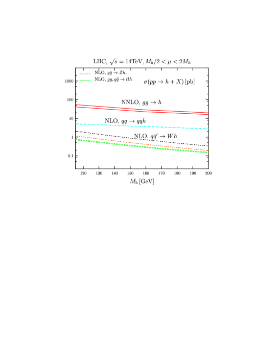
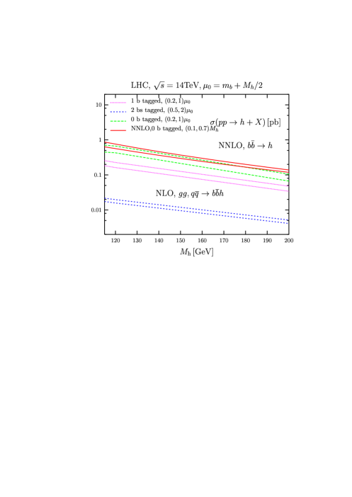
Figure 46: Residual renormalization and factorization scale dependence ($\mu\!=\!\mu_{R}\!=\!=\!\mu_{F}$) of the SM Higgs boson production cross section, when all available orders of QCD corrections are included. The scale $\mu$ is varied according to the original work present in the literature, and can therefore be slightly different case by case.

The bands in Fig. 46 are in no way indicative of the overall theoretical error, since they do not include systematic errors coming from PDFs and other input parameters. Moreover the effect of setting $\mu_{R}\neq\mu_{F}$ needs and has been investigated case by case, but it is not included in Fig. 46. Nevertheless Fig. 46 gives us a qualitative idea of the perturbative stability of the existing theoretical predictions for the SM Higgs boson production cross sections. Overall the existing theoretical predictions are in good control.

In a parallel series of lectures given at this school wacheroth:tasi04 you have been exposed to the complexity of higher order QCD calculations, and to the variety of techniques that have been developed to perform them. I will not then directly proceed and comment about the results of some higher order calculations in Higgs physics. In particular, I would like to report about: i) the calculation of $gg\rightarrow H$ at NNLO of QCD, a pioneer effort that has provided for the first time a reliable theoretical results for the most important Higgs production mode at hadron colliders; ii) the calculation of $pp,p\bar{p}\rightarrow t\bar{t}H,b\bar{b}H$ at NLO of QCD, a challenging task, due to the many massive degrees of freedom involved, that has provided for the first time reliable theoretical predictions for the cross sections of these two physically very important production modes. Both i) and ii) rely on the development of several innovative techniques that have allowed the successful completion of both calculations. Given the degree of technicalities involved, I will not review them in detail, but only point to the kind of difficulties that had to be faced. The interested reader can find all necessary technical details in the original literature, listed in Table  1 and in the bibliography.

IV.1 $gg\rightarrow H$ at NNLO

Figure 47: The $gg\rightarrow H$ production process at lowest order.

Most of the basic ideas that motivate the techniques used in the NNLO calculation of the cross section for the $gg\rightarrow H$ production process have been already introduced in Section III.1.4, where we discussed the $H\rightarrow gg$ loop-induced decay. In particular we know that in the SM, the main contribution to $gg\rightarrow H$ comes form the top-quark loop (see Fig. 47) since:

$$\sigma_{LO}=\frac{G_{F}\alpha_{s}(\mu)^{2}}{288\sqrt{2}\pi}\left|\sum_{q}A_{q}^{H}(\tau_{q})\right|^{2}\,\,\,,$$ (125)

where $\tau_{q}=4m_{q}^{2}/M_{H}^{2}$ and $A_{q}^{H}(\tau_{q})\leq 1$ with $A_{q}^{H}(\tau_{q})\rightarrow 1$ for $\tau_{q}\rightarrow\infty$.

$\longrightarrow$

Figure 48: The top-quark loop contribution to $gg\rightarrow H$ gives origin to a $ggH$ effective vertex in the $m_{t}\rightarrow\infty$ limit.

As we saw in Section III.1.4, one can work in the infinite top-quark mass limit and reduce the one-loop $Hgg$ vertex to a tree level effective vertex, derived from an effective Lagrangian of the form:

$$\mathcal{L}_{eff}=\frac{H}{4v}C(\alpha_{s})G^{a\mu\nu}G^{a}_{\mu\nu}\,\,\,,$$ (126)

where the coefficient $C(\alpha_{s})$, including NLO and NNLO QCD corrections, can be written as:

$$C(\alpha_{s})=\frac{1}{3}\frac{\alpha_{s}}{\pi}\left[1+c_{1}\frac{\alpha_{s}}{\pi}+c_{2}\left(\frac{\alpha_{s}}{\pi}\right)^{2}+\cdots\right]\,\,\,.$$ (127)

NLO and NNLO QCD corrections to $gg\rightarrow H$ can then be calculated as corrections to the effective $Hgg$ vertex, and the complexity of the calculation is reduced by one order of loops.

The NLO order of QCD corrections has actually been calculated both with and without taking the infinite top-quark mass limit. The comparison between the exact and approximate calculation shows an impressive agreement at the level of the total cross section, and, in particular, at the level of the $K$-factor, i.e. the ratio between NLO and LO total cross sections ($K\!=\!\sigma_{NLO}/\sigma_{LO}$), as illustrated in Fig. 49.

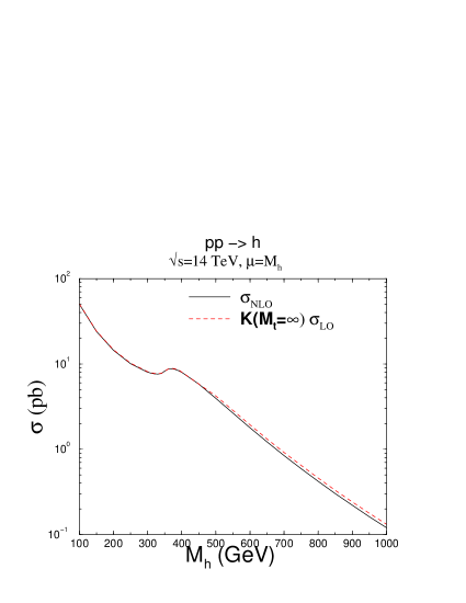
Figure 49: The NLO cross section for $gg\rightarrow H$ as a function of $M_{H}$. The two curves represent the results of the exact calculation (solid) and of the infinite top-quark mass limit calculation (dashed), where the NLO cross section has been obtained as the product of the $K$-factor ($K\!=\!\sigma_{NLO}/\sigma_{LO}$) calculated in the $m_{t}\!\rightarrow\!\infty$ limit times the LO cross section. From Ref. Dawson:1998yi .

It is indeed expected that methods like the infinite top quark mass limit may not reproduce the correct kinematic distributions of a given process at higher order in QCD, but are very reliable at the level of the total cross section, in particular when the cross section receives large momentum independent contribution at the first order of QCD corrections. As for the $H\rightarrow gg$ decay process, the NLO corrections to $gg\rightarrow H$ are very large, changing the LO cross section by more than 50%. Since the $gg\rightarrow H$ is the leading Higgs boson production mode at hadron colliders, it has been clear for quite a while that a NNLO calculation was needed in order to understand the behavior of the perturbatively calculated cross section, and if possible, in order to stabilize its theoretical prediction.

Recently the NNLO corrections to the total cross section have been calculated using the infinite top-quark mass limit (see Table 1). The calculation of the NNLO QCD corrections involves then 2-loop diagrams like the ones shown in Fig. 50, instead of the original 3-loop diagrams (a quite formidable task!).

Figure 50: Two-loop diagrams that enter the NNLO QCD corrections to $gg\rightarrow H$.

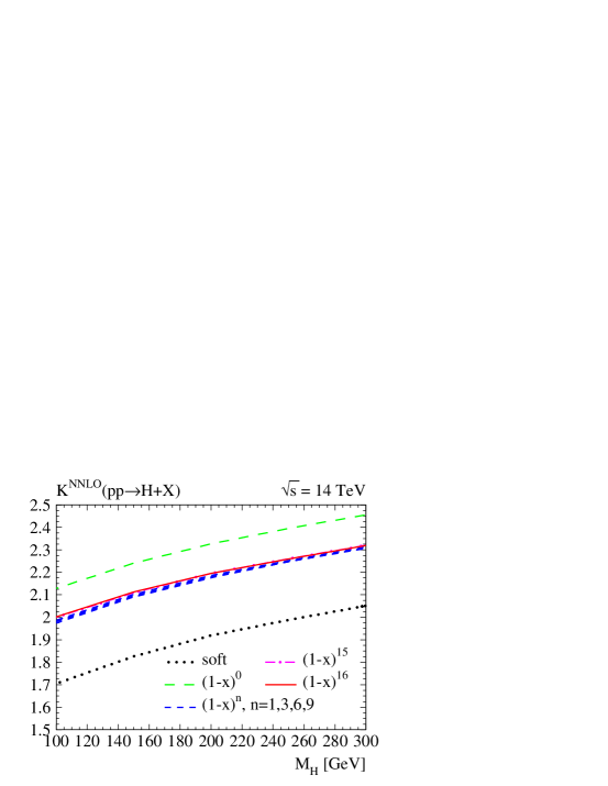
Figure 51: $K$-factor for $gg\rightarrow H$ at the LHC ($\sqrt{s}\!=\!14$ TeV), calculated adding progressively more terms in the expansion of Eq. (129). From Harlander and Kilgore as given in Table 1.

Moreover, thanks to the $2\rightarrow 1$ kinematic of the $gg\rightarrow H$ process, the cross section has in one case be calculate in the so called soft limit, i.e. as an expansion in the parameter $x\!=\!M_{H}^{2}/\hat{s}$ about $x\!=\!1$, where $\hat{s}$ is the partonic center of mass energy (see paper by Harlander and Kilgore in Table 1). The $n$-th term in the expansion of $\hat{\sigma}_{ij}$ of Eq. (121):

$$\hat{\sigma}_{ij}=\sum_{n\geq 0}\left(\frac{\alpha_{s}}{\pi}\right)^{n}\hat{\sigma}^{(n)}_{ij}\,\,\,,$$ (128)

can then be written in the soft limit ($x\rightarrow 1$) as follows:

$$\hat{\sigma}^{(n)}_{ij}=\underbrace{a^{(n)}\delta(1-x)+\sum_{k=0}^{2n-1}b_{k}^{(n)}\left[\frac{\ln^{k}(1-x)}{1-x}\right]_{+}}_{\mbox{purely soft terms}}+\underbrace{\sum_{l=0}^{\infty}\sum_{k=0}^{2n-1}c_{lk}^{(n)}(1-x)^{l}\ln^{k}(1-x)}_{\mbox{collinear+hard terms}}$$ (129)

where we have made explicit the origin of different terms in the expansion. The NNLO cross section is then obtained by calculating the coefficients $a^{(2)}$, $b^{(2)}_{k}$ , and $c^{(2)}_{lk}$, for $l\geq 0$ and $k\!=\!0,\ldots,3$.

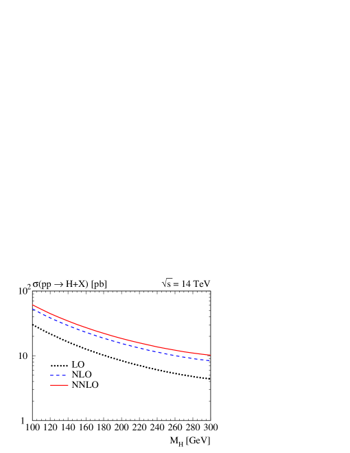
Figure 52: Cross section for $gg\rightarrow H$ at the LHC ($\sqrt{s}\!=\!14$ TeV), calculated at LO, NLO and NNLO of QCD corrections, as a function of $M_{H}$, for $\mu_{F}\!=\!\mu_{R}\!=\!M_{H}/4$. From Harlander and Kilgore in Table 1.

In Fig. 51 we see the convergence behavior of the expansion in Eq. (129). Just adding the first few terms provides a remarkably stable $K$-factor. The results shown in Fig. 51 have been indeed confirmed by a full calculation Anastasiou:2002yz , where no soft approximation has been used.

The results of the NNLO calculation Harlander:2002wh ; Anastasiou:2002yz are illustrated in Figs. 52 and 53.

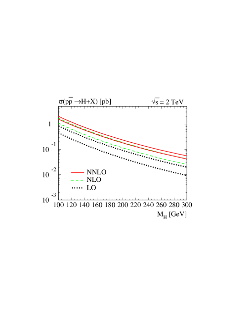
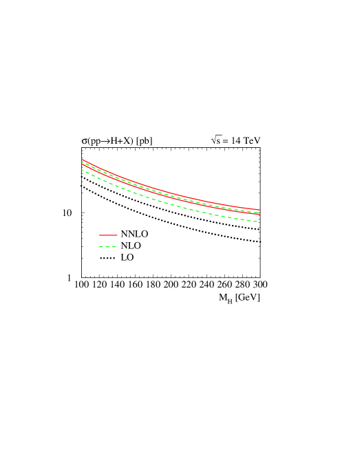
Figure 53: Residual renormalization/factorization scale dependence of the LO, NLO, and NNLO cross section for $gg\rightarrow H$, at the Tevatron ($\sqrt{s}\!=\!2$ TeV) and at the LHC ($\sqrt{s}\!=\!14$ TeV), as a function of $M_{H}$. The bands are obtained by varying $\mu_{R}\!=\!\mu_{F}$ by a factor of 2 about the central value $\mu_{F}\!=\!\mu_{R}\!=\!M_{H}/4$. From Ref. Harlander:2002wh .

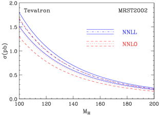
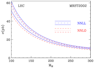
Figure 54: NNLL and NNLO cross sections for Higgs boson production via gluon-gluon fusion at both the Tevatron and the LHC. From Ref. Catani:2003zt

In Fig. 52 we can observe the convergence of the perturbative calculation of $\sigma(gg\rightarrow H$), since the difference between NLO and NNLO is much smaller than the original difference between LO and NLO. This is further confirmed in Fig. 53, where we see that the uncertainty band of the NNLO cross section overlaps with the corresponding NLO band. Therefore the NNLO term in the perturbative expansion only modify the NLO cross section within its NLO theoretical uncertainty. This is precisely what one would expect from a good convergence behavior. Moreover, the narrower NNLO bands in Fig. 53 shows that the NNLO result is pretty stable with respect to the variation of both renormalization and factorization scales. This has actually been checked thoroughly in the original papers, by varying both $\mu_{R}$ and $\mu_{F}$ independently over a range broader than the one used in Fig. 53.

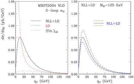
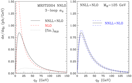
Figure 55: The $q_{T}$ spectrum at the LHC with $M_{H}\!=\!125$ GeV. The upper plots show: (left) setting $\mu_{R}\!=\!\mu_{F}\!=\!Q\!=\!M_{H}$, the results at NNL+LO accuracy compared with the LO spectrum and the finite component of the LO spectrum; (right) the uncertainty band from the variation of the scales $\mu_{R}$ and $\mu_{F}$ at NLL+LO accuracy. The lower plots show the same at NNLL+NLO accuracy. From Ref. Bozzi:2005wk .

The NNLO cross section for $gg\rightarrow H$ has been further improved by Catani et al. Catani:2003zt by resumming up to the next-to-next-to leading order of soft logarithms. Using the techniques explained in their papers, they have been able to obtain the theoretical results shown in Figs. 54 and 55 for the total and differential cross sections respectively. In particular, we see from Fig. 54 that the NNLO and NNLL results nicely overlap within their uncertainty bands, obtained from the residual renormalization and factorization scale dependence. The residual theoretical uncertainty of the NNLO+NNLL results has been estimated to be 10% from perturbative origin plus 10% from the use of NLO PDF’s instead of NNLO PDF’s. Moreover, in Fig. 55 we see how the resummation of NNL crucially modify the shape of the Higgs boson transverse momentum distribution at low transverse momentum ($q_{T}$), where the soft $\ln(M_{H}^{2}/q_{T}^{2})$ are large and change the behavior of the perturbative expansion in $\alpha_{s}$ Bozzi:2005wk .

IV.2 $pp,p\bar{p}\rightarrow t\bar{t}H$ and $pp,p\bar{p}\rightarrow b\bar{b}H$ at NLO

The associated production of a Higgs boson with heavy quark pairs, $pp,p\bar{p}\rightarrow t\bar{t}H$ and $b\bar{b}H$, has been for a while the only Higgs production process for which the NLO of QCD corrections had not been calculated. Given the relevance of both production modes to Higgs physics (see discussion in Section III.4) and the large renormalization and factorization scale dependence of the LO cross sections (see, e.g., the LO curves in Figs. 59 and 62), a full NLO calculation was mandatory. This has been completed in the papers by Beenakker et al. Beenakker:2001rj ; Beenakker:2002nc and Dawson et al. Reina:2001sf ; Reina:2001bc ; Dawson:2002tg ; Dawson:2003zu listed in Table 1 and we will briefly report about their most important results in this Section.

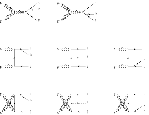
Figure 56: Tree level Feynman diagrams for $q\bar{q}\rightarrow t\bar{t}H$ and $gg\rightarrow t\bar{t}H$. Analogous diagrams, with $t\rightarrow b$, contribute to the $q\bar{q}\rightarrow b\bar{b}H$ and $gg\rightarrow b\bar{b}H$ processes.

The NLO calculation of $pp,p\bar{p}\rightarrow Q\bar{Q}H$ (for $Q\!=\!b,t$) presents several challenges, since it has to deal with a $2\rightarrow 3$ process that involves all massive particles in the final state. At tree level, $Q\bar{Q}H$ proceeds through the $q\bar{q},gg\rightarrow Q\bar{Q}H$ parton level processes illustrated in Fig. 56 for $Q\!=\!t$. As expected, the $q\bar{q}\rightarrow Q\bar{Q}H$ dominates for large fraction of the parton longitudinal momentum $x$, while $gg\rightarrow Q\bar{Q}H$ dominates at small $x$. This translate into the fact that the parton level cross section for $t\bar{t}H$ production is dominated by $q\bar{q}\rightarrow t\bar{t}H$ at the Tevatron, and by $gg\rightarrow t\bar{t}H$ at the LHC, while $b\bar{b}H$ production is always dominated by $gg\rightarrow b\bar{b}H$. The $\mathcal{O}(\alpha_{s})$ virtual corrections include up to pentagon diagrams, such that the problem of calculating scalar and tensor integrals with up to five denominators, several of which massive, has to be faced. Most integrals have to be calculated analytically since both ultraviolet (UV) and infrared (IR) singularities have to be extracted. The $\mathcal{O}(\alpha_{s})$ real corrections involve factoring out IR (soft and collinear) divergences from a $2\rightarrow 4$ phase space with several massive particles. Samples of Feynman diagrams corresponding to the $\mathcal{O}(\alpha_{s})$ virtual and real corrections are illustrated in Figs. 57 and 58.

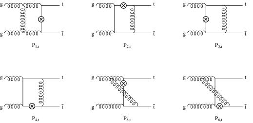
Figure 57: Example of $\mathcal{O}(\alpha_{s})$ virtual corrections to $gg\rightarrow t\bar{t}H$: pentagon diagrams. The circled crosses denote all possible insertion of the final Higgs boson leg. All $t$-channel diagrams have corresponding $u$ channel diagrams, where the two initial state gluon legs are crossed. Analogous diagrams with $t\rightarrow b$ contribute to the $\mathcal{O}(\alpha_{s})$ virtual corrections to $gg\rightarrow b\bar{b}H$.

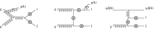
Figure 58: Examples of $\mathcal{O}(\alpha_{s})$ real corrections to $gg\rightarrow t\bar{t}H$. The circled crosses denote all possible insertion of the final Higgs boson leg. Analogous diagrams with $t\rightarrow b$ contribute to the $\mathcal{O}(\alpha_{s})$ real corrections to $gg\rightarrow b\bar{b}H$.

Several new methods and algorithms have been used by the two collaborations that have calculated the NLO cross section for $pp,p\bar{p}\rightarrow Q\bar{Q}H$, and we refer to their papers for all technical details. In the following we will comment separately on $t\bar{t}H$ and $b\bar{b}H$ NLO results.

For $t\bar{t}H$ production, the most important outcome of the full NLO calculation is illustrated in Fig. 59, where the renormalization ($\mu_{R}$) and factorization scale ($\mu_{F}$) dependence of the LO and NLO total inclusive cross section is presented, for a SM Higgs boson mass of $M_{H}\!=\!120$ GeV, at both the Tevatron and the LHC. We note that the factorization and renormalization scales have been set equal in the plots of Fig. 59, $\mu_{R}=\mu_{F}=\mu$, while in the original work both scales have been first varied independently to verify that $\mu_{R}=\mu_{F}=\mu$ is not a particular point at which both scale dependences accidentally mutually cancel. It is evident from the plots of Fig. 59 that the NLO total cross section sensitivity to $\mu_{R}$ and $\mu_{F}$ is drastically reduced with respect to the LO cross section. Indeed, the residual systematic error coming from scale dependence is at NLO reduced to about 15%, as opposed to more than 100% of the LO cross section. The NLO predictions for $t\bar{t}H$ production can now be confidently used to interface with experimental analyses.

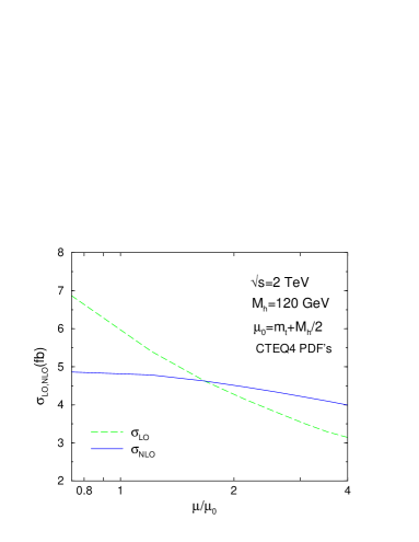
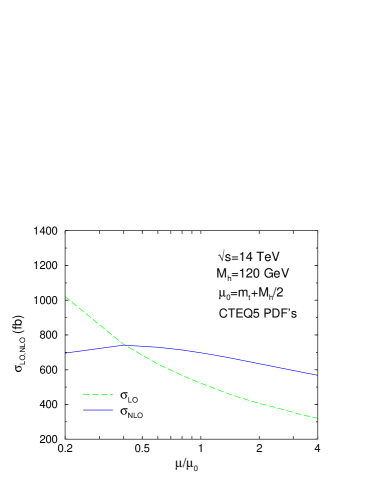
Figure 59: Dependence of $\sigma_{LO,NLO}(p\bar{p},pp\rightarrow t\bar{t}H)$ on the renormalization/factorization scale $\mu$, at both the Tevatron and the LHC, for $M_{H}\!=\!120$ GeV. The reference scale $\mu_{0}$ is taken to be $\mu_{0}\!=\!m_{t}+M_{H}/2$. From Refs. Reina:2001bc and Dawson:2003zu .

Let us now consider $b\bar{b}H$ production. Naively, one would expect the calculation of $b\bar{b}H$ production at NLO to follow that of $t\bar{t}H$, with the universal replacement of the top-quark mass with the bottom-quark mass, $m_{t}\leftrightarrow m_{b}$. However, the theoretical prediction of $b\bar{b}H$ production at hadron colliders involves a few subtle issues not encountered in the calculation of $t\bar{t}H$ production. Indeed, both from the experimental and theoretical standpoint, it is important to distinguish between inclusive and exclusive $b\bar{b}H$ production. More specifically, the production of a Higgs boson with a pair of $b$ quarks can be detected via: (i) a fully exclusive measurement, where both $b$ jets are observed, (ii) a fully inclusive measurement, where no $b$ jet is observed, or (iii) a semi-inclusive measurement, where at least one $b$ jet is observed.

Experimentally, $b$ quarks are identified or tagged by imposing selection cuts on their transverse momentum and their angular direction with respect to the beam axis or pseudorapidity. Inclusive modes have larger cross sections, but also larger background, such that more exclusive modes are often preferred experimentally. Moreover, only the exclusive and semi-inclusive modes are unambiguously proportional to the bottom-quark Yukawa coupling.

Theoretically, different approaches may be adopted depending on the fact that a final state $b$ quark is either treated inclusively (untagged) or exclusively (tagged). Indeed, when a final state $b$ quark is not identified through some selection cuts, the corresponding integration over its phase space, in particular over its transverse momentum, gives rise to logarithms of the form:

$$\Lambda_{b}=\log\biggl{(}\frac{\mu_{H}^{2}}{m_{b}^{2}}\biggr{)}\,\,,$$ (130)

where $m_{b}$ and $\mu_{H}$ represent the lower and upper bounds of the integration over the transverse momentum of the final state $b$ quark. $\mu_{H}$ is typically of $\mathcal{O}(M_{H})$ and therefore, due to the smallness of the bottom-quark mass, these logarithms can be quite large. Additionally, the same logarithms appear at every order in the perturbative expansion of the cross section in $\alpha_{s}$, due to recursive gluon emission from internal bottom-quark lines. If the logarithms are large, the convergence of the perturbative expansion of the cross section could be severely hindered and it can be advisable to reorganize the expansion in powers of $\alpha_{s}^{n}\Lambda_{b}^{m}$, further resumming various orders of logarithms via renormalization group techniques.

Currently, there are two approaches to calculating the inclusive and semi-inclusive cross sections for Higgs production with bottom quarks. Working under certain kinematic approximations, and adopting the so-called five-flavor-number scheme (5FNS), the collinear logarithms, $\Lambda_{b}$, can be factored out and resummed by introducing a bottom-quark Parton Distribution Function (PDF) Barnett:1987jw ; Olness:1987ep ; Dicus:1988cx . This approach restructures the calculation to be an expansion in both $\alpha_{s}$ and $\Lambda_{b}^{-1}$. At tree level, the semi-inclusive production is then described by the process $bg\rightarrow bH$ illustrated in Fig. 60, while the fully inclusive production process becomes $b\bar{b}\rightarrow H$, illustrated in Fig. 61. Alternatively, working with no kinematic approximations, and adopting the so-called four-flavor-number scheme (4FNS), one can compute the cross section for $p\bar{p},pp\to b\bar{b}H$ at fixed order in QCD with no special treatment of the collinear logarithms, considering just the parton level processes $q\bar{q},gg\to b\bar{b}H$ illustrated in Fig. 56 (with $t\rightarrow b$) and their radiative corrections.

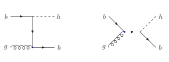
Figure 60: Tree level Feynman diagram for $bg\to bH$ in the 5FNS.

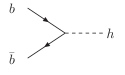
Figure 61: Tree level Feynman diagram for $b\bar{b}\to H$ in the 5FNS.

The fully exclusive $b\bar{b}H$ production cross section can only be computed in the 4FNS framework. As far as the inclusive and semi-inclusive production cross sections go, the comparison between the 4FNS and 5FNS needs to consider QCD corrections beyond the LO, in order to work with stable results. Indeed, the two calculation schemes represent different perturbative expansion of the same physical cross section, and therefore should agree at sufficiently high order. The discussion to follow is based on the NLO calculation of $q\bar{q},gg\to b\bar{b}H$ Dittmaier:2003ej ; Dawson:2003kb and $bg\rightarrow bH$ Campbell:2002zm , and on the NNLO calculation of $b\bar{b}\rightarrow H$ Harlander:2003ai .

It should be noted that our discussion for the production of a scalar Higgs boson with bottom quarks applies equally well to the production of a pseudoscalar Higgs boson. In fact, if one neglects the bottom-quark mass in the calculation of the NLO corrections, the predictions for $b\bar{b}A^{0}$ is identical to those for $b\bar{b}h^{0}(H^{0})$ upon rescaling of the Yukawa couplings (see Section II.4.4). On the other hand, for massive $b$ quarks, the situation becomes more complicated due to the $\gamma_{5}$ matrix appearing in the $b\bar{b}A^{0}$ Yukawa coupling. The $\gamma_{5}$ Dirac matrix is intrinsically a four-dimensional object and care must be taken in its treatment when regularizing the calculation in dimensional regularization ($d\neq 4$). However, bottom-quark mass effects are expected to be small, $\mathcal{O}(\frac{m_{b}^{2}}{M_{h}^{2}})$, and predictions for $b\bar{b}h^{0}$, upon rescaling of the Yukawa coupling, provide good estimates of $b\bar{b}A^{0}$ production even in the massive $b$-quark case. In the following we will present results for the exclusive, semi-inclusive, and inclusive cross sections separately.

The fully exclusive $b\bar{b}H$ NLO total cross section is illustrated in Figs. 62 and 63, both for the Tevatron and for the LHC. Both $b$ quarks in the final state are identified by the cuts explicitly given in Fig. 62, which have been chosen to closely mimic experimental searches. The curves in Fig. 62 show the dependence of the LO and NLO exclusive $b\bar{b}H$ cross section from both renormalization and factorization scales (set equal in these plots, i.e. $\mu_{R}\!=\!\mu_{F}\!=\!\mu$). The two sets of curves represent the case in which the bottom-quark mass in the bottom-quark Yukawa coupling is renormalized in the on-shell scheme ($OS$, blue curves) or in the modified Minimal Subtraction scheme ($\overline{MS}$, red curves). As we have already observed in Section III.1.3 when we considered the decays of a Higgs boson into quark pairs, the bottom-quark renormalized mass varies substantially when the renormalization scale $\mu$ is varied from scales of the order of $m_{b}$ to scales of the order of $M_{H}$, and therefore it is important to know how the large logarithms that determine the running of $m_{b}$ are treated in the different renormalization schemes. This is particularly true for the factor $m_{b}$ that appears in the bottom-quark Yukawa coupling, $y_{b}\!=\!m_{b}/v$, since the cross section depends quadratically on $y_{b}$. It is much less relevant for the cross section kinematic dependence on $m_{b}$, coming from the amplitude square or from the integration over the final state phase space. For this reason, the $OS$ and $\overline{MS}$ labels in Fig. 62 refer to the cases in which only the bottom-quark mass in $y_{b}$ is renormalized one way or the other. The kinematic $b$-quark mass is always taken to be the pole mass.

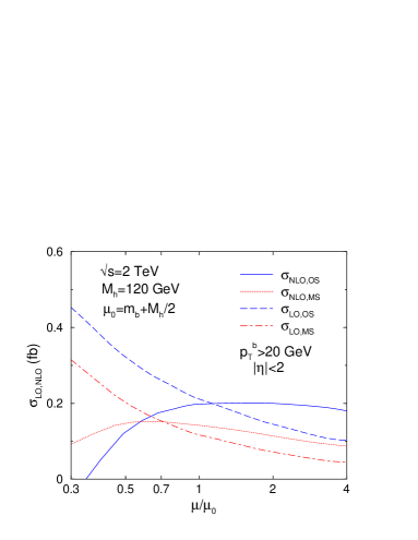
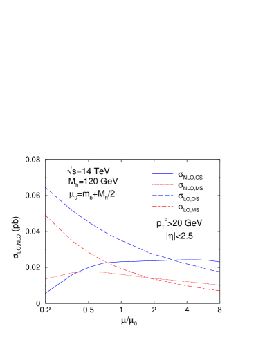
Figure 62: Scale dependence of the LO and NLO cross sections for $p\bar{p}\rightarrow b\bar{b}H$ (Tevatron) and $pp\rightarrow b\bar{b}H$ (LHC), for $M_{H}\!=\!120$ GeV. The curves labeled $\sigma_{LO,OS}$ and $\sigma_{NLO,OS}$ use the $OS$ renormalization scheme, while the curves labeled $\sigma_{LO,MS}$ and $\sigma_{NLO,MS}$ use the $\overline{MS}$ renormalization scheme. From Ref. Dawson:2003kb .

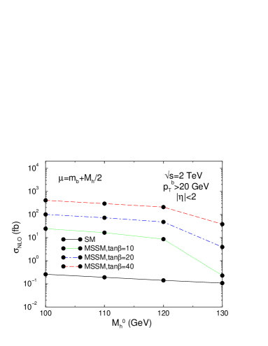
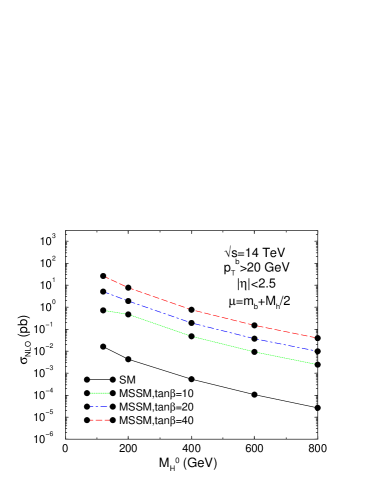
Figure 63: NLO cross section for $p\bar{p}\rightarrow b\bar{b}H$ (Tevatron) and $pp\rightarrow b\bar{b}H$ (LHC) as a function of $M_{H}$, in the SM and in the MSSM with $\tan\beta\!=\!10,20$ and $40$. For the Tevatron the production process considered is $p\bar{p}\to b\bar{b}h^{0}$ with $M_{h^{0}}\!=\!100,110,120$, and 130 GeV, while for the LHC it is $pp\to b\bar{b}H^{0}$ with $M_{H^{0}}\!=\!120,200,400,600$, and 800 GeV. From Ref. Dawson:2003kb .

Looking at the curves in Fig. 62 we learn that, as expected, the NLO set of QCD corrections stabilizes the total cross section, drastically reducing the scale dependence of the LO cross section. Moreover we see that there is a non negligible dependence on the bottom-quark mass renormalization scheme. This dependence is intrinsic of any perturbative calculation, and should decrease the more orders are added in the perturbative expansion of a given physical observable. However, from the behavior of the residual scale dependence, it is possible to estimate which renormalization scheme provides a better perturbative expansion. In the case illustrated in Fig. 62, both $OS$ and $\overline{MS}$ NLO cross sections show a well defined plateau region where the cross section is very mildly dependent on the scale $\mu$. Nevertheless, the $\overline{MS}$ cross section overall performs better, since it has a more regular behavior also at small scales. As a result, $\overline{MS}$ is often the preferred choice in all processes that depend on the bottom-quark Yukawa coupling. Finally, Fig. 63 shows the dependence of the total cross section from the Higgs boson mass, in both the SM (solid black curve) and the MSSM (dashed colored curves, corresponding to different values of $\tan\beta$), over a significant $M_{H}$ range for both the Tevatron and the LHC. The quadratic growth of the MSSM cross sections with $\tan\beta$ is evident, and this graphically confirms the possibility of finding evidence of new physics already at the Tevatron, if an MSSM-like 2HDM with large $\tan\beta$ is realized in nature (see Sec. III.4.3).

Let us now turn to the semi-inclusive and inclusive $b\bar{b}H$ cross sections. For both production modes, much effort has been spent recently in understanding the difference between 4FNS and 5FNS in order to assess the reliability of the existing theoretical resultsCampbell:2004pu ; Dittmaier:2003ej ; Kramer:2004ie ; Dawson:2004sh . First of all, let us briefly review the idea behind the introduction of a bottom-quark PDF, which naturally leads to the 5FNS framework. For the purpose of illustration, consider the prototype case depicted in Fig. 64: one of the final state bottom quarks is directly originating from the $g\rightarrow b\bar{b}$ splitting of one of the initial state gluons, while the shaded blob represents all the possible non collinear configurations of the remaining particles. In the $m_{b}\rightarrow 0$ limit, the $g\rightarrow b\bar{b}$ configuration gives origin to collinear singularities, when the two $b$ quarks are emitted in the same direction of the splitting gluon. In the case of $b\bar{b}H$ production, the singularities appear in the $p_{T}^{b}\rightarrow 0$ phase space region, where $p_{T}^{b}$ is the transverse momentum of the upper leg bottom quark in Fig. 64. If we take $m_{b}\neq 0$, these singularities are regulated by the non zero $b$-quark mass, leaving behind collinear logarithms $\Lambda_{b}$ of the form given in Eq. (130).

Figure 64: Tree level Feynman diagrams for $gg\rightarrow b\bar{b}H$ illustrating the almost collinear emission of a bottom quark (upper leg).

The contribution to the total partonic cross section from this diagram can be written as:

$$d\hat{\sigma}_{gg\rightarrow b\bar{b}H} = \frac{1}{(2)2E_{1}2E_{2}}\frac{d^{3}p_{b}}{(2\pi)^{3}}\frac{1}{2E_{b}}\frac{d^{3}p_{\bar{b}}}{(2\pi)^{3}}\frac{1}{2E_{\bar{b}}}\frac{d^{3}p_{H}}{(2\pi)^{3}}\frac{1}{2E_{H}}\overline{\sum}|\mathcal{M}_{gg\rightarrow b\bar{b}H}|^{2}$$

$$\cdot(2\pi)^{4}\delta^{(4)}(q_{1}+q_{2}-p_{b}-p_{\bar{b}}-p_{H})\,\,\,,$$ (131)

where we have used the momentum notation of Fig. 64, such that $E_{1,2}$ are the energies of the initial gluons while $E_{b,\bar{b},H}$ are the energies of the final state particles. The amplitude for this process is denoted by $\mathcal{M}_{gg\rightarrow b\bar{b}H}$. Parameterizing the $b$-quark propagator momentum as:

$$k^{\mu}=zq^{\mu}_{1}+\beta n^{\mu}+k^{\mu}_{\perp}\,\,\,,$$ (132)

where $z$ is the fraction of the initial gluon momentum carried by the $b$ quark, and $k^{\mu}_{\perp}$ is transverse to both $q^{\mu}_{1}$ and $n^{\mu}$, for an arbitrary vector $n^{\mu}$, with $k^{\mu}_{\perp}k_{\perp\mu}=-k_{T}^{2}$, one can explicitly show (after some Dirac algebra manipulations) that:

$$|\mathcal{M}_{gg\rightarrow b\bar{b}H}|^{2}\simeq g_{s}^{2}C_{F}\frac{4}{k_{T}^{2}}\left(\frac{1-z}{z}\right)P_{qg}(z)|\mathcal{M}_{g\bar{b}\rightarrow\bar{b}H}|^{2}\,\,\,,$$ (133)

where $P_{qg}(z)$ is the Altarelli-Parisi splitting function for $g\rightarrow q\bar{q}$:

$$P_{qg}=\frac{1}{2}[z^{2}+(1-z)^{2}]\,\,\,,$$ (134)

$C_{F}=(N^{2}-1)/2/N$ (for $N\!=\!3$ colors), and $\mathcal{M}_{g\bar{b}\rightarrow\bar{b}h}$ is the amplitude for $g\bar{b}\rightarrow\bar{b}H$. The previous equation is approximate, i.e. it has been obtained by neglecting higher powers of $k_{T}^{2}$, keeping only the terms that would give the most singular or leading contribution upon integration over the collinear $b$-quark phase space:

$$\frac{d^{3}p_{b}}{(2\pi)^{3}}\frac{1}{2E_{b}}\simeq\frac{1}{16\pi^{2}}\frac{dzdk_{T}^{2}}{(1-z)}\,\,\,,$$ (135)

where we have used that in the small $k_{T}$ limit the transverse part of the four momentum of the outgoing quark, $p_{b}^{T}$ coincides with $k_{T}$. Inserting Eqs. (133) and (135) into Eq. (IV.2) one finds:

$$d\hat{\sigma}_{gg\rightarrow b\bar{b}H}\simeq\frac{dk_{T}^{2}}{k_{T}^{2}}dz\frac{\alpha_{s}}{2\pi}P_{qg}(z)d\hat{\sigma}_{g\bar{b}\rightarrow\bar{b}H}\,\,\,.$$ (136)

The integration over $k_{T}^{2}$, with lower bound $m_{b}^{2}$ and upper bound $\mu_{H}^{2}$, gives origin to the collinear logarithm $\Lambda_{b}$ introduced in Eq. (130). Moreover, when one convolutes with the gluon PDFs, $g(x_{i},\mu)$ (for $i\!=\!1,2$), of the two initial gluons to obtain the hadronic cross section, a bottom-quark PDF of the form:

$$b(x,\mu_{F})=\frac{\alpha_{s}(\mu_{F})}{2\pi}\Lambda_{b}\int_{x}^{1}\frac{dy}{y}P_{qg}\left(\frac{x}{y}\right)g(y,\mu_{F})\,\,\,$$ (137)

naturally appears. In Eq. (137) $\mu_{F}$ represents the factorization scale. The collinear $\Lambda_{b}$ logarithms are factored out and then resummed in the bottom-quark PDF when the factorization scale is set to $\mu_{F}\!=\!\mu_{H}$. Indeed, Eq. (137) gives the bottom-quark parton density at the lowest order in $\alpha_{s}$, while the leading $\alpha_{s}^{n}\Lambda_{b}^{n}$ logarithms are resummed via the DGLAP equation upon evolution:

$$\frac{d}{d\log\mu}\,b(x,\mu)=\frac{\alpha_{s}(\mu)}{\pi}\int_{x}^{1}\frac{dy}{y}P_{qg}\left(\frac{x}{y}\right)\,g(y,\mu)\,\,\,.$$ (138)

The 5FNS approach is therefore based on the approximation that the outgoing $b$ quarks are at small transverse momentum, since this is the region of phase space that is emphasized by the $k_{T}$ expansion. The incoming $b$ partons are given zero momentum at leading order, and acquire transverse momentum at higher order. With the use of a $b$-quark PDF, the 5FNS effectively reorders the perturbative expansion to be one in $\alpha_{s}$ and $\Lambda_{b}^{-1}$. To see how this works, let us consider the perturbative expansion of the inclusive process $b\bar{b}\rightarrow H$ (Fig. 61) which, according to what we just saw, is intrinsically of order $\alpha_{s}^{2}\Lambda_{b}^{2}$. At NLO, the virtual and real corrections to the tree level process make contributions of $\mathcal{O}(\alpha_{s}^{3}\Lambda_{b}^{2})$. However, at NLO, we must also consider the contribution from $bg\rightarrow bH$ where the final state $b$ is at high transverse momentum. This process makes a contribution of order $\alpha_{s}^{2}\Lambda_{b}$ and is, thus, a correction of $\mathcal{O}(\Lambda_{b}^{-1})$ to the tree level cross section. Similarly, at NNLO, besides the myriad of radiative corrections of $\mathcal{O}(\alpha_{s}^{4}\Lambda_{b}^{2})$, we must also include the contribution from the process $gg\rightarrow b\bar{b}H$, where both $b$ and $\bar{b}$ are at high $p_{T}$. The contribution from these diagrams are of order $\alpha_{s}^{2}$, and are, thus, $\mathcal{O}(\Lambda_{b}^{-2})$ (or NNLO) corrections to the tree level process $b\bar{b}\rightarrow H$ Dicus:1988cx ; Dicus:1998hs . The above discussion for $b\bar{b}\to h$ also applies to the perturbative expansion of $bg\rightarrow bH$. In this case, the tree level process is of order $\alpha_{s}^{2}\Lambda_{b}$ and the contribution from $gg\rightarrow b\bar{b}H$ is a NLO correction of $\mathcal{O}(\Lambda_{b}^{-1})$  Campbell:2002zm .

The comparison between 4FNS and 5FNS has been initially performed in the SM Campbell:2004pu ; Dittmaier:2003ej ; Kramer:2004ie ; Dawson:2004sh . This has been crucial to understand several important issues. However, since the production of a Higgs boson with bottom quarks will only be physically interesting if the bottom-quark Yukawa coupling is enhanced beyond its SM value, we will present the 4FNS vs 5FNS comparison in the MSSM, with $\tan\beta=40$ Dawson:2005vi . Figs. 65 and 66 show the comparison for the inclusive and semi-inclusive total cross sections respectively, at both the Tevatron and the LHC. They both give the cross section as a function of the Higgs boson mass, chosen to be $h^{0}$ at the Tevatron and $H^{0}$ at the LHC. In the inclusive case, Fig. 65 illustrates both the NLO and NNLO predictions. Both at LO and NLO (NNLO) the band are obtained by varying the renormalization and factorization scales independently as explained in the figure captions. In both the inclusive and semi-inclusive case there is good agreement between the 4FNS and 5FNS results within their respective scale uncertainties, although the 5FNS tends to always give slightly higher results.

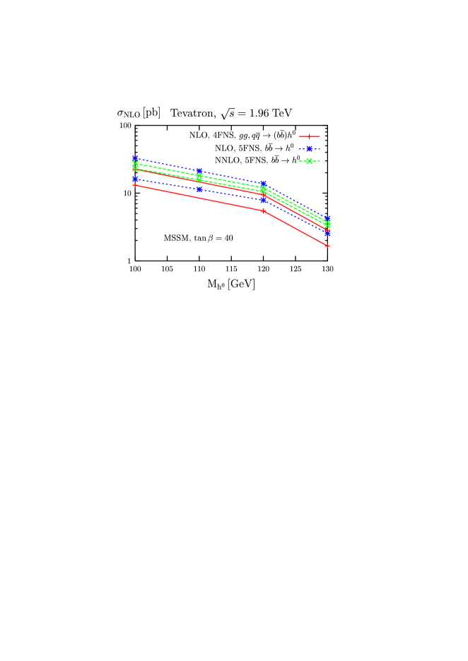
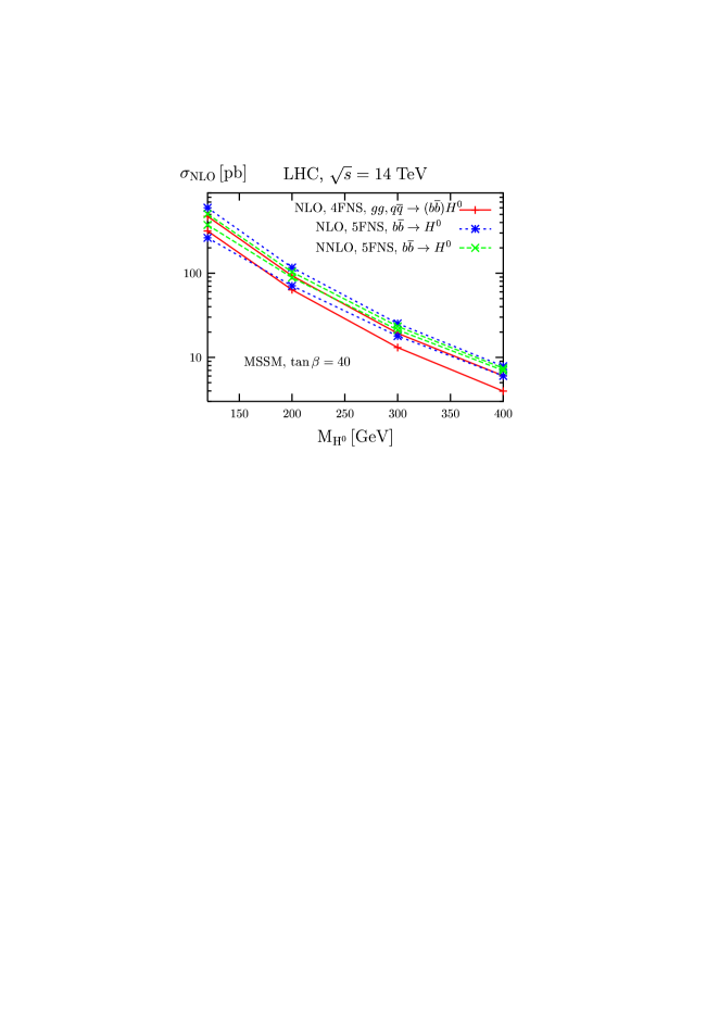
Figure 65: Total cross sections for $pp,p\bar{p}\rightarrow(b\bar{b})h$ ($h=h^{0},H^{0}$) in the MSSM with no bottom-quark jet identified in the final state in the 4FNS (at NLO) and 5FNS (at NLO and NNLO) as a function of the light and heavy MSSM Higgs boson masses, at both the Tevatron and the LHC. The error bands have been obtained by varying the renormalization ($\mu_{r}$) and factorization ($\mu_{f}$) scales separately between $\mu_{0}/4$ and $\mu_{0}$ (with $\mu_{0}\!=\!m_{b}+M_{H}/2$) in the 4FNS, while keeping $\mu_{r}\!=\!M_{h}$ and varying $\mu_{f}$ between $0.1M_{H}$ and $0.7M_{H}$ in the 5FNS (see Ref. Harlander:2003ai for details). From Ref. Dawson:2005vi .

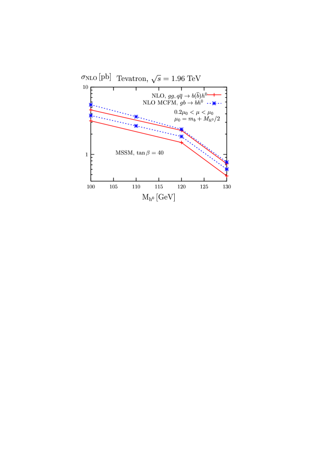
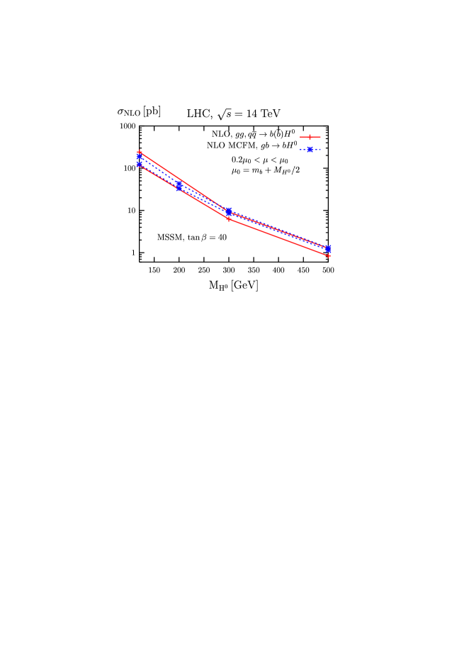
Figure 66: Total NLO cross section in the MSSM for $pp,p\bar{p}\rightarrow b(\bar{b})h$ production at the Tevatron and the LHC as a function of $M_{h^{0},H^{0}}$. We varied $\mu_{r}$ and $\mu_{f}$ independently to obtain the uncertainty bands, as explained in the text. The solid curves correspond to the 4FNS, the dashed curves to the 5FNS. The error bands have been obtained by varying the renormalization ($\mu_{r}$) and factorization ($\mu_{f}$) scales separately between $0.2\mu_{0}$ and $\mu_{0}$ (with $\mu_{0}\!=\!m_{b}+M_{H}/2$). From Ref. Dawson:2005vi .

It is actually very satisfactory that the NLO (and NNLO) calculations for the semi-inclusive and inclusive $b\bar{b}H$ production agree within their systematic errors. Indeed, if all perturbative orders were to be considered, the two approaches would produce the very same outcome. The truncation of the perturbative series at a given order gives origin to discrepancies, because the 4FNS and 5FNS perturbative series are differently ordered. However, we see that considering the first (second) order of corrections already brings the agreement between the two schemes within the respective theoretical uncertainties. The results shown in Figs. 66 and 65 represent indeed a major advancement, since the comparisons existing in the literature before Refs. Campbell:2004pu ; Dittmaier:2003ej ; Kramer:2004ie ; Dawson:2004sh showed a pronounced disagreement. This was mainly due to the absence of the (now available) NLO results for $q\bar{q},gg\rightarrow b\bar{b}H$.

References

- (1) F. Englert and R. Brout, Phys. Rev. Lett. 13, 321 (1964).
- (2) P. W. Higgs, Phys. Rev. Lett. 13, 508 (1964).
- (3) G. S. Guralnik, C. R. Hagen and T. W. B. Kibble, Phys. Rev. Lett. 13, 585 (1964).
- (4) M. E. Peskin and D. V. Schroeder, “An Introduction to quantum field theory”, Harper Collins Publishers (June 1, 1995)
- (5) S. Weinberg, “The Quantum theory of fields. Vol. 2: Modern Applications”, Cambridge University Press (August 13, 1996)
- (6) A. Djouadi, “The anatomy of electro-weak symmetry breaking. I: The Higgs boson in the standard model”, arXiv:hep-ph/0503172.
- (7) A. Djouadi, “The anatomy of electro-weak symmetry breaking. II: The Higgs bosons in the minimal supersymmetric model”, arXiv:hep-ph/0503173.
- (8) M. Carena and H. E. Haber, “Higgs boson theory and phenomenology”, Prog. Part. Nucl. Phys. 50, 63 (2003) [arXiv:hep-ph/0208209].
- (9) S. Dawson, “Introduction to the physics of Higgs bosons”, lectures given at TASI 94, arXiv:hep-ph/9411325.
- (10) S. Dawson, “Introduction to electroweak symmetry breaking”, lectures given at the 1998 ICTP Summer School in High-Energy Physics and Cosmology, arXiv:hep-ph/9901280.
- (11) CMS Collaboration, Technical Design Report, CERN/LHCC/94-38.
- (12) ATLAS Collaboration, Technical Design Report, Vol. II, Detector and physics performance, CERN/LHCC/99-15.
- (13) M. Carena et al. [Higgs Working Group Collaboration], arXiv:hep-ph/0010338.
- (14) D. Cavalli et al., arXiv:hep-ph/0203056.
- (15) L. Babukhadia et al. [CDF and D0 Working Group Members], FERMILAB-PUB-03-320-E
- (16) K. A. Assamagan et al. [Higgs Working Group Collaboration], arXiv:hep-ph/0406152.
- (17) T. Abe et al. [American Linear Collider Working Group], in Proc. of the APS/DPF/DPB Summer Study on the Future of Particle Physics (Snowmass 2001) ed. N. Graf, SLAC-R-570 Resource book for Snowmass 2001, 30 Jun - 21 Jul 2001, Snowmass, Colorado
- (18) J. A. Aguilar-Saavedra et al. [ECFA/DESY LC Physics Working Group], arXiv:hep-ph/0106315. arXiv:hep-ph/0106315.
- (19) LEP Electroweak Working Group, http://lepewwg.web.cern.ch/LEPEWWG/
- (20) LEP Higgs Working Group, http://lephiggs.web.cern.ch/LEPHIGGS/www/Welcome.html
- (21) [LEP Collaborations], arXiv:hep-ex/0412015.
- (22) [LEP Collaborations, SLD Collaboration, LEP EWWG, SLD EWWG and HFWG], arXiv:hep-ex/0509008.
- (23) t. L. E. Group [LEP Collaborations], arXiv:hep-ex/0511027.
- (24) R. Barate et al. [ALEPH Collaboration], Phys. Lett. B 565, 61 (2003) [arXiv:hep-ex/0306033].
- (25) [LEP Higgs Working Group], arXiv:hep-ex/0107030.
- (26) The LEP Higgs Working Group, LHWG-Note 2004-01.
- (27) K. Matchev, “TASI lectures on precision electroweak physics”, arXiv:hep-ph/0402031.
- (28) C. F. Kolda and H. Murayama, JHEP 0007, 035 (2000) [arXiv:hep-ph/0003170].
- (29) H. Haber, lectures presented at the TASI 2004 Summer Institute.
- (30) S. Heinemeyer, “MSSM Higgs physics at higher orders”, arXiv:hep-ph/0407244.
- (31) S. Heinemeyer, W. Hollik and G. Weiglein, “Electroweak precision observables in the minimal supersymmetric standard model”, arXiv:hep-ph/0412214.
- (32) A. Djouadi, J. Kalinowski and M. Spira, Comput. Phys. Commun. 108, 56 (1998) [arXiv:hep-ph/9704448].
- (33) M. Spira, Fortsch. Phys. 46, 203 (1998) [arXiv:hep-ph/9705337].
- (34) [LEP Higgs Working Group for Higgs boson searches], arXiv:hep-ex/0107031.
- (35) TeV4LHC Higgs Working Group, http://maltoni.home.cern.ch/maltoni/TeV4LHC/
- (36) S. Asai et al. (ATLAS Collaboration), Eur. Phys. J. C32S2, 19 (2004)
- (37) S. Abdullin et al. (CMS Collaboration), CMS Note 2003/33.
- (38) T. Affolder et al. [CDF Collaboration], Phys. Rev. Lett. 86, 4472 (2001) [arXiv:hep-ex/0010052].
- (39) V. M. Abazov et al. [D0 Collaboration], arXiv:hep-ex/0504018.
- (40) F. Gianotti and M. Pepe-Altarelli, Nucl. Phys. Proc. Suppl. 89, 177 (2000) [arXiv:hep-ex/0006016].
- (41) D. Zeppenfeld, R. Kinnunen, A. Nikitenko and E. Richter-Was, Phys. Rev. D 62, 013009 (2000) [arXiv:hep-ph/0002036].
- (42) A. Belyaev and L. Reina, JHEP 0208, 041 (2002) [arXiv:hep-ph/0205270].
- (43) M. Duhrssen, S. Heinemeyer, H. Logan, D. Rainwater, G. Weiglein and D. Zeppenfeld, Phys. Rev. D 70, 113009 (2004) [arXiv:hep-ph/0406323].
- (44) D. Wackeroth, lectures presented at the TASI 2004 Summer Institute.
- (45) S. Dawson, Nucl. Phys. B 359, 283 (1991).
- (46) A. Djouadi, M. Spira and P. M. Zerwas, Phys. Lett. B 264, 440 (1991).
- (47) C. J. Glosser and C. R. Schmidt, JHEP 0212, 016 (2002) [arXiv:hep-ph/0209248].
- (48) V. Ravindran, J. Smith and W. L. Van Neerven, Nucl. Phys. B 634, 247 (2002) [arXiv:hep-ph/0201114].
- (49) D. de Florian, M. Grazzini and Z. Kunszt, Phys. Rev. Lett. 82, 5209 (1999) [arXiv:hep-ph/9902483].
- (50) R. V. Harlander and W. B. Kilgore, Phys. Rev. Lett. 88, 201801 (2002) [arXiv:hep-ph/0201206].
- (51) C. Anastasiou and K. Melnikov, Nucl. Phys. B 646, 220 (2002) [arXiv:hep-ph/0207004].
- (52) C. Anastasiou, K. Melnikov and F. Petriello, arXiv:hep-ph/0409088.
- (53) V. Ravindran, J. Smith and W. L. van Neerven, Nucl. Phys. B 665, 325 (2003) [arXiv:hep-ph/0302135].
- (54) S. Catani, D. de Florian, M. Grazzini and P. Nason, JHEP 0307, 028 (2003) [arXiv:hep-ph/0306211].
- (55) G. Bozzi, S. Catani, D. de Florian and M. Grazzini, Phys. Lett. B 564, 65 (2003) [arXiv:hep-ph/0302104].
- (56) G. Bozzi, S. Catani, D. de Florian and M. Grazzini, arXiv:hep-ph/0508068.
- (57) W. Beenakker, S. Dittmaier, M. Kramer, B. Plumper, M. Spira and P. M. Zerwas, Phys. Rev. Lett. 87, 201805 (2001) [arXiv:hep-ph/0107081].
- (58) W. Beenakker, S. Dittmaier, M. Kramer, B. Plumper, M. Spira and P. M. Zerwas, Nucl. Phys. B 653, 151 (2003) [arXiv:hep-ph/0211352].
- (59) L. Reina and S. Dawson, Phys. Rev. Lett. 87, 201804 (2001) [arXiv:hep-ph/0107101].
- (60) L. Reina, S. Dawson and D. Wackeroth, Phys. Rev. D 65, 053017 (2002) [arXiv:hep-ph/0109066].
- (61) S. Dawson, L. H. Orr, L. Reina and D. Wackeroth, Phys. Rev. D 67, 071503 (2003) [arXiv:hep-ph/0211438].
- (62) S. Dawson, C. Jackson, L. H. Orr, L. Reina and D. Wackeroth, Phys. Rev. D 68, 034022 (2003) [arXiv:hep-ph/0305087].
- (63) R. M. Barnett, H. E. Haber and D. E. Soper, Nucl. Phys. B 306, 697 (1988).
- (64) F. I. Olness and W. K. Tung, Nucl. Phys. B 308, 813 (1988).
- (65) D. A. Dicus and S. Willenbrock, Phys. Rev. D 39, 751 (1989).
- (66) D. Dicus, T. Stelzer, Z. Sullivan and S. Willenbrock, Phys. Rev. D 59, 094016 (1999) [arXiv:hep-ph/9811492].
- (67) J. Campbell et al., arXiv:hep-ph/0405302.
- (68) S. Dittmaier, M. Kramer and M. Spira, Phys. Rev. D 70, 074010 (2004) [arXiv:hep-ph/0309204].
- (69) S. Dawson, C. B. Jackson, L. Reina and D. Wackeroth, Phys. Rev. D 69, 074027 (2004) [arXiv:hep-ph/0311067].
- (70) S. Dawson, C. B. Jackson, L. Reina and D. Wackeroth, Phys. Rev. Lett. 94, 031802 (2005) [arXiv:hep-ph/0408077].
- (71) M. Kramer, Nucl. Phys. Proc. Suppl. 135, 66 (2004) [arXiv:hep-ph/0407080].
- (72) J. Campbell, R. K. Ellis, F. Maltoni and S. Willenbrock, Phys. Rev. D 67, 095002 (2003) [arXiv:hep-ph/0204093].
- (73) R. V. Harlander and W. B. Kilgore, Phys. Rev. D 68, 013001 (2003) [arXiv:hep-ph/0304035].
- (74) S. Dawson, C. B. Jackson, L. Reina and D. Wackeroth, arXiv:hep-ph/0508293, to appear in Mod. Phys. Lett. A.