Mass and width of the lowest resonance in QCD

Abstract

We demonstrate that near the threshold, the $\pi\pi$ scattering amplitude contains a pole with the quantum numbers of the vacuum – commonly referred to as the $\sigma$ – and determine its mass and width within small uncertainties. Our derivation does not involve models or parametrizations, but relies on a straightforward calculation based on the Roy equation for the isoscalar $S$-wave.

According to the Particle Data Group, the lowest resonance in the spectrum of QCD carries angular momentum $\ell=0$ and isospin $I=0$. The state is listed as $f_{0}(600)$ and is usually called the $\sigma$. It manifests itself as a pole on the second sheet of the isoscalar $S$-wave of $\pi\pi$ scattering. We denote this partial wave amplitude by $t_{0}^{0}(s)$. The numbers for the pole position found in the literature cover a very broad range. For recent reviews, we refer to Ochs ; Pennington ; Bugg . In fact, since such a state is not easily accommodated in the multiplets expected for $q\bar{q}$ bound states and glueballs, some authors question its existence.

All of the pole determinations we are aware of rely on models and, moreover, use specific parametrizations to perform the analytic continuation. In the present paper, we instead rely on an equation which has been shown to follow from first principles, the dispersive representation of the partial wave amplitude $t^{0}_{0}(s)$ due to Roy Roy :

$$t_{0}^{0}(s) \!\!\!= \!\!\!a+(s-4M_{\pi}^{2})\,b+\int_{4M_{\pi}^{2}}^{\Lambda^{2}}\!\!ds^{\prime}\left\{K_{0}(s,s^{\prime})\,\mbox{Im}\,t_{0}^{0}(s^{\prime})\right.$$ (1)

$$\!\!\!\left.+\,K_{1}(s,s^{\prime})\,\mbox{Im}\,t_{1}^{1}(s^{\prime})+\,K_{2}(s,s^{\prime})\,\mbox{Im}\,t_{0}^{2}(s^{\prime})\right\}+d_{0}^{0}(s)\,.$$

It amounts to a twice subtracted dispersion relation. Crossing symmetry implies that both subtraction constants can be expressed in terms of the $S$-wave scattering lengths: $a=a_{0}^{0}$, $b=(2\,a_{0}^{0}-5\,a_{0}^{2})/(12M_{\pi}^{2})$. The integral describes the curvature generated by the $S$- and $P$-waves below $\Lambda$ and the so-called driving term $d_{0}^{0}(s)$ collects the dispersion integrals over the higher partial waves ($\ell\geq 2$), as well as the high energy end of the integral over the $S$- and $P$-waves.

Similar equations hold for all other partial waves. Those for the $S$- and $P$-waves amount to a set of coupled integral equations, which strongly constrain the low energy properties of these waves BFP ; ACGL ; CGL . Previous work on the Roy equations concerned the behaviour on the real axis. In Ref. CGL , a crude estimate of the mass and width of the $\sigma$ was given, but as emphasized in several reviews (see e.g. Ochs ; Pennington ), this estimate relies on a parametric extrapolation off the real axis and is thus subject to a sizeable systematic uncertainty.

The present paper closes this gap. We show that the domain of validity of the Roy equations can be extended to complex values of $s$ and use this extension to (a) prove the existence of a second sheet pole close to the threshold and (b) determine the position of this pole within rather small uncertainties. For this purpose, we only need the particular equation quoted above. The explicit expression for the kernels occurring therein reads:

$$K_{0}(s,s^{\prime}) = \frac{1}{\pi(s^{\prime}\!-\!s)}+\frac{2\,L}{3\pi(s\!-\!4M_{\pi}^{2})}-\frac{5s^{\prime}\!+\!2s\!-\!16M_{\pi}^{2}}{3\pi s^{\prime}(s^{\prime}\!-\!4M_{\pi}^{2})}\,,$$

$$K_{1}(s,s^{\prime}) = \frac{6(s^{\prime}\!+\!2s\!-\!4M_{\pi}^{2})\,L}{\pi(s^{\prime}\!-\!4M_{\pi}^{2})(s\!-\!4M_{\pi}^{2})}-\frac{3(2s^{\prime}\!+\!3s\!-\!4M_{\pi}^{2})}{\pi s^{\prime}(s^{\prime}\!-\!4M_{\pi}^{2})}\,,$$

$$K_{2}(s,s^{\prime}) = \frac{10\,L}{3\pi(s\!-\!4M_{\pi}^{2})}-\frac{5(2s^{\prime}\!-\!s\!-\!4M_{\pi}^{2})}{3\pi s^{\prime}(s^{\prime}\!-\!4M_{\pi}^{2})}\,,$$

$$\mbox{where}\hskip 10.00002ptL=\ln\left(\frac{s+s^{\prime}-4M_{\pi}^{2}}{s^{\prime}}\right)\;\;.$$

The first term in $K_{0}(s,s^{\prime})$ accounts for the contributions generated by the right hand cut. The remainder of $K_{0}(s,s^{\prime})$ describes those contributions from the left hand cut that are also due to $\mbox{Im}\,t_{0}^{0}$, while those from $\mbox{Im}\,t_{1}^{1}$ ($P$-wave) and $\mbox{Im}\,t_{0}^{2}$ (exotic $S$-wave) are booked separately.

For our analysis, it is essential that the dispersion integral is dominated by the contributions from the low energy region: because the Roy equations involve two subtractions, the kernels $K_{n}(s,s^{\prime})$ fall off in proportion to $1/s^{\prime\,3}$ for large $s^{\prime}$. Note that the contributions from the left hand cut play an important role here: Dropping these, $K_{0}(s,s^{\prime})$ reduces to the first term, which falls off only with the first power of $s^{\prime}$. Taken by itself, the contribution from the right hand cut is therefore sensitive to the poorly known high energy behaviour of $\mbox{Im}\,t_{0}^{0}(s^{\prime})$, but taken together with the one from the left hand cut, the high energy tails cancel.

Since the decomposition into partial waves is useful only at low energies, the dispersion integral over the $S$- and $P$-waves in Eq. (1) is cut off, the high energy tail being included in $d^{0}_{0}(s)$. As discussed in Ref. ACGL , $d^{0}_{0}(s)$ is dominated by the contribution from the

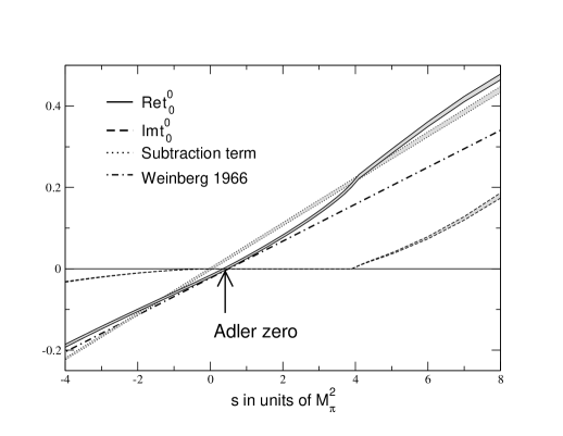
Figure 1: Behaviour of the amplitude near threshold.

$D$-wave resonance $f_{2}(1270)$. Using the narrow width approximation, expanding the relevant kernel in inverse powers of $s^{\prime}=M_{f_{2}}^{2}$ and retaining only the leading term of order $1/s^{\prime\,3}$, we obtain

$$d_{0}^{\hskip 0.35002pt0}(s)\simeq\frac{5(s-4M_{\pi}^{2})(11s+4M_{\pi}^{2})\,\Gamma_{f_{2}\rightarrow\pi\pi}}{9M_{f_{2}}^{4}\sqrt{\rule{0.0pt}{10.00002pt}M_{f_{2}}^{2}-4M_{\pi}^{2}}}\;\;.$$ (3)

The experimental values for mass and width are $M_{f_{2}}=1275.4\pm 1.2$ MeV, $\Gamma_{f_{2}\rightarrow\pi\pi}=158.5\pm 4.4$ MeV PDG 2004 .

We have performed a detailed evaluation of the driving term, which exploits the Roy equations for the $D$-, $F$- and $G$-waves and accounts for the contributions from the high energy tail. The calculation shows that, in the low energy region we are considering in the present paper, the contributions from partial waves with $\ell>2$ as well as those from energies above 1.4 GeV are negligibly small and the narrow width approximation works: for $\Lambda\geq 1.4$ GeV, the above simple formula is within the uncertainties attached to the full result, which affect the outcome for the pole position only by 1 or 2 MeV.

The most important feature in the low energy region is the occurrence of an Adler zero. To leading order of chiral perturbation theory, the amplitude is given by Weinberg’s formula of 1966 Weinberg 1966 ,

$$t_{0}^{0}(s)=(2s-M_{\pi}^{2})/(32\pi F_{\pi}^{2})\;\;.$$ (4)

In this approximation, the zero occurs at $s=\frac{1}{2}M_{\pi}^{2}$. Fig.1 shows the behaviour of the amplitude – calculated from Eq. (1) – near the threshold and explains why the theoretical predictions are so precise in this region: by far the most important contribution stems from the subtraction term, which is linear in $s$ and is fixed by the two scattering lengths $a_{0}^{0}$, $a_{0}^{2}$. Accordingly, the values of $a_{0}^{0}$ and $a_{0}^{2}$ represent the most important ingredient of our calculation. Since theory predicts these very accurately CGL ,

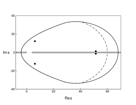
Figure 2: Domain of validity of the Roy equations.

$$a_{0}^{0}=0.220\pm 0.005\;\;,\hskip 10.00002pta_{0}^{2}=-0.0444\pm 0.0010\;\;,$$ (5)

the uncertainties in the subtraction term are very small. The main experiments concerning the scattering lengths E865 ; DIRAC ; NA48 are all in good agreement with these predictions, but provide a stringent test only for the first one. On the other hand, as will be discussed below, the experimental information does suffice to evaluate the dispersion integrals in Eq.(1) to good accuracy.

The Roy equations represent the partial wave projections of the fixed-$t$ dispersion relations obeyed by the $\pi\pi$ scattering amplitude. These relations are valid if the variable $t$ is contained in a Lehmann-Martin ellipse with foci at $t=0$ and $t=4\,M_{\pi}^{2}-s^{\prime}$ and right extremity at $t=r(s^{\prime})$, where $s^{\prime}\geq 4\,M_{\pi}^{2}$ is the variable of integration. In the Mandelstam representation, the size of the ellipse is limited by the singularities due to the double spectral function. For $4\,M_{\pi}^{2}\leq s^{\prime}\leq 20\,M_{\pi}^{2}$, the corresponding expression for $r(s^{\prime})$ reads $r(s^{\prime})=16\,s^{\prime}/(s^{\prime}-4\,M_{\pi}^{2})$, while for $s^{\prime}>20\,M_{\pi}^{2}$, the right extremity is at $r(s^{\prime})=4\,s^{\prime}/(s^{\prime}-16\,M_{\pi}^{2})$.

The partial wave projection involves the values of the amplitude on the interval $t=\frac{1}{2}\,(4\,M_{\pi}^{2}-s)(1-z)$, $0\leq z\leq 1$. For the Roy equations to be valid at the point $s$, the corresponding interval must be contained in the intersection of the ellipses characterized above. The boundary of the domain $G$ where this is the case is shown as a solid line in fig. 2, using pion mass units. The bound for $r(s^{\prime})$ established on the basis of axiomatic field theory Martin book ; Mahoux is only slightly weaker. The dash-dotted line indicates the corresponding domain of validity of the Roy equations. On the real axis, this domain reduces to the range $-4\,M_{\pi}^{2}<s<60\,M_{\pi}^{2}$ obtained in Ref. Roy .

The values of the $S$-matrix element

$$S^{0}_{0}(s)=1-2\sqrt{4\,M_{\pi}^{2}/s-1}\;t_{0}^{0}(s)$$ (6)

on the second sheet can be calculated from those on the first sheet: unitarity implies the relation Unitarity

$$S_{0}^{0}(s)^{II}=1/S_{0}^{0}(s)^{I}\;\;.$$ (7)

The Roy equation thus automatically also specifies the function $S_{0}^{0}(s)$ on the second sheet, in the same domain of the $s$-plane bachir . In particular, the amplitude contains a pole on the second sheet if and only if $S_{0}^{0}(s)$ has a zero on the physical sheet. So, all we need to do is numerically evaluate Eq. (1) for complex values of $s$ in the domain $G$ where it has been shown to hold and find out whether or not $S_{0}^{0}(s)$ has zeros there – standard routines that solve equations numerically immediately provide the answer.

As discussed in Ref. CGL , the Roy equations for the $S$ and $P$-waves provide very firm control over the low energy behaviour of the imaginary parts occurring in Eq.(1). The numbers given in the following are based on a new analysis of these equations which will be described elsewhere. We could just as well have used the results in Ref. CGL – the numbers would barely change. For our central representation of the scattering amplitude, the function $S_{0}^{0}(s)$ has two pairs of zeros in $G$, one at $s=(6.2\pm i\,12.3)\,M_{\pi}^{2}$, the other at $s=(51.4\pm i\,1.4)\,M_{\pi}^{2}$. These are indicated in fig. 2, which may also be viewed as a picture of the second sheet – the dots then represent poles rather than zeros. In the following, we work with the complex mass $m_{\sigma}\equiv M_{\sigma}-\frac{i}{2}\,\Gamma_{\sigma}$, defined as the value of $\sqrt{s}$ at the pole on the lower half of the second sheet. For the central solution, the pole occurs at $m_{\sigma}=441-i\,272$ MeV, not far from the place where the $\sigma$ was resurrected ten years ago Tornqvist and Roos .

The second pole represents the well-established resonance $f_{0}(980)$. In order to study the behaviour of the amplitude there, we have extended the analysis of Refs. ACGL ; CGL to higher energies. The BES data on the decay $J/\psi\rightarrow\phi\pi\pi$ BES f0(980) have clarified the structure in this region. In this reference, the sharp drop in the elasticity $\eta 0_{0}(s)$ at the $K\bar{K}$ threshold is parametrized by means of the so-called Flatté formula, which describes the interference between the $K\bar{K}$ cut and the pole from the $f_{0}(980)$. Given the elasticity, the Roy equations determine the phase shift. It turns out that the solution closely follows the input: the phase shift differs from the phase of the Flatté formula only by a slowly varying background. It does not come as a surprise, therefore, that our calculation confirms the position of the pole in BES f0(980) and we do not discuss this further.

Finally, we estimate the uncertainty to be attached to the result obtained from our central representation of the scattering amplitude. The Roy equations imply that if the two subtraction constants $a_{0}^{0}$ and $a_{0}^{2}$ are treated as known, the low energy properties of the isoscalar $S$-wave depend almost exclusively on a single parameter, which may be identified with the value of the phase at 800 MeV and which we denote by $\delta_{A}\equiv\delta_{0}^{0}(800\,\mbox{MeV})$. Accordingly, it is convenient to represent the position of the pole as

$$m_{\sigma} \!\!\!= \!\!\!m_{0}+m_{1}\,\Delta a_{0}^{0}+m_{2}\,\Delta a_{0}^{2}+m_{3}\,\Delta\delta_{A}\,,$$ (8)

$$\Delta a_{0}^{0} \!\!\!= \!\!\!(a_{0}^{0}-0.22)/0.005\,,\;\Delta a_{0}^{2}=(a_{0}^{2}+0.0444)/0.001\,,$$

$$\Delta\delta_{A} \!\!\!= \!\!\!(\delta_{A}-82.3)/3.4\,.$$

The term $m_{0}$ represents the value of the complex mass obtained if the scattering lengths are fixed at the central values of the prediction (5), while the phase at 800 MeV is set equal to the central value obtained from the phenomenology of the phase difference between $\delta_{1}^{1}$ and $\delta_{0}^{0}$ ACGL . The coefficients $m_{1}$, $m_{2}$ and $m_{3}$ describe the sensitivity of the result to a change in these variables – for the small changes of interest, the linear approximation is adequate.

The residual noise in $m_{0}$ is small, for the following reasons. (a) The integral over $\mbox{Im}\,t^{0}_{0}$ is dominated by the region below the $K\bar{K}$ threshold. If $a_{0}^{0}$, $a_{0}^{2}$ and $\delta_{A}$ are held fixed, the Roy equations constrain the integrand very strongly there. (b) The contribution from the $P$-wave is dominated by the $\rho$. Since the experimental information about this state is excellent, the integral over $\mbox{Im}\,\,t_{1}^{1}$ is known very well. (c) In $\mbox{Im}\,t^{2}_{0}$, the uncertainties are larger, but the entire contribution from this wave is small. (d) As stated above, the uncertainties in the higher partial waves and in the contributions from the high energy tail of the dispersion integrals affect the result for $m_{\sigma}$ only at the level of 1 or 2 MeV. In our opinion, the estimate $m_{0}=(441\pm 4)-i\,(272\pm 6)$ MeV generously covers the uncertainties. For the other coefficients in Eq. (8), we obtain $m_{1}=-2.4+i\,3.8$, $m_{2}=0.8-i\,4.0$, $m_{3}=5.3+i\,3.3$ (values in MeV).

The result for the pole position does not change significantly if the imaginary parts are evaluated with a phenomenological representation of the data. We illustrate this with the parametrization of the scattering amplitude proposed in appendix A of Ref. PY . Evaluating the dispersion integrals over $\mbox{Im}\,t_{0}^{0}$, $\mbox{Im}\,t_{1}^{1}$ and $\mbox{Im}\,t_{0}^{2}$ with the central parametrization of that reference, we find that the pole occurs at $445-i\,241$ MeV. Although this representation differs significantly from our central solution, the result for the pole position agrees with formula (8): for the values $a_{0}^{0}=0.23$, $a_{0}^{2}=-0.048$ and $\delta_{A}=90.9^{\circ}$ that correspond to this parametrization, the formula yields $m_{\sigma}=447-i\,242$ MeV.

This confirms that the position of the pole from the $\sigma$ is indeed controlled by three observables. Only one of these, $a_{0}^{0}$, is known experimentally to good precision. For the second one, $a_{0}^{2}$, the sharp theoretical prediction in Eq. (5) was recently confirmed by an evaluation on the lattice: $a^{2}_{0}=-0.0426(6)(3)(18)$, where the three brackets give the statistical, systematic and theoretical errors, respectively Beane (cf. also Yamazaki:2004qb ). To stay on the conservative side with the third parameter, we use $\delta_{A}=82.3^{\circ}\stackrel{{\scriptstyle+10^{\circ}}}{{{}_{-4^{\circ}}}}$. Compared to the uncertainty from this source, the noise in the term $m_{0}$ is negligible. With the theoretical prediction for the scattering lengths, formula (8) then leads to our final result

$$M_{\sigma}=441\stackrel{{\scriptstyle+16}}{{{}_{-8}}}\,\mbox{MeV}\,,\;\;\Gamma_{\sigma}=544\stackrel{{\scriptstyle+18}}{{{}_{-25}}}\,\mbox{MeV}\;\;.$$ (9)

We conclude that the same theoretical framework that leads to incredibly sharp predictions for the threshold parameters of $\pi\pi$ scattering CGL also requires the occurrence of a pole on the lower half of the second sheet, with the quantum numbers of the vacuum, not much above the threshold, but quite far from the real axis: the width of the $\sigma$ is larger than the width of the $\rho$ by a factor of 3.7. The parametric extrapolation used in Ref. CGL led to somewhat higher values, for the mass as well as for the width – the difference amounts to about 1 standard deviation. The uncertainty in the result (9) stems almost exclusively from $\delta_{A}$. The range adopted for this observable covers all of the phenomenological parametrizations we are aware of. (Energy-independent analyses have a broader scatter of values, but even the most extreme Kaminski:2001hv is less than $2\,\sigma$ away from our central value.) It can be reduced substantially if the data that underly these parametrizations are compared with the solutions of the Roy equations. We intend to describe this elsewhere.

The experimental information concerning $a_{0}^{2}$ is meagre, but since the real part of the coefficient $m_{2}$ is very small, this does not affect the value of $M_{\sigma}$: as far as the real part of the pole position is concerned, the result remains practically unchanged if the theoretical predictions for the scattering lengths are replaced by the experimental constraints on these E865 ; DIRAC ; NA48 .

Many of the determinations of the mass and width of the $\sigma$ listed by the Particle Data Group neglect the left hand cut. In the language of Eq. (1), this approximation amounts to replacing the kernel $K_{0}$ by the first term in Eq. (Mass and width of the lowest resonance in QCD) and dropping $K_{1}$, $K_{2}$ as well as $d_{0}^{0}$. For definiteness, we fix the subtraction constants $a$ and $b$ such that the “exact” and approximate representations agree at the threshold and at $\sqrt{s_{A}}=800\,\mbox{MeV}$. At the energies of interest, the difference is then well described by the parabola $t_{0}^{0}(s)_{\mbox{lhc}}\simeq c\,(s-4\,M_{\pi}^{2})(s_{A}-s)$, with $c=0.5\,\mbox{GeV}^{-4}$. Removing this term from $t_{0}^{0}(s)$ has a rather drastic effect: the pole then occurs at $m_{\sigma}\simeq 500-i\,260$ MeV. The amplitude obtained in this manner cannot be taken at face value, because it violates unitarity: dropping the left hand cut necessarily also distorts the imaginary part. We do not pursue this further. The above expression for the corresponding curvature shows that the left hand cut cannot be neglected – the pole is not sufficiently far away from it for this approximation to be meaningful.

It is difficult to understand the properties of the lowest resonances in terms of the degrees of freedom of the quarks and gluons. The physics of the $\sigma$ is governed by the dynamics of the Goldstone bosons: The properties of the interaction among two pions are relevant Markushin and Locher . A qualitative explanation for the occurrence of the $\sigma$ was given in Ref. CGL , on the basis of current algebra, spontaneous symmetry breakdown and unitarity. The properties of the resonance $f_{0}(980)$ are also governed by Goldstone boson dynamics – two kaons in that case. It would be of considerable interest to apply the above analysis to the Roy-Steiner equation Buettiker Descotes Moussallam for the $K\pi$ $S$-wave with $I=\frac{1}{2}$. This should clarify the situation with the $\kappa$.

- (1) W. Ochs, in Hadron Spectroscopy: Tenth International Conference, edited by E. Klempt, H. Koch and H. Orth, AIP Conf. Proc. No. 717 (AIP, New York, 2004), p. 295.
- (2) M. R. Pennington, arXiv:hep-ph/0509265.
- (3) D. V. Bugg, in Hadron Spectroscopy: Eleventh International Conference on Hadron Spectroscopy, edited by A. Reis, C. Göbel, J. de Sá Borges and J. Magnin, AIP Conf. Proc. No. 814 (AIP, New York, 2006), p. 78.
- (4) S. M. Roy, Phys. Lett. B 36 (1971) 353.
- (5) J. L. Basdevant, C. D. Froggatt and J. L. Petersen, Nucl. Phys. B 72 (1974) 413.
- (6) B. Ananthanarayan, G. Colangelo, J. Gasser and H. Leutwyler, Phys. Rept. 353 (2001) 207.
- (7) G. Colangelo, J. Gasser and H. Leutwyler, Nucl. Phys. B 603 (2001) 125.
- (8) S. Eidelman et al. [Particle Data Group], Phys. Lett. B 592 (2004) 1.
- (9) S. Weinberg, Phys. Rev. Lett. 17 (1966) 616.
- (10) S. Pislak et al. [BNL-E865 Collaboration], Phys. Rev. Lett. 87 (2001) 221801 Phys. Rev. D 67 (2003) 072004.
- (11) B. Adeva et al. [DIRAC Collaboration], Phys. Lett. B 619 (2005) 50.
- (12) J. R. Batley et al. [NA48/2 Collaboration], Phys. Lett. B 633 (2006) 173.
- (13) A. Martin, Scattering Theory: Unitarity, Analyticity and Crossing, Lecture Notes in Physics, Vol. 3, (Springer-Verlag, Berlin, 1969).
- (14) G. Mahoux, S. M. Roy and G. Wanders, Nucl. Phys. B 70 (1974) 297.
- (15) For a derivation, see for instance Ref. BFP
- (16) We thank Bachir Moussallam for this remark.
- (17) N. A. Tornqvist and M. Roos, Phys. Rev. Lett. 76 (1996) 1575.
- (18) M. Ablikim et al. [BES Collaboration], Phys. Lett. B 607 (2005) 243.
- (19) J. R. Peláez and F. J. Ynduráin, Phys. Rev. D 71 (2005) 074016.
- (20) S. R. Beane, P. F. Bedaque, K. Orginos and M. J. Savage [NPLQCD Collaboration], hep-lat/0506013.
- (21) T. Yamazaki et al. [CP-PACS Collaboration], Phys. Rev. D 70 (2004) 074513.
- (22) R. Kaminski, L. Lesniak and K. Rybicki, Eur. Phys. J. directC 4 (2002) 1.
- (23) V. E. Markushin and M. P. Locher, in Workshop in Hadron Spectrocopy, Frascati Physics Series, Vol. XV (Laboratori Nazionali di Frascati, Rome, 1999), p. 229.
- (24) P. Buettiker, S. Descotes-Genon and B. Moussallam, Eur. Phys. J. C 33 (2004) 409.