Enhanced $\mu^{-}-e^{-}$ conversion in nuclei in the inverse seesaw model

Abstract

We investigate nuclear $\mu^{-}-e^{-}$ conversion in the framework of an effective Lagrangian arising from the inverse seesaw model of neutrino masses. We consider lepton flavour violation interactions that arise from short range (non-photonic) as well as long range (photonic) contributions. Upper bounds for the $L_{f}/\hskip 5.0pt$ - parameters characterizing $\mu^{-}-e^{-}$ conversion are derived in the inverse seesaw model Lagrangian using the available limits on the $\mu^{-}-e^{-}$ conversion branching ratio, as well as the expected sensitivities of upcoming experiments. We comment on the relative importance of these two types of contributions and their relationship with the measured solar neutrino mixing angle $\theta_{12}$ and the dependence on $\theta_{13}$. Finally we show how the $L_{f}/\hskip 5.0pt$ $\mu^{-}-e^{-}$ conversion and the $\mu^{-}\to e^{-}\gamma$ rates are strongly correlated in this model.

I Introduction

The discovery of neutrino oscillations fukuda:1998mi ; ahmad:2002jz ; eguchi:2002dm shows that neutrinos are massive Maltoni:2004ei and that lepton flavour is violated in neutrino propagation. The violation of this conservation law could show up in other contexts, such as rare lepton flavour violating (LFV) decays of muons and taus, e.g. $\mu^{-}\to e^{-}\gamma$. In fact, there are strong indications from theory that this may be the case. Among the lepton flavour violating ($L_{f}/\hskip 5.0pt$ ) processes, the electron- and muon-flavour violating nuclear conversion

$$\mu^{-}+(A,Z)\longrightarrow e^{-}\,+\,(A,Z)^{*}\,,$$ (1)

is known to provide a very sensitive probe of lepton flavour violation Hisano:1995cp ; Kosmas:1993ch ; Kosmas:1990tc ; Kosmas:2001mv ; Kosmas:2001ia ; faessler:2000pn ; Kitano:2003wn . This follows from the distinct feature of a coherent enhancement in nuclear $\mu^{-}-e^{-}$ conversion. From the experimental viewpoint, currently the best upper bound on the $\mu^{-}-e^{-}$ conversion branching ratio comes from the SINDRUM II experiment at PSI vanderSchaaf:2003ti , using ¹⁹⁷Au as stopping target,

$$R_{\mu e}^{Au}\leq 5.0\times 10^{-13}\ \ \ \ \rm{90\%C.L.}\ \ \$$ (2)

The proposed aim of the MECO experiment, the $\mu^{-}-e^{-}$ conversion experiment at Brookhaven Molzon:1998kg , with ²⁷Al as target is expected to reach Molzon:1998kg

$$R_{\mu e}^{Al}\leq 2\times 10^{-17}\ \ \ \ \ \ \ \$$ (3)

about three to four orders of magnitude better than the present best limit.

An even better sensitivity is expected at the new $\mu^{-}-e^{-}$ conversion PRISM experiment at Tokyo, with ⁴⁸Ti as stopping target. This experiment aims at Kuno:2000kd

$$R_{\mu e}^{Ti}\leq 10^{-18}.$$ (4)

Such an impressive sensitivity can place severe constraints on the underlying parameters of $\mu^{-}-e^{-}$ conversion.

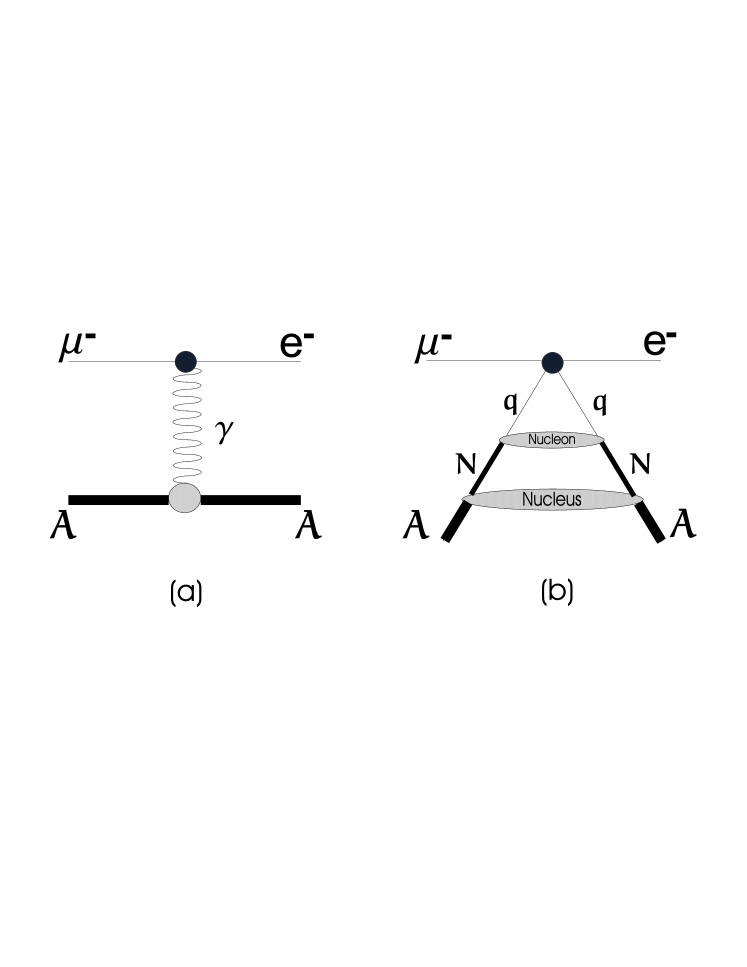
There are many mechanisms beyond the Standard Model that could lead to lepton flavour violation (see Kosmas:1993ch ; Hisano:1995cp ; Kosmas:1990tc ; Kosmas:2001ia ; faessler:2000pn and references therein). The corresponding Feynman diagrams can be classified according to their short-range or long-range character into two types: photonic and non-photonic, as shown in Fig. 1. The long-distance photonic mechanisms in Fig. 1(a) are mediated by virtual photon exchange between nucleus and the $\mu-e$ lepton current. The hadronic vertex is characterized in this case by ordinary electromagnetic nuclear form factors. Contributions to $\mu-e$ conversion arising from virtual photon exchange are generically correlated to $\mu\to e\gamma$ decay.

The short-distance non-photonic mechanisms in Fig. 1(b) include effective 4-fermion quark-lepton $L_{f}/\hskip 5.0pt$ interactions which couple the quarks and leptons via heavy intermediate particles ($W,Z$, Higgs bosons, supersymmetric particles, etc.) at the tree level, at the 1-loop level or via box diagrams. The various mechanisms can significantly differ in many respects, in particular, in what concerns nucleon and nuclear structure treatment. As a result, they must be treated on a case-by-case basis.

In this paper we consider $\mu^{-}-e^{-}$ conversion in the context of a variant of the seesaw model Minkowski:1977sc , called inverse seesaw mohapatra:1986bd . It differs from the standard one in that no large mass scale is necessary, providing a simple framework for enhanced $L_{f}/\hskip 5.0pt$ rates, unsuppressed by small neutrino masses bernabeu:1987gr ; branco:1989bn . The enhancement of $L_{f}/\hskip 5.0pt$ rates holds in this model even in the absence of supersymmetry and in the absence of neutrino masses. For this reason it plays a special role. For simplicity here we neglect possible supersymmetric contributions to the $L_{f}/\hskip 5.0pt$ rates that could exist in this model, see Deppisch:2004fa . Other seesaw constructions with extended gauge groups have been considered recently, using either left–right gauge symmetry Akhmedov:1995vm or full SO(10) unification Barr:2005ss ; Fukuyama:2005gg ; Malinsky:2005bi . They, too, will lead to enhanced LFV rates. However, both for definiteness and simplicity, here we focus our discussion on the case of the simplest SU(2) $\otimes$ U(1) inverse seesaw model which we take as a reference model. First, we derive a formula for the $\mu^{-}-e^{-}$ conversion branching ratio in terms of $L_{f}/\hskip 5.0pt$ parameters of the effective Lagrangian of the model. The transformation of this Lagrangian, first to the nucleon and then to the nuclear level, needs special attention to the effects of nucleon and nuclear structure. The nucleon structure is taken into account on the basis of the QCD picture of baryon masses and experimental data on certain hadronic parameters. The nuclear physics, which is involved in the muon-nucleus overlap integrals faessler:2000pn ; Schwieger:1998dd is evaluated paying special attention on specific nuclei that are of current experimental interest like, ²⁷Al, ⁴⁸Ti and ¹⁹⁷Au.

Figure 1: (a) Photonic (long-distance) and (b) non-photonic (short-distance) contributions to the nuclear $\mu^{-}-e^{-}$ conversion.

II Inverse seesaw mechanism

The model extends minimally the particle content of the Standard Model by the sequential addition of a pair of two-component SU(2) $\otimes$ U(1) singlet leptons, as follows

$$\left(\begin{array}[]{c}\nu_{i}\\ e_{i}\\ \end{array}\right),e_{i}^{c},\nu_{i}^{c},S_{i},$$ (5)

with $i$ a generation index running over $1,2,3$. In addition to the more familiar right-handed neutrinos characteristic of the standard seesaw model, the inverse seesaw scheme contains an equal number of gauge singlet neutrinos $S_{i}$. In the original formulation of the model, these were superstring inspired $E(6)$ singlets, in contrast to the right-handed neutrinos, members of the spinorial representation. Recently similar constructions have been considered in the framework of left–right symmetry Akhmedov:1995vm or SO(10) unified models Malinsky:2005bi ; Barr:2005ss ; Fukuyama:2005gg .

In the $\nu,\nu^{c},S$ basis, the $9\times 9$ neutral leptons mass matrix $\mathcal{M}$ is given as

$${\mathcal{M}}=\left(\begin{array}[]{ccc}0&m_{D}^{T}&0\\ m_{D}&0&M^{T}\\ 0&M&\mu\end{array}\right),$$ (6)

where $m_{D}$ and $M$ are arbitrary $3\times 3$ complex matrices in flavour space, whereas $\mu$ is complex symmetric. The matrix $\mathcal{M}$ can be diagonalized by a unitary mixing matrix $U_{\nu}$,

$$U_{\nu}^{T}{\mathcal{M}}U_{\nu}=\mathrm{diag}(m_{i},M_{4},...,M_{9}),$$ (7)

yielding 9 mass eigenstates $n_{a}$. In the limit of small $\mu$ three of these correspond to the observed light neutrinos with masses $m_{i}$, while the three pairs of two-component leptons $(\nu^{c}_{i},S_{i})$ combine to form three heavy leptons, of the quasi-Dirac type valle:1983yw .

The light neutrino mass states $\nu_{i}$ are given in terms of the flavour eigenstates via the unitary matrix $U_{\nu}$

$$\nu_{i}=\sum_{a=1}^{9}(U_{\nu})_{ia}n_{a}.$$ (8)

which has been studied in earlier papers bernabeu:1987gr ; branco:1989bn . The diagonalization results in an effective Majorana mass matrix for the light neutrinos gonzalez-garcia:1989rw ,

$$m_{\nu}={m_{D}^{T}M^{T}}^{-1}\mu M^{-1}m_{D},$$ (9)

where we are assuming $\mu,m_{D}\ll M$. One sees that the neutrino masses vanish in the limit $\mu\to 0$ where lepton number conservation is restored. In models where lepton number is spontaneously broken by a vacuum expectation value $\left\langle\sigma\right\rangle$ gonzalez-garcia:1989rw one has $\mu=\lambda\left\langle\sigma\right\rangle$. Typical parameter values may be estimated from the required values of the light neutrino masses indicated by oscillation data Maltoni:2004ei as

$$\left(\frac{m_{\nu}}{0.1\mathrm{eV}}\right)=\left(\frac{m_{D}}{100\mathrm{GeV}}\right)^{2}\left(\frac{\mu}{1\mathrm{keV}}\right)\left(\frac{M}{10^{4}\mathrm{GeV}}\right)^{-2},$$ (10)

For typical Yukawas $\lambda\sim 10^{-3}$ one sees that $\mu=1$ keV corresponds to a low scale of L violation, $\left\langle\sigma\right\rangle\sim 1$ MeV (for very low values of $\left\langle\sigma\right\rangle$ this might lead to interesting signatures in neutrinoless double beta decays berezhiani:1992cd ) .

In contrast, in the conventional seesaw mechanism without the gauge singlet neutrinos $S_{i}$ one would have

$$\left(\begin{array}[]{cc}0&m_{D}^{T}\\ m_{D}&M_{R}\end{array}\right),\qquad m_{D}\ll M_{R}\Rightarrow m_{\nu}=m_{D}^{T}M_{R}^{-1}m_{D}\,.$$ (11)

Note that in the “inverse seesaw” scheme the three pairs of singlet neutrinos have masses of the order of $M$ and their admixture in the light neutrinos is suppressed as $\frac{m_{D}}{M}$. It is crucial to realize that the mass $M$ of our heavy leptons can be much smaller than the $M_{R}$ characterizing the right-handed neutrinos in the conventional seesaw, since the suppression in Eq. (10) is quadratic in $M^{-1}$ (as opposed to the linear dependence in $M_{R}^{-1}$ given by Eq. (11)), and since we have the independent small parameter $\mu$ characterizing the lepton number violation scale. As a result the value of $M$ may be as low as the weak scale (if light enough, these neutral leptons could give signatures at accelerator experiments Dittmar:1990yg ; Abreu:1997pa ).

Without loss of generality one can assume $\mu$ to be diagonal,

$$\mu=\hbox{diag}\;\mu_{i},$$ (12)

and using the diagonalizing matrix $U$ of the effective light neutrino mass matrix $m_{\nu}$,

$$U^{T}m_{\nu}U=\hbox{diag}\;m_{i},$$ (13)

equation (9) can be written as

$$\mathbf{1}=\hbox{diag}\;\sqrt{m_{i}^{-1}}\cdot U^{T}m_{D}^{T}{M^{T}}^{-1}\cdot\hbox{diag}\;\sqrt{\mu_{i}}\cdot\hbox{diag}\;\sqrt{\mu_{i}}\cdot M^{-1}m_{D}U\cdot\hbox{diag}\;\sqrt{m_{i}^{-1}}.$$ (14)

In the basis where the charged lepton Yukawa couplings are diagonal the lepton mixing matrix is simply the rectangular matrix formed by the first three rows of $U_{\nu}$ schechter:1980gr .

In analogy to the standard seesaw mechanism Casas:2001sr it is thus possible to define a complex orthogonal matrix

$$R=\hbox{diag}\;\sqrt{\mu_{i}}\cdot M^{-1}m_{D}U\cdot\hbox{diag}\;\sqrt{m_{i}^{-1}}$$ (15)

with 6 real parameters. Using $R$, the neutrino Yukawa coupling matrix $Y_{\nu}=\frac{1}{v\sin\beta}m_{D}$ can be expressed as

$$Y_{\nu}=\frac{1}{v\sin\beta}M\cdot\hbox{diag}\;\sqrt{\mu_{i}^{-1}}\cdot R\cdot\hbox{diag}\;\sqrt{m_{i}}\cdot U^{\dagger},$$ (16)

To further simplify our discussion we make the assumption that the eigenvalues of both $M$ and $\mu$ are degenerate and that $R$ is real. This allows us to easily compare our results with those obtained previously in Ref. Deppisch:2002vz ; Deppisch:2003wt for the case of the conventional seesaw mechanism.

III The effective quark-level Lagrangian

In our model the $L_{f}/\hskip 5.0pt$ arises from penguin photon and Z exchange as well as box diagrams, as illustrated in Fig. 2. The resulting effective Lagrangian can be expressed as Hisano:1995cp

$${\mathcal{L}}_{eff} = {\mathcal{L}}_{eff}^{\gamma}+{\mathcal{L}}_{eff}^{Z}+{\mathcal{L}}_{eff}^{box}$$ (17)

$${\mathcal{L}}_{eff}^{\gamma} = -\frac{e^{2}}{q^{2}}\bar{e}\left[q^{2}\gamma_{\alpha}(A^{L}_{1}P_{L}+A^{R}_{1}P_{R})+m_{\mu}i\sigma_{\alpha\beta}q^{\beta}(A^{L}_{2}P_{L}+A^{R}_{2}P_{R})\right]\mu\times\sum_{q}Q^{q}\bar{q}\gamma^{\alpha}q$$ (18)

$$= -\frac{e^{2}}{q^{2}}\sum_{q}\left[\frac{1}{2}(A^{L}_{1}+A^{R}_{1})j_{\alpha}^{V}+\frac{1}{2}(A^{R}_{1}-A^{L}_{1})j_{\alpha}^{A}+\frac{i}{2}(A^{L}_{2}+A^{R}_{2})m_{\mu}j_{\alpha\beta}q^{\alpha}\right]Q^{q}J^{V\beta}_{(q)}$$ (19)

$${\mathcal{L}}_{eff}^{Z} = \frac{g_{Z}^{2}}{m_{Z}^{2}}\bar{e}\left[\gamma_{\alpha}(F^{L}P_{L}+F^{R}P_{R})\right]\mu\times\sum_{q}\frac{Z^{q}_{L}+Z^{q}_{R}}{2}\bar{q}\gamma^{\alpha}q$$ (20)

$$= \frac{g_{Z}^{2}}{m_{Z}^{2}}\sum_{q}\left[\frac{1}{2}(F^{L}+F^{R})j_{\alpha}^{V}+\frac{1}{2}(F^{R}-F^{L})j_{\alpha}^{A}\right]\frac{Z^{q}_{L}+Z^{q}_{R}}{2}J^{V\alpha}_{(q)}$$ (21)

$${\mathcal{L}}_{eff}^{box} = e^{2}\bar{e}\left[\gamma_{\alpha}(D^{L}_{q}P_{L}+D^{R}_{q}P_{R})\right]\mu\times\sum_{q}Q^{q}\bar{q}\gamma^{\alpha}q$$ (22)

$$= e^{2}\sum_{q}\left[\frac{1}{2}(D^{L}_{q}+D^{R}_{q})j_{\alpha}^{V}+\frac{1}{2}(D^{R}_{q}-D^{L}_{q})j_{\alpha}^{A}\right]Q^{q}J^{V\alpha}_{(q)}$$ (23)

with $Q^{q}$ the electric charge of quark $q$, and

$$Z^{q}_{L/R}=(T^{q}_{3})_{L/R}-Q^{q}\sin^{2}\theta_{W}.$$ (24)

Figure 2: Diagrams for $\mu-e$ conversion: photonic (a), Z-boson (a,b) and W-boson (c) exchange.

The expressions in Eqs. (19), (21) and (23) correspond to the notation in Equation (5) of Ref. Kosmas:2001mv . The coefficients $A_{1}^{L/R}$, $A_{2}^{L/R}$, $F^{L/R}$, $D_{q}^{L/R}$ which give rise to lepton flavour violation, are given by (for $\mu-e$ conversion, the indices $i,j$ are always $i=2(\sim\mu)$ and $j=1(\sim e)$, and are thus omitted for simplicity in the above formulae) Ilakovac:1994kj :

$$A_{1}^{L} = \sum_{i=1}^{9}U_{2i}^{*}U_{1i}F_{\gamma}(\lambda_{i}),$$ (25)

$$A_{1}^{R} = 0$$ (26)

$$A_{2}^{L} = \frac{m_{e}}{m_{\mu}}\sum_{i=1}^{9}U_{2i}^{*}U_{1i}G_{\gamma}(\lambda_{i}),$$ (27)

$$A_{2}^{R} = \sum_{i=1}^{9}U_{2i}^{*}U_{1i}G_{\gamma}(\lambda_{i}),$$ (28)

$$F^{L} = \sum_{i,j=1}^{9}U_{2i}^{*}U_{1i}\left(F_{Z}(\lambda_{i})+C_{ij}H_{Z}(\lambda_{i},\lambda_{j})+C_{ij^{*}}G_{Z}(\lambda_{i},\lambda_{j})\right),$$ (29)

$$F^{R} = 0,$$ (30)

$$D^{L}_{q} = \sum_{i,j=1}^{9}\left(U_{2i}^{*}U_{1i}F_{box}(\lambda_{i},\lambda_{j})+U_{2i}U_{1i}^{*}G_{box}(\lambda_{i},\lambda_{j})\right),$$ (31)

$$D^{R}_{q} = 0,$$ (32)

with

$$C_{ij}=\sum_{k=1}^{3}U_{ki}U^{*}_{kj}.$$ (33)

The corresponding form-factor functions in the above terms are given by Ilakovac:1994kj

$$F_{\gamma}(x) = \frac{7x^{3}-x^{2}-12x}{12(1-x)^{3}}-\frac{x^{4}-10x^{3}+12x^{2}}{6(1-x)^{4}}\ln x,$$ (34)

$$G_{\gamma}(x) = -\frac{2x^{3}+5x^{2}-x}{4(1-x)^{3}}-\frac{3x^{3}}{2(1-x)^{4}}\ln x,$$ (35)

$$F_{Z}(x) = -\frac{5x}{2(1-x)}-\frac{5x^{2}}{2(1-x)^{2}}\ln x,$$ (36)

$$G_{Z}(x,y) = -\frac{1}{2(x-y)}\left[\frac{x^{2}(1-y)}{1-x}\ln x-\frac{y^{2}(1-x)}{1-y}\ln y\right],$$ (37)

$$H_{Z}(x,y) = \frac{\sqrt{xy}}{4(x-y)}\left[\frac{x^{2}-4x}{1-x}\ln x-\frac{y^{2}-4y}{1-y}\ln y\right],$$ (38)

$$F_{box}(x,y) = \frac{1}{x-y}\left[\left(1+\frac{xy}{4}\right)\left(\frac{1}{1-x}+\frac{x^{2}\ln x}{(1-x)^{2}}-\frac{1}{1-y}-\frac{y^{2}\ln y}{(1-y)^{2}}\right)\right.$$ (39)

$$- 2xy\left.\left(\frac{1}{1-x}+\frac{x\ln x}{(1-x)^{2}}-\frac{1}{1-y}-\frac{y\ln y}{(1-y)^{2}}\right)\right],$$

$$F_{box}(x,y) = -\frac{\sqrt{xy}}{x-y}\left[\left(4+xy\right)\left(\frac{1}{1-x}+\frac{x\ln x}{(1-x)^{2}}-\frac{1}{1-y}-\frac{y\ln y}{(1-y)^{2}}\right)\right.$$ (40)

$$- 2\left.\left(\frac{1}{1-x}+\frac{x^{2}\ln x}{(1-x)^{2}}-\frac{1}{1-y}-\frac{y^{2}\ln y}{(1-y)^{2}}\right)\right].$$

The effective Lagrangians for the $\mu-e$ diagrams of Eqs. (18), (20) and (22) can be compactly written as

$${\cal L}_{eff}^{q}\ =\ G_{a}\left(\sum_{A,B;q}\ \eta_{AB}^{(q)}j_{\mu}^{A}\ J_{(q)}^{B\mu}+\sum_{C,D;q}\eta_{CD}^{(q)}j^{C}\ J_{(q)}^{D}+\sum_{q}\eta_{T}^{(q)}j_{\mu\nu}\ J_{(q)}^{\mu\nu}\right)\>,\quad a=ph,nph,$$ (41)

where summation involves $A,B=\{A,V\}$; $C,D=\{S,P\}$ and $q=\{u,d,s\}$. The coupling strength factor $G_{a}$ is given by $G_{nph}=\frac{G_{F}}{\sqrt{2}}$ in the non-photonic and by $G_{ph}=\frac{4\pi\alpha}{q^{2}}$ in the photonic case. The parameters $\eta_{i}^{(q)}$ depend on the specific $L_{f}/\hskip 5.0pt$ model assumed. The lepton and quark currents are

$$j_{\mu}^{V}=\bar{e}\gamma_{\mu}\mu,j_{\mu}^{A}=\bar{e}\gamma_{\mu}\gamma_{5}\mu,$$ (42)

$$j^{S}=\bar{e}\ \mu,j^{P}=\bar{e}\gamma_{5}\mu,$$ (43)

$$j_{\mu\nu}=\bar{e}\sigma_{\mu\nu}\mu,$$ (44)

$$J_{(q)}^{V\mu}=\bar{q}\gamma^{\mu}q,J_{(q)}^{A\mu}=\bar{q}\gamma^{\mu}\gamma_{5}q,$$ (45)

$$J_{(q)}^{S}=\bar{q}\ q,J_{(q)}^{P}=\bar{q}\gamma_{5}\ q,$$ (46)

$$J_{(q)}^{\mu\nu}=\bar{q}\sigma^{\mu\nu}q.$$ (47)

In our model, the only nonvanishing contributions are $\eta_{VV}^{(q)}$ and $\eta_{AV}^{(q)}$,

$$\eta_{VV}^{(q)} = \frac{1}{2}(F^{L}+F^{R})(Z_{L}^{q}+Z_{R}^{q})+\frac{1}{2}Q^{q}(D_{q}^{L}+D_{q}^{R}),$$ (48)

$$\eta_{AV}^{(q)} = \frac{1}{2}(F^{L}-F^{R})(Z_{L}^{q}+Z_{R}^{q})+\frac{1}{2}Q^{q}(D_{q}^{L}-D_{q}^{L}).$$ (49)

in the non-photonic case and

$$\eta_{VV}^{(q)} = \frac{1}{2}Q^{q}(A_{1}^{L}+A_{1}^{R}),$$ (50)

$$\eta_{AV}^{(q)} = \frac{1}{2}Q^{q}(A_{1}^{L}-A_{1}^{R}),$$ (51)

in the photonic case.

IV The effective nucleon-level Lagrangian

The nucleon level effective Lagrangian obtained through the reformulation of the quark level effective Lagrangian (41) can be written in terms of the effective nucleon fields and the nucleon isospin operators as

$${\cal L}_{eff}^{N}\ = \ G_{a}\sum_{A,B}\ j_{\mu}^{A}\left(\alpha_{AB}^{(0)}J_{(0)}^{B\mu}+\alpha_{AB}^{(3)}J_{(3)}^{B\mu}\right).j^{C}(\alpha_{CD}^{(0)}J_{(0)}^{D}+\alpha_{CD}^{(3)}J_{(3)}^{D})+$$ (52)

$$+ \left.j_{\mu\nu}(\alpha_{T}^{(0)}J_{(0)}^{\mu\nu}+\alpha_{T}^{(3)}J_{(3)}^{\mu\nu})\right],\qquad a=ph,nph.$$ (53)

The isoscalar $J_{(0)}$ and isovector $J_{(3)}$ nucleon currents are defined as

$$J_{(k)}^{V\mu}=\bar{N}\gamma^{\mu}\tau_{k}N,\ \ J_{(k)}^{A\mu}=\bar{N}\gamma^{\mu}\gamma_{5}\tau_{k}N,\ \ J_{(k)}^{S}=\bar{N}\tau_{k}N,\ \ J_{(k)}^{P}=\bar{N}\gamma_{5}\tau_{k}N,\ \ J_{(k)}^{\mu\nu}=\bar{N}\sigma^{\mu\nu}\tau_{k}N,$$

where $k=0,3$ and $\tau_{0}\equiv\hat{I}$.

The relationship between the coefficients $\alpha$ in Eq. (52) and the fundamental $L_{f}/\hskip 5.0pt$ parameters $\eta_{AB}$ of the quark level Lagrangian (41) can be found as follows. We start from the equations which relate the various nucleon form factors $G_{K}^{(q,N)}$ with matrix elements of the quark states and those of the nucleon states

$$\langle N|\bar{q}\ \Gamma_{K}\ q|N\rangle=G_{K}^{(q,N)}\bar{\Psi}_{N}\ \Gamma_{K}\ \Psi_{N},$$ (54)

with $q=\{u,d,s\}$, $N=\{p,n\}$ and $K=\{V,A,S,P\}$, $\Gamma_{K}=\{\gamma_{\mu},\gamma_{\mu}\gamma_{5},1,\gamma_{5}\}$. Since the maximum momentum transfer in $\mu-e$ conversion is much smaller than the typical scale, we may neglect the ${\bf q}^{2}$-dependence of $G_{K}^{(q,N)}$. Assuming isospin symmetry, we find

$$G_{K}^{(u,n)}=G_{K}^{(d,p)}\equiv G_{K}^{d},\ \ \ G_{K}^{(d,n)}=G_{K}^{(u,p)}\equiv G_{K}^{u},\ \ \ G_{K}^{(s,n)}=G_{K}^{(s,p)}\equiv G_{K}^{s}.$$ (55)

For the coherent nuclear $\mu^{-}-e^{-}$ conversion, only the vector and scalar nucleon form factors are needed (the axial and pseudoscalar nucleon currents couple to the nuclear spin and for spin zero nuclei they can contribute only to the incoherent transitions). The vector current form factors are determined through the assumption of conservation of vector current at the quark level which gives

$$G_{V}^{u}=2,\ \ \ G_{V}^{d}=1,\ \ \ G_{V}^{s}=0.$$ (56)

The coefficients $\alpha^{(\tau)}_{AB}$ of the nucleon level Lagrangian (52) can be expressed in terms of the $L_{f}/\hskip 5.0pt$ parameters $\eta_{AB}$ of the quark level effective Lagrangian in Eq. (41) as

$$\alpha_{IV}^{(0)} = \frac{1}{2}(\eta_{IV}^{(u)}+\eta_{IV}^{(d)})(G_{V}^{u}+G_{V}^{d}),$$

$$\alpha_{IV}^{(3)} = \frac{1}{2}(\eta_{IV}^{(u)}-\eta_{IV}^{(d)})(G_{V}^{u}-G_{V}^{d}),$$ (57)

where $I=V,A$.

From the Lagrangian (52), following standard procedure, we can derive a formula for the total $\mu-e$ conversion branching ratio. In this paper we restrict ourselves to the coherent process which is the dominant channel of $\mu-e$ conversion. For most experimentally interesting nuclei, this accounts for more than $90\%$ of the total $\mu^{-}-e^{-}$ branching ratio Schwieger:1998dd . To leading order of the non-relativistic reduction the coherent $\mu-e$ conversion branching ratio takes the form

$$R_{\mu e^{-}}^{\mathrm{coh}}\ =\ {\cal Q}_{a}G_{a}^{2}\frac{p_{e}E_{e}}{2\pi}\ \frac{{\cal M}_{a}^{2}}{\Gamma({\mu^{-}\to\mathrm{capture}})}\,\qquad\mathrm{a=ph,nph}\,,$$ (58)

where $p_{e},E_{e}$ are the outgoing electron 3-momentum and energy and ${{\cal M}}^{2}_{ph}$ (${{\cal M}}^{2}_{nph}$) represent the squares of the nuclear matrix elements for the photonic and non-photonic modes of the process. The quantity ${\mathcal{Q}}_{a}$ is defined as

$${\cal Q}_{a}=|\alpha_{VV}^{(0)}+\alpha_{VV}^{(3)}\ \phi|^{2}+|\alpha_{AV}^{(0)}+\alpha_{AV}^{(3)}\ \phi|^{2},$$ (59)

with the corresponding coefficients $\alpha$ for the the photonic and non-photonic contributions and depends on the nuclear parameters through the factor

$$\phi=({\cal M}_{p}-{\cal M}_{n})/({\cal M}_{p}+{\cal M}_{n})\,.$$ (60)

The ${\cal M}_{p,n}$ are given by

$${\cal M}_{p,n}=4\pi\int(g_{e}g_{\mu}+f_{e}f_{\mu})\rho_{p,n}(r)r^{2}dr.$$ (61)

In the latter equation, $\rho_{p,n}(r)$ are the spherically symmetric proton (p) and neutron (n) nuclear densities normalized to the atomic number $Z$ and neutron number $N$, respectively, of the target nucleus. Here $g_{\mu}$, $f_{\mu}$ are the top and bottom components of the $1s$ muon wave function and $g_{e}$, $f_{e}$ are the corresponding components of the Coulomb modified electron wave function pana-kos ; Kitano:2002mt .

In the present work, the matrix elements ${\cal M}_{p,n}$, defined in Eq. (61), have been numerically calculated using proton densities $\rho_{p}$ from Ref. DeJager:1987qc and neutron densities $\rho_{n}$ from Ref. Gibbs:1987fd . The muon wave functions $f_{\mu}$ and $g_{\mu}$ (and also $g_{e}$, $f_{e}$) were obtained by solving the Dirac equation with the Coulomb potential produced by the densities $\rho_{p,n}$ by using artificial neural network techniques. In this way, relativistic effects and vacuum polarization corrections have been taken into account pana-kos ; Kitano:2002mt . The latter method has recently been applied for evaluating the $\tau^{-}$ wave functions in a set of (medium-heavy and heavy) nuclei for obtaining the $\tau$-capture rate by nuclei.

V Results and discussion

The results for ${\cal M}_{p,n}$ corresponding to a set of nuclei throughout the periodic Table including systems with good sensitivity to the $\mu-e$ conversion are shown in table 1. In this table we also present the muon binding energy $\epsilon_{b}$ and the experimental values for the total rate of the ordinary muon capture $\Gamma_{\mu c}$ Suzuki:1987jf . We give the ingredients required to determine the branching ratio $R_{\mu e}$ for the three nuclei Al, Ti and Au, of current experimental interest.

As has been discussed in Ref. Kosmas:1990tc , for the description of the long range photonic contribution only the proton matrix elements ${\cal M}_{p}$ are required. In the case of the non-photonic mechanisms (short-range contributions), however, both protons and neutrons contribute and therefore both ${\cal M}_{p,n}$ matrix elements are needed. The latter are obtained by using densities extracted from the data on pionic atoms or the pion-nucleus scattering Gibbs:1987fd .

Figure 3: Present and expected limits on the model parameters $M$ and $\mu/M$. The shaded areas are excluded by the bounds on $Q_{\text{nph}}$ (left panel) and $Q_{\text{ph}}$ (right panel) given in Table 2.

Figure 4: Relation of branching ratios for $\mu^{-}-e^{-}$ conversion (left panel) and $\mu^{-}\to e^{-}\gamma$ (right panel) with the solar neutrino mixing angle, for different values of $\theta_{13}$. The inverse seesaw parameters are given by: $M=100$ GeV, $\mu=10$ eV.

Figure 5: Correlation between nuclear $\mu^{-}-e^{-}$ conversion and $\mu^{-}\to e^{-}\gamma$ decay in the inverse seesaw model.

Using the values of Table 1 and the existing vanderSchaaf:2003ti or expected Molzon:1998kg ; Kuno:2000kd experimental sensitivities on $R_{\mu e}$, we can derive the corresponding sensitivity upper limits on the particle physics parameters characterizing the effective Lagrangians (41) and (52). The most straightforward limits can be set on the quantities ${\cal Q}_{a}$ of Eq. (58) which are given in Table 2.

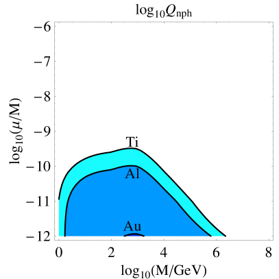
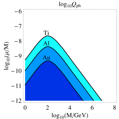
In order to achieve limits on the particle physics leading to $\mu-e$ conversion, the quark level effective Lagrangian of the model is adjusted to the form of Eq. (41) and by identifying the effective parameters $\eta_{AB}^{(q)}$ with expressions in terms of model parameters. This way the upper bounds on $Q_{a}$ from Table 2 can be translated to restrictions on the model parameters present in these expressions. Figure 3 shows the sensitivity bounds on the parameters $M$ and $\mu$ characterizing the inverse seesaw model, that follow from experiments with Al, Au and Ti targets, respectively.

It is also interesting to explore how these rates depend on the relevant neutrino mixing angles which are probed in solar neutrino experiments. This is shown in figure 4, where the relation between $R(\mu^{-}\text{Ti}\to e^{-}\text{Ti})$ ($Br(\mu\to e\gamma)$) and the solar neutrino angle $\theta_{12}$ for fixed $M$ and $\mu$ is displayed. As can be seen in the figure, there is also a strong dependence on the small neutrino mixing angle $\theta_{13}$.

In designing future experiments testing for $L_{f}/\hskip 5.0pt$ it is instructive to determine how the branching ratios for $\mu^{-}-e^{-}$ conversion and the $\mu^{-}\to e^{-}\gamma$ are related. In Fig. 5 we show explicitly that, in the inverse seesaw model, the rates for $\mu^{-}-e^{-}$ conversion and that for the $\mu^{-}\to e^{-}\gamma$ decay are strongly correlated, indicating the dominance of the photonic diagram in Fig. 1(a).

VI Summary and Conclusions

In the present paper we constructed an effective Lagrangian describing the photonic and non-photonic $\mu^{-}-e^{-}$ conversion in the context of the inverse seesaw model and specified the $L_{f}/\hskip 5.0pt$ parameters characterizing this process. We focused in the simplest inverse seesaw model. The interest in the model is that it accounts for the observed masses and mixings indicated by current oscillation data in such a way that the underlying physics “does not decouple” and can be phenomenologically probed experimentally. The model provides a framework for enhanced $L_{f}/\hskip 5.0pt$ rates with a rather simple, almost minimalistic, particle content. In contrast to the conventional seesaw, this is achieved without need of supersymmetrization. We derived a general formula for the coherent $\mu^{-}-e^{-}$ conversion branching ratio in terms of the $L_{f}/\hskip 5.0pt$ parameters of the above quark level effective Lagrangian and we calculated the corresponding nuclear matrix elements of currently interesting nuclear targets like ¹⁹⁷Au (the current SINDRUM II target), ²⁷Al (the target of the ongoing MECO experiment) and ⁴⁸Ti (the target for the upcoming PRISM experiment). These results are given in table 2 and can be used to obtain sensitivity limits from existing or planned experiments on $L_{f}/\hskip 5.0pt$ parameters in a variety of particle physics models. We have considered in detail the new important contributions to $\mu^{-}-e^{-}$ conversion present in the inverse seesaw model that come from the exchange of the relatively light SU(2) $\otimes$ U(1) singlet neutral leptons. Figure 3 shows the sensitivity bounds on the parameters $M$ and $\mu$ characterizing the inverse seesaw model, that follow from experiments with Al, Au and Ti, respectively. On the other hand figure 4 displays the relation of the $L_{f}/\hskip 5.0pt$ rates with the relevant neutrino mixing angles, while Fig. 5 establishes that, in the inverse seesaw model, the rates for $\mu^{-}-e^{-}$ conversion and that for the $\mu^{-}\to e^{-}\gamma$ decay are highly correlated.

This work was supported by Spanish grant BFM2002-00345, by the European Commission Human Potential Program RTN network MRTN-CT-2004-503369. T.S.K. and F.D. would like to express their appreciation to IFIC for hospitality.

Nucleus	$|{\bf p}_{e}|\,(fm^{-1})$	$\Gamma_{\mu c}\,(10^{6}\,s^{-1})$	${\cal M}^{2}_{ph}\,(fm^{-3})$	${\cal M}^{2}_{nph}\,(fm^{-3})$	${\quad\qquad\cal\phi\qquad\quad}$
12C	0.533	0.0388	0.00007	0.00029	0.0000
27Al	0.532	0.705	0.00204	0.00821	-0.0022
32S	0.531	1.352	0.00433	0.01656	0.0225
40Ca	0.529	2.557	0.00982	0.03667	0.0350
48Ti	0.528	2.590	0.01217	0.05560	-0.0645
63Cu	0.524	5.676	0.02883	0.12631	-0.0445
90Zr	0.517	8.660	0.06713	0.29713	-0.0493
112Cd	0.511	10.610	0.08416	0.37712	-0.0552
197Au	0.485	13.070	0.15571	0.68691	-0.0478
208Pb	0.482	13.450	0.18012	0.80892	-0.0563
238U	0.474	13.100	0.19360	0.87797	-0.0608

Table 1: Ingredients entering Eq. (61) which gives the branching ratio of the charged lepton flavour violating $\mu-e$ conversion for a set of nuclei throughout the periodic table. We note that by neglecting the electron mass we have $E_{e}\approx p_{e}c$.

Parameter	Present limits (PSI)	Expected limits (MECO)	Expected limits (PRISM)
	197Au	27Al	48Ti
${\cal Q}_{ph}$	$1.96\cdot 10^{-16}$	$2.68\cdot 10^{-18}$	$8.39\cdot 10^{-20}$
${\cal Q}_{nph}$	$4.45\cdot 10^{-15}$	$6.67\cdot 10^{-19}$	$1.84\cdot 10^{-20}$

Table 2: Upper bounds on the parameters $Q_{a}$ (see text, for definition) inferred from the SINDRUM II data on the $\mu^{-}-e^{-}$ conversion in ¹⁹⁷Au [Eq. (2)] as well as from the expected sensitivities of the current MECO (BNL) [Eq. (3)] and PRISM (KEK) experiments [Eq. (4)] with ²⁷Al and ⁴⁸Ti stopping targets respectively.

References

• (1) Super-Kamiokande collaboration, Y. Fukuda et al., Phys. Rev. Lett. 81, 1562 (1998), [hep-ex/9807003].
• (2) SNO collaboration, Q. R. Ahmad et al., Phys. Rev. Lett. 89, 011301 (2002), [nucl-ex/0204008].
• (3) KamLAND collaboration, K. Eguchi et al., Phys. Rev. Lett. 90, 021802 (2003), [hep-ex/0212021].
• (4) M. Maltoni, T. Schwetz, M. A. Tortola and J. W. F. Valle, New J. Phys. 6, 122 (2004), [hep-ph/0405172] and references therein
• (5) J. Hisano, T. Moroi, K. Tobe and M. Yamaguchi, Phys. Rev. D53, 2442 (1996), [hep-ph/9510309].
• (6) T. S. Kosmas, G. K. Leontaris and J. D. Vergados, Prog. Part. Nucl. Phys. 33, 397 (1994), [hep-ph/9312217].
• (7) T. S. Kosmas and J. D. Vergados, Nucl. Phys. A510, 641 (1990).
• (8) T. S. Kosmas, S. Kovalenko and I. Schmidt, Phys. Lett. B511, 203 (2001), [hep-ph/0102101].
• (9) T. S. Kosmas, Nucl. Phys. A683, 443 (2001).
• (10) A. Faessler, T. S. Kosmas, S. Kovalenko and J. D. Vergados, Nucl. Phys. B587, 25 (2000).
• (11) R. Kitano, M. Koike, S. Komine and Y. Okada, Phys. Lett. B575, 300 (2003), [hep-ph/0308021].
• (12) A. van der Schaaf, J. Phys. G29, 1503 (2003).
• (13) W. R. Molzon, Prepared for International Conference on Symmetries in High-Energy Physics and Applications, Ioannina, Greece, 30 Sep - 5 Oct 1998.
• (14) Y. Kuno, AIP Conf. Proc. 542, 220 (2000).
• (15) P. Minkowski, Phys. Lett. B67, 421 (1977); M. Gell-Mann, P. Ramond and R. Slansky, (1979), Print-80-0576 (CERN); T. Yanagida, (KEK lectures, 1979), ed. Sawada and Sugamoto (KEK, 1979); R. N. Mohapatra and G. Senjanovic, Phys. Rev. Lett. 44, 912 (1980); J. Schechter and J. W. F. Valle, Phys. Rev. D22, 2227 (1980); Phys. Rev. D25, 774 (1982); G. Lazarides, Q. Shafi and C. Wetterich, Nucl. Phys. B 181 (1981) 287.
• (16) R. N. Mohapatra and J. W. F. Valle, Phys. Rev. D34, 1642 (1986).
• (17) J. Bernabeu et al., Phys. Lett. B187, 303 (1987).
• (18) G. C. Branco, M. N. Rebelo and J. W. F. Valle, Phys. Lett. B225, 385 (1989). N. Rius and J. W. F. Valle, Phys. Lett. B246, 249 (1990).
• (19) F. Deppisch and J. W. F. Valle, Phys. Rev. D72, 036001 (2005), [hep-ph/0406040].
• (20) E. Akhmedov, M. Lindner, E. Schnapka and J. W. F. Valle, Phys. Rev. D53, 2752 (1996), [hep-ph/9509255]; Phys. Lett. B368, 270 (1996), [hep-ph/9507275].
• (21) S. M. Barr and I. Dorsner, hep-ph/0507067.
• (22) T. Fukuyama, A. Ilakovac, T. Kikuchi and K. Matsuda, JHEP 06, 016 (2005), [hep-ph/0503114].
• (23) M. Malinsky, J. C. Romao and J. W. F. Valle, Phys. Rev. Lett. 95, 161801 (2005), [hep-ph/0506296].
• (24) J. Schwieger, T. S. Kosmas and A. Faessler, Phys. Lett. B443, 7 (1998).
• (25) J. W. F. Valle, Phys. Rev. D27, 1672 (1983).
• (26) M. C. Gonzalez-Garcia and J. W. F. Valle, Phys. Lett. B216, 360 (1989).
• (27) Z. G. Berezhiani, A. Y. Smirnov and J. W. F. Valle, Phys. Lett. B291, 99 (1992), [hep-ph/9207209].
• (28) M. Dittmar et al., Nucl. Phys. B332, 1 (1990). M. C. Gonzalez-Garcia, A. Santamaria and J. W. F. Valle, Nucl. Phys. B342, 108 (1990).
• (29) DELPHI, P. Abreu et al., Z. Phys. C74, 57 (1997).
• (30) J. Schechter and J. W. F. Valle, Phys. Rev. D22, 2227 (1980)
• (31) J. A. Casas and A. Ibarra, Nucl. Phys. B618, 171 (2001), [hep-ph/0103065].
• (32) F. Deppisch, H. Paes, A. Redelbach, R. Ruckl and Y. Shimizu, Eur. Phys. J. C28, 365 (2003), [hep-ph/0206122].
• (33) F. Deppisch, H. Pas, A. Redelbach, R. Ruckl and Y. Shimizu, Phys. Rev. D69, 054014 (2004), [hep-ph/0310053].
• (34) N. Panagiotides and T. Kosmas, Artificial neural network techniques in solving Schroedinger and Dirac equations for tau and mu capture rates (Proc. MEDEX-03, in press, 2003).
• (35) R. Kitano, M. Koike and Y. Okada, Phys. Rev. D66, 096002 (2002), [hep-ph/0203110].
• (36) C. W. De Jager, H. De Vries and C. De Vries, Atom. Data Nucl. Data Tabl. 36, 495 (1987).
• (37) W. R. Gibbs and B. F. Gibson, Ann. Rev. Nucl. Part. Sci. 37, 411 (1987).
• (38) T. Suzuki, D. F. Measday and J. P. Roalsvig, Phys. Rev. C35, 2212 (1987).
• (39) A. Ilakovac and A. Pilaftsis, Nucl. Phys. B 437, 491 (1995) [arXiv:hep-ph/9403398].