Two- and Three-Particle Correlations in $q,\!p$-Bose Gas Model

Combined Analysis of Two- and Three-Particle
Correlations in $\boldsymbol{q,\!p}$-Bose Gas Model

Alexandre M. GAVRILIK A.M. Gavrilik

N.N. Bogolyubov Institute for Theoretical Physics, Kyiv, Ukraine omgavr@bitp.kiev.ua

Received December 29, 2005, in final form October 28, 2006; Published online November 07, 2006

$q$-deformed oscillators and the $q$-Bose gas model enable effective description of the observed non-Bose type behavior of the intercept (“strength”) $\lambda^{(2)}\equiv C^{(2)}(K,K)-1$ of two-particle correlation function $C^{(2)}(p_{1},p_{2})$ of identical pions produced in heavy-ion collisions. Three- and $n$-particle correlation functions of pions (or kaons) encode more information on the nature of the emitting sources in such experiments. And so, the $q$-Bose gas model was further developed: the intercepts of $n$-th order correlators of $q$-bosons and the $n$-particle correlation intercepts within the $q,\!p$-Bose gas model have been obtained, the result useful for quantum optics, too. Here we present the combined analysis of two- and three-pion correlation intercepts for the $q$-Bose gas model and its $q,\!p$-extension, and confront with empirical data (from CERN SPS and STAR/RHIC) on pion correlations. Similar to explicit dependence of $\lambda^{(2)}$ on mean momenta of particles (pions, kaons) found earlier, here we explore the peculiar behavior, versus mean momentum, of the 3-particle correlation intercept $\lambda^{(3)}(K)$. The whole approach implies complete chaoticity of sources, unlike other joint descriptions of two- and three-pion correlations using two phenomenological parameters (e.g., core-halo fraction plus partial coherence of sources).

$q$- and $q,\!p$-deformed oscillators; ideal gas of $q,\!p$-bosons; $n$-particle correlations; intercepts of two and three-pion correlators

81R50; 81V99; 82B99

1 Introduction

If, instead of treating particles as point-like structure-less objects, one attempts to take into account either nonzero proper volume or composite nature of particles, then it is natural to modify or deform [1, 2] the standard commutation relations. For these and many other reasons, so-called $q$-deformed oscillators play important role in modern physics, and various quantum or $q$-deformed algebras show their efficiency in diverse problems of quantum physics, see e.g. [3, 4, 5, 6, 7, 8, 9, 10, 11, 12]. In quantum optics, $q$-deformed oscillators and $q$-bosons enable more adequate modeling of the essentially nonlinear phenomena [6]. It is worth to mention the usage of both the quantum counterpart $U_{q}(su(n))$ of the Lie algebras of flavor groups $SU(n)$, and the algebras of $q$-deformed oscillators, in the context of phenomenology of hadron properties [7, 8, 9, 10, 11, 12].

As it was demonstrated recently, the approach first proposed in [13, 14] based on some set of $q$-deformed oscillators along with the related model of ideal gas of $q$-bosons is quite successful [15] if one attempts to effectively describe the observed, in experiments on relativistic heavy-ion collisions, non-Bose type properties of the intercept (“strength”) $\lambda^{(2)}\equiv C^{(2)}(p,p)-1$ of two-particle correlation function $C^{(2)}(p_{1},p_{2})$ of the pions emitted and registered in such experiments. Note that some other aspects related to this approach were developed in [16, 17].

Possible reasons for the intercept $\lambda^{(2)}$ to attain (not the expected Bose value $\lambda^{(2)}=1$, but) the values lesser than $1$ and thus the reasons to use such $q$-deformed structures as $q$-oscillators and the related model of ideal gas of $q$-bosons for an effective description, include:

1. finite proper volume of particles [1];

2. substructure of particles [1, 2];

3. memory effects;

4. effects from long-lived resonances (e.g., mimicked in the core-halo picture);

5. possible existence of non-chaotic (partially coherent) components of emitting sources;

6. non-Gaussian (effects of the) sources;

7. particle-particle, or particle-medium interactions (making pion gas non-ideal);

8. fireball is a short-lived, highly non-equilibrium and complicated system.

Clearly, items in this list may be interrelated, say, (a)–(b); (b)–(c); (e)–(f)–(h).

Three-particle correlation functions $C^{(3)}(p_{1},p_{2},p_{3})$ of identical pions (or kaons) are as well important, as those carry additional information [18, 19] on the space-time geometry and dynamics of the emitting sources; for the analysis of data, certain combination [18, 19] of two- and three-pion correlation functions is usually exploited in which the effects of long-lived resonances cancel out.

Further extension of main points of the approach based on $q$-Bose gas model has been done in [20]: (i) the intercepts of $n$-particle correlation functions have been obtained within $q$-Bose gas model in its two – Arik–Coon (AC) and Biedenharn–Macfarlane (BM) – main versions; (ii) closed expressions for the intercepts of $n$-particle correlation functions have been derived using two-parameter ($q,\!p$-) generalization of the deformed Bose gas model. The reason to employ the $q,\!p$-deformed Bose gas model is two-fold: first, the general formulae contain the AC and BM versions as particular cases; second, the $q,\!p$-Bose gas model provides a tools to take into account, in a unified way, any two independent reasons (to use $q$-deformation) from the above list.

Remark that the results in [20] are of general value: they can be utilized on an equal footing both in the domain of quantum optics if $n$-particle distributions and correlations are important, and in the analysis of multi-boson (-pion or -kaon) correlations in heavy ion collisions.

Our goal is to give, within the $q$-Bose gas model and its two-parameter extended $q,\!p$-Bose gas model, a unified analysis of two- and three-particle correlation functions intercepts using explicit formulas for $C^{(2)}(p,p)$, $C^{(3)}(p,p,p)$ [20] and a special combination $r^{(3)}(p,p,p)$ [18, 19] that involves both $C^{(2)}$ and $C^{(3)}$. Also, we pay some attention to a comparison of analytical results with the existing data on pion correlations from CERN SPS or STAR/RHIC experiments.

We emphasize a nontrivial shape of dependence on the mean momenta of pions (or kaons), not only for $C^{(2)}(p,p)$ found earlier but also for $C^{(3)}(p,p,p)$ and $r^{(3)}(p,p,p)$ studied here: the dependence turns out to be peculiar for both low and large mean momenta. The large momentum asymptotics is very special as it is determined by the deformation parameters $q,\!p$ only.

The whole our treatment assumes complete chaoticity of sources, in contrast to other approaches [21, 22, 23, 24] to simultaneous description of two- and three-pion correlations in terms of two phenomenological parameters where, in the core-halo picture, one of the parameters reflects partial non-chaoticity or coherence and the other means a measure of core fraction.

2 $\boldsymbol{q}$-oscillators and $\boldsymbol{q,\!p}$-oscillators

First, let us recall the well-known $q$-deformed oscillators of the Arik–Coon (AC) type [25, 26, 27],

$$a_{i}a_{j}^{\dagger}-q^{\delta_{ij}}a_{j}^{\dagger}a_{i}=\delta_{ij},\qquad[a_{i},a_{j}]=[a^{\dagger}_{i},a^{\dagger}_{j}]=0,$$ (1)

$$[{\cal N}_{i},a_{j}]=-\delta_{ij}a_{j},\qquad[{\cal N}_{i},a^{\dagger}_{j}]=\delta_{ij}a^{\dagger}_{j},\qquad[{\cal N}_{i},{\cal N}_{j}]=0,$$

viewed as a set of independent modes. Here and below, $-1\leq q\leq 1$. Basis state vectors $|n_{1},\ldots,n_{i},\ldots\rangle$ are constructed from vacuum state $|0,0,\ldots\rangle$ as usual, and the operators $a^{\dagger}_{i}$ act with matrix elements $\langle\ldots,n_{i}+1,\ldots|a^{\dagger}_{i}|\ldots,n_{i},\ldots\rangle=\sqrt{\lfloor n_{i}+1\rfloor}$ where the “basic numbers” $\lfloor r\rfloor\equiv{(1-q^{r})}/{(1-q)}$ are used. The $q$-bracket $\lfloor A\rfloor$ for an operator $A$ means formal series. As the $q$-parameter $q\to 1$, the $\lfloor r\rfloor$ resp. $\lfloor A\rfloor$ goes back to $r$ resp. $A$. The operators $a^{\dagger}_{i},$ $a_{i}$ are mutual conjugates if $-1\leq q\leq 1$. Note that the equality $a^{\dagger}_{i}a_{i}={\cal N}_{i}$ holds only at $q=1$, while for $q\neq 1$ the $a^{\dagger}_{i}a_{i}$ depends on the number operator ${\cal N}_{i}$ nonlinearly:

$$a^{\dagger}_{i}a_{i}=\lfloor{\cal N}_{i}\rfloor.$$ (2)

The system of the two-parameter extended or $q,\!p$-deformed oscillators is defined as [28]

$$A_{i}A_{j}^{\dagger}-q^{\delta_{ij}}A_{j}^{\dagger}A_{i}=\delta_{ij}p^{N_{i}^{(qp)}},\qquad A_{i}A_{j}^{\dagger}-p^{\delta_{ij}}A_{j}^{\dagger}A_{i}=\delta_{ij}q^{N_{i}^{(qp)}},$$ (3)

along with the relations $[N^{(qp)},A]=-A$, $[N^{(qp)},A^{\dagger}]=A^{\dagger}$. For the $q,\!p$-deformed oscillators,

$$A^{\dagger}A=[\![N^{(qp)}]\!]_{qp},\qquad[\![X]\!]_{qp}\equiv(q^{X}-p^{X})/(q-p).$$ (4)

At $p=1$ the AC-type $q$-bosons are recovered.

On the other hand, putting $p=q^{-1}$ in (3) yields the other important for our treatment case, the $q$-deformed oscillators of Biedenharn–Macfarlane (BM) type [29, 30] with the main relation

$$b_{i}b_{j}^{\dagger}-q^{\delta_{ij}}b_{j}^{\dagger}b_{i}=\delta_{ij}q^{-N_{j}}.$$ (5)

The ($q$-)deformed Fock space is constructed likewise, but now, instead of basic numbers, we use the other $q$-bracket and “$q$-numbers” (compare this with the brackets used in (2) and (4)):

$$b^{\dagger}_{i}b_{i}=[N_{i}]_{q},\qquad[r]_{q}\equiv(q^{r}-q^{-r})/(q-q^{-1}).$$ (6)

The equality $b^{\dagger}_{i}b_{i}=N_{i}$ holds only if $q=1$. For consistency of conjugation we put

$$q=\exp(i\theta),\qquad 0\leq\theta<\pi.$$ (7)

3 $\boldsymbol{q}$-deformed and $\boldsymbol{q,\!p}$-deformed momentum distributions

Dynamical multi-particle (multi-pion, -kaon, -photon, …) system will be viewed as an ideal gas of $q$- or $q,\!p$-bosons whose statistical properties are described by evaluating the thermal averages

$$\langle A\rangle=\frac{{\rm Sp}(Ae^{-\beta H})}{{\rm Sp}(e^{-\beta H})},\qquad H=\sum_{i}{\omega_{i}{\cal N}_{i}},\qquad\omega_{i}=\sqrt{m^{2}+{\boldsymbol{k}}_{i}^{2}},$$ (8)

where summation runs over different modes, $\beta=1/T$, and the Boltzmann constant is set $k=1$. In the Hamiltonian in (8), ${\cal N}_{i}$ denotes the number operator of the respective version: the AC-type, BM-type, or $q,\!p$-type. The $3$-momenta of particles are assumed to be discrete-valued.

The $q$-distribution for AC-type $q$-bosons ($-1\leq q\leq 1$) is $\langle a_{i}^{\dagger}a_{j}\rangle=\delta_{ij}\langle a_{i}^{\dagger}a_{i}\rangle=\delta_{ij}/(e^{\beta\omega_{i}}-q),$ reducing to the usual Bose–Einstein distribution if $q\to 1$. From now on, all the formulas will correspond to the mono-mode case (coinciding modes), and we shall omit the indices.

At $q=0$ or $q=-1$, the distribution function $\langle a^{\dagger}a\rangle=(e^{\beta\omega}-q)^{-1}$ yields the familiar classical Boltzmann or the Fermi–Dirac cases (the latter only formally: differing modes of $q$-bosons at $q=-1$ are commuting, unlike genuine fermions whose non-coinciding modes anticommute).

The one-particle momentum distribution function for the AC-type $q$-bosons, along with one-particle distributions for the BM-type $q$-bosons and for the general $q,\!p$-Bose gas case, are placed in the following Table 1 (first column). The second column of this same Table contains the two-particle mono-mode momentum distributions, correspondingly, for the three mentioned cases of deformed Bose gas. The results concerning one-particle distributions are known from the papers [31, 32, 33] whereas those on two-particle distributions from [13, 14, 34].

Table 1: One-particle and two-particle distributions of the ($q$- or $qp$-) deformed bosons.

Case	1-particle distribution	2-particle distribution
AC-case	$\langle a^{\dagger}a\rangle=\frac{1}{e^{\beta\omega}-q}$	$\langle{a^{\dagger}}^{2}a^{2}\rangle=\frac{(1+q)}{(e^{\beta\omega}-q)(e^{\beta\omega}-q^{2})}$
BM-case	$\langle b^{\dagger}b\rangle=\frac{e^{\beta\omega}-1}{e^{2\beta\omega}-(q+q^{-1})e^{\beta\omega}+1}$	$\langle{b^{\dagger}}^{2}b^{2}\rangle=\frac{(q+q^{-1})}{(e^{\beta\omega}-q^{2})(e^{\beta\omega}-q^{-2})}$
$q,\!p$-bosons	$\langle A^{\dagger}A\rangle=\frac{(e^{\beta\omega}-1)}{(e^{\beta\omega}-p)(e^{\beta\omega}-q)}$	$\langle{A^{\dagger}}^{2}A^{2}\rangle=\frac{(p+q)(e^{\beta\omega}-1)}{(e^{\beta\omega}-q^{2})(e^{\beta\omega}-pq)(e^{\beta\omega}-p^{2})}$

Few remarks are in order. (i) The $q$-distribution functions for the AC case (first row) are real for real deformation parameter $q$. The $q$-distribution functions for the BM case (second row) are real not only with real deformation parameter, but also for $q=\exp(i\theta)$, in which case we have: $q+q^{-1}=[2]_{q}=2\cos\theta$, and $q^{2}+q^{-2}=[2]_{q^{2}}=2\cos(2\theta)$. The $q,\!p$-distributions, see third row, are real if both $q$ and $p$ are real, or $|q|=1$ and $p=q^{-1}$, or $p=\bar{q}$. (ii) Each of the two one-particle $q$-deformed distributions (AC-type or BM-type $f_{q}({\boldsymbol{k}})\equiv\langle b^{\dagger}b\rangle({\boldsymbol{k}})$) is such that at $q\neq 1$ the corresponding curve is intermediate between the familiar Bose–Einstein and Boltzmann curves. (iii) Generalized $q,\!p$-deformed one- and two-particle distribution functions given in third row, reduce to the corresponding distributions of the $q$-bosons of AC-type in the first row if $p=1$ (BM type in the second row if $p=q^{-1}$). (iv) Here and below, all the two-parameter $q,\!p$-expressions possess the interchange symmetry under $q\leftrightarrow p$.

4 $\boldsymbol{n}$-particle distributions and correlations of deformed bosons

The most general result, derived in [20] and based on the $q,\!p$-oscillators, for the $n$-particle distribution functions of the gas of $q,\!p$-bosons

$$\langle{A^{\dagger}}^{n}A^{n}\rangle=\frac{[\![n]\!]_{qp}!\ (e^{\beta\omega}-1)}{\prod\limits_{r=o}^{n}(e^{\beta\omega}-q^{r}p^{n-r})},\qquad[\![m]\!]_{qp}!=[\![1]\!]_{qp}[\![2]\!]_{qp}\cdots[\![m-1]\!]_{qp}[\![m]\!]_{qp},$$ (9)

involves the $q,\!p$-bracket defined in (4). Let us remark that this general formula for the $n$-th order, or $n$-particle, mono-mode momentum distribution functions for the ideal gas of $q,\!p$-bosons follows from combining the following two relations

$$\langle A^{{\dagger}n}A^{n}\rangle=\frac{[\![n]\!]_{qp}!}{\prod_{r=0}^{n-1}(e^{\beta\omega}-p^{r}q^{n-r})}{\langle p^{nN}\rangle}\qquad{\rm and}\qquad{\langle p^{nN}\rangle}=\frac{e^{\beta\omega}-1}{e^{\beta\omega}-p^{n}}.$$ (10)

Below, we are interested in the $q,\!p$-deformed intercept $\lambda^{(n)}_{q,p}\equiv-1+\frac{{\langle A^{\dagger n}A^{n}\rangle}}{{\langle A^{\dagger}A\rangle}^{n}}$ of $n$-particle correlation function. The corresponding formula constitutes main result in [20] and reads:

$$\lambda^{(n)}_{q,p}=[\![n]\!]_{qp}!\frac{(e^{\beta\omega}-p)^{n}(e^{\beta\omega}-q)^{n}}{(e^{\beta\omega}-1)^{n-1}\prod\limits_{k=0}^{n}(e^{\beta\omega}-q^{n-k}p^{k})}-1.$$ (11)

Consider the asymptotics $\beta\omega\to\infty$ (for large momenta or, with fixed momentum, for low temperature) of the intercepts $\lambda^{(n)}_{q,p}$:

$$\lambda^{(n),\,{\rm asym.}}_{q,p}=-1+[\![n]\!]_{qp}!=-1+\prod^{n-1}_{k=1}\biggl{(}\sum^{k}_{r=0}q^{r}p^{k-r}\biggl{)}.$$ (12)

It is worth noting that for each case: the $q$-bosons of AC-type, of BM-type, and the $q\!p$-bosons, the asymptotics of $n$-th order intercept is given by the corresponding deformed extension of $n$-factorial (the intercept of pure Bose–Einstein $n$-particle correlator is given by the usual $n!$).

To specialize these results for particular case of AC-type $q$-bosons we set $p=1$. The $n$-particle distribution function and the $n$-th order intercept $\lambda^{(n)}\equiv\frac{\langle a^{\dagger n}a^{n}\rangle}{\langle a^{\dagger}a\rangle^{n}}-1$ take the form

$$\langle{a^{\dagger}}^{n}a^{n}\rangle=\frac{\lfloor n\rfloor!}{\prod\limits_{r=1}^{n}(e^{\beta\omega}-q^{r})},\qquad\lambda^{(n)}_{\rm{AC}}=-1+\frac{\lfloor n\rfloor!\ (e^{\beta\omega}-q)^{n-1}}{\prod\limits^{n}_{r=2}(e^{\beta\omega}-q^{r})},$$ (13)

where $\lfloor m\rfloor\equiv\frac{1-q^{m}}{1-q}=1+q+q^{2}+\dots+q^{m-1}$. At $\beta\omega\to\infty$ the result involves only $q$-parameter:

$$\lambda^{(n),\,{\rm asym.}}_{\rm{AC}}=-1+\lfloor n\rfloor!=-1+\prod^{n-1}_{k=1}\biggl{(}\sum^{k}_{r=0}q^{r}\biggr{)}$$

$$\phantom{\lambda^{(n),\,{\rm asym.}}_{\rm{AC}}}{}=(1+q)(1+q+q^{2})\cdots(1+q+\cdots+q^{n-1})-1.$$

This constitutes a principal consequence of the approach. It would be very nice to verify this, using the data for pions and kaons drawn from the experiments on relativistic nuclear collisions.

The expressions for the BM case that are parallel to (13) follow from the general formulas (9), (11), (12) if we put $p=q^{-1}$.

Intercepts of two- and three-particle correlation functions, their asymptotics. Let us consider the 2nd and 3rd order correlation intercepts. In Table 2 we present the intercepts of two-particle correlations for the $q$-bosons of AC-type and BM-type, as well as for the general case of $q,\!p$-bosons. Recall that at $p=q^{-1}$, $[\![2]\!]_{qp}\equiv p+q$ reduces to $[2]_{q}=q+q^{-1}=2\cos\theta$.

Table 2: Intercept of two-particle correlations of deformed bosons and its asymptotics.

Case	Intercept $\lambda^{(2)}\equiv\frac{\langle a^{\dagger 2}a^{2}\rangle}{\langle a^{\dagger}a\rangle^{2}}-1$	Asymptotics of $\lambda^{(2)}$ at $\beta\omega\to\infty$
AC	$\lambda^{(2)}_{\rm AC}=\frac{(1+q)(e^{\beta\omega}-q)}{e^{\beta\omega}-q^{2}}-1=q\frac{e^{\beta\omega}-1}{e^{\beta\omega}-q^{2}}$	$\lambda^{(2),\,{\rm asym.}}_{\rm AC}=q$
BM	$\lambda^{(2)}_{\rm BM}=\frac{2\cos\theta(e^{2\beta\omega}-2\cos\theta\ e^{\beta\omega}+1)^{2}}{(e^{\beta\omega}-1)^{2}(e^{2\beta\omega}-2\cos(2\theta)e^{\beta\omega}+1)}-1$	$\lambda^{(2),\,{\rm asym.}}_{\rm BM}=2\cos\theta-1$
$q,\!p$	$\lambda^{(2)}_{q,p}=\frac{(p+q)(e^{\beta\omega}-p)^{2}(e^{\beta\omega}-q)^{2}}{(e^{\beta\omega}-1)(e^{\beta\omega}-q^{2})(e^{\beta\omega}-pq)(e^{\beta\omega}-p^{2})}-1$	$\lambda^{(2),\,{\rm asym.}}_{q,p}=(p+q)-1$

In the non-deformed limit $q\to 1$ (or $\theta\to 0$) the value $\lambda_{\rm BE}=1$ known for Bose–Einstein statistics is correctly reproduced from the formulas in the first two rows of Table 2. This obviously corresponds to the Bose–Einstein distribution recovered from the $q$-Bose one at $q\to 1$. Now consider three-particle correlations. The intercepts for all the three versions of deformed Bose gas along with their asymptotics are presented in Table 3 as three rows correspondingly. We end with two remarks valid for both the Table 2 and Table 3. First, the formulas for AC- or BM-type follow from those of the $q,\!p$-Bose gas (given in the third row) if we set $p=1$ or $p=q^{-1}$. Second, as demonstrated by the last column, the large $\beta\omega$ asymptotics of each of the three versions of $\lambda^{(3)}$ is given by a very simple dependence on the deformation parameter(s) only.

Table 3: Intercepts of three-particle correlations of deformed bosons and their asymptotics.

Case	Intercept $\lambda^{(3)}\equiv\frac{\langle a^{\dagger 3}a^{3}\rangle}{\langle a^{\dagger}a\rangle^{3}}-1$	Asymptotics of $\lambda^{(3)}$ at $\beta\omega\to\infty$
AC	$\lambda^{(3)}_{\rm AC}=\frac{(1+q)(1+q+q^{2})(e^{\beta\omega}-q)^{2}}{(e^{\beta\omega}-q^{2})(e^{\beta\omega}-q^{3})}-1$	$\lambda^{(3),\,{\rm asym.}}_{\rm AC}=(1+q)(1+q+q^{2})-1\!\!$
BM	$\lambda^{(3)}_{\rm BM}=\frac{2\cos\!\theta(4\cos^{2}\theta-1)(e^{2\beta\omega}-2\cos\!\theta\ e^{\beta\omega}+1)^{2}}{(e^{\beta\omega}-1)^{2}(e^{2\beta\omega}-2\cos(3\theta)e^{\beta\omega}+1)}-1$	$\lambda^{(3),\,{\rm asym.}}_{\rm BM}=2\cos\theta(4\cos^{2}\theta-1)-1\!\!$
$q,\!p$	$\lambda^{(3)}_{q,p}\!=\!\frac{(p+q)(p^{2}+pq+q^{2})(e^{\beta\omega}-p)^{3}(e^{\beta\omega}-q)^{3}}{(e^{\beta\omega}-1)^{2}(e^{\beta\omega}-p^{3})(e^{\beta\omega}-p^{2}q)(e^{\beta\omega}-pq^{2})(e^{\beta\omega}-q^{3})}\!-\!1\!\!$	$\lambda^{(3),\,{\rm asym.}}_{q,p}\!=\!(p+q)(p^{2}+pq+q^{2})\!-\!1\!\!$

5 Comparison with data on two- and three-pion correlations

The explicit dependence, via $\beta\omega=\frac{1}{T}\sqrt{m^{2}+K_{\rm t}^{2}}$, of the intercept $\lambda^{(2)}_{\rm BM}$ on transverse mean momentum is shown in Fig. 1 where the empirical values on negative pions [35, 36], for three momentum bins (horizontal bars), are shown as the crosses. At $T\!=\!180$ MeV, these three values agree perfectly with the curve E for which $q=\exp(i\theta)$, $\theta=28.5^{\circ}$. Slightly higher temperature $T=205$ MeV gives nice agreement of empirical values with the curve of $\theta=\frac{\pi}{7}\simeq 25.7^{\circ}$, twice the Cabibbo angle. We may conjecture that, this way, the hot pions in their correlations show some “memory” of their origin as quark-antiquark bound states, see the items (b)–(c) in Introduction. Possible relation of the Cabibbo (quark mixing) angle to the value $q$ of deformation which measures deviation of the $q$-Bose gas picture from pure Bose one, looks quite promising. However, more empirical data for two-pion (-kaon) correlations with more bins for diverse momenta in experiments on relativistic nuclear collisions are needed in order to confirm within this model the general trend and the key feature that for $\beta\omega\to\infty$ (large momenta, or low temperatures) the intercept does saturate with a value given by deformation parameter(s) only.

Equally good comparison of the data for two-particle correlations of positive pions [35, 36] with the AC-type of $q$-Bose gas model at the optimal $q=0.63$ was achieved [15], and general observation was made that the AC-type $q$-Bose gas model with real $q$ is well suited for treating $\pi^{+}\pi^{+}$ correlations, while the BM version with $q=e^{i\theta}$ serves better for $\pi^{-}\pi^{-}$ correlations.

Figure 1: Intercept $\lambda^{(2)}_{\rm BM}$ versus pions’ transverse momentum $K_{\rm t}$, at $T=180$ MeV and $q=\exp(i\theta)$: A) $\theta=6^{\circ}$; B) $\theta=10^{\circ}$; C) $\theta=22^{\circ}$; D) $\theta=25.7^{\circ}$, i.e. $2\theta_{c}$; E) $\theta=28.5^{\circ}$. The $\pi^{-}\pi^{-}$ data are taken from [35, 36].

In Fig. 2 we plot the dependence on particles’ mean momentum for the 3rd order correlation intercept $\lambda_{\rm BM}^{(3)}$ of the BM version of $q$-Bose gas. Observe the asymptotic saturation with constant values fixed by $q$ (or $\theta$), as Table 3 prescribes. Also, a peculiar behavior of the intercept $\lambda_{\rm BM}^{(3)}$ is evident: at low momenta it acquires zero or even negative values for some curves, see “E”, “F”. However, these two curves imply large angles $\theta$ (large deviations from pure Bose value $\theta=0$), the cases hardly realizable in view of the items (a)-(h) of Introduction. Curves similar to those in Fig. 2 can be presented for the 3rd order intercept $\lambda_{\rm AC}^{(3)}$ of the AC-type of $q$-Bose gas model.

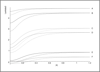
Figure 2: Intercept $\lambda_{\rm BM}^{(3)}$  versus pions’ mean momentum $|{\bf K}|$, GeV/c. The temperature is 120 MeV (180 MeV) for solid (dashed) curves. In each pair the two curves have common asymptotics given, see Table 3, by the value of $\theta$, from the top down: $\frac{\pi}{30}$ (A); $\frac{\pi}{14}$ (B); $\frac{\pi}{7}$ (C); $\frac{28.5\pi}{180}$ (D); $\frac{9.26\pi}{40}$ (E); $\frac{\pi}{4}$ (F).

Now compare the explicit form of the intercepts $\lambda^{(2)}_{p,q}$ and $\lambda^{(3)}_{p,q}$ of two- and three-particle correlations of $p,\!q$-bosons from Tables 2, 3 with the available data on the 2nd and 3rd order correlations of pions [35, 36, 37, 38] from the experiments on relativistic nuclear collisions, namely [37, 38]

$$\lambda^{(2),{\rm exp.}}|_{\rm neg.pions}=0.57\pm 0.04,$$ (14)

$$\lambda^{(3),{\rm exp.}}|_{\rm neg.pions}=1.92\pm 0.49.$$ (15)

Equating the expression for say $\lambda^{(2)}_{p,q}(w)$ from Table 2 (with $w\equiv\beta\omega$) to some fixed value, in particular those in (14), (15), leads to an implicit function $w=w(q,\!p)$ whose image is 2-surface. Fig. 3 (left) shows the two surfaces obtained from equating $\lambda^{(2)}_{p,q}$ resp. $\lambda^{(3)}_{p,q}$ to the central values of the data $\lambda^{(2),{\rm exp}}$ resp. $\lambda^{(3),{\rm exp}}$ in (14), (15). As seen, these “central” surfaces are very close to each other, for both low and large values of $w$ (recall, $w\equiv\beta\omega=T^{-1}\sqrt{m^{2}+K_{\rm t}^{2}}$); only in their lower right corner the surfaces are seen as disjoint. For comparison, in Fig. 3 (right) we show the result of equating $\lambda^{(2)}_{p,q}(w)$ resp. $\lambda^{(3)}_{p,q}(w)$ to the upper value $\lambda^{(2),{\rm exp.}}_{+}=0.57+0.04$ resp. lower value $\lambda^{(3),{\rm exp.}}_{-}=1.92-0.49$ in (14), (15). Here the resulting two surfaces are clearly distant. Likewise, using the values $\lambda^{(2),{\rm exp.}}_{-}=0.57\!-\!0.04$, $\lambda^{(3),{\rm exp.}}_{+}=1.92+0.49$ in (14), (15), we get yet another two surfaces which we do not exhibit. In total, due to (14), (15) we have six surfaces: the three (named “$\lambda^{(2)}$-triple”) obtained by equating $\lambda^{(2)}_{p,q}(w)$ to each of the 3 values $\lambda^{(2),{\rm exp.}}$ in (14), and the other three (named “$\lambda^{(3)}$-triple”) got by equating $\lambda^{(3)}_{p,q}(w)$ to each value in (15).

Cutting the both triples of surfaces by a horizontal plane $w=w_{0}$ with some fixed $w_{0}$ yields, in this plane, six curves given as six implicit functions $q=q(p)$. In Fig. 4, we exhibit the result of slicing these two triples by $w=0.78$ (left panel), and by $w=2.9$ (right panel). In each panel we observe that (the strip formed by) $\lambda^{(3)}$-triple of curves fully covers (the strip of) $\lambda^{(2)}$-triple. Such full covering differs from the situation in [21, 22, 23, 24] where only the imaging of data with 2$\sigma$ (or 3$\sigma$) uncertainty gave some overlapping. Also unlike [21, 22, 23, 24], we present explicit momentum dependence for $\lambda^{(2)}$, $\lambda^{(3)}$. Besides, our approach assumes complete chaoticity of particle sources.

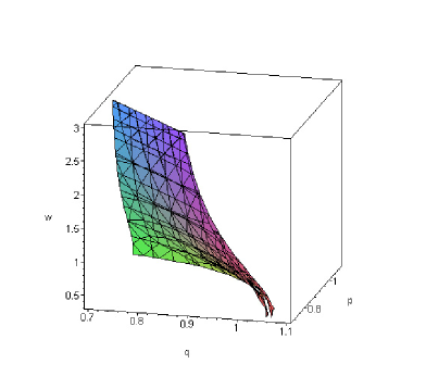
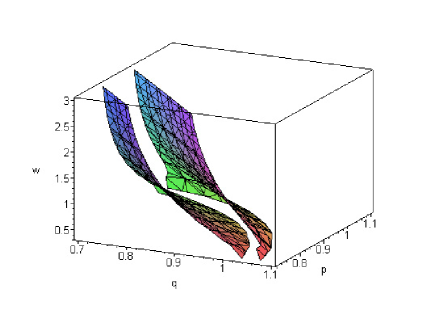
Figure 3: Left: The two “central” surfaces as implicit functions $w=w(q,\!p)$: one stems from equating $\lambda^{(2)}_{p,q}(w)$ from Table 2 to the central value $\lambda^{(2),{\rm exp.}}=0.57$ in (14), the other stems from equating $\lambda^{(3)}_{p,q}(w)$ from Table 3 to the central value $\lambda^{(3),{\rm exp.}}=1.92$ in (15). Notice mutual closeness of these “central” surfaces. Right: similar to the left panel, but now $\lambda^{(2)}_{p,q}(w)$ is equated to $\lambda^{(2),{\rm exp.}}_{+}=0.57+0.04$ in (14) and $\lambda^{(3)}_{p,q}(w)$ to $\lambda^{(3),{\rm exp.}}_{-}=1.92-0.49$ in (15).

  

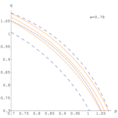
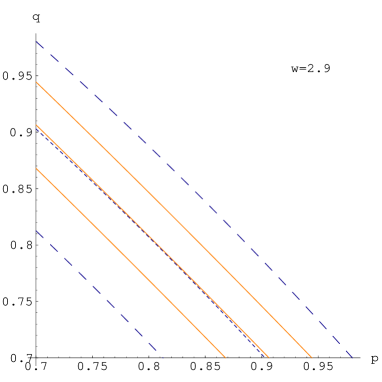
Figure 4: Left: Slice of all the six surfaces (two pairs in Fig. 3 and the remaining 2 surfaces, see main text) by putting $w=0.78$. Solid (dashed) lines stem from cutting the $\lambda^{(2)}$-triple (the $\lambda^{(3)}$-triple) of surfaces. Right: same as left panel, but now $w=2.9$ is put. Notice full overlapping of $\lambda^{(2)}$-strip and $\lambda^{(3)}$-strip.

Let us make few remarks concerning Figs. 3 and 4.

1) The two very near “central” surfaces of Fig. 3 (left) reflect themselves in Fig. 4 as follows: the result of their slicing by $w=0.78$ is seen in the left panel as the two very close lines, one solid and one dashed, which connect the points given roughly as (1.05, 0) and (0, 1.05), while the result of their slicing by $w=2.9$ is seen in the right panel as the two almost straight, almost coinciding solid and dashed lines given roughly by the equation $q=0.9-p$. On the other hand, the two distant surfaces of Fig. 3 (right) yield after their slicing the lowest dashed and the uppermost solid lines in each panel of Fig. 4.

2) In both left and right panels of Fig. 4, the entire strip formed by the three solid (i.e., $\lambda^{(2)}$-) curves, lies completely within the strip formed by the three dashed $\lambda^{(3)}$-curves. The larger width of the latter strip is due to better accuracy of data in (14) as compared with that in (15).

3) Limiting ourselves to one-parameter cases, from Figs. 3, 4 we deduce: beside the AC-type ($p=1$) and BM-type ($p=q^{-1}$) $q$-oscillators defined in (1) and (5) and their versions of $q$-Bose gas, there is yet another distinguished case of $q$-oscillator and so yet another version of $q$-Bose gas model equally well suited for explaining the experimental data: this is the $q$-oscillator which is contained in the relations (3), (4) at $p=q$ and which also leads, by applying $p=q$, to the corresponding formulas for distributions, intercepts etc. for this version of $q$-Bose gas.

4) It is easily seen from Fig. 4 that the TD-type of $q$-Bose gas model constructed on the base of the TD-type $q$-oscillator (see footnote 4) is more preferable than the AC version for description of the data like (14) and (15): first, it needs narrower range of values of the $q$-parameter in order to cover the data (14), (15) including the uncertainties; second, with just these data the use of AC version is problematic for the large momenta region because of $p=1$, see right panel of Fig. 4, while on the contrary the TD version corresponding to $p=q$ serves equally well for both small ($w=0.78$) and large ($w=2.9$) values of momenta.

Unified analysis of $\lambda^{(2)}$ and $\lambda^{(3)}$ versus empirical data using special combination. For a unified analysis of data on the two- and three-particle correlations, there exists [18, 19] a very convenient special combination designed in terms of correlators, namely

$$r^{(3)}(p_{1},p_{2},p_{3})\equiv\frac{1}{2}\frac{C^{(3)}(p_{1},p_{2},p_{3})-C^{(2)}(p_{1},p_{2})-C^{(2)}(p_{2},p_{3})-C^{(2)}(p_{3},p_{1})+2}{\sqrt{\left(C^{(2)}(p_{1},p_{2})-1\right)\left(C^{(2)}(p_{2},p_{3})-1\right)\left(C^{(2)}(p_{3},p_{1})-1\right)}},$$

which with the restriction $p_{1}=p_{2}=p_{3}=K$ turns into the simple expression

$$r^{(3)}_{j}(K)\equiv r^{(3)}_{j}(K,K,K)=\frac{1}{2}\frac{\lambda_{j}^{(3)}(K)-3\lambda_{j}^{(2)}(K)}{\bigl{(}\lambda_{j}^{(2)}(K)\bigr{)}^{3/2}}$$ (16)

composed of just the intercepts. Here $\lambda^{(2)}(K)=C^{(2)}(K,K)-1$, $\lambda^{(3)}(K)=C^{(3)}(K,K,K)-1$, and the subscript $j$ denotes the particular type (AC, BM, TD, or $q,\!p$-) of the deformed Bose gas. The relevant formulas for the intercepts involved are to be taken from Tables 2, 3. The convenience of (16) from the viewpoint of comparison with data is two-fold: first, the design of $r^{(3)}$ is such that the contribution to it from long-lived resonances cancels out [18, 19]; second, the $r^{(3)}$ carries an additional meaning being a (cosine of) special phase [42].

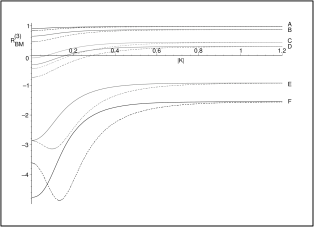
Figure 5: Plot of $r^{(3)}_{\rm BM}({\bf K})$ from (16) with the intercepts $\lambda^{(2)}_{\rm BM}$, $\lambda^{(3)}_{\rm BM}$, versus pions’ mean momentum $|{\bf K}|$, GeV/c. For solid (dashed) lines $T=120$ MeV ($T=180$ MeV). In each pair, the two curves have common asymptotics determined by its $\theta$ value: $\frac{\pi}{30}$ (A), $\frac{\pi}{14}$ (B), $\frac{\pi}{7}$ (C), $\frac{28.5\pi}{180}$ (D), $\frac{9.26\pi}{40}$ (E), $\frac{\pi}{4}$ (F).

In Fig. 5, taking as example the one-parameter BM version of $q$-Bose gas model, we show main features of the momentum dependence of $r_{\rm BM}^{(3)}({\bf K})$. Again the behavior is rather peculiar as it shows nontrivial shape in the small $|{\bf K}|$ region, asymptotic saturation with a constant determined by $q$ (or $\theta$) at large $|{\bf K}|$, and the property that the value of temperature $T$ is very important. Of course, it will be very interesting to check the validity of such a behavior by confronting with relevant empirical data. We only note that the presently available data on the $r^{(3)}$ values [35, 36] are controversial (the set of values ranges from zero to unity) and insufficient, usually not indicating to which momenta bins they correspond.

6 Conclusions and outlook

We have demonstrated the efficiency of the generalized $q,\!p$-deformed Bose gas model in combined description of the intercepts of two- and three-particle correlations, especially in view of the non-Bose type properties of the 2nd and 3rd order correlations of pions (and kaons) observed in the experiments on relativistic collisions of heavy nuclei. The key advantages of the model are: (i) it provides the explicit dependence on particle’s mean momentum of the intercepts $\lambda^{(2)}$, $\lambda^{(3)}$ as well as of their combination $r^{(3)}$ given in (16); (ii) it possesses the asymptotical property that at $\beta\omega\to\infty$ each of these quantities becomes independent of particles’ mass, momentum and temperature and takes a very simple form determined by the deformation parameters $q,\!p$ only. The property (ii) is important as it enables, using the empirical data on $\lambda^{(2)}$ and $\lambda^{(3)}$ for sufficiently large transverse momenta, to determine with high accuracy the values of the deformation parameters $q,p$ which, in accord with our paradigm, should characterize the nontrivial and special system under study, see the items (a)–(h) of Introduction. With so fixed deformation parameters and due to (i), one should use the low transverse momentum data for $\lambda^{(2)}$ and $\lambda^{(3)}$ in order to firmly fix the value of temperature.

A remark on the one-parameter limiting cases of the $q,\!p$-Bose gas model. From the Figs. 3, 4 we have deduced that, beside the most popular BM- and AC-cases of $q$-Bose gas model, yet another distinguished one-parameter case is of interest: this is the Tamm–Dancoff (TD) version of $q$-deformed oscillators and $q$-Bose gas model, got from the general two-parameter $q,\!p$-formulas by putting $p=q$. The TD case provides as well an appropriate basis for the analysis of data on two-, three- and possibly multi-particle momentum correlators (first of all, correlation intercepts) of pions and kaons from the experiments like those reported in [35, 36, 37, 38].

We have seen from the Figs. 1, 3, 4, that the $q,\!p$-Bose gas model, which is an extension of the $q$-Bose gas model, is in agreement with presently available experimental data. Concerning the data from experiments [35, 36] especially those on the intercept of 3-pion correlations and the quantity $r^{(3)}$, it is highly desirable to obtain not only the values averaged over large range of transverse mean momenta or transverse mass of identical particles, but also a more detailed data with numerous momentum bins, for both small and large transverse momenta. A rich enough set of momentum-attributed values of $\lambda^{(3)}$ and $r^{(3)}$ will allow to draw more certain conclusions about the viability of the considered model. With detailed experimental data, further judgements will be possible about actual physical meaning (recall the items (a)–(h) in the Introduction) and adequate values of the deformation parameter(s) $q$ or $q,\!p$. This includes the special one-parameter case of the BM-type $q$-Bose gas model with its possible link [11, 12] of the $q$-parameter $\ q=\exp(i\theta)$ to the Cabibbo (quark mixing) angle.

Of course, more work is needed to further develop the approach based on the concept of $q,\!p$-Bose gas. Note that in our study of the implications of the $q,\!p$-Bose gas model and subsequent analysis of relevant data, we dealt only with the intercept (i.e. the strength) of the two-pion as well as three- and multi-pion correlation functions. Put in another words, we treated only the mono-mode (single-mode) case which means coinciding momenta of the correlated particles. Since within general $q,\!p$-deformation of Bose gas model it is desirable to have a complete correlation functions with full momentum dependence including nonzero relative momenta of particles, clearly the multi-mode case should be elaborated. Although the modeling of complete correlation functions is highly non-unique (see e.g. [43]) and not too trivial, as a first step one may proceed in analogy to the one parameter $q$-Bose gas model (e.g. like in [16]).

Acknowledgements

The author is grateful to Professor R. Jagannathan for sending a copy of his paper. This work is partially supported by the Grant 10.01/015 of the State Foundation of Fundamental Research of Ukraine.

References

- [1] Avancini S.S., Krein G., Many-body problems with composite particles and -Heisenberg algebras, J. Phys. A: Math. Gen., 1995, V.28, 685–691.
- [2] Perkins W.A., Quasibosons, Internat. J. Theoret. Phys., 2002, V.41, 823–838, hep-th/0107003.
- [3] Chang Z., Quantum group and quantum symmetry, Phys. Rep., 1995, V.262, 137–225, hep-th/9508170.
- [4] Kibler M.R., Introduction to quantum algebras, hep-th/9409012.
- [5] Mishra A.K., Rajasekaran G., Generalized Fock spaces, new forms of quantum statistics and their algebras, Pramana, 1995, V.45, 91–139, hep-th/9605204.
- [6] Man’ko V.I., Marmo G., Sudarshan E.C.G., Zaccaria F., -oscillators and nonlinear coherent states, Phys. Scripta, 1997, V.55, 528–541, quant-ph/9612006.
- [7] Gavrilik A.M., -Serre relations in , -deformed meson mass sum rules, and Alexander polynomials, J. Phys. A: Math. Gen., 1994, V.27, L91–L94.
- [8] Gavrilik A.M., Iorgov N.Z., Quantum groups as flavor symmetries: account of nonpolynomial -breaking effects in baryon masses, Ukrain. J. Phys., 1998, V.43, 1526–1533, hep-ph/9807559.
- [9] Chaichian M., Gomez J.F., Kulish P., Operator formalism of q deformed dual string model, Phys. Lett. B, 1993, V.311, 93–97, hep-th/9211029.
- [10] Jenkovszky L., Kibler M., Mishchenko A., Two-parametric quantum deformed dual amplitude, Modern Phys. Lett. B, 1995, V.10, 51–60, hep-ph/9407071.
- [11] Gavrilik A.M., Quantum algebras in phenomenological description of particle properties, Nucl. Phys. B (Proc. Suppl.), 2001, V.102, 298–305, hep-ph/0103325.
- [12] Gavrilik A.M., Quantum groups and Cabibbo mixing, in Proceedings of Fifth International Conference “Symmetry in Nonlinear Mathematical Physics” (June 23–29, 2003, Kyiv), Editors A.G. Nikitin, V.M. Boyko, R.O. Popovych and I.A. Yehorchenko, Proceedings of Institute of Mathematics, Kyiv, 2004, V.50, Part 2, 759–766, hep-ph/0401086.
- [13] Anchishkin D.V., Gavrilik A.M., Iorgov N.Z., Two-particle correlations from the -Boson viewpoint, Eur. Phys. J. A, 2000, V.7, 229–238, nucl-th/9906034.
- [14] Anchishkin D.V., Gavrilik A.M., Iorgov N.Z., -Boson approach to multiparticle correlations, Modern Phys. Lett. A, 2000, V.15, 1637–1646, hep-ph/0010019.
- [15] Anchishkin D.V., Gavrilik A.M., Panitkin S., Intercept parameter of two-pion (-kaon) correlation functions in the -boson model: character of its -dependence, Ukrain. J. Phys., 2004, V.49, 935–939, hep-ph/0112262.
- [16] Zhang Q.H., Padula S.S., -boson interferometry and generalized Wigner function, Phys. Rev. C, 2004, V.69, 24907, 11 pages, nucl-th/0211057.
- [17] Gutierrez T., Intensity interferometry with anyons, Phys. Rev. A, 2004, V.69, 063614, 5 pages, quant-ph/0308046.
- [18] Wiedemann U.A., Heinz U., Particle interferometry for relativistic heavy-ion collisions, Phys. Rept., 1999, V.319, 145–230, nucl-th/9901094.
- [19] Heinz U., Zhang Q.H., What can we learn from three-pion interferometry? Phys. Rev. C1997, V.56, 426–431, nucl-th/9701023.
- [20] Adamska L.V., Gavrilik A.M., Multi-particle correlations in -Bose gas model, J. Phys. A: Math. Gen., 2004, V.37, N 17, 4787–4795, hep-ph/0312390.
- [21] Csorgö T. et al., Partial coherence in the core/halo picture of Bose–Einstein -particle correlations, Eur. Phys. J. C, 1999, V.9, 275–281, hep-ph/9812422.
- [22] Csanad M. for PHENIX Collab., Measurement and analysis of two- and three-particle correlations, nucl-ex/0509042.
- [23] Morita K., Muroya S., Nakamura H., Source chaoticity from two- and three-pion correlations in Au+Au collisions at GeV, nucl-th/0310057.
- [24] Biyajima M., Kaneyama M., Mizoguchi T., Analyses of two- and three-pion Bose–Einstein correlations using Coulomb wave functions, Phys. Lett. B, 2004, V.601, 41–50, nucl-th/0312083.
- [25] Arik M., Coon D.D., Hilbert spaces of analytic functions and generalized coherent states, J. Math. Phys., 1976, V.17, 524–527.
- [26] Fairlie D., Zachos C., Multiparameter associative generalizations of canonical commutation relations and quantized planes, Phys. Lett. B, 1991, V.256, 43–49.
- [27] Meljanac S., Perica A., Generalized quon statistics, Modern Phys. Lett. A, 1994, V.9, 3293–3300.
- [28] Chakrabarti A., Jagannathan R., A ()oscillator realization of two-parameter quantum algebras, J. Phys. A: Math. Gen., 1991, V.24, L711–L718.
- [29] Macfarlane A.J., On -analogues of the quantum harmonic oscillator and the quantum group , J. Phys. A: Math. Gen., 1989, V.22, 4581–4585.
- [30] Biedenharn L.C., The quantum group and a -analogue of the boson operators, J. Phys. A: Math. Gen., 1989, V.22, L873–L878.
- [31] Altherr T., Grandou T., Thermal field theory and infinite statistics, Nucl. Phys. B, 1993, V.402, 195–216.
- [32] Vokos S., Zachos C., Thermodynamic -distributions that aren’t, Modern Phys. Lett. A, 1994, V.9, 1–9.
- [33] Lavagno A., Narayana Swamy P., Thermostatistics of deformed boson gas, Phys. Rev. E, 2000, V.61, 1218–1226, quant-ph/9912111.
- [34] Daoud M., Kibler M., Statistical mechanics of -bosons in dimensions, Phys. Lett. A, 1995, V.206, 13–17, quant-ph/9512006.
- [35] Adler C. et al. [STAR Collab.], Pion interferometry of = 130-GeV Au+Au collisions at RHIC, Phys. Rev. Lett., 2001, V.87, 082301, 6 pages, nucl-ex/0107008.
- [36] Adams J. et al. [STAR Collab.], Three-pion HBT correlations in relativistic heavy-ion collisions from the STAR experiment, Phys. Rev. Lett., 2003, V.91, 262301, 6 pages, nucl-ex/0306028.
- [37] Aggarwal M.M. et al. [WA98 Collab.], One-, two- and three-particle distributions from 158 GeV/ central Pb+Pb collisions, Phys. Rev. C, 2003, V.67, 014906, 24 pages, nucl-ex/0210002.
- [38] Bearden I.G. et al. [NA44 Collab.], One-dimensional and two-dimensional analysis of 3 pi correlations measured in Pb + Pb interactions, Phys. Lett. B, 2001, V.517, 25–31, nucl-ex/0102013.
- [39] Cheng T.-P., Li L.-F., Gauge theory of elementary particle physics, Oxford, Clarendon Press, 1984.
- [40] Odaka K., Kishi T., Kamefuchi S., On quantization of simple harmonic oscillators, J. Phys. A: Math. Gen., 1991, V.24, L591–L596.
- [41] Chaturvedi S., Srinivasan V., Jagannathan R., Tamm–Dancoff deformation of bosonic oscillator algebras, Modern Phys. Lett. A, 1993, V.8, 3727–3734.
- [42] Heiselberg H., Vischer A.P., The phase in three-pion correlations, nucl-th/9707036.
- [43] Csorgo T., Szerzo A.T., Model independent shape analysis of correlations in 1, 2 or 3 dimensions, Phys. Lett. B, 2000, V.489, 15–23, hep-ph/0011320.