Rare decays of $B\to J/\psi D^{(*)}$ and $B\to\eta_{c}D^{(*)}$ in pQCD Approach

Abstract

Motivated by the recent measurement of the upper limit of ${B}^{0}\to J/\psi D$ branching ratio, which is important in accounting for the soft $J/\psi$ production in $B$ decays, we investigate ${B}^{0}\to J/\psi D^{(\star)}$ and $\eta_{c}D^{(\star)}$ decays in perturbative QCD approach based on $k_{T}$ factorization. Being pure annihilation (W-exchange) decays, these branching ratios are estimated to be at the order of $10^{-5}\sim 10^{-7}$, which are just at the corner of being observable at the $B$ factories. The measurements of these decay channels may help us to understand the QCD dynamics in the corresponding energy scale, especially the reliability of pQCD approach to these processes.

I Introducrion

In 1995, the CLEO Collaboration found a hump in the low momentum region of the inclusive spectrum of $B\to J/\psi+X$ decay Cleo . Later on, this observation was confirmed by Belle Belle and BaBar Babar . In these measurements, there is an excess in the momentum spectrum of the $J/\psi$ recoiling mass at $\sim 2~{}\mathrm{GeV}$. And, the excess corresponds to a branching ratio of $6\times 10^{-4}$. In order to explain this result, various hypotheses have been proposed brod ; hou ; yang .

In Ref. hou , Chang and Hou employ the idea of intrinsic charm Incharm $c\bar{c}$ inside the $B$ meson to this issue. Based on this scenario, they predicted that the branching ratio of $B\to J/\psi D$ should be about $10^{-4}$. However, according to recent BaBar and Belle measurements, the branching ratio upper limit of this process is less than $10^{-5}$ ep1 ; ep2 , which implies that the intrinsic charm mechanism is not favored. In another scenario, in which the charmonium is produced predominantly in the Color-Octet mechanism, Eilam and Yang estimated the branching ratio of $B\to J/\psi D$ yang and got a result of about $10^{-8}$. However, in the collinear factorization, they have to use a cut-off or $\delta$-function to tame the end-point singularity. Hence, their numerical results are not stable. The recent progress in perturbative QCD (pQCD) treatment, based on the $k_{T}$ factorization, of $B$ meson decays can solve this problem by introducing the Sudakov form factor through the threshold resummation. Now, the pQCD approach LY has become one of the broadly used theoretical methods in investigating the $B$ meson two-body non-leptonic decays. Base on the pQCD approach, many $B$ meson decay modes have been calculated, like $B\to K\pi,\pi\pi$ hep-ph/9411308 , etc., and most results are consistent with the experimental data. Since there is no end-point singularity, the pQCD approach can also be applied to the pure ”annihilation processes ”, such as $B\to D_{s}K$ bdsk .

In this work, we calculate the $B\to J/\psi D^{(*)}$ and $B\to\eta_{c}D^{(*)}$ processes in the pQCD $k_{T}$ factorization. In the decay of $B\to J/\psi D$, the $W$ boson exchange induces the four quark operator $\bar{c}b\to\bar{u}d$, and an additional pair of $c\bar{c}$ is created by a gluon. This gluon can attach to any quark involving in the four-quark operator. In the rest frame of $B$ meson, the produced $c$ and $\bar{c}$ quarks in the final states have the momenta of order $\mathcal{O}(P_{\psi}/2)$ and $\mathcal{O}(P_{D}/2)$, respectively. Therefore, the gluon, which generates the charm quark pair, possesses a virtuality of order $\sim\mathcal{O}(M_{B}/2)$, which enables the perturbative QCD calculation reliable.

The paper is organized as follows: we present the formalism used in the calculation of $B\to J/\psi D^{(*)}$ and $B\to\eta_{c}D^{(*)}$ decays in Section II. In Section III we give out the numerical calculation results and some discussion on them. The last section is left for conclusions and summary.

II Kinematics

The effective Hamiltonian for decay modes $B\to J/\psi D^{(*)}$ and $B\to\eta_{c}D^{(*)}$ is given by Buchalla:1995vs

$${\cal H}_{\rm eff} = \frac{G_{F}}{\sqrt{2}}V_{cb}V_{ud}^{*}\left[C_{1}(\mu)O_{2}+C_{2}(\mu)O_{2}\right],$$ (1)

$$O_{1} = \bar{c}\gamma_{\mu}(1-\gamma_{5})u\,\bar{d}\gamma^{\mu}(1-\gamma_{5})b,$$

$$O_{2} = \bar{d}\gamma_{\mu}(1-\gamma_{5})u\,\bar{c}\gamma^{\mu}(1-\gamma_{5})b.$$ (2)

As usual, in the pQCD approach the momenta of the final states are expressed in its light-cone components, like

$$p=(p^{+},p^{-},\vec{p}_{T})=\left(\frac{p^{0}+p^{3}}{\sqrt{2}},\frac{p^{0}-p^{3}}{\sqrt{2}},(p^{1},p^{2})\right).$$ (3)

And, the decay amplitude can be generally written as:

$$\mathcal{M} \sim \int\!\!dx_{1}dx_{2}dx_{3}b_{1}db_{1}b_{2}db_{2}b_{3}db_{3}\$$ (4)

$$\times\mathrm{Tr}\bigl{[}C(t)\Phi_{B}(x_{1},b_{1})\Phi_{\psi}(x_{2},b_{2})\Phi_{D}(x_{3},b_{3})H(x_{i},b_{i},t)e^{-S(t)}\bigr{]}\;.$$

Here, $\mathrm{Tr}$ denotes the trace over Dirac and color indices. $C(t)$ is Wilson coefficient of the four quark operator which results from the radiative corrections at short distance. $\Phi_{M}$ denote the wave functions which are process independent and represent the non-perturbative dynamics of hadronization. The hard interaction kernel $H$ is, nevertheless, process-dependent and can be calculated by perturbation QCD. $t$ is chosen as the largest energy scale involving in the hard interaction to avoid the largest logarithms. $S(t)$ is Sudakov form factor resulted from the resummation of double logarithms hep-ph/9411308 ; hep-ph/9607214 . Therefore, in eq.(4) only the hard part is process dependent and will be calculated in the following.

II.1 The $B\to J/\psi D$ Decays

Of the $B$- and $D^{(*)}$-meson wavefunctions, we make use of the same parameterizations as used in the studies of different processes hep-ph/9411308 ; 0305335 . For vector $J/\psi$ meson, in terms of the notation in Ref. TLS , we decompose the nonlocal matrix elements for the longitudinally and transversely polarized $J/\psi$ mesons into

$$\langle J/\psi(P,\epsilon_{L})|\bar{c}(z)_{j}c(0)_{l}|0\rangle = \frac{1}{\sqrt{2N_{c}}}\int_{0}^{1}dxe^{ixP\cdot z}\bigg{\{}m_{J/\psi}[\not{\!\epsilon}_{L}]_{lj}\Psi^{L}(x)+[\not{\!\epsilon}_{L}\not{\!P}]_{lj}\Psi^{t}(x)\bigg{\}}\;,$$ (5)

$$\langle J/\psi(P,\epsilon_{T})|\bar{c}(z)_{j}c(0)_{l}|0\rangle = \frac{1}{\sqrt{2N_{c}}}\int_{0}^{1}dxe^{ixP\cdot z}\bigg{\{}m_{J/\psi}[\not{\!\epsilon}_{T}]_{lj}\Psi^{V}(x)+[\not{\!\epsilon}_{T}\not{\!P}]_{lj}\Psi^{T}(x)\bigg{\}}\;,$$ (6)

respectively. Here, $\Psi^{L}$ and $\Psi^{T}$ denote for the twist-2 distribution amplitudes, and $\Psi^{t}$ and $\Psi^{V}$ for the twist-3 distribution amplitudes. $x$ represents the momentum fraction of the charm quark inside the charmonium.

The $J/\psi$ meson asymptotic distribution amplitudes read as BC04

$$\Psi^{L}(x) = \Psi^{T}(x)=9.58\frac{f_{J/\psi}}{2\sqrt{2N_{c}}}x(1-x)\left[\frac{x(1-x)}{1-2.8x(1-x)}\right]^{0.7}\;,$$

$$\Psi^{t}(x) = 10.94\frac{f_{J/\psi}}{2\sqrt{2N_{c}}}(1-2x)^{2}\left[\frac{x(1-x)}{1-2.8x(1-x)}\right]^{0.7}\;,$$

$$\Psi^{V}(x) = 1.67\frac{f_{J/\psi}}{2\sqrt{2N_{c}}}\left[1+(2x-1)^{2}\right]\left[\frac{x(1-x)}{1-2.8x(1-x)}\right]^{0.7}\;,$$ (7)

in which the twist-3 ones $\Psi^{t,V}$ vanish, as the twist-2 ones, at the end points due to the factor $[x(1-x)]^{0.7}$. In contrast to Ref.yang , here we distinguish the longitudinal and transverse distribution amplitudes of the polarized $J/\psi$, which can exhibit the different asymptotic behaviors of these two types.

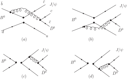
Figure 1: Feynman diagrams for ${B}^{0}\to J/\Psi\bar{D}^{0}$ decay process in pQCD.

From the effective Hamiltonian (1), the Feynman diagrams corresponding to the concerned process are drawn in Fig.1, where the heavy dots denote the four quark operators. Similar figures can be obtained by replacing the $J/\psi$ by $\eta_{c}$ for $B\to\eta_{c}D$ process, and $D$ by $D^{*}$ for the vector $D$-meson processes. With the meson wave functions and Sudakov factors, the hard amplitude for factorizable annihilation diagrams Figs.1(a) and (b) is

$$F_{a}=16\pi C_{F}M_{B}^{2}\int_{0}^{1}\!\!dx_{2}dx_{3}\int_{0}^{\infty}\!\!b_{2}db_{2}\,b_{3}db_{3}\ \phi_{D}(x_{3})\\ \times\Bigl{[}(x_{3}-1-x_{3}r_{3}^{2}-x_{3}r_{2}^{2})\Psi^{L}(x_{2})E_{f}(t_{1})h_{1}(x_{2},x_{3},b_{2},b_{3})-\bigl{\{}[x_{2}-1+\\ (1-2x_{2})r_{3}^{2}+(1-x_{2})r_{2}^{2}]\Psi^{L}(x_{2})+2x_{2}r_{2}r_{3}\Psi^{t}(x_{2})\bigr{\}}E_{f}(t_{2})h_{2}(x_{2},x_{3},b_{2},b_{3})\Bigr{]}.$$ (8)

Here, the functions $E_{f}(t_{a})$ contain Sudakov factors and Wilson coefficients of four quark operator, and hard scale $t_{a}$. The $h_{a}$, the virtual quark and gluon propagator, are given in the appendix.

The result for the non-factorizable annihilation processes, shown in Figs. 1(c) and (d), is

$$M_{a}=\frac{1}{\sqrt{2N_{c}}}64\pi C_{F}M_{B}^{2}\int_{0}^{1}\!\!dx_{1}dx_{2}dx_{3}\int_{0}^{\infty}\!\!b_{1}db_{1}\,b_{2}db_{2}\ \phi_{B}(x_{1},b_{1})\phi_{D}(x_{3})\\ \times\Bigl{[}\bigl{\{}(1-2r_{2}^{2})\left(1-x_{3}\right)\Psi^{L}(x_{2})+r_{2}\left(x_{2}-x_{3}\right)r_{3}\Psi^{t}(x_{2})\bigr{\}}E_{m}(t_{3})h_{3}(x_{1},x_{2},x_{3},b_{1},b_{2})\\ -\bigl{\{}(1-x_{2}-(1-2x_{2})r_{2}^{2}-(1-2x_{2}+x_{3})r_{3}^{2})\Psi^{L}(x_{2})\\ -r_{2}(x_{2}-x_{3})r_{3}\Psi^{t}(x_{2})\bigr{\}}E_{m}(t_{4})h_{4}(x_{1},x_{2},x_{3},b_{1},b_{2})\Bigr{]}.$$ (9)

The total decay amplitude for this decay is:

$${\cal A}_{a}(B\to J/\psi D)=f_{B}F_{a}+M_{a}.$$ (10)

Thus, the $B$ meson decay width of the concerned process is:

$$\Gamma(B\to J/\psi D)=\frac{G_{F}^{2}M_{B}^{3}}{128\pi}(1-r_{2}^{2}-r_{3}^{2})\left|{V_{cb}V_{ud}^{*}\cal A}_{a}(B\to J/\psi D)\right|^{2}.$$ (11)

II.2 The $B\to\eta_{c}D^{(*)}$ Decays

The nonlocal matrix element of $\eta_{c}$ production from vacuum can be generally expressed as

$$\langle\eta_{c}(P)|\bar{c}(z)_{j}c(0)_{l}|0\rangle = \frac{1}{\sqrt{2N_{c}}}\int_{0}^{1}dxe^{ixP\cdot z}\bigg{\{}[\gamma_{5}\not{\!P}]_{lj}\eta^{v}(x)+m_{\eta_{c}}[\gamma_{5}]_{lj}\eta^{s}(x)\bigg{\}}\;.$$ (12)

Here, $\eta^{v}(x)$ and $\eta^{s}(x)$ denote the twist-2 and twist-3 $\eta_{c}$ meson distribution amplitudes, respectively. The asymptotic forms of the $\eta_{c}$ distribution amplitudes are given in BC04 :

$$\eta^{v}(x) = 9.58\frac{f_{\eta_{c}}}{2\sqrt{2N_{c}}}x(1-x)\left[\frac{x(1-x)}{1-2.8x(1-x)}\right]^{0.7}\;,$$

$$\eta^{s}(x) = 1.97\frac{f_{\eta_{c}}}{2\sqrt{2N_{c}}}\left[\frac{x(1-x)}{1-2.8x(1-x)}\right]^{0.7}.$$ (13)

Performing the similar procedure as in above subsection, we can get the decay amplitudes for $B\to\eta_{c}D$ and $B\to\eta_{c}D^{*}$ straightforwardly.

II.3 The $B\to J/\psi D^{*}$ Decays

The $B\to J/\psi D^{*}$ decay rate are

$$\Gamma=\frac{G_{F}^{2}P_{c}}{32\pi M^{2}_{B}}\sum_{\sigma=L,T}{\cal A}^{(\sigma)\dagger}{\cal A^{(\sigma)}}\;,$$ (14)

where $P_{c}\equiv|P_{2z}|=|P_{3z}|$ are the momenta of the outgoing vector mesons; the superscript $\sigma$ denotes for the helicity states of the two vector mesons, the $L$ for the longitudinal and $T$ for the transverse components. The amplitude $\cal M^{(\sigma)}$ can be decomposed, according to the Lorentz structure, to hep-ph/9810475 :

$${\cal A}^{(\sigma)} = \epsilon_{2\mu}^{*}(\sigma)\epsilon_{3\nu}^{*}(\sigma)\left[a\,\,g^{\mu\nu}+{b\over m_{\Psi}m_{D}}P_{1}^{\mu}P_{1}^{\nu}+i{c\over m_{\Psi}m_{D}}\epsilon^{\mu\nu\alpha\beta}P_{2\alpha}P_{3\beta}\right]\;,$$ (15)

$$\equiv M_{B}^{2}{\cal A}_{L}+M_{B}^{2}{\cal A}_{N}\epsilon^{*}_{2}(\sigma=T)\cdot\epsilon^{*}_{3}(\sigma=T)+i{\cal A}_{T}\epsilon^{\alpha\beta\gamma\rho}\epsilon^{*}_{2\alpha}(\sigma)\epsilon^{*}_{3\beta}(\sigma)P_{2\gamma}P_{3\rho}\;,$$

with the convention $\epsilon^{0123}=1$ for the total anti-symmetric tensor and definitions

$$M_{B}^{2}\,\,{\cal A}_{L} = a\,\,\epsilon_{2}^{*}(L)\cdot\epsilon_{3}^{*}(L)+{b\over m_{\Psi}m_{D}}\epsilon_{2}^{*}(L)\cdot P_{1}\,\,\epsilon_{3}^{*}(L)\cdot P_{1}\;,$$

$$M_{B}^{2}\,\,{\cal A}_{N} = a\,\,\epsilon_{2}^{*}(T)\cdot\epsilon_{3}^{*}(T)\;,$$ (16)

$${\cal A}_{T} = {c\over m_{\Psi}m_{D}}\;.$$

Hereby, the only work left is to calculate the matrix elements $A_{L}$, $A_{N}$ and $A_{T}$ with

$$A_{i}=f_{B}F_{i}+M_{i},(i=L,N,T).$$ (17)

Here, $F_{i}$ and $M_{i}$, coming from the calculation of hard interaction, are given as follows:

$$F_{L}=16\pi C_{F}M_{B}^{2}\int_{0}^{1}\!\!dx_{2}dx_{3}\int_{0}^{\infty}\!\!b_{2}db_{2}\,b_{3}db_{3}\ \phi_{D}(x_{3})\\ \times\Bigl{[}(x_{3}-1-(x_{3}-2)r_{3}^{2}-(2x_{3}-1)r_{2}^{2})\Psi^{L}(x_{2})E_{f}(t_{1})h_{1}(x_{2},x_{3},b_{2},b_{3})\\ +\bigl{\{}[x_{2}-1+(1-2x_{2})r_{3}^{2}+(1-x_{2})r_{2}^{2}]\Psi^{L}(x_{2})\bigr{\}}E_{f}(t_{2})h_{2}(x_{2},x_{3},b_{2},b_{3})\Bigr{]},$$ (18)

$$F_{N}=16\pi C_{F}M_{B}^{2}\int_{0}^{1}\!\!dx_{2}dx_{3}r_{2}r_{3}\int_{0}^{\infty}\!\!b_{2}db_{2}\,b_{3}db_{3}\ \phi_{D}(x_{3})r_{2}r_{3}\\ \times\Bigl{[}(1-x_{3})\Psi^{V}(x_{2})E_{f}(t_{1})h_{1}(x_{2},x_{3},b_{2},b_{3})+\bigl{\{}(x_{2}-2)\Psi^{V}(x_{2})\bigr{\}}E_{f}(t_{2})h_{2}(x_{2},x_{3},b_{2},b_{3})\Bigr{]},$$ (19)

$$F_{T}=32\pi C_{F}M_{B}^{2}\int_{0}^{1}\!\!dx_{2}dx_{3}r_{2}r_{3}\int_{0}^{\infty}\!\!b_{2}db_{2}\,b_{3}db_{3}\ \phi_{D}(x_{3})r_{2}r_{3}\\ \times\Bigl{[}(1+x_{3})\Psi^{V}(x_{2})E_{f}(t_{1})h_{1}(x_{2},x_{3},b_{2},b_{3})+x_{2}\Psi^{V}(x_{2})E_{f}(t_{2})h_{2}(x_{2},x_{3},b_{2},b_{3})\Bigr{]},$$ (20)

$$M_{L}=\frac{1}{\sqrt{2N_{c}}}64\pi C_{F}M_{B}^{2}\int_{0}^{1}\!\!dx_{1}dx_{2}dx_{3}\int_{0}^{\infty}\!\!b_{1}db_{1}\,b_{2}db_{2}\ \phi_{B}(x_{1},b_{1})\phi_{D}(x_{3})\\ \times\Bigl{[}\bigl{\{}\left(x_{3}-1-2(x_{3}-1)(r_{3}^{2}+r_{2}^{2})\right)\Psi^{L}(x_{2})+r_{2}\left(x_{2}+x_{3}-2\right)r_{3}\Psi^{t}(x_{2})\bigr{\}}\\ \times E_{m}(t_{3})h_{3}(x_{1},x_{2},x_{3},b_{1},b_{2})+\bigl{\{}(1-x_{2}-(1-2x_{2})r_{2}^{2}-(1-2x_{2}-x_{3})r_{3}^{2})\Psi^{L}(x_{2})\\ -r_{2}(x_{2}+x_{3})r_{3}\Psi^{t}(x_{2})\bigr{\}}E_{m}(t_{4})h_{4}(x_{1},x_{2},x_{3},b_{1},b_{2})\Bigr{]},$$ (21)

$$M_{N}=\frac{1}{\sqrt{2N_{c}}}64\pi C_{F}M_{B}^{2}\int_{0}^{1}\!\!dx_{1}dx_{2}dx_{3}\int_{0}^{\infty}\!\!b_{1}db_{1}\,b_{2}db_{2}\ \phi_{B}(x_{1},b_{1})\phi_{D}(x_{3})\\ \times\Bigl{[}\bigl{\{}\left(x_{3}-1\right)r_{3}^{2}\Psi^{T}(x_{2})+\left(x_{2}-1\right)r_{2}^{2}\Psi^{T}(x_{2})\bigr{\}}E_{m}(t_{3})h_{3}(x_{1},x_{2},x_{3},b_{1},b_{2})\\ +\bigl{\{}(-x_{3}r_{3}^{2}\Psi^{T}(x_{2})+2r_{2}r_{3}\Psi^{V}(x_{2})-x_{2}r^{2}_{2}\Psi^{T}(x_{2})\bigr{\}}E_{m}(t_{4})h_{4}(x_{1},x_{2},x_{3},b_{1},b_{2})\Bigr{]},$$ (22)

$$M_{T}=\frac{1}{\sqrt{2N_{c}}}128\pi C_{F}M_{B}^{2}\int_{0}^{1}\!\!dx_{1}dx_{2}dx_{3}\int_{0}^{\infty}\!\!b_{1}db_{1}\,b_{2}db_{2}\ \phi_{B}(x_{1},b_{1})\phi_{D}(x_{3})\\ \times\Bigl{[}\bigl{\{}\left(x_{3}-1\right)r_{3}^{2}\Psi^{T}(x_{2})-\left(x_{2}-1\right)r_{2}^{2}\Psi^{T}(x_{2})\bigr{\}}E_{m}(t_{3})h_{3}(x_{1},x_{2},x_{3},b_{1},b_{2})\\ +\bigl{\{}(-x_{3}r_{3}^{2}\Psi^{T}(x_{2})+x_{2}r^{2}_{2}\Psi^{T}(x_{2})\bigr{\}}E_{m}(t_{4})h_{4}(x_{1},x_{2},x_{3},b_{1},b_{2})\Bigr{]}.$$ (23)

III Numerical Results

In this work, the input parameters for the numerical calculation are pdg , which are commonly used in literature,

$$m_{J/\psi}=3.097~{}\mathrm{GeV},m_{\eta_{c}}=2.980~{}\mathrm{GeV},f_{D^{*}}=230~{}\mathrm{MeV},$$

$$f_{D}=240~{}\mathrm{MeV},m_{D}=1.87~{}\mathrm{GeV},m_{D^{*}}=2.005~{}\mathrm{GeV},$$

$$m_{B}=5.28~{}\mathrm{GeV},|V_{cb}|=0.043,|V_{ud}|=0.975,\tau_{B}=1.54\times 10^{-12}~{}\mathrm{s}.$$ (24)

At leading order, the main uncertainty comes from the meson wave functions. Fortunately, the meson wave function, that describes hadronic process, is universal at a certain scale. For instance, the $B$ meson wave function is constrained by the measured exclusive hadronic decays, like $B\to\pi\pi,K\pi$hep-ph/9411308 with parameter $\omega_{B}$ from $0.32$ to $0.48$. To determine the $D$ meson wave function is more tough task than that of $B$ meson, because the heavy quark limit here is not as good as in the $B$ meson case. Referring to to $B\to D^{(*)}M$0305335 process, we can fit the $D$ meson wave function parameter to be $a_{D}=0.8\pm 0.2$. The charmonium distribution amplitudes can be inferred from the non-relativistic heavy quarkonium bound state wave functions, which have been shown to be successful in describing the charmonium production in $e^{+}e^{-}$ collisionsBC04 . The meson decay constant can be measured via its pure leptonic decay. We have $f_{J/\psi}=405\pm 14~{}\mathrm{MeV}$ and $f_{\eta_{c}}=420\pm 50~{}\mathrm{MeV}$. In addition to the uncertainties remaining in the above input parameters, the higher order corrections to the hard part are also important, which is discussed in Ref. hsiangnan .

Considering of the above uncertainties discussed, we can give out the branching ratios of the discussed processes with error bars:

$${\rm Br}({B}^{0}\to J/\psi D) = (3.45^{+1.22}_{-1.46}\pm 1.51\pm 0.32)\times 10^{-6},$$

$${\rm Br}({B}^{0}\to\eta_{c}D) = (1.28^{+0.32}_{-0.41}\pm 0.58\pm 0.35)\times 10^{-5},$$

$${\rm Br}({B}^{0}\to\eta_{c}D^{*}) = (8.26^{+2.82}_{-2.34}\pm 2.23\pm 2.06)\times 10^{-6},$$

$${\rm Br}({B}^{0}\to J/\psi D^{*}) = (7.04^{+2.43}_{-2.54}\pm 2.72\pm 0.53)\times 10^{-7}.$$ (25)

In the above, the uncertainties mainly come from $\omega_{B}$, $a_{D}$, and the decay constants, respectively. To diminish the uncertainties, for $B^{0}\to J/\psi D^{*}$ process, we evaluate the longitudinal polarization fraction, that is:

$$P_{L}=\frac{\Gamma_{L}}{\Gamma}=0.66.$$ (26)

This polarization fraction is not sensitive to the above mentioned input parameters, because they only give an equally change of each polarization amplitudes. However, this fraction is still sensitive to the $J/\psi$ wave function. If we set the distribution amplitude of transversal part the same as longitudinal part, the branching ratio become larger and the polarization fractions changed:

$${\rm Br}({B}^{0}\to J/\psi D^{*})=10.5\times 10^{-7}.$$ (27)

$$P_{L}=\frac{\Gamma_{L}}{\Gamma}=0.40;~{}~{}~{}P_{N,T}=\frac{\Gamma_{N,T}}{\Gamma}=0.30.$$ (28)

That is to say that for ${B}^{0}\to J/\psi D^{*}$ the most important uncertainty comes from the vector meson wave functions.

Compared to Ref. yang , our results are much bigger. In yang , all wave functions, which describe the non-perturbative hadronization, are $\delta$-function-like. However, the $\delta$-like wave function can not embody the relativistic corrections, though it can be used to avoid the end-point singularity due to the wave function overlap absent. In this work, the hadron distribution amplitudes are obtained from from the established models with experimental fittings. In our work, we take into account the Sudakov form factor and the transverse momentum $k_{T}$ distribution, which are unique characters of pQCD approach. For $B^{0}\to J/\psi D^{*}$ process, since the charmonium longitudinal distribution amplitude is different from its transverse one, and hence our longitudinal polarization fraction are larger than what obtained in Ref. yang .

Since there is only one kind of CKM phase involving in the concerned process, there should be no CP violation in these process within the standard model. On experimental side, so far there is only an upper limit for the branching ratio of ${B}^{0}\to J/\psi D$ process. That is

$${\rm Br}({B}^{0}\to J/\psi D) < 1.3\times 10^{-5}~{}~{}[8],$$

$${\rm Br}({B}^{0}\to J/\psi D) < 2.0\times 10^{-5}~{}~{}[9],$$ (29)

from different experiment group, which is larger than, but very close to our prediction.

IV Summary

In this work, we have calculated the decays of ${B}^{0}\to J/\psi(\eta_{c})D^{(*)}$ in the pQCD approach. These $B$ meson exclusive decay processes are in pure annihilation type, which is hard to be accurately calculated in other approaches with the end-point singularity. By keeping the transverse momentum $k_{T}$, the end-point singularity disappears in our calculation. Our numerical results shows that the branching ratios of ${B}^{0}\to\eta_{c}D$, ${B}^{0}\to\eta_{c}D^{*}$, ${B}^{0}\to J/\psi D$ and ${B}^{0}\to J/\psi D^{(*)}$ decay processes are of the order $10^{-5}$, $10^{-6}$, $10^{-6}$, and $10^{-7}$, respectively, which is just close to the experiment capability to measure them. Although both Belle and BaBar measured the $J/\psi$ momentum spectrum in $B$ inclusive decays, they did not obtain the branching ratios of these exclusive decays modes. Considering that the upper limits set by experiments are very close to our predictions. We suggest that BaBar and Belle measure these exclusive processes in near future. The observation of these exclusive processes may greatly improve our understanding on the $B$ meson exclusive hadronic decays, and the corresponding theory describing them as well.

Appendix A Some functions

The function $E_{f}^{i}$, $E_{m}$, and $E^{\prime}_{m}$ including Wilson coefficients are defined as

$$E_{f}(t)=(C_{1}(t)+\frac{C_{2}(t)}{N_{c}})\alpha_{s}(t)\,e^{-S_{\Psi}(t)-S_{D}(t)},$$ (30)

$$E_{m}(t)=C_{2}(t)\alpha_{s}(t)\,e^{-S_{B}(t)-S_{\Psi}(t)-S_{D}(t)}.$$ (31)

where $S_{B}$, $S_{\Psi}$, and $S_{D}$ result from summing both double logarithms caused by soft gluon corrections and single ones due to the renormalization of ultra-violet divergence. The above $S_{B,\Psi,D}$ are defined as

$$S_{B}(t)=s(x_{1}P_{1}^{+},b_{1})+2\int_{1/b_{1}}^{t}\frac{d\mu^{\prime}}{\mu^{\prime}}\gamma_{q}(\mu^{\prime}),$$ (32)

$$S_{\Psi}(t)=s(x_{2}P_{2}^{+},b_{3})+2\int_{1/b_{2}}^{t}\frac{d\mu^{\prime}}{\mu^{\prime}}\gamma_{q}(\mu^{\prime}),$$ (33)

$$S_{D}(t)=s(x_{3}P_{3}^{-},b_{3})+2\int_{1/b_{3}}^{t}\frac{d\mu^{\prime}}{\mu^{\prime}}\gamma_{q}(\mu^{\prime}),$$ (34)

where $s(Q,b)$, so-called Sudakov factor, is given in ReferenceLi:1999kn .

The functions $h_{i=1,2,3,4}$ in the decay amplitudes come from the propagator of virtual quark and gluon. They are defined by

$$h_{1}(x_{2},x_{3},b_{2},b_{3})=\left(\frac{\pi i}{2}\right)^{2}H_{0}^{(1)}(M_{B}\sqrt{(x_{2}-1)(x_{2}-x_{3})r_{2}^{2}-(x_{3}-1)(x_{2}r_{3}^{2}-x_{2}+1)}\,b_{2})$$

$$\times\left\{H_{0}^{(1)}(M_{B}\sqrt{1-x_{3}+x_{3}r_{2}^{2}-r_{3}^{2}}\,b_{2})J_{0}(M_{B}\sqrt{1-x_{3}+x_{3}r_{2}^{2}-r_{3}^{2}}\,b_{3})\theta(b_{2}-b_{3})+(b_{2}\leftrightarrow b_{3})\right\},$$ (35)

$$h_{2}(x_{2},x_{3},b_{2},b_{3})=\left(\frac{\pi i}{2}\right)^{2}H_{0}^{(1)}(M_{B}\sqrt{(x_{2}-1)(x_{2}-x_{3})r_{2}^{2}-(x_{3}-1)(x_{2}r_{3}^{2}-x_{2}+1)}\,b_{2})$$

$$\times\left\{H_{0}^{(1)}(M_{B}\sqrt{1-x_{2}+x_{2}r_{3}^{2}-x_{2}r_{2}^{2}}\,b_{2})J_{0}(M_{B}\sqrt{1-x_{2}+x_{2}r_{3}^{2}-x_{2}r_{2}^{2}}\,b_{3})\theta(b_{2}-b_{3})+(b_{2}\leftrightarrow b_{3})\right\},$$ (36)

$$h_{(j=3,4)}(x_{1},x_{2},x_{3},b_{1},b_{2})=$$

$$\biggl{\{}\frac{\pi i}{2}\mathrm{H}_{0}^{(1)}(M_{B}\sqrt{(x_{2}-1)(x_{2}-x_{3})r_{2}^{2}-(x_{3}-1)(x_{2}r_{3}^{2}-x_{2}+1)}\,b_{1})$$

$$\times\mathrm{J}_{0}(M_{B}\sqrt{(x_{2}-1)(x_{2}-x_{3})r_{2}^{2}-(x_{3}-1)(x_{2}r_{3}^{2}-x_{2}+1)}\,b_{2})\theta(b_{1}-b_{2})$$

$$\qquad\qquad\qquad\qquad+(b_{1}\leftrightarrow b_{2})\biggr{\}}\times\left(\begin{matrix}\mathrm{K}_{0}(M_{B}F_{(j)}b_{1}),&\text{for}\quad F^{2}_{(j)}>0\\ \frac{\pi i}{2}\mathrm{H}_{0}^{(1)}(M_{B}\sqrt{|F^{2}_{(j)}|}\ b_{1}),&\text{for}\quad F^{2}_{(j)}<0\end{matrix}\right),$$ (37)

where $\mathrm{H}_{0}^{(1)}(z)=\mathrm{J}_{0}(z)+i\,\mathrm{Y}_{0}(z)$, and $F_{(j)}$s are defined by

$$F^{2}_{(3)} = (x_{1}+x_{2}-1)(x_{2}-x_{3})r_{2}^{2}+(x_{3}-1)(x_{1}+x_{2}-1-x_{2}r_{3}^{2}),$$

$$F^{2}_{(4)} = -(x_{1}-x_{2})(x_{2}-x_{3})r_{2}^{2}-x_{2}x_{3}r_{3}^{2}-x_{1}x_{3}+x_{2}x_{3}-1.$$ (38)

The hard scale $t$’s in the amplitudes are taken as the largest energy scale in the $H$ to kill the large logarithmic radiative corrections:

$$t_{1}=\mathrm{max}(M_{B}\sqrt{1-x_{3}+x_{3}r_{2}^{2}-r_{3}^{2}},1/b_{2},1/b_{3}),$$ (39)

$$t_{2}=\mathrm{max}(M_{B}\sqrt{1-x_{2}+x_{2}r_{3}^{2}-x_{2}r_{2}^{2}},1/b_{2},1/b_{3}),$$ (40)

$$t_{j}=\mathrm{max}(M_{B}\sqrt{|F^{2}_{(j)}|},M_{B}\sqrt{(x_{2}-1)(x_{2}-x_{3})r_{2}^{2}-(x_{3}-1)(x_{2}r_{3}^{2}-x_{2}+1)},1/b_{1},1/b_{2}).$$ (41)

References

(1) CLEO Collaboration, R.Balest et al., Phys.
Rev. D 52, 2661(1995).
(2) Belle Collaboration, S.E.Schrenk, in ICHEP 2000:
Proceeding,, edited by C.S.Lim and Taku Yamanaka (World
Scientific, Singapore,2001).
(3) BABAR Collaboration, B. Aubert, et al., Phys.Rev.
D 67, 032002(2003).
(4) S.J. Brodsky and F.S. Navarra, Phys. Lett. B 411, 152(1997).
(5) C.H. Chang and W.S. Hou, Phys.Rev. D 64,
071501(2001);
C.K. Chua, W.S. Hou and G.G. Wong, Phys.Rev. D
68, 054012(2003).
(6)G. Eilam, M. Ladisa and Y.D. Yang, Phys.Rev. D 67,
054022(2003), Phys.Rev. D 65, 037504(2002).
(7) S.J. Brodsky, P.Hoyer, C.Peterson and N.Sakai,
Phys. Lett. B 93, 451(1980).
(8) BABAR Collaboration, B. Aubert, et al., Phys.Rev.
D 71, 091103(2005).
(9) Belle Collaboration, L.M Zhang, et al., Phys. Rev. D 71, 091107 (2005).
(10)
H.-n. Li and H. L. Yu, Phys. Rev. Lett.74, 4388 (1995); Phys.
Lett. B353, 301 (1995);
H.-n. Li, ibid. 348, 597 (1995); H. n. Li and H.L. Yu, Phys.
Rev. D53, 2480 (1996).