Abstract
In this paper we calculate dipole amplitude and dipole amplitude correlations using first and
second equation from Balitsky-Kovchegov hierarchy.
Our analysis shows that even in presence of weak dipole correlation in initial condition mean field approximation
breaks down through evolution. This difference asymptotically grows not only by absolute value but also
by relative difference of dipole correlation from mean field value.
This could affect physical values related to dipole correlation such as elliptic flow v 2 subscript π£ 2 v_{2} and βback-forwardβ asymmetry in saturation model.
1 Introduction
It is well known that first equation in Balitsky-Kovchegov hierarchy [1 , 2 ] in mean field approximation have the following form
β Y β¨ T β ( r , Y ) β© = Ξ± Β― 2 β Ο β β« d 2 β z β r 2 z 2 β ( r β z ) 2 β ( β¨ T β ( z , Y ) β© + β¨ T β ( r β z , Y ) β© β β¨ T β ( r , Y ) β© β β¨ T β ( z , Y ) β© β β¨ T β ( r β z , Y ) β© ) subscript π delimited-β¨β© π π π Β― πΌ 2 π superscript π 2 π§ superscript π 2 superscript π§ 2 superscript π π§ 2 delimited-β¨β© π π§ π delimited-β¨β© π π π§ π delimited-β¨β© π π π delimited-β¨β© π π§ π delimited-β¨β© π π π§ π \partial_{Y}\langle T(r,Y)\rangle=\frac{\bar{\alpha}}{2\pi}\int d^{2}z\frac{r^{2}}{z^{2}(r\!-\!z)^{2}}(\langle T(z,Y)\rangle+\langle T(r\!-\!z,Y)\rangle-\langle T(r,Y)\rangle-\langle T(z,Y)\rangle\langle T(r\!-\!z,Y)\rangle)
(1)
where β¨ T β ( r , Y ) β© delimited-β¨β© π π π \langle T(r,Y)\rangle is dipole scattering amplitude.
As was proposed in [3 ] this equation can be gradually simplified with the following transformation
T β ( k , Y ) = β« 0 β d β r r β J 0 β ( k β r ) β T β ( r , Y ) π π π superscript subscript 0 π π π subscript π½ 0 π π π π π T(k,Y)=\int_{0}^{\infty}\frac{dr}{r}J_{0}(kr)T(r,Y)
(2)
Which lead to simplified form
β Ξ± Β― β Y β¨ T β ( L , Y ) β© = Ο β ( β β L ) β β¨ T β ( L , Y ) β© β β¨ T β ( L , Y ) β© 2 subscript Β― πΌ π delimited-β¨β© π πΏ π π subscript πΏ delimited-β¨β© π πΏ π superscript delimited-β¨β© π πΏ π 2 \partial_{\bar{\alpha}Y}\langle T(L,Y)\rangle=\chi(-\partial_{L})\langle T(L,Y)\rangle-{\langle T(L,Y)\rangle}^{2}
(3)
Where L = l β n β ( k 2 ) πΏ π π superscript π 2 L=ln(k^{2}) and integral operator Ο π \chi is defined by following equation
Ο β ( β β L ) β T β ( L ) = β« β β + β π L β² β ( T β ( L β² ) β e L β L β² β T β ( L ) | 1 β e L β L β² | + e L β L β² β T β ( L ) 4 + e 2 β ( L β L β² ) ) π subscript πΏ π πΏ superscript subscript differential-d superscript πΏ β² π superscript πΏ β² superscript π πΏ superscript πΏ β² π πΏ 1 superscript π πΏ superscript πΏ β² superscript π πΏ superscript πΏ β² π πΏ 4 superscript π 2 πΏ superscript πΏ β² \chi(-\partial_{L})T(L)=\int_{-\infty}^{+\infty}dL^{\prime}\left(\frac{T(L^{\prime})-e^{L-L^{\prime}}T(L)}{\left|1-e^{L-L^{\prime}}\right|}+\frac{e^{L-L^{\prime}}T(L)}{\sqrt{4+e^{2(L-L^{\prime})}}}\right)\
(4)
Solution of equation (1 ) was carefully examined by many authors using numerical simulation.
Moreover as was showed in [3 ] this equation belongs to Fisher-Kolmogorov-Petrovsky-Piscounov (FKPP) equation class [4 ] . Solution of this equation has quite remarkable properties. For physically acceptable initial condition
at asymptotically large Y π Y , dipole scattering amplitude β¨ T β ( k , Y ) β© delimited-β¨β© π π π \langle T(k,Y)\rangle can be represented as traveling wave in k π k space
with Y π Y as time (fig. 1 ).
Moreover at asymptotically high Y π Y traveling wave form does not depend on initial condition.
Figure 1: Evolution of dipole scattering amplitude defined by Balitsky-Kovchegov equation. l β o β g β ( N β ( k , Y ) ) π π π π π π log(N(k,Y)) from l β o β g β ( k 2 ) π π π superscript π 2 log(k^{2})
dependence for Y = 0 , 1 , 2 , 3 , 4 π 0 1 2 3 4
Y=0,1,2,3,4 from left to right
However it is not clear if this holds true in case where mean field approximation of initial condition is not valid.
Since there is no method for analytical solution yet the only way to test it is through numerical simulation.
Letβs consider first and second Balitsky-Kovchegov equations.
β Y β¨ T β ( r , Y ) β© = Ξ± Β― 2 β Ο β β« d 2 β z β r 2 z 2 β ( r β z ) 2 β ( β¨ T β ( z , Y ) β© + β¨ T β ( r β z , Y ) β© β β¨ T β ( r , Y ) β© β β¨ T β ( z , Y ) β T β ( r β z , Y ) β© ) subscript π delimited-β¨β© π π π Β― πΌ 2 π superscript π 2 π§ superscript π 2 superscript π§ 2 superscript π π§ 2 delimited-β¨β© π π§ π delimited-β¨β© π π π§ π delimited-β¨β© π π π delimited-β¨β© π π§ π π π π§ π \partial_{Y}\langle T(r,Y)\rangle=\frac{\bar{\alpha}}{2\pi}\int d^{2}z\frac{r^{2}}{z^{2}(r\!-\!z)^{2}}(\langle T(z,Y)\rangle+\langle T(r\!-\!z,Y)\rangle-\langle T(r,Y)\rangle-\langle T(z,Y)T(r\!-\!z,Y)\rangle)
(5)
β Y β¨ T ( r 1 , Y ) T ( r 2 , Y ) β© = Ξ± Β― 2 β Ο β« d 2 z r 1 2 z 2 β ( r 1 β z ) 2 ( β¨ T ( z , Y ) T ( r 2 , Y ) β© + β¨ T ( r 1 β z , Y ) T ( r 2 , Y ) β© β \displaystyle\partial_{Y}\langle T(r_{1},Y)T(r_{2},Y)\rangle=\frac{\bar{\alpha}}{2\pi}\int d^{2}z\frac{r_{1}^{2}}{z^{2}(r_{1}\!-\!z)^{2}}(\langle T(z,Y)T(r_{2},Y)\rangle+\langle T(r_{1}\!-\!z,Y)T(r_{2},Y)\rangle-
(6)
β¨ T ( r 1 , Y ) T ( r 2 , Y ) β© β β¨ T ( z , Y ) T ( r 1 β z , Y ) T ( r 2 , Y ) β© ) \displaystyle\langle T(r_{1},Y)T(r_{2},Y)\rangle-\langle T(z,Y)T(r_{1}\!-\!z,Y)T(r_{2},Y)\rangle)
+ Ξ± Β― 2 β Ο β« d 2 z r 2 2 z 2 β ( r 2 β z ) 2 ( β¨ T ( r 1 , Y ) T ( z , Y ) β© + β¨ T ( r 1 , Y ) T ( r 2 β z , Y ) β© β \displaystyle+\frac{\bar{\alpha}}{2\pi}\int d^{2}z\frac{r_{2}^{2}}{z^{2}(r_{2}\!-\!z)^{2}}(\langle T(r_{1},Y)T(z,Y)\rangle+\langle T(r_{1},Y)T(r_{2}\!-\!z,Y)\rangle-
β¨ T ( r 1 , Y ) T ( r 2 , Y ) β© β β¨ T ( r 1 , Y ) T ( z , Y ) T ( r 2 β z , Y ) β© ) , \displaystyle\langle T(r_{1},Y)T(r_{2},Y)\rangle-\langle T(r_{1},Y)T(z,Y)T(r_{2}\!-\!z,Y)\rangle)\ ,
Using (2 ), simplified form can be obtained
β Ξ± Β― β Y β¨ T β ( L , Y ) β© = Ο β ( β β L ) β β¨ T β ( L , Y ) β© β β¨ T 2 β ( L , Y ) β© subscript Β― πΌ π delimited-β¨β© π πΏ π π subscript πΏ delimited-β¨β© π πΏ π delimited-β¨β© superscript π 2 πΏ π \partial_{\bar{\alpha}Y}\langle T(L,Y)\rangle=\chi(-\partial_{L})\langle T(L,Y)\rangle-\langle T^{2}(L,Y)\rangle
(7)
β Ξ± Β― β Y β¨ T β ( L 1 , Y ) β T β ( L 2 , Y ) β© = ( Ο β ( β β L 1 ) + Ο β ( β β L 2 ) ) β β¨ T β ( L 1 , Y ) β T β ( L 2 , Y ) β© subscript Β― πΌ π delimited-β¨β© π subscript πΏ 1 π π subscript πΏ 2 π π subscript subscript πΏ 1 π subscript subscript πΏ 2 delimited-β¨β© π subscript πΏ 1 π π subscript πΏ 2 π \displaystyle\partial_{\bar{\alpha}Y}\langle T(L_{1},Y)T(L_{2},Y)\rangle=(\chi(-\partial_{L_{1}})+\chi(-\partial_{L_{2}}))\langle T(L_{1},Y)T(L_{2},Y)\rangle
(8)
β β¨ T 2 β ( L 1 , Y ) β T β ( L 2 , Y ) β© β β¨ T β ( L 1 , Y ) β T 2 β ( L 2 , Y ) β© delimited-β¨β© superscript π 2 subscript πΏ 1 π π subscript πΏ 2 π delimited-β¨β© π subscript πΏ 1 π superscript π 2 subscript πΏ 2 π \displaystyle-\langle T^{2}(L_{1},Y)T(L_{2},Y)\rangle-\langle T(L_{1},Y)T^{2}(L_{2},Y)\rangle
This pair of equations allows mean field solution like:
β¨ T β ( L 1 , Y ) β β― β T β ( L n , Y ) β© = Ξ» n β 1 β β¨ T β ( L 1 , Y ) β© β β― β β¨ T β ( L n , Y ) β© delimited-β¨β© π subscript πΏ 1 π β― π subscript πΏ π π superscript π π 1 delimited-β¨β© π subscript πΏ 1 π β― delimited-β¨β© π subscript πΏ π π \langle T(L_{1},Y)\cdots T(L_{n},Y)\rangle=\lambda^{n-1}\langle T(L_{1},Y)\rangle\cdots\langle T(L_{n},Y)\rangle
(9)
Beyond this approximation this equation should be solved numerically.
2 Numerical solution method
Is is clearly seen that (5 ,6 ) is incomplete since it contain term β¨ T β ( L 1 , Y ) β T β ( L 2 , Y ) β T β ( L 3 , Y ) β© delimited-β¨β© π subscript πΏ 1 π π subscript πΏ 2 π π subscript πΏ 3 π \langle T(L_{1},Y)T(L_{2},Y)T(L_{3},Y)\rangle , to make this system complete we should make some approximation. Letβs suppose that
β¨ T β ( L 1 , Y ) β T β ( L 2 , Y ) β T β ( L 3 , Y ) β© = β¨ T β ( L 1 , Y ) β© β β¨ T β ( L 2 , Y ) β© β β¨ T β ( L 3 , Y ) β© + delimited-β¨β© π subscript πΏ 1 π π subscript πΏ 2 π π subscript πΏ 3 π limit-from delimited-β¨β© π subscript πΏ 1 π delimited-β¨β© π subscript πΏ 2 π delimited-β¨β© π subscript πΏ 3 π \displaystyle\langle T(L_{1},Y)T(L_{2},Y)T(L_{3},Y)\rangle=\langle T(L_{1},Y)\rangle\langle T(L_{2},Y)\rangle\langle T(L_{3},Y)\rangle+
(10)
( β¨ T ( L 1 , Y ) T ( L 2 , Y ) β β¨ T ( L 1 , Y ) β© β¨ T ( L 2 , Y ) β© ) β¨ T ( L 3 , Y ) β© \displaystyle(\langle T(L_{1},Y)T(L_{2},Y)-\langle T(L_{1},Y)\rangle\langle T(L_{2},Y)\rangle)\langle T(L_{3},Y)\rangle
( β¨ T ( L 2 , Y ) T ( L 3 , Y ) β β¨ T ( L 2 , Y ) β© β¨ T ( L 3 , Y ) β© ) β¨ T ( L 1 , Y ) β© \displaystyle(\langle T(L_{2},Y)T(L_{3},Y)-\langle T(L_{2},Y)\rangle\langle T(L_{3},Y)\rangle)\langle T(L_{1},Y)\rangle
( β¨ T ( L 3 , Y ) T ( L 1 , Y ) β β¨ T ( L 3 , Y ) β© β¨ T ( L 1 , Y ) β© ) β¨ T ( L 2 , Y ) β© \displaystyle(\langle T(L_{3},Y)T(L_{1},Y)-\langle T(L_{3},Y)\rangle\langle T(L_{1},Y)\rangle)\langle T(L_{2},Y)\rangle
To obtain numerical solution for (5 ,6 ) we should first apply some regularization
scheme to (4 ).
The most oblivious way for this is cut infinite interval from both sides, ultraviolet and infrared.
Therefore lets regularize (4 ) as:
Ο β ( β β L ) β T β ( L ) = β« L m β i β n L m β a β x π L β² β ( T β ( L β² ) β e L β L β² β T β ( L ) | 1 β e L β L β² | + e L β L β² β T β ( L ) 4 + e 2 β ( L β L β² ) ) π subscript πΏ π πΏ superscript subscript subscript πΏ π π π subscript πΏ π π π₯ differential-d superscript πΏ β² π superscript πΏ β² superscript π πΏ superscript πΏ β² π πΏ 1 superscript π πΏ superscript πΏ β² superscript π πΏ superscript πΏ β² π πΏ 4 superscript π 2 πΏ superscript πΏ β² \chi(-\partial_{L})T(L)=\int_{L_{min}}^{L_{max}}dL^{\prime}\left(\frac{T(L^{\prime})-e^{L-L^{\prime}}T(L)}{\left|1-e^{L-L^{\prime}}\right|}+\frac{e^{L-L^{\prime}}T(L)}{\sqrt{4+e^{2(L-L^{\prime})}}}\right)\
(11)
where L m β i β n << 0 << L m β a β x much-less-than subscript πΏ π π π 0 much-less-than subscript πΏ π π π₯ L_{min}<<0<<L_{max} .
For this regularization it can be shown that residue can be safely dropped from numerical computation.
Lets choose another variable x = L β L 0 Ξ΄ β L π₯ πΏ subscript πΏ 0 πΏ πΏ x=\frac{L-L_{0}}{\delta L} , where
L 0 = L m β i β n + L m β a β x 2 subscript πΏ 0 subscript πΏ π π π subscript πΏ π π π₯ 2 L_{0}=\frac{L_{min}+L_{max}}{2} and Ξ΄ β L = L m β i β n β L m β a β x 2 πΏ πΏ subscript πΏ π π π subscript πΏ π π π₯ 2 \delta L=\frac{L_{min}-L_{max}}{2}
Therefore we have for kernel:
Ο β ( x ) β T β ( x ) = β« β 1 1 Ξ΄ β L β π x β² β ( T β ( x β² ) β e ( x β x β² ) β Ξ΄ β L β T β ( x ) | 1 β e ( x β x β² ) β Ξ΄ β L | + e ( x β x β² ) β Ξ΄ β L β T β ( x ) 4 + e 2 β ( x β x β² ) β Ξ΄ β L ) π π₯ π π₯ superscript subscript 1 1 πΏ πΏ differential-d superscript π₯ β² π superscript π₯ β² superscript π π₯ superscript π₯ β² πΏ πΏ π π₯ 1 superscript π π₯ superscript π₯ β² πΏ πΏ superscript π π₯ superscript π₯ β² πΏ πΏ π π₯ 4 superscript π 2 π₯ superscript π₯ β² πΏ πΏ \chi(x)T(x)=\int_{-1}^{1}\delta Ldx^{\prime}\left(\frac{T(x^{\prime})-e^{(x-x^{\prime})\delta L}T(x)}{\left|1-e^{(x-x^{\prime})\delta L}\right|}+\frac{e^{(x-x^{\prime})\delta L}T(x)}{\sqrt{4+e^{2(x-x^{\prime})\delta L}}}\right)\
(12)
Defining N 1 β ( x , Y ) = β¨ T β ( x , Y ) β© subscript π 1 π₯ π delimited-β¨β© π π₯ π N_{1}(x,Y)=\langle T(x,Y)\rangle and N 2 β ( x 1 , x 2 , Y ) = β¨ T β ( x 1 , Y ) β T β ( x 2 , Y ) β© β N 1 β ( x 1 , Y ) β N 2 β ( x 2 , Y ) subscript π 2 subscript π₯ 1 subscript π₯ 2 π delimited-β¨β© π subscript π₯ 1 π π subscript π₯ 2 π subscript π 1 subscript π₯ 1 π subscript π 2 subscript π₯ 2 π N_{2}(x_{1},x_{2},Y)=\langle T(x_{1},Y)T(x_{2},Y)\rangle-N_{1}(x_{1},Y)N_{2}(x_{2},Y)
and using (10 ) equation (8 ) can be rewritten as
β Ξ± Β― β Y N 1 β ( x , Y ) = Ο β ( x ) β N 1 β ( x , Y ) β N 1 2 β ( x , Y ) β N 2 β ( x , x , Y ) subscript Β― πΌ π subscript π 1 π₯ π π π₯ subscript π 1 π₯ π superscript subscript π 1 2 π₯ π subscript π 2 π₯ π₯ π \partial_{\bar{\alpha}Y}N_{1}(x,Y)=\chi(x)N_{1}(x,Y)-N_{1}^{2}(x,Y)-N_{2}(x,x,Y)
(13)
β Ξ± Β― β Y N 2 ( x 1 , x 2 , Y ) β© = ( Ο ( x 1 ) + Ο ( x 2 ) ) N 2 ( x 1 , x 2 , Y ) \displaystyle\partial_{\bar{\alpha}Y}N_{2}(x_{1},x_{2},Y)\rangle=(\chi(x_{1})+\chi(x_{2}))N_{2}(x_{1},x_{2},Y)
(14)
β 2 β N 2 β ( x 1 , x 2 , Y ) β N 1 β ( x 1 , Y ) β 2 β N 2 β ( x 1 , x 2 , Y ) β N 1 β ( x 2 , Y ) 2 subscript π 2 subscript π₯ 1 subscript π₯ 2 π subscript π 1 subscript π₯ 1 π 2 subscript π 2 subscript π₯ 1 subscript π₯ 2 π subscript π 1 subscript π₯ 2 π \displaystyle-2N_{2}(x_{1},x_{2},Y)N_{1}(x_{1},Y)-2N_{2}(x_{1},x_{2},Y)N_{1}(x_{2},Y)
Now there is oblivious way to solve this equation. Lets approximate N 1 β ( x , Y ) subscript π 1 π₯ π N_{1}(x,Y) and N 2 β ( x 1 , x 2 , Y ) subscript π 2 subscript π₯ 1 subscript π₯ 2 π N_{2}(x_{1},x_{2},Y) with
N 1 β ( x , Y ) = β 0 N m β a β x C 1 i β ( Y ) β U i β ( x ) subscript π 1 π₯ π superscript subscript 0 subscript π π π π₯ subscript superscript πΆ π 1 π subscript π π π₯ N_{1}(x,Y)=\sum_{0}^{N_{max}}{C^{i}_{1}(Y)U_{i}(x)}
(15)
N 2 β ( x 1 , x 2 , Y ) = β i = 0 N m β a β x β j = 0 N m β a β x C 2 i β j β ( Y ) β U i β ( x 1 ) β U j β ( x 2 ) subscript π 2 subscript π₯ 1 subscript π₯ 2 π superscript subscript π 0 subscript π π π π₯ superscript subscript π 0 subscript π π π π₯ subscript superscript πΆ π π 2 π subscript π π subscript π₯ 1 subscript π π subscript π₯ 2 N_{2}(x_{1},x_{2},Y)=\sum_{i=0}^{N_{max}}\sum_{j=0}^{N_{max}}{C^{ij}_{2}(Y)U_{i}(x_{1})U_{j}(x_{2})}
(16)
where U i β ( x ) subscript π π π₯ U_{i}(x) is some set of orthogonal functions with
β« β 1 1 U i β ( x ) β U j β ( x ) β ΞΌ β ( x ) β π x = Ξ΄ i β j β ΞΌ i superscript subscript 1 1 subscript π π π₯ subscript π π π₯ π π₯ differential-d π₯ subscript πΏ π π subscript π π \int_{-1}^{1}{U_{i}(x)U_{j}(x)\mu(x)dx=\delta_{ij}\mu_{i}}
(17)
With this equation (13 ,14 ) can be rewritten as
β Ξ± Β― β Y C 1 i ( Y ) = 1 ΞΌ i Ο i β j C 1 j ( Y ) β 1 ΞΌ i F i β j β k C 2 j β k ( Y ) ) \partial_{\bar{\alpha}Y}C^{i}_{1}(Y)=\frac{1}{\mu_{i}}\chi_{ij}C_{1}^{j}(Y)-\frac{1}{\mu_{i}}F_{ijk}C_{2}^{jk}(Y))
(18)
β Ξ± Β― β Y C 2 i β j β ( Y ) = 1 ΞΌ i β Ο i β k β C 2 k β j β ( Y ) + 1 ΞΌ j β Ο j β k β C 2 i β k β ( Y ) β subscript Β― πΌ π superscript subscript πΆ 2 π π π 1 subscript π π subscript π π π superscript subscript πΆ 2 π π π limit-from 1 subscript π π subscript π π π superscript subscript πΆ 2 π π π \displaystyle\partial_{\bar{\alpha}Y}C_{2}^{ij}(Y)=\frac{1}{\mu_{i}}\chi_{ik}C_{2}^{kj}(Y)+\frac{1}{\mu_{j}}\chi_{jk}C_{2}^{ik}(Y)-
(19)
β 2 ΞΌ i β C 1 i β C k β l β F k β l β j β 2 ΞΌ j β C 1 j β C k β l β F k β l β i 2 subscript π π subscript superscript πΆ π 1 superscript πΆ π π subscript πΉ π π π 2 subscript π π subscript superscript πΆ π 1 superscript πΆ π π subscript πΉ π π π \displaystyle-\frac{2}{\mu_{i}}C^{i}_{1}C^{kl}F_{klj}-\frac{2}{\mu_{j}}C^{j}_{1}C^{kl}F_{kli}
where
Ο i β j = β« β 1 1 U i β ( x ) β Ο β ( x ) β U j β ( x ) β ΞΌ β ( x ) β π x subscript π π π superscript subscript 1 1 subscript π π π₯ π π₯ subscript π π π₯ π π₯ differential-d π₯ \chi_{ij}=\int_{-1}^{1}{U_{i}(x)\chi(x)U_{j}(x)\mu(x)dx}
(20)
F i β j β k = β« β 1 1 U i β ( x ) β U j β ( x ) β U k β ( x ) β ΞΌ β ( x ) β π x subscript πΉ π π π superscript subscript 1 1 subscript π π π₯ subscript π π π₯ subscript π π π₯ π π₯ differential-d π₯ F_{ijk}=\int_{-1}^{1}{U_{i}(x)U_{j}(x)U_{k}(x)\mu(x)dx}
(21)
System of ordinary differential equation (18 ,19 ) can easily be solved by Runge-Kutta-Fehlberg method.
The most oblivious choose for orthogonal basis U i β ( x ) subscript π π π₯ U_{i}(x) is the first kind Chebyshev polynomials. However in this case solution is unstable.
The instability comes from points | x | = 1 π₯ 1 |x|=1 . Same applies for second kind Chebyshev polynomials.
Therefore we choose Legendre polynomials as orthogonal basis for our purposes.
3 Results
For numerical computation we set N m β a β x = 64 subscript π π π π₯ 64 N_{max}=64 , L m β i β n = β 10 subscript πΏ π π π 10 L_{min}=-10 , L m β a β x = 50 subscript πΏ π π π₯ 50 L_{max}=50 , Ξ± s = 0.2 subscript πΌ π 0.2 \alpha_{s}=0.2 .
N 1 β ( k , 0 ) = e β k / Q s β ( k / Q s ) 2 + 1 1 + k subscript π 1 π 0 superscript π π subscript π π superscript π subscript π π 2 1 1 π \displaystyle N_{1}(k,0)=\frac{e^{-k/Q_{s}-(k/Q_{s})^{2}}+1}{1+k}
(22)
N 2 β ( k 1 , k 2 , 0 ) = Ο΅ β N 1 β ( k 1 , Y ) β N 1 β ( k 2 , Y ) β e β x β p β ( β l β o β g 2 β ( k 1 / k 2 ) ) subscript π 2 subscript π 1 subscript π 2 0 italic-Ο΅ subscript π 1 subscript π 1 π subscript π 1 subscript π 2 π π π₯ π π π superscript π 2 subscript π 1 subscript π 2 \displaystyle N_{2}(k_{1},k_{2},0)=\epsilon N_{1}(k_{1},Y)N_{1}(k_{2},Y)exp(-log^{2}(k_{1}/k_{2}))
with Ο΅ = 10 β 3 italic-Ο΅ superscript 10 3 \epsilon=10^{-3} .
Numerical solution for absolute and relative correlation N 2 β ( k 1 , k 2 , Y ) subscript π 2 subscript π 1 subscript π 2 π N_{2}(k_{1},k_{2},Y) is shown on fig. 2 and fig. 3 respectively.
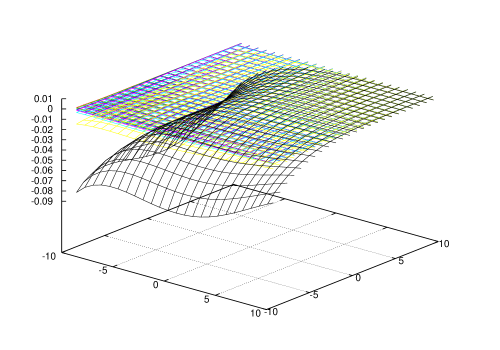
Figure 2: Evolution of dipole correlation defined by Balitsky-Kovchegov equation.
N 2 β ( k 1 , k 2 , Y ) subscript π 2 subscript π 1 subscript π 2 π N_{2}(k_{1},k_{2},Y) from l β o β g β ( k 1 2 ) , l β o β g β ( k 2 2 ) π π π superscript subscript π 1 2 π π π superscript subscript π 2 2
log(k_{1}^{2}),log(k_{2}^{2}) dependence for Y = 0 , 1 , 2 , 3 , 4 , 5 π 0 1 2 3 4 5
Y=0,1,2,3,4,5 from up to down
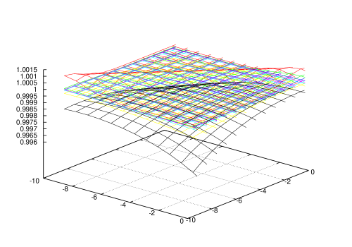
Figure 3: Evolution of dipole correlation defined by Balitsky-Kovchegov equation.
N 2 β ( k 1 , k 2 , Y ) / N 1 β ( k 1 , Y ) β N 1 β ( k 2 , Y ) + 1 subscript π 2 subscript π 1 subscript π 2 π subscript π 1 subscript π 1 π subscript π 1 subscript π 2 π 1 N_{2}(k_{1},k_{2},Y)/N_{1}(k_{1},Y)N_{1}(k_{2},Y)+1 from l β o β g β ( k 1 2 ) , l β o β g β ( k 2 2 ) π π π superscript subscript π 1 2 π π π superscript subscript π 2 2
log(k_{1}^{2}),log(k_{2}^{2}) dependence for Y = 0 , 1 , 2 , 3 , 4 , 5 π 0 1 2 3 4 5
Y=0,1,2,3,4,5 from up to down
It is clearly seen that β¨ T β ( k 1 , Y ) β T β ( k 2 , Y ) β© delimited-β¨β© π subscript π 1 π π subscript π 2 π \langle T(k_{1},Y)T(k_{2},Y)\rangle is smaller what value β¨ T β ( k 1 , Y ) β© β β¨ T β ( k 2 , Y ) β© delimited-β¨β© π subscript π 1 π delimited-β¨β© π subscript π 2 π \langle T(k_{1},Y)\rangle\langle T(k_{2},Y)\rangle supposed by mean field approximation. Moreover not only absolute difference between β¨ T β ( k 1 , Y ) β T β ( k 2 , Y ) β© delimited-β¨β© π subscript π 1 π π subscript π 2 π \langle T(k_{1},Y)T(k_{2},Y)\rangle and β¨ T β ( k 1 , Y ) β© β β¨ T β ( k 2 , Y ) β© delimited-β¨β© π subscript π 1 π delimited-β¨β© π subscript π 2 π \langle T(k_{1},Y)\rangle\langle T(k_{2},Y)\rangle does not vanish with Y π Y but so does relative difference.
This difference affect physical values related to dipole correlation such as elliptic flow v 2 subscript π£ 2 v_{2} and βback-forwardβ asymmetry in saturation model. Recently Balitsky-Kovchegov hierarchy was reformulated [5 ] using stochastic field theory. It was showed what (6 ) should contain additional βborderβ term which related to fluctuation. It therefore possible that N 2 β ( k 1 , k 2 , Y ) subscript π 2 subscript π 1 subscript π 2 π N_{2}(k_{1},k_{2},Y) behaviour will be changed drastically. This required further investigation.