DESY 05-260 Local Grand Unification

Abstract

In the standard model matter fields form complete representations of a grand unified group whereas Higgs fields belong to incomplete ‘split’ multiplets. This remarkable fact is naturally explained by ‘local grand unification’ in higher-dimensional extensions of the standard model. Here, the generations of matter fields are localized in regions of compact space which are endowed with a GUT gauge symmetry whereas the Higgs doublets are bulk fields. We realize local grand unification in the framework of orbifold compactifications of the heterotic string, and we present an example with $\mathrm{SO}(10)$ as a local GUT group, which leads to the supersymmetric standard model as an effective four-dimensional theory. We also discuss different orbifold GUT limits and the unification of gauge and Yukawa couplings.

11.25.Wx, 12.10.-g, 12.60.Jv, 11.25.Mj

1 Grand unification in $\boldsymbol{D>4}$ and doublet–triplet splitting

The standard model (SM) is a remarkably successful theory of the structure of matter. It is based on the gauge group $G_{\mathrm{SM}}=\mathrm{SU}(3)_{C}\times\mathrm{SU}(2)_{\mathrm{L}}\times\mathrm{U}(1)_{Y}$ and has three generations of matter transforming as

$$(\boldsymbol{3},\boldsymbol{2})_{1/6}+(\overline{\boldsymbol{3}},\boldsymbol{1})_{-2/3}+(\overline{\boldsymbol{3}},\boldsymbol{1})_{1/3}+(\boldsymbol{1},\boldsymbol{2})_{-1/2}+(\boldsymbol{1},\boldsymbol{1})_{1}\;.$$ (1)

The evidence for neutrino masses strongly supports the existence of right-handed neutrinos which are singlets under the SM gauge group. A crucial ingredient of the SM is further an $\mathrm{SU}(2)$ doublet of Higgs fields containing the Higgs boson which still remains to be discovered. From a theoretical perspective, one would like to amend the standard model by supersymmetry. Apart from stabilizing the hierarchy between the electroweak and Planck scales and providing a convincing explanation of the observed dark matter, the minimal supersymmetric extension of the standard model, the MSSM, predicts unification of the gauge couplings at the unification scale $M_{\mathrm{GUT}}\simeq 2\cdot 10^{16}\,\mathrm{GeV}$.

Even more than the unification of gauge couplings, the symmetries and the particle content of the standard model point towards grand unified theories (GUTs) [1]. Remarkably, one generation of matter, including the right-handed neutrino, forms a single spinor representation of $\mathrm{SO}(10)$ [3]. It therefore appears natural to assume an underlying $\mathrm{SO}(10)$ structure of the theory. The route of unification, continuing via exceptional groups, terminates at $\mathrm{E}_{8}$,

$$\mathrm{SO}(10)\subset\mathrm{E}_{6}\subset\mathrm{E}_{8}\;,$$ (2)

which is beautifully realized in the heterotic string [5].

An obstacle on the path towards unification are the Higgs fields, which are $\mathrm{SU}(2)$ doublets, while the smallest $\mathrm{SO}(10)$ representation containing Higgs doublets, the $\boldsymbol{10}$–plet, predicts additional $\mathrm{SU}(3)_{C}$ triplets. The fact that Higgs fields form incomplete ‘split’ GUT representations is particularly puzzling in supersymmetric theories where both matter and Higgs fields are chiral multiplets. The triplets cannot have masses below $M_{\mathrm{GUT}}$ since otherwise proton decay would be too rapid. This then raises the question why $\mathrm{SU}(2)$ doublets are so much lighter than $\mathrm{SU}(3)_{C}$ triplets. This is the notorious doublet-triplet splitting problem of ordinary 4D GUTs.

Higher-dimensional theories offer new possibilities for gauge symmetry breaking connected with the compactification to four dimensions. A simple and elegant scheme, leading to chiral fermions in four dimensions, is the compactification on orbifolds, first considered in string theories [7, 9], and more recently applied to GUT field theories [12]. In orbifold compactifications the gauge symmetry of the 4D effective theory is an intersection of larger symmetries at orbifold fixed points (cf. Fig. 1). Zero modes located at these fixed points all appear in the 4D theory and form therefore representations of the larger local symmetry groups. Zero modes of bulk fields, on the contrary, are only representations of the smaller 4D gauge symmetry and form in general ‘split multiplets’. Choosing now on some orbifold fixed points $\mathrm{SO}(10)$ as local symmetry, we obtain the picture of ‘local grand unification’ illustrated in Fig. 1. The SM gauge group is obtained as an intersection of different local GUT groups. Matter fields appear as $\boldsymbol{16}$–plets localized at the fixed points, whereas the Higgs doublets are associated with bulk fields, which provides a solution of the doublet-triplet splitting problem. In this way the structure of the standard model is naturally reproduced.

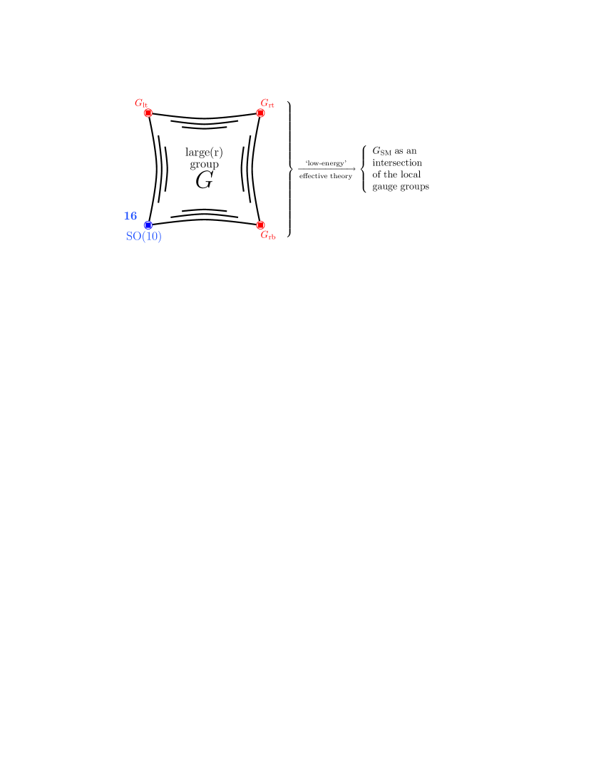
Figure 1: The picture of local grand unification. The gauge group $G$ is broken locally to different subgroups. Each of the local subgroups contains the standard model gauge group $G_{\mathrm{SM}}$ which emerges as an intersection of the local groups. ‘Brane’ fields which are confined to a region with certain symmetry have to come in complete matter multiplets of that symmetry. Hence, localized $\boldsymbol{16}$-plets of $\mathrm{SO}(10)$ are an attractive explanation of complete matter generations. Higgs doublets, on the other hand, are states which are not confined to an $\mathrm{SO}(10)$ region, and can therefore appear as ‘split multiplets’ in the low–energy spectrum.

2 Orbifold compactification of the heterotic string

‘Local grand unification’ naturally occurs in compactifications of the $\mathrm{E}_{8}\times\mathrm{E}_{8}$ heterotic string [5]. Six of the ten space-time dimensions are compactified on an orbifold [7, 9, 19]. Specifically, we consider $\mathbbm{Z}_{3}\times\mathbbm{Z}_{2}$ orbifold compactifications on the lattice $\Lambda_{\mathrm{G}_{2}\times\mathrm{SU}(3)\times\mathrm{SO}(4)}$, which is a product of three two-tori defined by the root vectors of $\mathrm{G}_{2}$, $\mathrm{SU}(3)$ and $\mathrm{SO}(4)$, respectively [20]. The $\mathbbm{Z}_{6}$ action is a rotation by $2\pi/6$ in the $\mathrm{G}_{2}$ plane, by $2\pi/3$ in the $\mathrm{SU}(3)$ plane and by $2\pi/2$ in the $\mathrm{SO}(4)$ plane. This $\mathbbm{Z}_{6}$ action has fixed points in the various planes as illustrated in Fig. 2.

The rotation in the compact dimensions is embedded into the gauge degrees of freedom. It acts as a shift, denoted by $V_{6}$, on the left-moving coordinates $X_{\mathrm{L}}^{I}$ ($1\leq I\leq 16$), i.e. upon a rotation in the internal space-time $X_{\mathrm{L}}^{I}$ transforms as $X_{\mathrm{L}}^{I}\to X_{\mathrm{L}}^{I}+V_{6}^{I}$. This shift satisfies $6V_{6}\in\Lambda_{\mathrm{E}_{8}\times\mathrm{E}_{8}}$, where $\Lambda_{\mathrm{E}_{8}\times\mathrm{E}_{8}}$ denotes the root lattice of $\mathrm{E}_{8}\times\mathrm{E}_{8}$, reflecting that the corresponding automorphism has order 6. In addition, some tori carry Wilson lines. For instance, a torus translation along one axis in the $\mathrm{SO}(4)$ torus is associated with a shift by $W_{2}$ which has degree two, i.e.  $2W_{2}\in\Lambda_{\mathrm{E}_{8}\times\mathrm{E}_{8}}$. A more detailed discussion can be found elsewhere [22, 20, 23, 24].

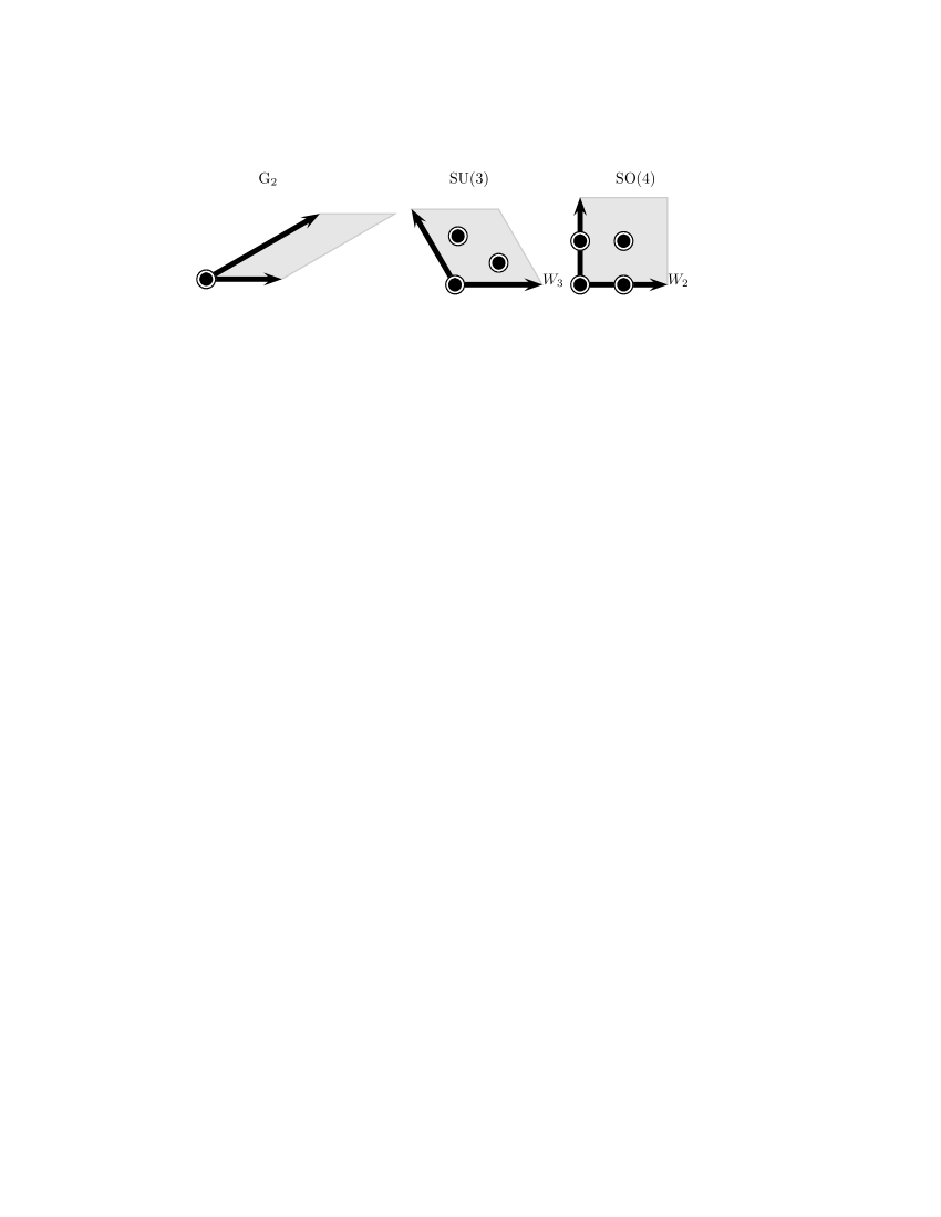
Figure 2: Root lattice $\Lambda_{G_{2}\times\mathrm{SU}(3)\times\mathrm{SO}(4)}$ and fixed points of the $\mathbbm{Z}_{6}$ action.

2.1 Orbifold construction kit

The orbifold action leads to local gauge symmetry breakdown at the fixed points. To see this, one analyzes locally the invariance conditions for the gauge fields $A_{\mu}^{p}$, corresponding to the generator $p\in\Lambda_{\mathrm{E}_{8}\times\mathrm{E}_{8}}$. For instance, at the origin in Fig. 2, the invariance condition requires that $A_{\mu}^{p}$ vanish unless the corresponding generator is ‘orthogonal’ to the local shift $V_{\mathrm{local}}=V_{6}$. This implies that any gauge boson not fulfilling $p\cdot V_{6}\equiv 0$ is projected out of the zero-mode spectrum. The remaining gauge bosons form a sub-algebra of the original $\mathrm{E}_{8}\times\mathrm{E}_{8}$. One can thus say that the origin carries a local gauge group.

Repeating the analysis at other fixed points leads in general to different local projection conditions. For instance, the local projection condition at the origin in the $\mathrm{G}_{2}$ and $\mathrm{SU}(3)$ tori and at the bottom right position in the $\mathrm{SO}(4)$ torus is the same as before except that the shift now gets amended by the Wilson line $W_{2}$, i.e. $V_{\mathrm{local}}=V_{6}+W_{2}$. This modified projection condition, $p\cdot V_{\mathrm{local}}\equiv 0$, implies a different local gauge group. An analogous analysis can be carried out for the remaining fixed points. The result is that each of the fixed points carries a local gauge group, and those local gauge groups are in general different. If two local shifts are equal, i.e. if the Wilson line corresponding to the translation connecting the two fixed points vanishes, the local gauge groups and their embedding into $\mathrm{E}_{8}\times\mathrm{E}_{8}$ coincide.

The gauge boson zero-modes consist of the gauge bosons surviving all local projection conditions simultaneously. In other words, the gauge group after compactification is an intersection of the local gauge groups. In the following, we shall focus on the possibility that this intersection is, up to $\mathrm{U}(1)$ factors and a ‘hidden sector gauge group’, the SM gauge group $G_{\mathrm{SM}}$ . It is crucial to note that each of the local gauge groups contains $G_{\mathrm{SM}}$ as a subgroup, i.e.

$$G_{\mathrm{SM}}\,\subsetneq\,G_{\mathrm{local}}\;.$$ (3)

This leads to the picture of ‘local grand unified theories’ where $G_{\mathrm{SM}}$ emerges as an intersection of different GUT groups residing at different fixed points.

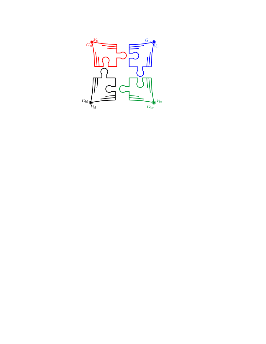
(a) Orbifold construction kit.

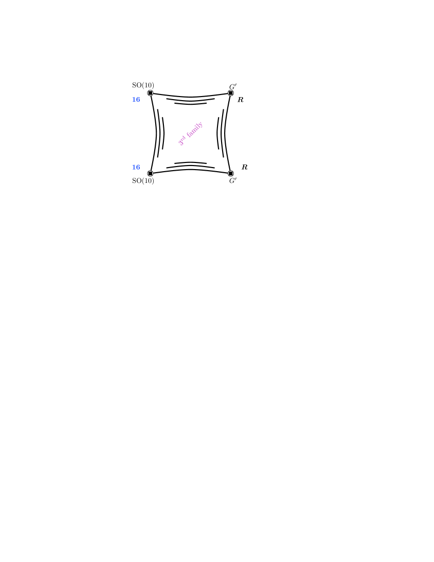
(b) $2+1$ family models.

Figure 3: (a) orbifolds can be constructed by combining ‘corners’ carrying a local gauge group emerging from the action of a local shift. (b) In $2+1$ family models, two families appear as $\boldsymbol{16}$–plets residing on fixed points with local $\mathrm{SO}(10)$ symmetry. The third family comes from elsewhere.

The geometry of a 2D orbifold can be visualized as follows (cf. [25]). The fundamental region of a $\mathbbm{Z}_{N}$ orbifold is one $N^{\mathrm{th}}$ of the fundamental region of the torus. One can fold it and identify the remaining edges. This yields a ‘pillow’ or ‘ravioli’ where the orbifold fixed points correspond to the corners (cf. Fig. 1).

The corners of the pillow serve as building blocks for the construction of an orbifold model. One starts at one corner with a local shift leading to a local gauge group. The simplest possibility is to combine identical corners which leads to an orbifold model without Wilson lines. In order to construct realistic orbifold models, one has to consider non-vanishing Wilson lines, i.e. combine corners with different gauge groups. Gluing these corners together leads to an orbifold model with Wilson lines (cf. Fig. 3(a)). Let us emphasize that one cannot combine these corners arbitrarily. Rather, there are severe constraints coming from modular invariance, which restrict the allowed Wilson lines (cf. [22]).

2.2 Localized $\boldsymbol{16}$–plets and 2+1 family models

The ‘orbifold construction kit’ described above is a helpful tool for model building. Note that each local GUT leads to local GUT representations. Among the zero modes, the representations of the first twisted sector $T_{1}$ play a special role. They correspond to ‘brane’ fields which are completely localized at the fixed points. In particular, they only feel the local gauge group and therefore are forced to furnish complete GUT representations.

An application of this observation to localized $\boldsymbol{16}$–plets of local $\mathrm{SO}(10)$ GUTs leads to a simple recipe for the construction of three generation models. One starts with a ‘corner’ which carries a local $\mathrm{SO}(10)$ and a $\boldsymbol{16}$–plet in the $T_{1}$ sector. This $\boldsymbol{16}$–plet will appear as a complete multiplet in the massless spectrum, even though the low-energy gauge group will be an intersection of $\mathrm{SO}(10)$ with other groups, and therefore only some subgroup of $\mathrm{SO}(10)$. As discussed above, this provides understanding of the fact that there are complete generations and split multiplets at the same time.

In the geometry introduced above there are only two shifts which produce a local $\mathrm{SO}(10)$ together with the $\boldsymbol{16}$–plets [27],

$$V_{6} = \left(\frac{1}{2},\frac{1}{2},\frac{1}{3},0,0,0,0,0\right)\left(\frac{1}{3},0,0,0,0,0,0,0\right)\;,$$

$$V_{6}^{\prime} = \left(\frac{1}{3},\frac{1}{3},\frac{1}{3},0,0,0,0,0\right)\left(\frac{1}{6},\frac{1}{6},0,0,0,0,0,0\right)\;.$$ (4)

In the following, we shall focus on $2+1$ family models, where two families come from two $\mathrm{SO}(10)$ corners while the third one comes from somewhere else (cf. Fig. 3(b)). This pattern has recently been explored in the context of Pati-Salam models [20]. In contrast to models with three families of localized $\boldsymbol{16}$–plets, in $2+1$ family models the third family and the Higgs originate partially from the untwisted sector. As we shall see, this leads naturally to a situation where the top Yukawa coupling is related to the gauge coupling. Note that an untwisted $\boldsymbol{16}$–plet, i.e. a bulk third family, occurs only in the $\mathrm{E}_{8}\times\mathrm{E}_{8}$ heterotic string and not in the $\mathrm{SO}(32)$ heterotic string.

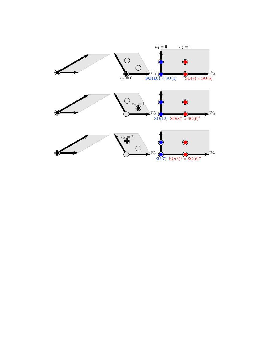
Figure 4: Local gauge groups up to $\mathrm{U}(1)$ factors and subgroups of the second $\mathrm{E}_{8}$. As indicated, the fixed point come in six pairs.

3 The MSSM from the heterotic string

3.1 Model definition and gauge groups

Let us now discuss a specific example [29]. We consider a compactification of the $\mathrm{E}_{8}\times\mathrm{E}_{8}$ heterotic string on the $\mathbbm{Z}_{3}\times\mathbbm{Z}_{2}$ orbifold described above. In order to obtain a $2+1$ family model, we require only two Wilson lines $W_{2}$ and $W_{3}$, while a possible third Wilson line associated with the ‘vertical’ translation in the $\mathrm{SO}(4)$ torus (cf. Fig. 2) is set to zero. In an orthonormal basis, the shift and the Wilson lines are given by

$$V_{6} = \left(\frac{1}{2},\frac{1}{2},\frac{1}{3},0,0,0,0,0\right)\,\left(\frac{1}{3},0,0,0,0,0,0,0\right)\;,$$

$$W_{2} = \left(\frac{1}{2},0,\frac{1}{2},\frac{1}{2},\frac{1}{2},0,0,0\right)\,\left(-\frac{3}{4},\frac{1}{4},\frac{1}{4},-\frac{1}{4},\frac{1}{4},\frac{1}{4},\frac{1}{4},-\frac{1}{4}\right)\;,$$

$$W_{3} = \left(\frac{1}{3},0,0,\frac{1}{3},\frac{1}{3},\frac{1}{3},\frac{1}{3},\frac{1}{3}\right)\,\left(1,\frac{1}{3},\frac{1}{3},\frac{1}{3},0,0,0,0\right)\;.$$ (5)

The twelve fixed points depicted in Fig. 4 come in six inequivalent pairs. They carry various local gauge groups whose intersection, which is the unbroken gauge group after compactification, is given by

$$G~{}=~{}G_{\mathrm{SM}}\times\left[\mathrm{SO}(6)\times\mathrm{SU}(2)\right]\times\mathrm{U}(1)^{8}\;.$$ (6)

Here, the brackets indicate a subgroup of the second $\mathrm{E}_{8}$. One of the $\mathrm{U}(1)$ factors is anomalous [30]. As a consequence, some fields charged under the anomalous $\mathrm{U}(1)$ attain vacuum expectation values (VEVs) which break this $\mathrm{U}(1)$ (cf. [31]). In our model there exist no fields which are charged only under the anomalous $\mathrm{U}(1)$. Hence, further $\mathrm{U}(1)$ factors are necessarily broken, which is phenomenologically attractive.

3.2 The massless spectrum

The zero modes of our model are given in Tab. 1, labeled by their quantum numbers w.r.t. the gauge group $G_{\mathrm{SM}}\times[\mathrm{SO}(6)\times\mathrm{SU}(2)]$. Further details such as the oscillator numbers will be presented elsewhere [24]. Here we only highlight some aspects of the spectrum.

name irrep count name irrep count $q_{i}$ $(\boldsymbol{3},\boldsymbol{2};\boldsymbol{1},\boldsymbol{1})_{1/6}$ 3 $\bar{u}_{i}$ $(\overline{\boldsymbol{3}},\boldsymbol{1};\boldsymbol{1},\boldsymbol{1})_{-2/3}$ 3 $\bar{d}_{i}$ $(\overline{\boldsymbol{3}},\boldsymbol{1};\boldsymbol{1},\boldsymbol{1})_{1/3}$ 7 $d_{i}$ $(\boldsymbol{3},\boldsymbol{1};\boldsymbol{1},\boldsymbol{1})_{-1/3}$ 4 $\bar{\ell}_{i}$ $(\boldsymbol{1},\boldsymbol{2};\boldsymbol{1},\boldsymbol{1})_{1/2}$ 5 $\ell_{i}$ $(\boldsymbol{1},\boldsymbol{2};\boldsymbol{1},\boldsymbol{1})_{-1/2}$ 8 $m_{i}$ $(\boldsymbol{1},\boldsymbol{2};\boldsymbol{1},\boldsymbol{1})_{0}$ 8 $\bar{e}_{i}$ $(\boldsymbol{1},\boldsymbol{1};\boldsymbol{1},\boldsymbol{1})_{1}$ 3 $s^{-}_{i}$ $(\boldsymbol{1},\boldsymbol{1};\boldsymbol{1},\boldsymbol{1})_{-1/2}$ 16 $s^{+}_{i}$ $(\boldsymbol{1},\boldsymbol{1};\boldsymbol{1},\boldsymbol{1})_{1/2}$ 16 $s^{0}_{i}$ $(\boldsymbol{1},\boldsymbol{1};\boldsymbol{1},\boldsymbol{1})_{0}$ 69 $h_{i}$ $(\boldsymbol{1},\boldsymbol{1};\boldsymbol{1},\boldsymbol{2})_{0}$ 14 $f_{i}$ $(\boldsymbol{1},\boldsymbol{1};\boldsymbol{4},\boldsymbol{1})_{0}$ 4 $\bar{f}_{i}$ $(\boldsymbol{1},\boldsymbol{1};\overline{\boldsymbol{4}},\boldsymbol{1})_{0}$ 4 $w_{i}$ $(\boldsymbol{1},\boldsymbol{1};\boldsymbol{6},\boldsymbol{1})_{0}$ 5

Table 1: The $G_{\mathrm{SM}}\times[\mathrm{SO}(6)\times\mathrm{SU}(2)]$ quantum numbers of the spectrum. The hypercharge is indicated by the subscript.

A key ingredient is the appearance of the ‘local GUTs’. In Tab. 2 we list the local gauge groups together with the local $T_{1}$ representations. As discussed in Section 2.2 our shift $V_{6}$ is chosen so as to produce two local $\boldsymbol{16}$–plets at $n_{2}=n_{3}=0,\ n_{2}^{\prime}=0,1$. Note that these are the only $T_{1}$ fields at $n_{2}=0$ which transform non-trivially under $G_{\mathrm{SM}}$. At $n_{2}=1$, there are $\boldsymbol{4}$–plets and $\overline{\boldsymbol{4}}$–plets w.r.t. $\mathrm{SO}(6)$ subgroups of the first $\mathrm{E}_{8}$. Although these $\mathrm{SO}(6)$ subgroups are embedded into $\mathrm{E}_{8}$ differently for different $n_{3}$, each $\boldsymbol{4}$–plet or $\overline{\boldsymbol{4}}$–plet gives rise to an $\mathrm{SU}(2)_{\mathrm{L}}$ doublet with zero hypercharge ($m_{i}$ of Tab. 1) and two non–Abelian singlets with opposite hypercharge ($s^{\pm}_{i}$ of Tab. 1). In particular, apart from the two $\boldsymbol{16}$–plets the $T_{1}$ states are vector–like w.r.t. $G_{\mathrm{SM}}$.

$n_{2}=0$ $n_{2}=1$ $n_{3}=0$ $\mathrm{SO}(10)\times\mathrm{SU}(2)^{2}\times\left[\mathrm{SO}(14)\right]$ $\mathrm{SO}(8)\times\mathrm{SO}(6)\times\left[\mathrm{SU}(7)\right]$ $\left(\boldsymbol{16},\boldsymbol{1},\boldsymbol{1};\boldsymbol{1}\right)$ $\left(\boldsymbol{1},\boldsymbol{4};\boldsymbol{1}\right)$ $\oplus\ 2\times\left(\boldsymbol{1},\boldsymbol{2},\boldsymbol{1};\boldsymbol{1}\right)\oplus\left(\boldsymbol{1},\boldsymbol{1},\boldsymbol{2};\boldsymbol{1}\right)$ $n_{3}=1$ $\mathrm{SO}(12)\times\left[\mathrm{SO}(8)\times\mathrm{SO}(6)\right]$ $\mathrm{SO}(8)^{\prime}\times\mathrm{SO}(6)^{\prime}\times\left[\mathrm{SU}(7)\right]$ $\left(\boldsymbol{1};\boldsymbol{8},\boldsymbol{1}\right)\oplus\left(\boldsymbol{1};\boldsymbol{1},\boldsymbol{4}\right)$ $\left(1,\boldsymbol{4};\boldsymbol{1}\right)$ $n_{3}=2$ $\mathrm{SU}(7)\times\left[\mathrm{SO}(8)\times\mathrm{SO}(6)\right]$ $\mathrm{SO}(8)^{\prime\prime}\times\mathrm{SO}(6)^{\prime\prime}\times\left[\mathrm{SO}(10)\times\mathrm{SU}(2)^{2}\right]$ $\left(\boldsymbol{1};\boldsymbol{1},\overline{\boldsymbol{4}}\right)$ $\left(\boldsymbol{1},\overline{\boldsymbol{4}};\boldsymbol{1},\boldsymbol{1},\boldsymbol{2}\right)$

Table 2: Local GUTs and local representations. The geometric interpretation of the ‘localization quantum numbers’ $n_{2}$ and $n_{3}$ is given in Fig. 4.

To understand the origin of the third generation, recall that the shift $V_{6}$ breaks the first $\mathrm{E}_{8}$ to $\mathrm{SO}(10)\times\mathrm{SU}(2)^{2}\times\mathrm{U}(1)$. Under this breaking, some internal components of the gauge bosons transforming in the coset $\mathrm{E}_{8}/[\mathrm{SO}(10)\times\mathrm{SU}(2)^{2}\times\mathrm{U}(1)]$ remain massless. An important property of this coset is that it contains $\boldsymbol{16}$–plets. In the $U_{1}$ and $U_{2}$ sectors we obtain $\mathrm{SO}(10)$ $\boldsymbol{16}$–plets, while in the $U_{3}$ sector we obtain $\mathrm{SO}(10)$ $\boldsymbol{10}$–plets. Here, the $U_{1}$, $U_{2}$ and $U_{3}$ sectors consist of the gauge bosons with spatial components in the direction of the $\mathrm{G}_{2}$, $\mathrm{SU}(3)$, and $\mathrm{SO}(4)$ torus, respectively. Due to the presence of Wilson lines, these $\mathrm{SO}(10)$ $\boldsymbol{16}$–plets and $\boldsymbol{10}$–plets are subject to further projections such that we finally obtain $(\overline{\boldsymbol{3}},\boldsymbol{1})_{-2/3}$ and $(\boldsymbol{1},\boldsymbol{1})_{1}$ w.r.t. $G_{\mathrm{SM}}$ from $U_{1}$, and $(\boldsymbol{3},\boldsymbol{2})_{1/6}$ from $U_{2}$. These states correspond to a $\boldsymbol{10}$–plet of $\mathrm{SU}(5)$. Together with localized states from higher twisted sectors, one obtains an additional complete generation. This seemingly miraculous completion of the third generation is related to the necessary SM anomaly cancellation.

In summary, the massless spectrum contains three generations, two of which originate from the $T_{1}$ sector and one being a mixture of states from $U$, $T_{2}$ and $T_{4}$. All other states are vector-like w.r.t. $G_{\mathrm{SM}}$. Thus we have

$$\text{matter:}~{}~{}~{}~{}3\times\boldsymbol{16}~{}~{}+~{}~{}\text{vector-like}\;.$$ (7)

One of the main problems of most known string models is the presence of exotic states at low energies. In our model the vector–like exotic states do not appear at low energies. Their mass terms are generated by the superpotential involving singlet fields and consistent with string selection rules [32, 34],

$$W~{}\supset~{}x_{i}\bar{x}_{j}\langle s_{a}^{0}s_{b}^{0}\dots\rangle\;.$$ (8)

The singlet fields acquire large VEVs yielding masses for all exotic states [29, 24]. Recently, an interesting class of heterotic string compactifications has been constructed where massless exotic states are absent from the beginning [36]. Their relation to the model described above remains to be clarified.

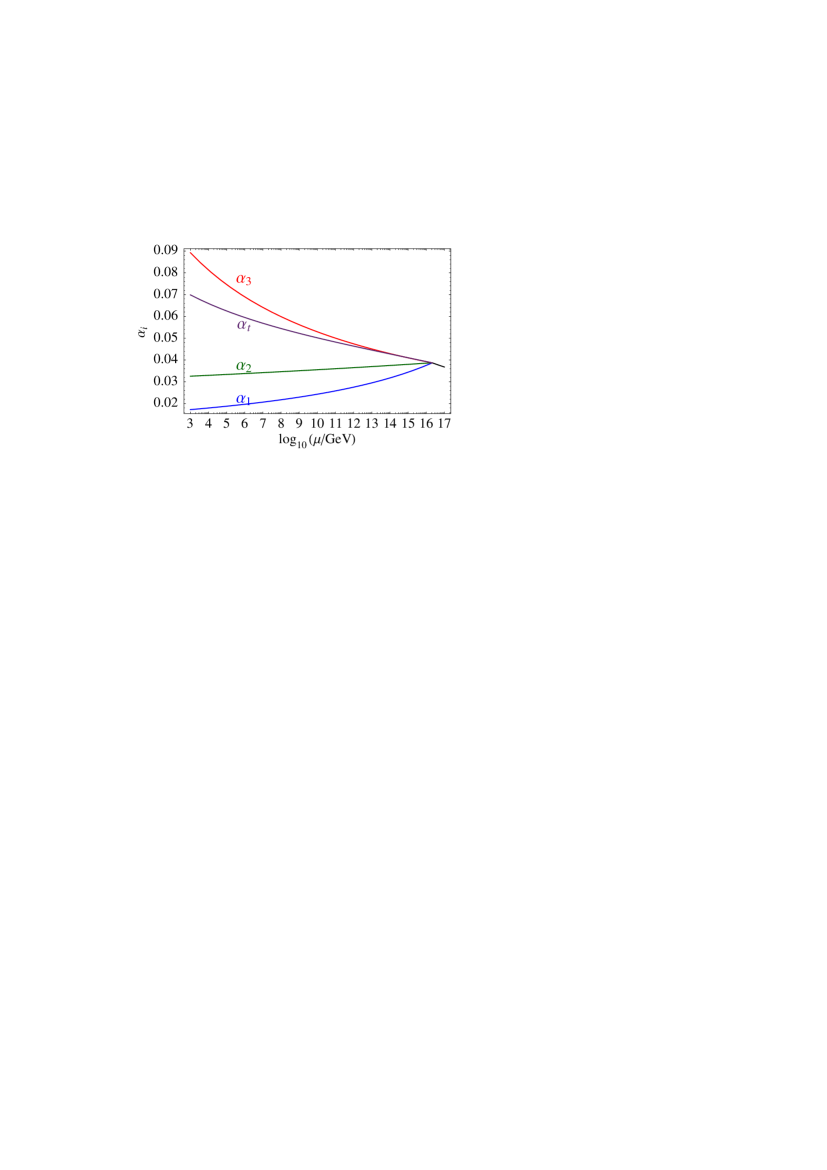
Figure 5: Illustration of gauge–Yukawa unification. The plot shows the MSSM evolution of $\alpha_{i}=g_{i}^{2}/(4\pi)$ and $\alpha_{t}=y_{t}^{2}/(4\pi)$ where $g_{i}$ denotes the gauge couplings and $y_{t}$ is the top Yukawa coupling.

3.3 Unification of couplings and flavour structure

Our model has no exotic states at low energies and admits TeV scale soft masses. Therefore, it is consistent with gauge coupling unification. Furthermore, the top–Yukawa coupling is related to the gauge coupling since the third generation originates partially from the untwisted sector. As described above, the $U_{3}$ zero modes descend from an $\mathrm{SO}(10)$ $\boldsymbol{10}$–plet, and give rise to two states $\ell_{1}$ and $\bar{\ell}_{1}$ with the quantum numbers of the MSSM Higgs doublets. The up–quark and the quark doublet of the third generation come from the untwisted sectors $U_{1}$ and $U_{2}$, respectively. The Yukawa coupling $U_{1}\,U_{2}\,U_{3}$ is a gauge interaction in 10D and its strength is given by the gauge coupling at the unification scale. One thus obtains the superpotential coupling

$$W~{}\supset~{}y_{t}\,q_{3}\,\bar{u}_{3}\,h_{u}\;,$$ (9)

with $y_{t}\simeq g$ at the GUT scale, as long as the MSSM ‘up–type’ Higgs is dominated by the $U_{3}$ state, $h_{u}\simeq\bar{\ell}_{1}$ (cf. Fig. 5). It is well known that this is consistent with the measured top mass. The Yukawa couplings involving the first two generation up–type quarks occur only through higher dimensional operators [29], which leads to the required suppression of these couplings.

The light down–type quarks $\bar{d}_{i}$ and lepton doublets $\ell_{i}$ are linear combinations of states from various twisted and untwisted sectors. A similar setup has recently been proposed in the context of orbifold GUTs [39]. There, it has been shown that a mixing of the light leptons (down–type quarks) with additional heavy leptons (down–type quarks) can lead to the observed large neutrino mixings together with small CKM mixings in the quark sector. In our heterotic string model an analogous mixing occurs. A more detailed analysis of phenomenological aspects of the model will be presented elsewhere.

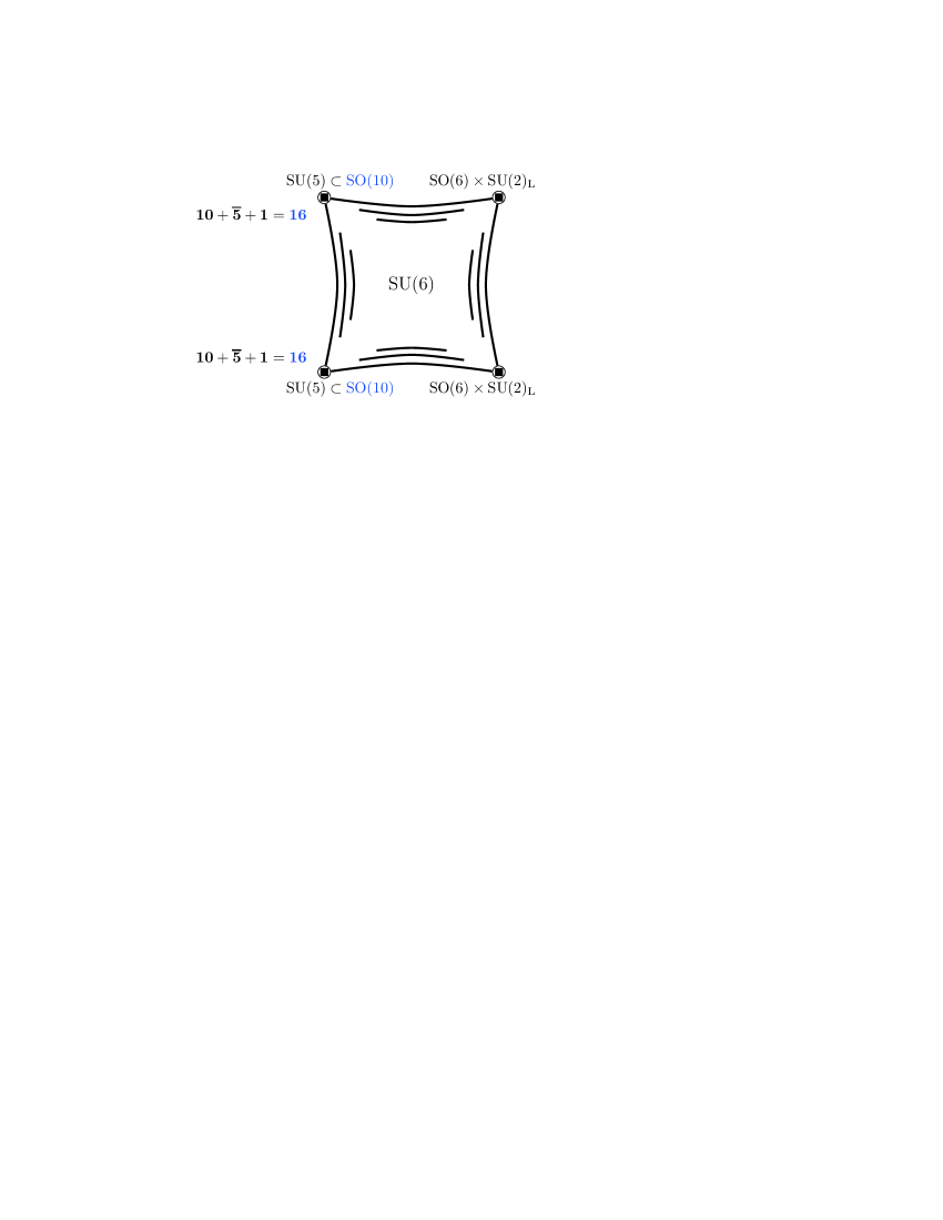
(a) $\mathrm{SO}(4)$ plane large.

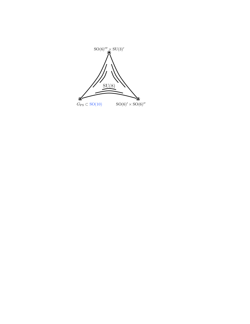
(b) $\mathrm{SU}(3)$ plane large.

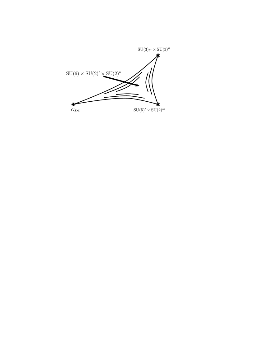
(c) $\mathrm{G}_{2}$ plane large.

Figure 6: Orbifold GUT limits. Only subgroups of the first $\mathrm{E}_{8}$ are shown, and $\mathrm{U}(1)$ factors are omitted.

3.4 Orbifold GUT limits

One of the main motivations for revisiting orbifold compactifications of the heterotic string is the phenomenological success of orbifold GUTs. It is therefore interesting to study orbifold GUT limits of the model, which correspond to anisotropic compactifications where some radii are significantly larger than the others. Such anisotropy may mitigate the discrepancy between the GUT and the string scales [40]. In the energy range between the compactification scale and the string scale one obtains an effective higher-dimensional field theory.

We focus on $4+2$–dimensional orbifold GUT limits, and keep only subgroups of the first $\mathrm{E}_{8}$ factor in the subsequent analysis. As an example, consider the case that the compactification radii of the $\mathrm{SO}(4)$ plane are larger than the others. For energies in the range $R_{\mathrm{SO}(4)}^{-1}<E<R_{\mathrm{G}_{2},\mathrm{SU}(3)}^{-1}$ the model is described by an effective six–dimensional theory. The local gauge groups at the fixed points and the gauge group in the bulk are obtained by imposing the following projection conditions on the gauge bosons labeled by $p$:

bulk $$: 2V_{6}\cdot p~{}\equiv~{}0\;, W_{3}\cdot p~{}\equiv~{}0\;,$$

$$n_{2}=0 : V\cdot p~{}\equiv~{}0\;, W_{3}\cdot p~{}\equiv~{}0\;,$$

$$n_{2}=1 : (V+W_{2})\cdot p~{}\equiv~{}0\;, W_{3}\cdot p~{}\equiv~{}0\;.$$ (10)

This leads to the bulk group $\mathrm{SU}(6)$ and to the ‘local GUTs’ $\mathrm{SU}(5)$ at $n_{2}=0$ and $\mathrm{SO}(6)\times\mathrm{SU}(2)_{\mathrm{L}}$ at $n_{2}=1$, respectively (cf. Fig. 6 (a)). The two fixed points with $n_{2}=0$ carry one generation each. The appearance of these complete generations cannot be fully understood in the 6D orbifold GUT limit. To have deeper understanding one has to zoom into the smaller dimensions and unravel the underlying $\mathrm{SO}(10)$ gauge symmetry. An important property of this limit is that the bulk $\mathrm{SU}(6)$ is a simple group containing $G_{\mathrm{SM}}$. Hence the running of the gauge couplings in six dimensions does not discriminate between the subgroups of $G_{\mathrm{SM}}$. This supports the picture of gauge coupling unification at the compactification scale.

An analogous analysis can be carried out when the $\mathrm{SU}(3)$ torus is larger than the other tori. In this case, one obtains the orbifold GUT shown in Fig. 6 (b) as an effective theory. The first two generations are localized at the fixed point with the Pati–Salam group $G_{\mathrm{PS}}=\mathrm{SO}(6)\times\mathrm{SU}(2)_{\mathrm{L}}\times\mathrm{SU}(2)_{\mathrm{R}}$ as an unbroken local GUT. Again, the bulk group is simple and contains all SM group factors.

In the limit where the $\mathrm{G}_{2}$ torus is large, the first two generations reside at the fixed point with unbroken gauge symmetry $G_{\mathrm{SM}}$ (cf. Fig. 6 (c)). In this case, $\mathrm{SU}(3)_{C}\times\mathrm{SU}(2)_{\mathrm{L}}$ is a subgroup of the bulk group $\mathrm{SU}(6)$, but hypercharge is not fully contained in this $\mathrm{SU}(6)$. However, this does not lead to the running or threshold corrections which discriminate between the hypercharge and the simple SM subgroups because of $N=4$ supersymmetry in the bulk, implying vanishing $\beta$–functions.

In summary, we find that all orbifold limits are consistent with gauge coupling unification up to possible logarithmic corrections coming from states localized at the fixed points. The different geometries have, however, important consequences for the values of the gauge couplings at the compactification scale and also for the pattern of the Yukawa couplings. These issues will be analyzed in more detail elsewhere.

4 Summary

The quest for unification is a central theme of particle physics. In a bottom–up approach, starting from the standard model, one is first led to conventional 4D GUTs. Among the GUT groups, $\mathrm{SO}(10)$ is singled out since one matter generation, including the right–handed neutrino, forms an irreducible representation of $\mathrm{SO}(10)$, the $\boldsymbol{16}$–plet. The route of unification, continuing via exceptional groups, terminates at $\mathrm{E}_{8}$.

An attractive starting point for a unified theory including gravity is, in a top–down approach, the heterotic string with the gauge group $\mathrm{E}_{8}\times\mathrm{E}_{8}$. In its orbifold compactifications, GUT groups appear locally at orbifold fixed points. We have presented an example with local $\mathrm{SO}(10)$ symmetry and localized $\boldsymbol{16}$–plets from the twisted sectors. The standard model gauge group is obtained as an intersection of different local $\mathrm{E}_{8}$ subgroups. The model has three quark–lepton generations, one pair of Higgs doublets and no exotic matter.

Acknowledgements. It is a pleasure to thank T. Kobayashi, M. Lindner, J. Louis, H. P. Nilles and S. Stieberger for valuable discussions. W. B. thanks the organizers of the GUSTAVOFEST for arranging an enjoyable and stimulating Symposium in Honor of Gustavo C. Branco. M. R. is deeply indebted to A. Wisskirchen for technical support. This work was partially supported by the European Union 6th Framework Program MRTN-CT-2004-503369 “Quest for Unification” and MRTN-CT-2004-005104 “ForcesUniverse”.

References

- [1] H. Georgi, S. L. Glashow, Phys. Rev. Lett. 32 (1974), 438
- [2] J. C. Pati, A. Salam, Phys. Rev. D10 (1974), 275
- [3] H. Georgi, in: Particles and Fields 1974, ed. C. E. Carlson (AIP, NY, 1975) p. 575
- [4] H. Fritzsch, P. Minkowski, Ann. Phys. 93 (1975), 193
- [5] D. J. Gross, J. A. Harvey, E. J. Martinec, R. Rohm, Phys. Rev. Lett. 54 (1985), 502
- [6] D. J. Gross, J. A. Harvey, E. J. Martinec, R. Rohm, Nucl. Phys. B256 (1985), 253
- [7] L. J. Dixon, J. A. Harvey, C. Vafa, E. Witten, Nucl. Phys. B261 (1985), 678
- [8] L. J. Dixon, J. A. Harvey, C. Vafa, E. Witten, Nucl. Phys. B274 (1986), 285
- [9] L. E. Ibáñez, H. P. Nilles, F. Quevedo, Phys. Lett. B187 (1987), 25
- [10] L. E. Ibáñez, H. P. Nilles, F. Quevedo, Phys. Lett. B192 (1987), 332
- [11] L. E. Ibáñez, J. E. Kim, H. P. Nilles, F. Quevedo, Phys. Lett. B191 (1987), 282
- [12] Y. Kawamura, Prog. Theor. Phys. 103 (2000), 613
- [13] Y. Kawamura, Prog. Theor. Phys. 105 (2001), 999
- [14] G. Altarelli, F. Feruglio, Phys. Lett. B511 (2001), 257
- [15] L. J. Hall, Y. Nomura, Phys. Rev. D64 (2001), 055003
- [16] A. Hebecker, J. March-Russell, Nucl. Phys. B613 (2001), 3
- [17] T. Asaka, W. Buchmüller, L. Covi, Phys. Lett. B523 (2001), 199
- [18] L. J. Hall, Y. Nomura, T. Okui, D. R. Smith, Phys. Rev. D65 (2002), 035008
- [19] Y. Katsuki, Y. Kawamura, T. Kobayashi, N. Ohtsubo, Y. Ono, K. Tanioka, Nucl. Phys. B341 (1990), 611
- [20] T. Kobayashi, S. Raby, R.-J. Zhang, Phys. Lett. B593 (2004), 262
- [21] T. Kobayashi, S. Raby, R.-J. Zhang, Nucl. Phys. B704 (2005), 3
- [22] S. Förste, H. P. Nilles, P. K. S. Vaudrevange, A. Wingerter, Phys. Rev. D70 (2004), 106008
- [23] W. Buchmüller, K. Hamaguchi, O. Lebedev, M. Ratz, Nucl. Phys. B712 (2005), 139
- [24] W. Buchmüller, K. Hamaguchi, O. Lebedev, M. Ratz, in preparation
- [25] F. Quevedo, hep-th/9603074
- [26] A. Hebecker, M. Ratz, Nucl. Phys. B670 (2003), 3
- [27] Y. Katsuki, et al., DPKU-8810-REV
- [28] Y. Katsuki, et al., DPKU-8904
- [29] W. Buchmüller, K. Hamaguchi, O. Lebedev, M. Ratz, hep-ph/0511035
- [30] M. Dine, N. Seiberg, E. Witten, Nucl. Phys. B289 (1987), 589
- [31] G. Cleaver, M. Cvetic̆, J. R. Espinosa, L. L. Everett, P. Langacker, Nucl. Phys. B525 (1998), 3
- [32] S. Hamidi, C. Vafa, Nucl. Phys. B279 (1987), 465
- [33] L. J. Dixon, D. Friedan, E. J. Martinec, S. H. Shenker, Nucl. Phys. B282 (1987), 13
- [34] A. Font, L. E. Ibáñez, H. P. Nilles, F. Quevedo, Nucl. Phys. B307 (1988), 109
- [35] A. Font, L. E. Ibáñez, H. P. Nilles, F. Quevedo, Phys. Lett. B210 (1988), 101
- [36] V. Braun, Y.-H. He, B. A. Ovrut, T. Pantev, Phys. Lett. B618 (2005), 252
- [37] V. Bouchard, R. Donagi, hep-th/0512149
- [38] V. Braun, Y.-H. He, B. A. Ovrut, T. Pantev, hep-th/0512177
- [39] T. Asaka, W. Buchmüller, L. Covi, Phys. Lett. B563 (2003), 209
- [40] E. Witten, Nucl. Phys. B471 (1996), 135
- [41] A. Hebecker, M. Trapletti, Nucl. Phys. B713 (2005), 173.