Recoil corrections in the hydrogen isoelectronic sequence

Abstract

A version of the Bethe-Salpeter equation appropriate for calculating recoil corrections in highly charged hydrogenlike ions is presented. The nucleus is treated as a scalar particle of charge $Z$, and the electron treated relativistically. The known recoil corrections of order ${m^{2}\over M}(Z\alpha)^{4}$ are derived in both this formalism and in NRQED.

I introduction

Precision tests of QED in atoms were first carried out for hydrogen, and have been extended to other one-electron systems such as positronium and muonium, as well as helium Drakebook , lithium lithium , and even beryllium beryllium . In all these cases the nuclear charge $Z$ is low, so the basic expansion parameter of bound state QED, $Z\alpha$, is a small quantity. For this reason techniques in which the smallness of this parameter is exploited have been refined in sophistication over the years, culminating in the present widespread use of effective field theories such as NRQED NRQED and the effective Hamiltonian method Pach1 . However, at the same time experiments of increasing precision have been carried out on both highly charged hydrogenlike ions and also ions with more electrons, where as an example of the accuracy achieved at the highest $Z$ we note the recent determination Beiersdorfer of the $2p_{1/2}-2s_{1/2}$ transition energy in lithiumlike uranium,

$$E_{2p_{1/2}}-E_{2s_{1/2}}=280.645(15)~{}{\rm eV}.$$ (1)

As the expansion parameter $Z\alpha$ is no longer small in this case, techniques in which an expansion in it is avoided are necessary. In the non-recoil limit, in which the nuclear mass is taken to infinity, Furry representation QED Furry allows a systematic Feynman diagram based treatment of highly charged ions. A central structure in this approach is the electron propagator in a Coulomb field, the Dirac-Coulomb propagator, which satisfies the equation

$$\left[\left(E+{Z\alpha\over{\left|\vec{x}\right|}}\right)\gamma_{0}+i\vec{\gamma}\cdot\vec{\nabla}-m\right]S_{F}(\vec{x},\vec{y};E)=\delta^{3}\left(\vec{x}-\vec{y}\right).$$ (2)

As first pointed out by Wichmann and Kroll W-K for the vacuum polarization, and by Brown, Langer and Schaefer BLS for the self energy, treating this propagator exactly using numerical methods allows a determination of the Lamb shift that automatically accounts for all orders of an expansion in $Z\alpha$.

When applied to lithiumlike uranium, use of this propagator gives a one-loop Lamb shift contribution (including screening corrections) to the $2p_{1/2}-2s_{1/2}$ splitting of -41.793 eV, which when combined with the nonradiative energy shift of 322.231 eV leaves a 0.207 eV discrepancy with experiment. This can be used to infer the two-loop Lamb shift, which has recently been calculated for the ground state of hydrogenic ions 2loop , but before this can be done recoil terms, the subject we wish to address in this paper, must be reliably calculated.

Recoil effects have of course been treated for low $Z$ atoms, but again the techniques cannot be directly extended to high $Z$ ions. The general level of treatment of these small corrections in this latter case is to scale the overall energies by a factor of $\mu/m$, where the reduced mass $\mu$ is defined in the usual way in terms of the electron mass $m$ and the nuclear mass $M$,

$$\mu={mM\over m+M}.$$ (3)

This has a relatively small effect for the transition we are discussing, amounting to only -0.006 eV, below the experimental error. A larger effect comes from the mass-polarization operator,

$$H_{MP}=\sum_{i<j}{\vec{p}_{i}\cdot\vec{p}_{j}\over M}.$$ (4)

When this term is evaluated in a realistic potential it contributes -0.081 eV, for a total lowest order effect of -0.087 eV, 42 percent of the discrepancy. To accurately infer the two-loop Lamb shift, a more sophisticated treatment of recoil effects is clearly needed. The only such treatment we are aware of is that given by Shabaev Victor and collaborators Victors , who in fact find significant corrections to the above result. The present paper is intended to lay the groundwork for an alternative approach. We will restrict our attention to the hydrogen isoelectronic sequence, and in addition restrict our attention to diagrams that contribute in the low $Z$ case to order $m^{2}(Z\alpha)^{4}/M$, leaving the treatment of a more complete set of diagrams, along with the treatment of the many-electron problem, for a later paper.

While considerable progress has been made in QED in recent years with the use of effective field theories, these rely on expanding around the nonrelativistic Schrödinger equation, which, as just discussed, is not appropriate for highly charged ions. However, the Bethe-Salpeter formalism B-S , introduced first to treat the binding of the deuteron and shortly afterwards applied to the atomic problem by Salpeter Salpeter , allows the problem to be treated in a systematic manner. However, this equation is famously difficult to apply, and most applications rely on expanding around the nonrelativistic limit, which we wish to avoid.

The treatment given by Shabaev is fairly complicated, and we wish to provide a cross check by introducing as simple a formalism as possible. This can be done by slightly modifying a formalism introduced by Lepage Lepage , and it is this approach we will now describe.

The plan of the paper is to set up in the following section a three-dimensional formalism equivalent in rigor to the Bethe-Salpeter equation. In the next section the one and two photon exchange diagrams that contribute to order $m^{2}(Z\alpha)^{4}/M$ will be evaluated in Coulomb gauge, and their nonrelativistic limit will be taken. This will be followed by a NRQED treatment, and in the conclusion we will describe how a calculation relevant to highly charged ions can be carried out.

II Formalism

It has been known for quite some time Fronsdal that there is an arbitrary number of bound state equations equivalent in rigor to the original form of the Bethe-Salpeter equation, but that are effectively three-dimensional. Many practical calculations have used formulations that also incorporate the Schrödinger equation Caswell-Lepage , Adkins-Fell . However, for the problem we are considering a relativistic approach is demanded. We note that a fairly detailed discussion of a number of notational and formal issues involved with the use of three-dimensional forms of the Bethe-Salpeter equation is given in Ref. Adkins-Fell , to which we refer the reader interested in more detail.

The spectrum of many high-$Z$ ions has been studied, and it would be impractical to consider the differing spins of each nucleus. For this reason we simply treat the nucleus as a spinless particle of charge $Z|e|$. The Feynman rules for the electrodynamics of a spin-0 particle involve the coupling $iZ|e|(p+p^{\prime})_{\mu}$ for the one-photon vertex, and $2i(Ze)^{2}g_{\mu\nu}$ for the seagull vertex. The $\mu=0$ component of the one-photon vertex for a nucleus close to mass shell will then be dominated by the factor $2M$, where $M$ is the mass of the nucleus. Hyperfine effects associated with nuclear spin can be treated separately. We can also model the finite size of the nucleus by replacing the nuclear charge $Z$ with a form factor $Z({\vec{q}\,}^{2})$ if desired, but this will not be done in this paper.

We now consider the truncated two-particle Green’s function for the scattering of an electron and nucleus. We define the initial and final electron three-momenta as $\vec{k}$ and $\vec{l}$ respectively, and work in the center of mass so that the corresponding nuclear momenta are $-\vec{k}$ and $-\vec{l}$. For the fourth component of momentum we choose $E_{1}+k_{0}$ and $E_{1}+l_{0}$ for the electron line and $E_{2}-k_{0}$ and $E_{2}-l_{0}$ for the nuclear line, where $E_{1}$ and $E_{2}$ will be chosen close to the electron and nuclear masses, and when the total center of mass energy $E=E_{1}+E_{2}$ is a bound state energy a pole will be present. The formalism to be described below in its simplest form leads to a perturbation expansion about $E_{1}=\epsilon$ and $E_{2}=M$, with $\epsilon$ equal to the Dirac bound state energy,

$${\epsilon} = m\Biggl{[}1+\Biggl{(}\frac{Z\alpha}{n-(j+1/2)+\sqrt{(j+1/2)^{2}-(Z\alpha)^{2}}}\Biggr{)}^{2}\Biggr{]}^{-1/2}$$ (5)

$$= m\Biggl{\{}1-\frac{(Z\alpha)^{2}}{2n^{2}}-\frac{(Z\alpha)^{4}}{2n^{3}}\Bigl{(}\frac{1}{j+1/2}-\frac{3}{4n}\Bigr{)}+O((Z\alpha)^{6})\Biggr{\}}\,,$$ (6)

giving a total bound state energy $E=M+\epsilon=M+m-m\frac{(Z\alpha)^{2}}{2n^{2}}+...$ However, since this does not incorporate the known reduced mass dependence of the nonrelativistic binding energy, we will instead arrange the formalism so that $E_{1}={\cal E}={\mu\over m}\epsilon$ and $E_{2}=M+m-\mu\equiv\tilde{M}$. We incorporate these energies into the four-vectors $P_{1}=({\cal E},\vec{0}\,)$ and $P_{2}=(\tilde{M},\vec{0}\,)$. If we also define four vectors $k=(k_{0},\vec{k}\,)$ and $l=(l_{0},\vec{l}\,)$, the initial electron and nuclear momenta are $P_{1}+k$, $P_{2}-k$, and the final momenta $P_{1}+l$, $P_{2}-l$. The truncated two particle Green’s function obeys the equation

$$G_{T}(P_{1}+k,P_{2}-k;P_{1}+l,P_{2}-l)=iK(P_{1}+k,P_{2}-k;P_{1}+l,P_{2}-l)+$$

$$\int{d^{4}q\over(2\pi)^{4}}K(P_{1}+k,P_{2}-k;P_{1}+q,P_{2}-q)S(q)G_{T}(P_{1}+q,P_{2}-q;P_{1}+l,P_{2}-l),$$ (7)

where $K$ represents all two-particle irreducible kernels and the spin-1/2–spin-0 two-particle propagator has the form

$$S(q)=\frac{i}{\gamma(P_{1}+q)-m+i\epsilon}\times\frac{i}{(P_{2}-q)^{2}-M^{2}+i\epsilon}\,.$$ (8)

For brevity in the following we will write the above as

$$G_{T}(k,l;E)=iK(k,l;E)+\int{d^{4}q\over(2\pi)^{4}}K(k,q;E)S(q)G_{T}(q,l;E).$$ (9)

The main point of all simplifications of the Bethe-Salpeter formalism is that we can replace the relatively complicated two-particle propagator $S$ with a simplified form $S_{0}$ and write

$$G_{T}(k,l;E)=i\bar{K}(k,l;E)+\int{d^{4}q\over(2\pi)^{4}}\bar{K}(k,q;E)S_{0}(q)G_{T}(q,l;E),$$ (10)

which serves to define $\bar{K}$ through

$$\bar{K}(k,l;E)=K(k,l;E)+\int{d^{4}q\over(2\pi)^{4}}K(k,q;E)(S(q)-S_{0}(q))K(q,l;E)+$$

$$\int{d^{4}q\over(2\pi)^{4}}\int{d^{4}p\over(2\pi)^{4}}K(k,q;E)(S(q)-S_{0}(q))K(q,p;E)(S(p)-S_{0}(p))K(p,l;E)+...$$ (11)

Our choice for $S_{0}(q)$ is

$$S_{0}(q) = {\pi\delta(q_{0})\over\tilde{M}}\frac{i}{{\cal E}\gamma_{0}-\vec{\gamma}\cdot\vec{q}-\mu+i\epsilon}$$ (12)

$$\equiv {i\pi\delta(q_{0})\over\tilde{M}}S_{0}(\vec{q}).$$

As mentioned above, we could have chosen another form with ${\cal E}$ and $\mu$ replaced with $\epsilon$ and $m$, which would lead to the Dirac equation with mass $m$ in the $M\rightarrow\infty$ limit. Our method will lead to a Dirac equation with reduced mass $\mu$ in that limit. We note that this method of building in the reduced mass is relatively simple, in particular requiring no rescaling of coupling constants. The delta function we have chosen differs from that of Ref. Lepage , in which a delta function that puts the nucleus on mass shell is chosen. While the latter choice has a number of advantages when Feynman gauge is used, we use Coulomb gauge in this calculation, and putting the nucleus on-shell is not needed. At this point we can go to a completely three-dimensional formalism by choosing $k_{0}=l_{0}=0$, a choice that has no effect on the location of the bound state poles, and which allows us to replace the four vectors $k$ and $l$ with $\vec{k}$ and $\vec{l}$. In this case Eq. (10) takes the three-dimensional form

$$G_{T}(\vec{k},\vec{l};E)=i\bar{K}(\vec{k},\vec{l};E)+{1\over 2\tilde{M}}\int{d^{3}q\over(2\pi)^{3}}i\bar{K}(\vec{k},\vec{q};E)S_{0}(\vec{q}\,)G_{T}(\vec{q},\vec{l};E).$$ (13)

One gets to a bound state equation by creating an untruncated Green’s function $\bar{G}(\vec{k},\vec{l};E)$ defined through

$$\bar{G}(\vec{k},\vec{l};E)={1\over 2\tilde{M}}S_{0}(\vec{k}\,)(2\pi)^{3}{\delta}^{3}(\vec{k}-\vec{l}\,)+{1\over 4\tilde{M}^{2}}S_{0}(\vec{k}\,)G_{T}(\vec{k},\vec{l};E)S_{0}(\vec{l}\,)$$ (14)

that satisfies

$$\bar{G}(\vec{k},\vec{l};E)={1\over 2\tilde{M}}S_{0}(\vec{k}\,)(2\pi)^{3}{\delta}^{3}(\vec{k}-\vec{l}\,)+S_{0}(\vec{k}\,){1\over 2\tilde{M}}\int{d^{3}q\over(2\pi)^{3}}i\bar{K}(\vec{k},\vec{q};E)\bar{G}(\vec{q},\vec{l};E).$$ (15)

While this function differs from the Bethe-Salpeter untruncated Green’s function, it has poles at exactly the same total energy comment1 . In order to obtain a solvable problem, we now introduce the simpler equation

$$G_{0}(\vec{k},\vec{l};E)={1\over 2\tilde{M}}S_{0}(\vec{k}\,)(2\pi)^{3}{\delta}^{3}(\vec{k}-\vec{l}\,)+S_{0}(\vec{k}\,){1\over 2\tilde{M}}\int{d^{3}q\over(2\pi)^{3}}iK_{1C}(\vec{k},\vec{q};E)G_{0}(\vec{q},\vec{l};E),$$ (16)

which can be written, because the kernel $K_{1C}$ for one Coulomb photon exchange is

$$K_{1C}={4\pi iZ\alpha\over{|\vec{k}-\vec{q}\,|^{2}}}2\tilde{M}\gamma_{0},$$ (17)

as

$$({\cal E}\gamma_{0}-\vec{\gamma}\cdot\vec{k}-\mu)G_{0}(\vec{k},\vec{l};E)={1\over 2\tilde{M}}(2\pi)^{3}{\delta}^{3}(\vec{k}-\vec{l}\,)-4\pi Z\alpha\int\frac{d^{3}q}{(2\pi)^{3}}{1\over|\vec{k}-\vec{q}\,|^{2}}\gamma^{0}G_{0}(\vec{q},\vec{l};E),$$ (18)

where we have multiplied by $S^{-1}_{0}(\vec{k}\,)$.

In the following section we will discuss the effect of expanding $\bar{G}$ about $G_{0}$, but here restrict our attention to the latter function, which, except for the factor of ${1\over 2\tilde{M}}$ multiplying the delta function, is precisely the momentum space form of Eq. (2) with the electron mass replaced with the reduced mass. It has the spectral representation

$$G_{0}(\vec{k},\vec{l};E)=\sum_{n}{\psi_{n}(\vec{k}\,)\bar{\psi}_{n}(\vec{l}\,)\over{{\cal E}-{\cal E}_{n}}},$$ (19)

where $\psi_{n}(\vec{l})$ is the solution to the Dirac equation with the usual normalization factor multiplied by $\sqrt{1\over 2\tilde{M}}$, and has poles when $E=\tilde{M}+{\cal E}_{n}\equiv E_{0}$. To illustrate, the ground state (g) wave function has energy

$${E_{0}}^{g}=\tilde{M}+\mu\gamma$$ (20)

where $\gamma=\sqrt{1-(Z\alpha)^{2}}$, and the form

$${\psi_{0}}^{g}(\vec{p}\,)=\sqrt{1\over 2\tilde{M}}(\mu Z\alpha)^{-{3\over 2}}\left(\begin{array}[]{c}g(p)\chi_{-1\mu}(\hat{p})\\ {\vec{\sigma}\cdot\vec{p}\over 2\mu}f(p)\chi_{-1\mu}(\hat{p})\end{array}\right),$$ (21)

where $g(p)$ and $f(p)$ can be expressed in terms of the dimensionless variable $q=p/(\mu Z\alpha)$,

$$g(p) = {N\over 2q}{\rm sin}(\theta(1+\gamma))[1+q^{2}]^{-(1+\gamma)/2}$$

$$f(p) = {N\over q^{3}(1+\gamma)}\left[{{\rm sin}(\gamma\theta)\over\gamma}\sqrt{1+q^{2}}-q{\rm cos}(\theta(1+\gamma))\right][1+q^{2}]^{-(1+\gamma)/2}.$$ (22)

Here $\theta\equiv{\rm tan}^{-1}q$ and the normalization factor $N$ is

$$N=2^{\gamma+3}\pi\Gamma(1+\gamma)\sqrt{(1+\gamma)\over\Gamma(1+2\gamma)}.$$ (23)

The $\chi_{\kappa}$’s are two-component eigenfunctions of $J^{2}$, $J_{z}$, $L^{2}$, and $S^{2}$ and are labeled by $\kappa=\mp(j+1/2)$ for $j=\ell\pm 1/2$ and $\mu$, the quantum number corresponding to $J_{z}$. The spherical spinors are normalized so that $\chi^{\dagger}\chi$, when integrated over solid angle, gives one. In the following we adopt the convention of working with Dirac wave functions with the usual normalization, which we account for by multiplying a factor $1/(2\tilde{M})$ into expressions for energy shifts, which always involve two Dirac wave functions. We note that in most three-dimensional formalisms a lowest order potential that differs from the one-Coulomb photon exchange kernel must be devised to obtain a Schrödinger or Dirac equation, and it in general has energy dependence, which leads to derivative terms: neither complication appears in the present formalism. With this definition of our lowest order problem, we now turn to the calculation of corrections to the lowest order energy, $\tilde{M}+{\cal E}$.

III Perturbation expansion

Perturbative corrections to the lowest order energy can be derived by calculating the shift of the pole position in $\bar{G}$. To the order we are interested in here, the shift can be shown to be

$$E-E_{0}\equiv\Delta E_{1}={1\over 2\tilde{M}}\int{d^{3}k\,d^{3}l\over(2\pi)^{6}}\bar{\psi}(\vec{k}\,)[i\bar{K}(\vec{k},\vec{l};E)-iK_{1C}(\vec{k},\vec{l},E)]\psi(\vec{l}\,).$$ (24)

Schematically we can write

$$\bar{K}=K_{1C}+K_{1T}+K_{CCX}+K_{CCs}+K_{1C}(S-S_{0})K_{1C}+...$$ (25)

Here $1C$ and $1T$ refer to one Coulomb and one transverse photon exchange, $CCX$ is the crossed ladder diagram with two Coulomb photons, $CCs$ is the seagull diagram with two Coulomb photons, and the last term is the leading part of the correction induced in the kernel by our change of propagators as given in Eq. (11). The term $K_{1C}SK_{1C}$ is an uncrossed ladder diagram, denoted $K_{CC}$, and it is easy to see that the term $-K_{1C}S_{0}K_{1C}$ is equivalent to $-K_{1C}$ when used to evaluate $\Delta E_{1}$. The net effect, illustrated in Fig. 1, is that

$$\bar{K}=K_{1T}+K_{CC}+K_{CCX}+K_{CCs}+...$$ (26)

Only these four terms need be considered to obtain the corrections of order $m^{2}(Z\alpha)^{4}/M$, and we now turn to their evaluation.

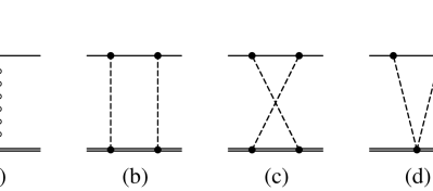
Figure 1: Contributions to energy levels of hydrogenlike ions at order $m^{2}(Z\alpha)^{2}/M$. Initial and final wavefunctions are implicit. Vertices on the top (electron) line are the usual spin-1/2 QED factors $-ie\gamma_{\mu}$ (where $e=|e|$). Vertices on the bottom (nucleus) line are those appropriate for spin-0 QED: $iZe(p+p^{\prime})_{\mu}$ for the one-photon vertex and $2i(Ze)^{2}g_{\mu\nu}$ for the seagull vertex. Part (a) represents the exchange of a transverse photon; (b) represents the exchange of two Coulomb ladder photons; (c) represents the Coulomb-Coulomb crossed ladder; and (d) represents the Coulomb-Coulomb seagull.

III.1 One-transverse photon exchange

The transverse photon propagator with momentum $q$ depends on both $q_{0}$ and $\vec{q}$. It simplifies in our formalism, which forces $q_{0}=0$, and $K_{1T}$ gives the energy shift

$$\Delta E_{1T}=-{4\pi Z\alpha\over 2\tilde{M}}\int{d^{3}k\,d^{3}l\over(2\pi)^{6}}{1\over(\vec{q}\,^{2})^{2}}[\vec{q}\,^{2}\psi^{\dagger}(\vec{k}\,)\vec{\alpha}\cdot(\vec{k}+\vec{l}\,)\psi(\vec{l}\,)-\vec{q}\cdot(\vec{k}+\vec{l}\,)\psi^{\dagger}(\vec{k}\,)\vec{\alpha}\cdot\vec{q}\psi(\vec{l}\,)],$$ (27)

where $\vec{q}=\vec{k}-\vec{l}$. If we approximate the Dirac wave functions in terms of Schrödinger wave functions through

$$\psi(\vec{p}\,)=\left(\begin{array}[]{c}\phi_{NR}(p)\chi_{\kappa\mu}(\hat{p})\\ {\vec{\sigma}\cdot\vec{p}\over 2\mu}\phi_{NR}(p)\chi_{\kappa\mu}(\hat{p})\end{array}\right),$$ (28)

this simplifies to

$$\Delta E_{1T}(NR) = -{4\pi Z\alpha\over 4m\tilde{M}}\int\frac{d^{3}k}{(2\pi)^{3}}\int\frac{d^{3}l}{(2\pi)^{3}}\,\phi^{\dagger}_{NR}(k)\phi_{NR}(l)~{}\left[{|\vec{k}+\vec{l}\,|^{2}+2i\vec{\sigma}\cdot(\vec{k}\times\vec{l}\,)\over q^{2}}-{(k^{2}-l^{2})^{2}\over q^{4}}\right]$$ (29)

$$= -{4\pi Z\alpha\over m\tilde{M}}\int\frac{d^{3}k}{(2\pi)^{3}}\int\frac{d^{3}l}{(2\pi)^{3}}\,\phi^{\dagger}_{NR}(k)\phi_{NR}(l)~{}\left[{k^{2}l^{2}-(\vec{k}\cdot\vec{l}\,)^{2}\over q^{4}}+{i\sigma\cdot(\vec{k}\times\vec{l}\,)\over 2q^{2}}\right],$$

where the spherical spinors are understood. This can be Fourier transformed into coordinate space, leading to spin independent and spin dependent operators $H_{R}$ and $H_{SO}$,

$$H_{R} = -\frac{Z\alpha}{2\mu^{2}r}\left(\delta_{ij}+\hat{x}_{i}\hat{x}_{j}\right)p_{i}p_{j}$$ (30)

$$H_{SO} = \frac{Z\alpha}{4\mu^{2}r^{3}}\vec{L}\cdot\vec{\sigma}\,.$$ (31)

After working out the expectation value of $H_{R}$ one finds

$$\Delta E_{T}=\frac{m}{M}m(Z\alpha)^{4}\left\{\frac{1}{n^{4}}+\frac{\delta_{\ell,0}}{n^{3}}-\frac{3}{n^{3}(2\ell+1)}\right\}+\frac{m}{M}<2H_{SO}>\,,$$ (32)

where

$$<H_{SO}>={\mu(Z\alpha)^{4}(j(j+1)-\ell(\ell+1)-3/4)\over 2n^{3}\ell(\ell+1)(2\ell+1)}.$$ (33)

It is of course straightforward to simply use exact wavefunctions and evaluate the integral (27) numerically. The results of doing this for the ground state using the adaptive multidimensional integration program VEGAS VEGAS are shown in Fig. 2, where the exact result is compared with the NR approximation. As is also typical for the nonrecoil case, significant differences that would be poorly treated with an expansion in $Z\alpha$ arise at high $Z$. We note that a fit can be carried out, giving

$$\Delta E_{1T}(1s)={m^{2}(Z\alpha)^{4}\over\tilde{M}}\left[-1-1.50(1)(Z\alpha)^{2}+...\right]$$ (34)

consistent with the known $(Z\alpha)^{6}$ behavior.

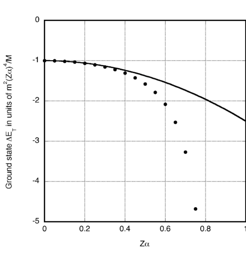
Figure 2: Plot of $\Delta E_{T}$ for the ground state as a function of $Z\alpha$ in units of $m^{2}(Z\alpha)^{4}/M$. The data points represent the result of a numerical evaluation of (27) without approximation. The solid curve is the function $-1-(3/2)(Z\alpha)^{2}$, which includes the first relativistic correction. We note that the expansion in $Z\alpha$ works well for small values of $Z$ but fails badly for large $Z$.

III.2 Coulomb-Coulomb ladder

The diagram which requires the greatest care is the two-Coulomb photon ladder diagram, as it has a binding singularity. In addition, a new feature, present in a number of loop diagrams when the nucleus is treated as a scalar, is poor convergence in the integration over the fourth component of momentum, $q_{0}$, when Coulomb photons are present. Coulomb photon propagators, being independent of $q_{0}$, provide no convergence, and the remaining $q_{0}$ is nominally logarithmically divergent, though that divergence vanishes by symmetry. We regulate this near divergence by introducing a factor $\Lambda^{2}/(q_{0}^{2}+\Lambda^{2})$ and subsequently taking $\Lambda$ to infinity. This procedure introduces a term that will be shown to cancel when a gauge invariant set of graphs is considered. Including this factor into the diagram of Fig. 1b gives the energy shift

$$\Delta E_{CC}=i{(4\pi Z\alpha)^{2}\over 2\tilde{M}}\int{d^{4}q\over(2\pi)^{4}}\int{d^{3}k\,d^{3}l\over(2\pi)^{6}}{(2\tilde{M}-q_{0})^{2}\over(\tilde{M}-q_{0})^{2}-\vec{q}\,^{2}-M^{2}+i\delta}$$

$${\Lambda^{2}\over\Lambda^{2}+q_{0}^{2}}{1\over|\vec{k}-\vec{q}\,|^{2}|\vec{q}-\vec{l}\,|^{2}}{\bar{\psi}(\vec{k}\,)\gamma_{0}[({\cal E}+q_{0})\gamma_{0}-\vec{\gamma}\cdot\vec{q}+m]\gamma_{0}\psi(\vec{l}\,)\over(({\cal E}+q_{0})^{2}-\vec{q}\,^{2}-m^{2}+i\delta)}.$$ (35)

The Dirac equation can be used to carry out the $\vec{k}$ and $\vec{l}$ integrations, leaving

$$\Delta E_{CC}={i\over 2\tilde{M}}\int{d^{4}q\over(2\pi)^{4}}{(2\tilde{M}-q_{0})^{2}\over(\tilde{M}-q_{0})^{2}-\Omega_{q}^{2}+i\delta}{\Lambda^{2}\over\Lambda^{2}+q_{0}^{2}}$$

$${\bar{\psi}(\vec{q}\,)({\cal E}\gamma_{0}-\vec{\gamma}\cdot\vec{q}-\mu)[({\cal E}+q_{0})\gamma_{0}-\vec{\gamma}\cdot\vec{q}+m]({\cal E}\gamma_{0}-\vec{\gamma}\cdot\vec{q}-\mu)\psi(\vec{q}\,)\over(({\cal E}+q_{0})^{2}-\omega_{q}^{2}+i\delta)},$$ (36)

where $\Omega_{q}=\sqrt{\vec{q}\,^{2}+M^{2}}$ and $\omega_{q}=\sqrt{\vec{q}\,^{2}+m^{2}}$. We note the ‘mismatch’ in the numerator between terms with $\mu$ and with $m$: the former come from the formalism, and the latter from the electron propagator in the diagram, which is not altered by the choice of formalism. We now carry out the $q_{0}$ integration by closing above with Cauchy’s theorem: once this is done we are free to introduce a new four-vector $q=({\cal E},\vec{q}\,)$. Three terms result, with the simplest arising from the regulator,

$$\Delta E_{CC1}={1\over 4\tilde{M}}\int\frac{d^{3}q}{(2\pi)^{3}}\bar{\psi}(\vec{q}\,)(\not\!q-\mu)\gamma_{0}(\not\!q-\mu)\psi(\vec{q}\,).$$ (37)

This term contributes in order $m^{2}(Z\alpha)^{4}/M$, but as it will be shown to cancel we do not evaluate it explicitly. The other two terms are both non-recoil, with the most sensitive being

$$\Delta E_{CC2} = {1\over 2\tilde{M}}\int\frac{d^{3}q}{(2\pi)^{3}}(\tilde{M}+\Omega_{q})^{2}{1\over 2\Omega_{q}}$$ (38)

$${\bar{\psi}(\vec{q}\,)(\not\!q-\mu)[({\cal E}+\tilde{M}-\Omega_{q})\gamma_{0}-\vec{\gamma}\cdot\vec{q}+m](\not\!q-\mu)\psi(\vec{q}\,)\over({\cal E}+\tilde{M}-\Omega_{q})^{2}-\omega_{q}^{2}}.$$

If we use the fact that

$$\frac{(\tilde{M}+\Omega_{q})^{2}}{(2\tilde{M})(2\Omega_{q})}=1+O(1/M^{2})\,$$ (39)

this simplifies to

$$\Delta E_{CC2}=\int\frac{d^{3}q}{(2\pi)^{3}}{\bar{\psi}(\vec{q}\,)(\not\!q-\mu)[({\cal E}+\tilde{M}-\Omega_{q})\gamma_{0}-\vec{\gamma}\cdot\vec{q}+m](\not\!q-\mu)\psi(\vec{q}\,)\over({\cal E}+\tilde{M}-\Omega_{q})^{2}-\omega_{q}^{2}}.$$ (40)

We proceed by rearranging the interior numerator in the above as follows:

$$\gamma^{0}({\cal E}+\tilde{M}-\Omega_{q})-\vec{\gamma}\cdot\vec{q}+m = (\not\!q+\mu)+\gamma^{0}(\tilde{M}-\Omega_{q})+(m-\mu)$$ (41)

$$= (\not\!q+\mu)+\frac{m}{M}\biggl{\{}\gamma^{0}\left(m-{\vec{q}\,^{2}\over 2m}\right)+m\biggr{\}}$$ (42)

$$= (\not\!q+\mu)+\frac{m}{M}\biggl{\{}\gamma^{0}{\cal E}+\gamma^{0}(m-{\cal E})+m-\gamma^{0}{\vec{q}\,^{2}\over 2m}\biggr{\}}$$ (43)

$$= (\not\!q+\mu)+\frac{m}{M}\biggl{\{}(\not\!q+\mu)+\gamma^{0}(m-{\cal E})$$ (45)

$$+\vec{\gamma}\cdot\vec{q}-\gamma^{0}{\vec{q}\,^{2}\over 2m}\biggr{\}}\,,$$

where in the last manipulation we have replaced $m$ with $\mu$, with the difference being higher order in $1/M$. If we now define $\kappa=q^{2}-\mu^{2}$ and restore the factors $\not\!q-\mu$ on the left and right of the interior numerator we get

$$\kappa\left(1+{m\over M}\right)(\not\!q-\mu)+{m\over M}(\not\!q-\mu)\left[\gamma^{0}(m-{\cal E})+\vec{\gamma}\cdot\vec{q}-\gamma^{0}{\vec{q}\,^{2}\over 2m}\right]\,(\not\!q-\mu).$$ (46)

We further make the expansion of the denominator

$$\bigl{(}{\cal E}+\tilde{M}-\Omega_{q}\bigr{)}^{2}-\omega_{q}^{2} = \bigl{(}{\cal E}^{2}-\vec{q}\,^{2}-\mu^{2}\bigr{)}+2{\cal E}(\tilde{M}-\Omega_{q})-(m^{2}-\mu^{2})+O(1/M^{2})$$ (47)

$$= \kappa+\frac{{\cal E}}{M}\bigl{(}2m^{2}-\vec{q}\,^{2})-2m^{3}/M+O(1/M^{2})$$ (48)

$$= \kappa+\frac{1}{M}\left\{{\cal E}({\cal E}^{2}-\vec{q}\,^{2}-m^{2})-{\cal E}^{3}+3{\cal E}m^{2}-2m^{3}\right\}+\cdots$$ (49)

$$= \kappa+\frac{1}{M}\left\{{\cal E}\kappa-(m-{\cal E})^{2}(2m+{\cal E})+\cdots\right\}$$ (50)

$$= \kappa\left[1+\frac{{\cal E}}{M}-\frac{(m-{\cal E})^{2}(2m+{\cal E})}{M\kappa}+\cdots\right]\,.$$ (51)

Combining these two forms then gives

$$\Delta E_{CC2} = \int\frac{d^{3}q}{(2\pi)^{3}}\bar{\psi}(\vec{q}\,)(\not\!q-\mu)\bigg{\{}1+\frac{(m-{\cal E})}{M}+\frac{(m-{\cal E})^{2}(2m+{\cal E})}{M\kappa}$$ (53)

$$+\frac{m}{M\kappa}\left(\gamma^{0}(m-{\cal E})+\vec{\gamma}\cdot\vec{q}-\gamma^{0}\frac{\vec{q}\,^{2}}{2m}\right)(\not\!q-\mu)\bigg{\}}\psi(\vec{q}\,)\,.$$

If we label the terms in the curly brackets in (53) parts 1-6, the various contributions are

$$\Delta E_{CC21}=<V>_{\rm Dirac}\,,$$ (54)

$$\Delta E_{CC22}=\frac{m}{M}m(Z\alpha)^{4}\biggl{\{}\frac{-1}{2n^{4}}\biggr{\}}\,,$$ (55)

$$\Delta E_{CC23}=\frac{m}{M}m(Z\alpha)^{4}\biggl{\{}\frac{3}{8n^{4}}\biggr{\}}\,,$$ (56)

$$\Delta E_{CC24}=\frac{m}{M}m(Z\alpha)^{4}\biggl{\{}\frac{-1}{4n^{4}}\biggr{\}}\,,$$ (57)

$$\Delta E_{CC25}=\frac{m}{M}m(Z\alpha)^{4}\biggl{\{}\frac{-1}{2n^{4}}+\frac{2}{n^{3}(2\ell+1)}-\frac{\delta_{\ell,0}}{n^{3}}\biggr{\}}-\frac{m}{M}<2H_{SO}>\,,$$ (58)

$$\Delta E_{CC26}=\frac{m}{M}m(Z\alpha)^{4}\biggl{\{}\frac{-1}{4n^{4}}+\frac{1}{n^{3}(2\ell+1)}\biggr{\}}\,.$$ (59)

To cancel the factor of $\kappa$ in the denominator, we note that its nonrelativistic limit is $-\vec{q}\,^{2}-(\mu Z\alpha)^{2}/n^{2}$, so that the Schrödinger equation reads

$${-\kappa\over 2\mu}\phi_{NR}(\vec{q}\,)=4\pi Z\alpha\int\frac{d^{3}p}{(2\pi)^{3}}{1\over|\vec{q}-\vec{p}\,|^{2}}\phi_{NR}(\vec{p}\,).$$ (60)

The strategy for the last three terms is then to ‘undo’ the Dirac equation so that the Coulomb potential is explicitly present, take the nonrelativistic limit as in Eq. (28), and then use the Schrödinger equation. We illustrate this with $\Delta E_{CC25}$,

$$\Delta E_{CC25} = \int\frac{d^{3}q}{(2\pi)^{3}}\frac{m}{M\kappa}\bar{\psi}(\vec{q}\,)(\not\!q-\mu)\vec{\gamma}\cdot\vec{q}\,(\not\!q-\mu)\psi(\vec{q}\,)\,$$ (61)

$$= {(4\pi Z\alpha)^{2}\over(2\pi)^{9}}\int{d^{3}k\,d^{3}q\,d^{3}l\over|\vec{k}-\vec{q}\,|^{2}|\vec{q}-\vec{l}\,|^{2}}\frac{m}{M\kappa}\bar{\psi}(\vec{k}\,)\gamma_{0}\vec{\gamma}\cdot\vec{q}\gamma_{0}\psi(\vec{l}\,)\,$$

$$\approx -{(4\pi Z\alpha)^{2}\over(2\pi)^{9}}\int{d^{3}k\,d^{3}q\,d^{3}l\over|\vec{k}-\vec{q}\,|^{2}|\vec{q}-\vec{l}\,|^{2}}\frac{m}{2M\kappa}{\phi^{\dagger}}_{NR}(\vec{k}\,)(\vec{\sigma}\cdot\vec{q}\,\vec{\sigma}\cdot\vec{l}+\vec{\sigma}\cdot\vec{k}\,\vec{\sigma}\cdot\vec{q}\,)\phi_{NR}(\vec{l}\,)\,$$

$$\approx {4\pi Z\alpha\over(2\pi)^{6}}\int{d^{3}q\,d^{3}l\over|\vec{q}-\vec{l}\,|^{2}}\frac{1}{2mM}{\phi^{\dagger}}_{NR}(\vec{q}\,)\left(\vec{q}\cdot\vec{l}+i\vec{\sigma}\cdot(\vec{q}\times\vec{l}\,)\right)\phi_{NR}(\vec{l}\,).$$

The total contribution of term $CC2$ is then

$$\Delta E_{CC2}=<V>_{\rm Dirac}+\frac{m}{M}m(Z\alpha)^{4}\biggl{\{}\frac{-9}{8n^{4}}-\frac{\delta_{\ell,0}}{n^{3}}+\frac{3}{n^{3}(2\ell+1)}\biggr{\}}-\frac{m}{M}<2H_{SO}>\,,$$ (62)

where the formalism subtracts off the first, non-recoil term. It is of interest that had we used the formalism with ${\cal E}\rightarrow\epsilon$, $\tilde{M}\rightarrow M$ mentioned above, the cancellation, while still removing the nonrecoil term, would leave a contribution that can be shown to start with the term ${m^{2}(Z\alpha)^{2}\over 2Mn^{2}}$, the standard reduced mass contribution to the nonrelativistic energy. As we have chosen to build this into our lowest order solution, the cancellation is finer, and leaves terms starting in order $m^{2}(Z\alpha)^{4}/M$.

The remaining part of the CC calculation involves closing around a negative energy electron pole, which while leading to higher powers of $Z\alpha$ than when the nuclear pole is encircled, is also nonrecoil. Its full contribution is

$$\Delta E_{CC3}={1\over 2\tilde{M}}\int{d^{3}q\over(2\pi)^{3}2\omega_{q}}(2\tilde{M}+{\cal E}+\omega_{q})^{2}{\bar{\psi}(\vec{q}\,)(\not\!q-\mu)[-\omega_{q}\gamma_{0}-\vec{\gamma}\cdot\vec{q}+m](\not\!q-\mu)\psi(\vec{q}\,)\over({\cal E}+\tilde{M}+\omega_{q})^{2}-\Omega_{q}^{2}},$$ (63)

but we can approximate ${\cal E}=m$, $\omega_{q}=m$, and $\Omega_{q}=M$ in the nuclear propagator, leading to the simpler expression

$$\Delta E_{CC3}={1\over 2\tilde{M}}\int{d^{3}q\over(2\pi)^{3}2\omega_{q}}\frac{(2\tilde{M}+2m)^{2}}{(\tilde{M}+2m)^{2}-M^{2}}\bar{\psi}(\vec{q}\,)(\not\!q-\mu)[-\omega_{q}\gamma_{0}-\vec{\gamma}\cdot\vec{q}+m](\not\!q-\mu)\psi(\vec{q}\,)\,.$$ (64)

We will show below that although this term is nonrecoil, starting in order $m(Z\alpha)^{4}$, the nonrecoil part cancels with a contribution from the crossed Coulomb ladder.

III.3 Crossed Coulomb diagram

The crossed ladder (CCX) diagram of Fig. 1c is given by

$$\Delta E_{CCX}=i{(4\pi Z\alpha)^{2}\over 2\tilde{M}}\int{d^{4}q\over(2\pi)^{4}}\int{d^{3}k\,d^{3}l\over(2\pi)^{6}}{(2\tilde{M}+q_{0})^{2}\over(\tilde{M}+q_{0})^{2}-|\vec{q}-\vec{k}-\vec{l}\,|^{2}-M^{2}+i\delta}$$

$${\Lambda^{2}\over q_{0}^{2}+\Lambda^{2}}{1\over|\vec{k}-\vec{q}\,|^{2}|\vec{q}-\vec{l}\,|^{2}}{\bar{\psi}(\vec{k}\,)\gamma_{0}[({\cal E}+q_{0})\gamma_{0}-\vec{\gamma}\cdot\vec{q}+m]\gamma_{0}\psi(\vec{l}\,)\over(({\cal E}+q_{0})^{2}-\omega_{q}^{2}+i\delta)}.$$ (65)

Taking a pole of the regulator term gives the same result as with the ladder, thus doubling $\Delta E_{CC1}$. While the pole from the nuclear line enters in the entirely negligible order $m^{5}/M^{4}$, the electron pole contributes at the level of non-recoil fine structure, and is

$$\Delta E_{CCX}={(4\pi Z\alpha)^{2}\over 2\tilde{M}}\int\frac{d^{3}q}{(2\pi)^{3}}\int{d^{3}k\,d^{3}l\over(2\pi)^{6}}{(2\tilde{M}-{\cal E}-\omega_{q})^{2}\over(\tilde{M}-{\cal E}-\omega_{q})^{2}-|\vec{q}-\vec{k}-\vec{l}\,|^{2}-M^{2}}$$

$${1\over 2\omega_{q}}{1\over|\vec{k}-\vec{q}\,|^{2}|\vec{q}-\vec{l}\,|^{2}}\bar{\psi}(\vec{k}\,)\gamma_{0}[-\omega_{q}\gamma_{0}-\vec{\gamma}\cdot\vec{q}+m]\gamma_{0}\psi(\vec{l}\,).$$ (66)

It is again legitimate to make the approximations ${\cal E}=m$, $\omega_{q}=m$, and $M^{2}+|\vec{q}-\vec{k}-\vec{l}\,|^{2}=M^{2}$, and further use of the Dirac equation gives the approximation

$$\Delta E_{CCX}={1\over 2\tilde{M}}\int{d^{3}q\over(2\pi)^{3}2\omega_{q}}{(2\tilde{M}-2m)^{2}\over(\tilde{M}-2m)^{2}-M^{2}}\bar{\psi}(\vec{q}\,)(\not\!q-\mu)[-\omega_{q}\gamma_{0}-\vec{\gamma}\cdot\vec{q}+m](\not\!q-\mu)\psi(\vec{q}\,).$$ (67)

This term can now be combined with the CC3 contribution, and the nonrecoil term can easily be seen to cancel. There remains a nonvanishing recoil term of order $m^{2}(Z\alpha)^{5}/M$,

$$\Delta E_{CC3}+\Delta E_{CCX}={1\over 2\tilde{M}}\int{d^{3}q\over(2\pi)^{3}2\omega_{q}}\bar{\psi}(\vec{q}\,)(\not\!q-\mu)[-\omega_{q}\gamma_{0}-\vec{\gamma}\cdot\vec{q}+m](\not\!q-\mu)\psi(\vec{q}\,),$$ (68)

which we keep, although beyond the order of interest we are considering here, as it has an interesting connection with the seagull diagram.

III.4 Seagull diagram

A novel feature of our formalism is the presence of so-called seagull graphs. In Coulomb gauge the seagull graph consists of a Coulomb-Coulomb (CC) term and a transverse-transverse term (TT), with the latter beyond our present order of interest. Again regularizing the $q_{0}$ integration, the CC seagull graph (see Fig. 1d) contributes

$$\Delta E_{CCs} = -2i{(4\pi Z\alpha)^{2}\over 2\tilde{M}}\int{d^{4}q\over(2\pi)^{4}}\int{d^{3}k\,d^{3}l\over(2\pi)^{6}}{\Lambda^{2}\over\Lambda^{2}+q_{0}^{2}}$$ (69)

$${1\over|\vec{k}-\vec{q}\,|^{2}|\vec{q}-\vec{l}\,|^{2}}{\bar{\psi}(\vec{k}\,)\gamma_{0}[({\cal E}+q_{0})\gamma_{0}-\vec{\gamma}\cdot\vec{q}+m]\gamma_{0}\psi(\vec{l}\,)\over(({\cal E}+q_{0})^{2}-\vec{q}\,^{2}-m^{2}+i\delta)}.$$

If we again close above to carry out the $q_{0}$ integration the regulator term contributes $-2\Delta E_{CC1}$: as $\Delta E_{CC1}$ was doubled from the crossed Coulomb diagram, this completes the cancellation of contributions arising from the regulator term. The other pole picks up a negative energy electron contribution, and gives, using the Dirac equation,

$$\Delta E_{CCs}=-2{1\over 2\tilde{M}}\int{d^{3}q\over(2\pi)^{3}2\omega_{q}}\bar{\psi}(\vec{q}\,)(\not\!q-\mu)[-\omega_{q}\gamma_{0}-\vec{\gamma}\cdot\vec{q}+m](\not\!q-\mu)\psi(\vec{q}\,).$$ (70)

The net result is that the only role of the seagull diagram to order $m^{2}(Z\alpha)^{4}/M$ is in canceling the regulator terms from the ladder and crossed ladder, and in addition it combines with $m^{2}(Z\alpha)^{5}/M$ terms coming from the negative energy pole terms in those diagrams.

IV Total at order $(Z\alpha)^{4}$

The combination of the CC, CCX, CCs, T, and -C graphs gives

$$\Delta E=\frac{m}{M}m(Z\alpha)^{4}\left\{\frac{-1}{8n^{4}}\right\}\,.$$ (71)

In order to find the total recoil contribution at this order, one must combine this with the recoil contribution from $\mu(f(n,j)-1)$, which is $-(m^{2}/M)(f(n,j)-1)$ where $f(n,j)=\epsilon/m$ is defined through Eq. (5). The total recoil contribution through terms of order $(Z\alpha)^{4}$ is

$$\Delta E_{\rm recoil} = \frac{m^{2}}{M}\biggl{\{}-\bigl{(}f(n,j)-1\bigr{)}-\frac{(Z\alpha)^{4}}{8n^{4}}\biggr{\}}$$ (72)

$$= \frac{m^{2}}{M}\biggl{\{}\frac{(Z\alpha)^{2}}{2n^{2}}+(Z\alpha)^{4}\biggl{(}\frac{-1}{2n^{4}}+\frac{1}{2n^{3}(j+1/2)}\biggr{)}\biggr{\}}\,.$$ (73)

This is the known Barker and Glover result Barker for the recoil contribution at this order.

V Salpeter correction

One of the first accomplishments of a fully relativistic treatment of the two-body bound state problem was Salpeter’s discovery Salpeter that corrections of order $\alpha m/M$ times fine structure were present in hydrogenlike atoms: use of the older formalism of the Breit equation had found no such contributions Arfken . While we are not calculating all such terms here, we show how they arise from one and higher Coulomb exchanges that are crossed by a transverse photon, illustrating with the graph of Fig. 3a. This gives rise to the somewhat complicated expression

$$\Delta E = -{(4\pi Z\alpha)^{3}\over 2M}\int{d^{4}k\over(2\pi)^{4}}\int{d^{4}l\over(2\pi)^{4}}\int{d^{3}p\,d^{3}p^{\prime}\over(2\pi)^{6}}{(2M+2k_{0}-l_{0})\over(M+k_{0})^{2}-|\vec{k}-\vec{p}\,|^{2}-M^{2}+i\delta}$$ (74)

$${(2M+k_{0}-l_{0})\over[(M+k_{0}-l_{0})^{2}-|\vec{k}-\vec{l}\,|^{2}-M^{2}+i\delta]}{(k-2p)_{j}(\delta_{ij}-{k_{i}k_{j}\over\vec{k}^{2}})\over k_{0}^{2}-\vec{k}^{2}+i\delta}{1\over|\vec{l}-\vec{p}\,|^{2}}{1\over|\vec{k}-\vec{l}+\vec{p}\,^{\prime}|^{2}}$$

$$\bar{\psi}(\vec{p}\,^{\prime})\gamma_{i}{1\over({\cal E}+k_{0})\gamma_{0}-\vec{\gamma}\cdot(\vec{k}+\vec{p}\,^{\prime})-m+i\delta}\gamma_{0}{1\over({\cal E}+l_{0})\gamma_{0}-\vec{\gamma}\cdot\vec{l}-m+i\delta}\gamma_{0}\psi(\vec{p}\,).$$

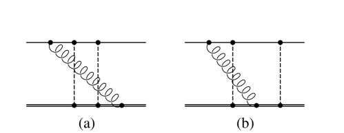
Figure 3: Graphs contributing to the Salpeter correction of order $m^{2}(Z\alpha)^{5}/M$. In graph (a) a transverse photon crosses two Coulomb photons. In graph (b) the transverse photon crosses a single Coulomb photon, with a Coulomb ladder photon on the side. There are two graphs like (b) since the ladder photon can be on either side.

We wish to show that this expression is dominated by a term that contains part of the Dirac-Coulomb propagator of Eq. (2). Specifically, if we expand the momentum space form of that equation in powers of the Coulomb potential, the term involving one potential is

$$S_{F}^{1C}(\vec{p},\vec{p}\,^{\prime};E)={1\over E\gamma_{0}-\vec{\gamma}\cdot\vec{p}\,^{\prime}-m}{-4\pi Z\alpha\over|\vec{p}\,^{\prime}-\vec{p}\,|^{2}}\gamma_{0}{1\over E\gamma_{0}-\vec{\gamma}\cdot\vec{p}-m},$$ (75)

where the distinction between $m$ and $\mu$ is dropped in this section as the graph being considered has a factor $m/M$. To see how this arises from the graph of Fig. 3a, we first close the $k_{0}$ contour above and take the transverse photon pole to get

$$\Delta E = i{(4\pi Z\alpha)^{3}\over 4M}\int{d^{3}k\over(2\pi)^{3}}{1\over k}\int{d^{4}l\over(2\pi)^{4}}\int{d^{3}p\,d^{3}p^{\prime}\over(2\pi)^{6}}{(2M-2k-l_{0})\over(M-k)^{2}-|\vec{k}-\vec{p}\,|^{2}-M^{2}}$$ (76)

$${(2M-k-l_{0})\over[(M-k-l_{0})^{2}-|\vec{k}-\vec{l}\,|^{2}-M^{2}+i\delta]}(-2p)_{j}\left(\delta_{ij}-{k_{i}k_{j}\over\vec{k}^{2}}\right){1\over|\vec{l}-\vec{p}\,|^{2}}{1\over|\vec{k}-\vec{l}+\vec{p}\,^{\prime}|^{2}}$$

$$\bar{\psi}(\vec{p}\,^{\prime})\gamma_{i}{1\over({\cal E}-k)\gamma_{0}-\vec{\gamma}\cdot(\vec{k}+\vec{p}\,^{\prime})-m}\gamma_{0}{1\over({\cal E}+l_{0})\gamma_{0}-\vec{\gamma}\cdot\vec{l}-m+i\delta}\gamma_{0}\psi(\vec{p}\,).$$

Because we are dropping terms of order $m^{3}/M^{2}$, the first nuclear denominator simplifies to $-2Mk$, and further carrying out the $l_{0}$ integration by closing above gives a term from the second nuclear denominator that forces $l_{0}=-k$, giving

$$\Delta E = -{(4\pi Z\alpha)^{3}\over 4M}\int{d^{3}k\over(2\pi)^{3}}{1\over k^{2}}\int{d^{3}l\over(2\pi)^{3}}\int{d^{3}p\,d^{3}p^{\prime}\over(2\pi)^{6}}(-2p)_{j}\left(\delta_{ij}-{k_{i}k_{j}\over\vec{k}^{2}}\right){1\over|\vec{l}-\vec{p}\,|^{2}}{1\over|\vec{k}-\vec{l}+\vec{p}\,^{\prime}|^{2}}$$ (77)

$$\bar{\psi}(\vec{p}\,^{\prime})\gamma_{i}{1\over({\cal E}-k)\gamma_{0}-\vec{\gamma}\cdot(\vec{k}+\vec{p}\,^{\prime})-m}\gamma_{0}{1\over({\cal E}-k)\gamma_{0}-\vec{\gamma}\cdot\vec{l}-m}\gamma_{0}\psi(\vec{p}\,).$$

The Salpeter correction is associated with the region of integration in which $k\sim m(Z\alpha)^{2}$ rather than the normal $m(Z\alpha)$. In this region one can approximate $\vec{k}+\vec{p}\,^{\prime}=\vec{p}\,^{\prime}$ and $\vec{k}-\vec{l}+\vec{p}\,^{\prime}=-\vec{l}+\vec{p}\,^{\prime}$ in the above. Using Eq. (75) then allows us to write

$$\Delta E = \frac{(4\pi Z\alpha)^{2}}{4M}\int{d^{3}k\over(2\pi)^{3}}{1\over k^{2}}\int{d^{3}l\over(2\pi)^{3}}\int{d^{3}p\,d^{3}p^{\prime}\over(2\pi)^{6}}(-2p)_{j}\left(\delta_{ij}-{k_{i}k_{j}\over\vec{k}^{2}}\right){1\over|\vec{l}-\vec{p}\,|^{2}}$$ (78)

$$\bar{\psi}(\vec{p}\,^{\prime})\gamma_{i}S_{F}^{1C}(\vec{p}\,^{\prime},\vec{l};{\cal E}-k)\gamma_{0}\psi(\vec{p}\,).$$

The same kinds of argument apply for any number of Coulomb exchanges, allowing the replacement of $S_{F}^{1C}$ with $S_{F}$. Care is required, however, for the first term of the expansion of $S_{F}$, which requires an ultraviolet cutoff in the $k$ integration because of the approximations we have made. However, this term is finite when simply treated as a one loop diagram. The actual calculation of the Salpeter correction would involve evaluating the one loop diagram without approximation and then evaluating the above expression and higher Coulomb exchanges by using $S_{F}-S_{0}$, a technique that is standard in self-energy calculations. Replacing $S_{F}^{1C}$ in the above with the spectral representation of $S_{F}$ then gives

$$\Delta E = \frac{(4\pi Z\alpha)^{2}}{4M}\int{d^{3}k\over(2\pi)^{3}}{1\over k^{2}}\int{d^{3}l\over(2\pi)^{3}}\int{d^{3}p\,d^{3}p^{\prime}\over(2\pi)^{6}}(-2p)_{j}\left(\delta_{ij}-{k_{i}k_{j}\over\vec{k}^{2}}\right){1\over|\vec{l}-\vec{p}\,|^{2}}$$ (79)

$$\sum_{m}{\bar{\psi}(\vec{p}\,^{\prime})\gamma_{i}\psi_{m}(\vec{p}\,^{\prime})\bar{\psi}_{m}(\vec{l}\,)\gamma_{0}\psi(\vec{p}\,)\over{\cal E}-E_{m}-k}.$$

Replacing $-2p_{j}$ with $-2(p-l)_{j}$ leads to the integral

$$\int{d^{3}p\,d^{3}l\over(2\pi)^{6}}(p-l)_{j}{{4\pi Z\alpha}\over|\vec{l}-\vec{p}\,|^{2}}\bar{\psi}_{m}(\vec{l}\,)\gamma_{0}\psi(\vec{p}\,)$$ (80)

$$= -iZ\alpha\int d^{3}x{x_{j}\over x^{3}}\bar{\psi}_{m}(\vec{x}\,)\gamma_{0}\psi(\vec{x}\,)$$

$$= ({\cal E}-E_{m})<m|p_{j}|0>$$

where $\cal E$ is the Dirac energy of the state $\psi$ of interest, here taken to be the ground state. Eqs. (79) and (80) lead to the relativistic generalization of Salpeter’s Salpeter Eq. (45). The replacement of $-2p_{j}$ by $-2(p-l)_{j}$ arises from consideration of the reducible graph shown in Fig. 3b, which comes from the formalism when three-photon exchange is considered, as described in Ref. poshfs . In this diagram there are two nuclear propagators that depend on $l_{0}$, with one of them leading to the replacement mentioned above, and the other to a bound state singularity canceled by the formalism.

VI NRQED calculation of the energy shift to order $(Z\alpha)^{4}$ including recoil

We base our expression of NRQED on the work of Kinoshita and Nio Kinoshita96 . The NRQED Lagrangian for a particle of spin-1/2 and one of spin-0 has the form

$${\cal L} = \psi^{\dagger}\Biggl{\{}iD_{t}+\frac{\vec{D}^{2}}{2m}+\frac{\vec{D}^{4}}{8m^{3}}+c_{F}\frac{e\vec{\sigma}\cdot\vec{B}}{2m}$$ (83)

$$+c_{D}\frac{e(\vec{D}\cdot\vec{E}-\vec{E}\cdot\vec{D})}{8m^{2}}+c_{S}\frac{ie\vec{\sigma}\cdot(\vec{D}\times\vec{E}-\vec{E}\times\vec{D})}{8m^{2}}+\cdots\Biggr{\}}\psi$$

$$+\phi\Biggl{\{}iD_{t}+\frac{\vec{D}^{2}}{2M}+\cdots\Biggr{\}}\phi+{\cal L}_{EM}\,,$$

where $D_{t}=\partial_{t}+ieA^{0}$ and $\vec{D}=\vec{\partial}-ie\vec{A}$ for the electron, and similarly but with $e\rightarrow-Ze$ for the nucleus. Electromagnetism is described by the usual Lagrangian ${\cal L}_{EM}=(-1/4)F_{\mu\nu}F^{\mu\nu}$, and we use Coulomb gauge in our calculations. In terms of Feynman rules, we build on those given by Kinoshita and Nio in their Fig. 3. The new rules include a Coulomb vertex for the nucleus $-Ze$, a dipole vertex for the nucleus $Ze(\vec{p}\,^{\prime}+\vec{p}\,)/(2M)$, and a propagator for the nucleus $(E-\vec{p}\,^{2}/(2M)+i\epsilon)^{-1}$. The rule is to multiply all propagators by $i$, all vertices by $-i$, and to include an overall factor of $i$ when calculating energy shifts. Loop integrals are done over all momenta with measure $d^{4}k/(2\pi)^{4}$. The Bethe-Salpeter equation for NRQED (with lowest order propagators and vertices) is exactly the Schrödinger-Coulomb equation with reduced mass, which is also described in Kinoshita and Nio. We use the symbol $\Psi(p)$ for the NRQED Bethe-Salpeter wave function. For example, the ground state wave function is

$$\Psi(p)=(2\pi)\delta(p_{0})\psi(\vec{p}\,)\,,$$ (84)

where

$$\psi(\vec{p}\,)=\frac{16\pi\xi^{5/2}}{(\vec{p}\,^{2}+\xi^{2})^{2}}\chi_{-1\mu}$$ (85)

with $\xi=\mu Z\alpha$ and, for example, ${\chi^{\dagger}}_{-1,\frac{1}{2}}=\frac{1}{\sqrt{4\pi}}(1,0)$.

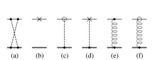
Figure 4: NRQED contributions to energies at order $m^{2}(Z\alpha)^{4}/M$. Graph (a) is the two-Coulomb crossed ladder, (b) represents the $p^{4}$ relativistic kinetic energy correction to the electron line, (c) is the spin-orbit correction to the electron line (with Coulomb photon exchange), (d) is the Darwin correction to the electron line (with Coulomb photon exchange), (e) shows transverse photon exchange with dipole vertices on both electron and nuclear lines, and (f) represents transverse photon exchange with a Fermi vertex on the electron line and a dipole vertex on the nuclear line.

The relevant graphs for the calculation of energies up to $O((Z\alpha)^{4})$ and including recoil (to first order: $m/M$) are shown in Fig. 4. In the calculation of bound state NRQED graphs we take the electron line to enter with momentum $({\cal E}_{0},\vec{p}\,)$ and the nucleus with momentum $(0,-\vec{p}\,)$ where ${\cal E}_{0}=-\mu(Z\alpha)^{2}/(2n^{2})$ is the Bohr energy level.

The crossed Coulomb ladder (Fig. 4a) has the form

$$\Delta E_{CCX} = i\int\frac{d^{3}q}{(2\pi)^{3}}\frac{d^{4}l}{(2\pi)^{4}}\frac{d^{3}p}{(2\pi)^{3}}\psi^{\dagger}(\vec{q}\,)(-ie)\frac{i}{l_{0}+{\cal E}_{0}-\frac{\vec{l}\,^{2}}{2m}+i\epsilon}(-ie)\psi(\vec{p}\,)$$ (87)

$$\times\frac{i}{(\vec{q}-\vec{l}\,)^{2}}\frac{i}{(\vec{l}-\vec{p}\,)^{2}}(iZe)\frac{i}{l_{0}-\frac{(\vec{l}-\vec{p}-\vec{q}\,)^{2}}{2M}+i\epsilon}(iZe)\,.$$

The poles of the $l_{0}$ integral

$$\int\frac{dl_{0}}{2\pi i}\frac{1}{l_{0}+{\cal E}_{0}-\frac{\vec{l}\,^{2}}{2m}+i\epsilon}\frac{1}{l_{0}-\frac{(\vec{l}-\vec{p}-\vec{q}\,)^{2}}{2m}+i\epsilon}=0.$$ (88)

are both on the same side of the real axis. It follows that the $l_{0}$ integral vanishes, as does the crossed Coulomb ladder contribution: $\Delta E_{CCX}=0$.

The relativistic kinetic energy correction (Fig. 4b) is

$$\Delta E_{K} = i\int\frac{d^{3}q\,d^{3}p}{(2\pi)^{6}}\,\psi^{\dagger}(\vec{q}\,)(-i)\left(\frac{-\vec{p}\,^{4}}{8m^{3}}\right)(2\pi)^{3}\delta(\vec{p}-\vec{q}\,)\psi(\vec{p}\,)$$ (89)

$$= \left(\frac{\mu}{m}\right)^{3}\left<H_{K}\right>$$ (90)

$$\approx \left(1-\frac{3m}{M}\right)\left<H_{K}\right>\,,$$ (91)

where

$$\left<H_{K}\right>=\int\frac{d^{3}p}{(2\pi)^{3}}\psi^{\dagger}(\vec{p}\,)\left(\frac{-\vec{p}\,^{4}}{8\mu^{3}}\right)\psi(\vec{p}\,)=\mu(Z\alpha)^{4}\left(\frac{3}{8n^{4}}-\frac{1}{(2\ell+1)n^{3}}\right)\,.$$ (92)

The spin-orbit correction to the electron line (Fig. 4c) is

$$\Delta E_{SO} = i\int\frac{d^{3}q\,d^{3}p}{(2\pi)^{6}}\,\psi^{\dagger}(\vec{q}\,)(-i)\frac{ie}{4m^{2}}\left(\vec{q}\times\vec{p}\,\right)\cdot\vec{\sigma}\psi(\vec{p}\,)\frac{i}{\vec{k}\,^{2}}(iZe)$$ (93)

$$= \frac{i}{4m^{2}}\int\frac{d^{3}q\,d^{3}p}{(2\pi)^{6}}\,\psi^{\dagger}(\vec{q}\,)\left(\vec{q}\times\vec{p}\cdot\vec{\sigma}\right)\psi(\vec{p}\,)V_{C}(\vec{k}\,)$$ (94)

$$= \left(\frac{\mu}{m}\right)^{2}\left<H_{SO}\right>$$ (95)

$$\approx \left(1-\frac{2m}{M}\right)\left<H_{SO}\right>\,,$$ (96)

where $\vec{k}=\vec{q}-\vec{p}$ and

$$\left<H_{SO}\right>=\left<\frac{Z\alpha}{4\mu^{2}r^{3}}\vec{L}\cdot\vec{\sigma}\right>$$ (97)

as before.

The Darwin correction to the electron line (Fig. 4d) is

$$\Delta E_{D} = i\int\frac{d^{3}q\,d^{3}p}{(2\pi)^{6}}\,\psi^{\dagger}(\vec{q}\,)\frac{ie}{8m^{2}}\left|\vec{q}-\vec{p}\,\right|^{2}\psi(\vec{p}\,)\frac{i}{\vec{k}\,^{2}}(iZe)$$ (98)

$$= \left(\frac{\mu}{m}\right)^{2}\frac{4\pi Z\alpha}{8\mu^{2}}\left|\psi(0)\right|^{2}$$ (99)

$$\approx \left(1-\frac{2m}{M}\right)\left<H_{D}\right>\,,$$ (100)

where

$$\left<H_{D}\right>=\frac{4\pi Z\alpha}{8\mu^{2}}\left|\psi(0)\right|^{2}=\mu(Z\alpha)^{4}\frac{\delta_{\ell,0}}{2n^{3}}\,.$$ (101)

The dipole-dipole transverse photon exchange contribution (Fig. 4e) is

$$\Delta E_{DD} = i\int\frac{d^{3}q\,d^{3}p}{(2\pi)^{6}}\,\psi^{\dagger}(\vec{q}\,)\frac{ie}{2m}(p+q)^{i}\frac{i\delta^{T}_{ij}(\vec{k}\,)}{-\vec{k}\,^{2}}\psi(\vec{p}\,)\frac{-iZe}{2M}(-p-q)^{j}$$ (102)

$$= \frac{-4\pi Z\alpha}{mM}\int\frac{d^{3}q\,d^{3}p}{(2\pi)^{6}}\,\psi^{\dagger}(\vec{q}\,)\frac{\vec{p}\,^{2}\vec{q}\,^{2}-(\vec{p}\cdot\vec{q}\,)^{2}}{\vec{k}\,^{4}}\psi(\vec{p}\,)$$ (103)

$$= \frac{m}{M}\left<H_{R}\right>\,,$$ (104)

just as in the relativistic calculation of one transverse photon exchange. We note that the expectation value $\left<H_{R}\right>$ can be written as

$$\left<H_{R}\right> = \left\{\frac{1}{n^{4}}+\frac{\delta_{\ell,0}}{n^{3}}-\frac{3}{n^{3}(2\ell+1)}\right\}\mu(Z\alpha)^{4}$$ (105)

$$= 3\left<H_{K}\right>+2\left<H_{D}\right>-\frac{1}{8n^{4}}\mu(Z\alpha)^{4}\,.$$ (106)

Finally, the Fermi correction (Fig. 4f) is

$$\Delta E_{F} = \frac{-4\pi Z\alpha}{4mM}\int\frac{d^{3}q\,d^{3}p}{(2\pi)^{6}}\,\psi^{\dagger}(\vec{q}\,)\frac{-i\epsilon_{ijk}(q-p)_{j}\sigma_{k}\delta^{T}_{in}(\vec{k}\,)(p+q)_{n}}{\vec{k}\,^{2}}\psi(\vec{p}\,)$$ (107)

$$= \frac{2i}{4mM}\int\frac{d^{3}q\,d^{3}p}{(2\pi)^{6}}\,\psi^{\dagger}(\vec{q}\,)\vec{q}\times\vec{p}\cdot\vec{\sigma}\psi(\vec{p}\,)V_{C}(\vec{k}\,)$$ (108)

$$= \frac{m}{M}\left<\frac{Z\alpha}{2m^{2}r^{3}}\vec{L}\cdot\vec{\sigma}\right>$$ (109)

$$\approx \frac{m}{M}\left<2H_{SO}\right>\,.$$ (110)

The sum of all contributions is

$$\Delta E = \Delta E_{CCX}+\Delta E_{K}+\Delta E_{SO}+\Delta E_{D}+\Delta E_{DD}+\Delta E_{F}$$ (111)

$$= \left(1-\frac{3m}{M}\right)\left<H_{K}\right>+\left(1-\frac{2m}{M}\right)\left<H_{SO}\right>+\left(1-\frac{2m}{M}\right)\left<H_{D}\right>$$ (113)

$$+\frac{m}{M}\left(3\left<H_{K}\right>+2\left<H_{D}\right>-\frac{1}{8n^{4}}\mu(Z\alpha)^{4}\right)+\frac{m}{M}\left<2H_{SO}\right>$$

$$= \left<H_{K}+H_{SO}+H_{D}\right>-\frac{m^{2}}{M}\frac{(Z\alpha)^{4}}{8n^{4}}\,,$$ (114)

which again is the known Barker and Glover result for the fine structure with recoil correction.

VII Conclusions

A form of the Bethe-Salpeter equation of particular simplicity has been introduced that can be applied to the entire hydrogen isoelectronic sequence. We have shown that the power series expansion of the 1T kernel is nonperturbative at high $Z$, demonstrating the need for a complete numerical calculation for all kernels. Such a calculation has been done using a Green’s function formalism by Shabaev and collaborators Victor , Victors , but it is always desirable in QED to have checks on these complex calculations. We are presently calculating the remaining one-loop diagrams that enter in order $m^{2}/M(Z\alpha)^{5}$. As an indication of the numerical importance of these calculations for the transition discussed in the introduction, we note that Ref. Victors finds a correction of -0.04 eV for the $2p_{1/2}-2s$ transition in hydrogenic uranium, to be compared to the 0.207 eV discrepancy presumably dominated by the two-loop Lamb shift. However, this is only part of the effect of recoil for lithiumlike uranium, and the question of relativistic corrections to mass polarization cannot be addressed in our formalism, which is strictly a two-body approach. We are presently investigating the relatively unexplored problem of forming many-particle generalizations of the Bethe-Salpeter equation that have the three-dimensional and relativistic aspects of the equation described in the present work.

- (1) See contributions in Atomic, Molecular, and Optical Physics Handbook, ed G.W.F. Drake (AIP Press, 2005).
- (2) Z.-C. Yan and G.W.F. Drake, Phys. Rev. A 66, 042504 (2002); F.W. King, Phys. Rev. A 43, 3285 (1991).
- (3) K. Pachucki and J. Komasa, Phys. Rev. Lett. 92, 213001 (2004).
- (4) W.E. Caswell and G.P. Lepage, Phys. Lett. B 167, 437 (1986).
- (5) K. Pachucki, Phys. Rev. A 56, 297 (1997).
- (6) P. Beiersdorfer, H. Chen, D.B. Thorn, and E. Träbert, Phys. Rev. Lett. 95, 233003 (2005).
- (7) W.H. Furry, Phys. Rev. 81, 115 (1951).
- (8) E.H. Wichmann and N.M. Kroll, Phys. Rev. 101, 843 (1956).
- (9) G.E. Brown, J.S. Langer, and G.W. Schaefer, Proc. Roy. Soc. London, Ser. A 251, 92 (1959).
- (10) V.A. Yerokhin, P. Indelicato, and V.M. Shabaev, Phys. Rev. Lett. 91, 073001 (2003).
- (11) V.M Shabaev, Phys. Rev. A 57, 59 (1998).
- (12) A.N. Artemyev, V.M Shabaev, and V.A. Yerokhin, Phys. Rev. A 52, 1884 (1995).
- (13) E.E. Salpeter and H.A. Bethe, Phys. Rev. 84, 1232 (1951).
- (14) E.E. Salpeter, Phys. Rev. 87, 328 (1952).
- (15) G. P. Lepage, Phys. Rev. A 16, 863 (1977).
- (16) C. Fronsdal and R. W. Huff, Phys. Rev. D 3, 933 (1971).
- (17) W.E. Caswell and G.P. Lepage, Phys. Rev. A 18, 810 (1978).
- (18) G.S. Adkins and R.N. Fell, Phys. Rev. A 60, 4461 (1999).
- (19) See Section IIC of the above reference.
- (20) W.A. Barker and F.N. Glover, Phys. Rev. 99, 317 (1955).
- (21) G. Breit and G.E. Brown, Phys. Rev. 74, 1278 (1948).
- (22) G.P. Lepage, J. Comp. Phys. 27, 192 (1978).
- (23) G.S. Adkins and J. Sapirstein, Phys. Rev. A 58, 3552 (1998).
- (24) T. Kinoshita and M. Nio, Phys. Rev. D 53, 4909 (1996).