Instanton-inspired Model of QCD Phase Transition and Bubble Dynamics

Abstract

We have reinvestigated the collision of gluonic bubbles in a SU(2) model of QCD which was studied by Johnson, Choi and Kisslinger in the context of the instanton-inspired model of QCD phase transition bubbles with plane wave approximation. We discuss treacherous points of the instanton-inspired model that cause the violation of causality due to the presence of imaginary gluon fields. By constructing a new slightly modified Lorentzian model where we have three independent real gluon fields, we reanalyzed the process of bubble collisions. Our numerical results show some indication of forming a bubble wall in colliding region.

I Introduction

With the current advances of Relativistic Heavy Ion Collider(RHIC) RHICwebsite and Cosmology in the Laboratory(COSLAB) COSLABwebsite programs, there is a growing interest in discussing the self-organizing nature common to many different physical systems. In particular, the phase transition and the defect formation are the paramount examples of the physical phenomena due to the self-organizing nature of many-body systems. In the RHIC facilities, vigorous analyses are underway to find if the evidences of forming the quark-gluon plasma indeed reveal in the experimental data by smashing the heavy ions. Also, the main emphasis of the COSLAB program is to exploit the analogies between the phase transitions in the universe at the time of the hot Big Bang and the observable transitions in the condensed matter systems at low temperatures. Consequently, the physical systems experimented in the RHIC and COSLAB programs are very diverse, spanning hadronic matter, superfluid Helium, superconductors, liquid crystals, cosmic strings, etc.. Essential theoretical tools to study these physical systems are provided by the quantum field theories (QFTs) including the quantum chromodynamics (QCD), the toy models of QCD such as Thirring model Thirring and sine-Gordon model sine-Gordon , and many other dynamical model theories describing the strongly correlated systems. The description of the above self-organizing nature with the QFTs, however, cannot rely on the ordinary perturbative approach because the strong correlations among the quanta in the formation of new phases are intrinsically nonperturbative going beyond the realm of the quantum mechanical von Neumann’s theorem vonNeumann .

Consideration of phase transitions in early universe has a rather long history col ; hms and relevant bubble dynamics has been discussed frequently in the past manyworks . Recently, the domain walls in QCD have been discussed as examples of topological defects which may play an important role in the evolution of the early universe soon after the QCD phase transition Forbes:2000et ; ae ; cst . In particular, the possibility of primordial magnetic field generation has been discussed as a consequence of the existence of QCD domain walls Forbes:2000et . Subsequently, a claim for the formation of cosmological color magnetic wall in the universe was also made by utilizing the QCD instanton solutions Kisslinger:2002py ; Kisslinger:2002mu ; Johnson:2003ti .

Due to the topological configurations of the fields, the domain walls and the instanton solutions may be stable. Thus, it has been suggested that the QCD domain walls may be detectable at RHIC facilities Forbes:2000et . In the COSLAB, reproducing black hole radiation phenomena (i.e., the so-called Hawking radiation Hawking .) in the table top experiments may be realized by the phonon radiation from a dumb hole in acoustic geometry dumbhole . Also discussed is testing various black hole solutions of the Einstein equation in the laboratory vachaspati . Similarly, the COSLAB activities COSLABwebsite may be applicable as well to study the collisions of the domain walls or the so-called bubble collisions in the laboratory.

Furthermore, the existence of these topological configurations in the universe may give an impact on our understanding of the dark matter which has been one of the biggest puzzles in the cosmology for more than a decade. Already, the QCD domain wall has been related to the axion domain wall Forbes:2000et . However, the more direct connection between the dark matter and the QCD vacuum condensates has been indicated by the recent molar mass estimate of dark matter from the strong gravitational lensing in the galaxy cluster MJ . This estimate also supported by the analyses of the universal rotation curves in spiral galaxies Persic revealed that the mass scale of the dark matter particles may be very close to the QCD scale $\Lambda_{QCD}$ MJ ; Ariel . Thus, further detailed studies of the QCD vacuum properties such as the QCD domain walls and the QCD instanton solutions hooft ; instanton are necessary to confirm any connection between the QCD vacuum and the dark matter in the universe.

Motivated by these previous works, we discuss the bubble dynamics in nonabelian Yang-Mills theory as a prototype of QCD in this work. In particular, we reanalyze the formation of cosmological color magnetic wall with and without following the previous procedure discussed by Kisslinger, et al. Kisslinger:2002py ; Kisslinger:2002mu ; Johnson:2003ti and present both the treacherous points of the previous analysis and some new progresses made in the present analysis. Although the potential existence of cosmological magnetic wall and the importance of its implication on the dark matter and cosmology are undeniable, our analysis indicates that simplified model calculations are not capable of verifying its existence and much more careful studies would be necessary to confirm the possibility.

The paper is organized as follows. In the next section (Section II), we briefly go over the equations of motion and the energy-momentum tensor in the instanton-inspired model of the QCD phase transition bubbles. In Section III, we solve the derived equations numerically in a plane-wave model describing the collision of the two bubbles in the vicinity of the contacting surface: (a) with the Wick rotation procedure followed by the previous analysis in Ref. Johnson:2003ti , (b) with our own method strictly valid in Lorentzian space. In Section III (a), we reproduce the results obtained by the previous analysis and present the error estimates of these results to discuss the treacherous points in the analysis. Moreover, we point out that the way of solving the system of equations having a constraint should be corrected from the previous analysis. By solving the constraint equation first and applying it to the dynamical one, we show that the numerical results are very different from those in Ref. Johnson:2003ti . In Section III (b), it is pointed out that the instanton-inspired model studied in Refs. Kisslinger:2002py ; Kisslinger:2002mu ; Johnson:2003ti should be modified due to the presence of imaginary gluon fields. By constructing a new slightly modified Lorentzian model, we present our own results indicating the formation of a bubble wall in colliding region. Conclusions and Discussions follow in Section IV. In the appendix, more details of error estimates are presented.

II Instanton-inspired model of QCD phase transition bubbles

During the time interval between $10^{-5}$-$10^{-4}$s when the universe passed through the critical temperature $T_{\rm c}\simeq 150$ Mev for the chiral phase transition, the quark-hadron phase transition (QHPT) occurs. If QHPT occurs as a first order phase transition, bubbles could form. Recently, a model for describing bubble collisions has been formulated in Refs. Kisslinger:2002py ; Kisslinger:2002mu ; Johnson:2003ti . Since the main structure of the bubble must be gluonic in nature, pure gluodynamics was used. In this section, we briefly review the instanton-inspired model of QCD bubble walls in Refs. Kisslinger:2002py ; Kisslinger:2002mu ; Johnson:2003ti .

The action for pure glue is

$$S=-\frac{1}{4}\int\;d^{4}xF\cdot F,$$ (1)

where

$$F_{\mu\nu}=\partial_{\mu}A_{\nu}-\partial_{\nu}A_{\mu}-ig[A_{\mu},A_{\nu}].$$ (2)

For simplicity SU(2) color gauge field can be considered;

$$A_{\mu} = A^{a}_{\mu}(\sigma^{a}/2)$$ (3)

with the Pauli matrix $\sigma_{a}$ satisfying $[\sigma^{a},\sigma^{b}]=2i\epsilon^{abc}\sigma^{c}$ and $Tr(\sigma^{a}\sigma^{b})=2\delta^{ab}$. Thus, we have

$$F^{a}_{\mu\nu}=\partial_{\mu}A^{a}_{\nu}-\partial_{\nu}A^{a}_{\mu}+g\epsilon^{abc}A^{b}_{\mu}A^{c}_{\nu},$$ (4)

and the field equations in the Lorentz gauge, $\partial^{\mu}A^{a}_{\mu}=0$, become

$$\partial_{\mu}\partial^{\mu}A^{a}_{\nu}+g\epsilon^{abc}(2A^{b}_{\mu}\partial^{\mu}A^{c}_{\nu}-A^{b}_{\mu}\partial_{\nu}A^{\mu c})+g^{2}\epsilon^{abc}\epsilon^{cef}A^{b}_{\mu}A^{\mu e}A^{f}_{\nu}=0.$$ (5)

As is well known, the Euclidean equation of Eq.(5) has an instanton solution given by

$$\tilde{A}_{\mu}^{a,{\rm inst}}(x)=\frac{2}{g}\tilde{\eta}^{a}_{\mu\nu}\frac{x^{\nu}}{(x^{2}+\rho^{2})},$$ (6)

where $\rho$ is the instanton size, the $\tilde{\eta}^{a}_{\mu\nu}$ symbol is defined in Ref. hooft , and contractions are defined in Euclidean metric $\tilde{g}_{\mu\nu}={\rm diag}(1,1,1,1)$ for $\{x^{\mu}\}=(x^{4},x^{1},x^{2},x^{3})$. Hence, $x^{2}=(x^{4})^{2}+\vec{x}^{2}$. Note that the gauge field strength for this solution is self-dual. This instanton connects points in two QCD vacua which differ by one unit of topological winding number.

Inspired by this instanton solution, Johnson, Choi and Kisslinger Johnson:2003ti considered a certain class of Euclidean solutions in the form of

$$\tilde{A}^{a}_{\mu}(x)=\tilde{\eta}^{a}_{\mu\nu}\tilde{W}^{\nu}(x).$$ (7)

By substituting it in the Euclidean action of Eq.(1) and eliminating all $\tilde{\eta}^{a}_{\mu\nu}$, they get

$$\tilde{\mathcal{L}}^{\rm glue}(\tilde{W}) = -\frac{1}{4}\tilde{F}^{a}_{\mu\nu}\tilde{F}^{\mu\nu a}$$ (8)

$$= -\frac{1}{2}\biggl{[}2(\partial_{\mu}\tilde{W}_{\nu})^{2}+(\partial_{\mu}\tilde{W}_{\mu})^{2}+4g(\tilde{W}^{\mu}\tilde{W}^{\nu}\partial_{\mu}\tilde{W}_{\nu}-\tilde{W}^{2}\partial_{\mu}\tilde{W}^{\mu})+3g^{2}\tilde{W}^{4}\biggr{]}$$ (9)

in Euclidean space $\tilde{g}_{\mu\nu}={\rm diag}(1,1,1,1)$. Then, by taking the inverse Wick rotation, they obtained a Lorentzian Lagrangian corresponding to Eq.(9) given by

$$\mathcal{L}^{\rm glue}(W)=-\frac{1}{2}\biggl{[}2(\partial_{\mu}W_{\nu})^{2}+(\partial_{\mu}W_{\mu})^{2}+4g(W^{\mu}W^{\nu}\partial_{\mu}W_{\nu}-W^{2}\partial_{\mu}W^{\mu})+3g^{2}W^{4}\biggr{]},$$ (10)

where $W^{\mu}(x)$ is the analytic continuation of $\tilde{W}^{\mu}(x)$ associated with Wick rotation $x^{4}=\tau=it$, and contractions are defined in Minkowski space $g_{\mu\nu}={\rm diag}(-1,1,1,1)$. Now the field equations (5) can be expressed in terms of $W^{\mu}(x)$ fields as 

$$\partial^{2}W_{\mu} = 2g^{2}W^{2}W_{\mu}-2gW_{\mu}(\partial_{\alpha}W^{\alpha})+2gW_{\alpha}\partial_{\mu}W^{\alpha},$$ (11)

and the gauge condition becomes

$$\epsilon_{\mu\nu\alpha\beta}\partial^{\mu}W^{\nu} = \partial_{\beta}W_{\alpha}-\partial_{\alpha}W_{\beta}.$$ (12)

This gauge condition can be expressed as an anti-self-duality condition for the differential form of the vector field ${\bf W}$, i.e., ${}^{*}d{\bf W}=-d{\bf W}$. Further restricting the form of solutions to

$$W^{\mu}(x)=\frac{2}{g}x^{\mu}F(x),$$ (13)

one finds

$$\left(\partial^{2}F+4Fx\cdot\partial F+12F^{2}-8x\cdot xF^{3}\right)x_{\mu}+2\left(1-2x\cdot xF\right)\partial_{\mu}F=0.$$ (14)

Here $x\cdot x=x^{2}=-t^{2}+\vec{x}^{2}$. The gauge condition of Eq.(12) becomes

$$\epsilon_{\mu\nu\alpha\beta}x^{\nu}\partial^{\mu}F=x_{\alpha}\partial_{\beta}F-x_{\beta}\partial_{\alpha}F.$$ (15)

Since Eq. (14) implies $\partial_{\mu}F\sim x_{\mu}$, any solution $F$ of Eq. (14) satisfies the gauge condition above automatically. Multiplying $x^{\mu}$ to Eq. (14), one obtains

$$\partial^{2}F+\frac{2}{x^{2}}x\cdot\partial F+12F^{2}-8x\cdot xF^{3}=0.$$ (16)

By substituting it into Eq. (14) again, we have

$$\left(\partial_{\mu}F-\frac{x\cdot\partial F}{x^{2}}x_{\mu}\right)\left(1-2x\cdot xF\right)=0.$$ (17)

Thus, one finds that

$$\partial_{\mu}F=\frac{x\cdot\partial F}{x\cdot x}x_{\mu},\qquad{\rm or}\qquad F(x)=\frac{1}{2x\cdot x}=\frac{1/2}{-t^{2}+\vec{x}^{2}}.$$ (18)

For the first case, Eq. (14) becomes equivalent to Eq. (16). For the second case, on the other hand, Eq. (14) becomes

$$\partial^{2}F+4Fx\cdot\partial F+12F^{2}-8x\cdot xF^{3}=0,$$ (19)

which is satisfied by $F=(2x\cdot x)^{-1}$. Notice that this equation differs from Eq. (16) only by $4x\cdot\partial F(F-1/(2x\cdot x))$ which vanishes in this case. It should be pointed out that, in contrast to Ref. Johnson:2003ti , here we have not assumed that $F$ is a function of $x^{2}=x\cdot x$ only although Eq. (14) seems to indicate it. One can also see that there is another exact solution of Eq.(16) given by

$$F(x^{2})=\frac{1}{-t^{2}+\vec{x}^{2}+\rho^{2}}.$$ (20)

In Ref. Johnson:2003ti this solution was considered as an analytic continuation of the Euclidean instanton solution in Eq.(6) starting at $t=0$.

From $\mathcal{L}^{\rm glue}(W)$ in Eq. (10), we get the following energy-momentum tensor given by

$$T_{\mu\nu} = \sum_{a}(g^{\rho\sigma}F^{a}_{\mu\rho}F^{a}_{\nu\sigma}-\frac{1}{4}g_{\mu\nu}F^{a\rho\sigma}F^{a}_{\rho\sigma})$$ (21)

$$= 2\partial_{(\mu}W_{\nu)}\partial^{\rho}W_{\rho}+g_{\mu\nu}\partial^{\rho}W^{\sigma}\partial_{\rho}W_{\sigma}-2g\biggl{[}W^{2}\partial_{(\mu}W_{\nu)}-\left(W_{\mu}W_{\nu}-g_{\mu\nu}W^{2}\right)\partial^{\rho}W_{\rho}$$

$$-g_{\mu\nu}W^{\rho}W^{\sigma}\partial_{\rho}W_{\sigma}\biggr{]}+2g^{2}\left(g_{\mu\nu}W^{4}-W_{\mu}W_{\nu}W^{2}\right)+g_{\mu\nu}{\cal L}^{\rm glue}$$

$$= \frac{4}{g^{2}}\biggl{[}8Fx_{(\mu}\partial_{\nu)}F+2x\cdot x\;\partial_{\mu}F\partial_{\nu}F+g_{\mu\nu}[12F^{2}+4Fx\cdot\partial F+x\cdot x\;\partial^{\rho}F\partial_{\rho}F]$$

$$-8F^{3}\left(x\cdot x\;F-2\right)\left(x_{\mu}x_{\nu}-x\cdot x\;g_{\mu\nu}\right)+4\left(x_{\mu}x_{\nu}x\cdot\partial F-x\cdot xx_{(\nu}\partial_{\mu)}F\right)F^{2}\biggr{]}$$

$$+g_{\mu\nu}{\cal L}^{\rm glue}.$$

Note that the energy-momentum tensor used in Ref. Johnson:2003ti has wrong sign for the second term on the first line above. If we insert the exact solution $F$ in Eq. (20) into the energy-momentum tensor Eq. (21), $T_{\mu\nu}$ appears to be zero. This fact can be expected from the self dual property of the instanton solution for the gauge field strength in this system. In general, it is well-known that topological gauge fields such as self or anti-self dual solution provide the vanishing energy density. This is contrary to the results of non-vanishing energy density presented in Refs. Kisslinger:2002py ; Kisslinger:2002mu .

Nevertheless, it should be pointed out that $F$ is singular at points where $\vec{x}^{2}-t^{2}+\rho^{2}=0$ while the corresponding Euclidean solution is regular in whole Euclidean space. Consequently, $T_{\mu\nu}$ is not zero everywhere in Minkowski space, but singular at those divergent points of $F$. This singular behavior is analogous to what occurs in type II superconductivity Shuryak . Although the magnetic field can not penetrate the superconductor due to the Meissner effect, it is well known that the strong magnetic field can destroy the cooper pairs and generate a pinhole in the type II superconductor. In the ideal superconductor this appears as a singular solution for the magnetic field. However, in realistic superconductor this singularity melts due to the interaction with environmental substances. Thus the singular energy momentum tensor in Minkowski space might be interpreted to generate a strong color magnetic wall in the universe. This sort of interpretation may support the previous discussions on the QCD domain walls and the formation of cosmological color magnetic walls in Refs. Kisslinger:2002mu ; Forbes:2000et .

Motivated by this, we would like to discuss the possibility of the formation of this strong color magnetic wall in the process of bubble collisions in gluonic dynamics. In the next section, we consider two models of bubble collisions and analyze the time evolution of field configuration depending on the initial conditions.

III Bubble Collisions in plane wave models

In general, the analysis of bubble collision is not an easy task, but involves a lot of numerical computations. The authors in Ref. Johnson:2003ti considered a $(1+1)$ dimensional model in order to see whether an interior gluonic wall is formed during the collision of two QCD bubbles. This model may be appropriate to describe the collision process in the vicinity of contact surface, especially, in the case that the size of colliding bubbles is very large. In such situations the bubble walls around a colliding surface can be treated as plane waves. After we briefly summarize the results of Ref. Johnson:2003ti , we present our new analysis.

III.1 Instanton-inspired model

Suppose the collision occurs in the $x$-direction. Then the gauge fields in the $(1+1)$ dimensional model Johnson:2003ti would be independent of $y,z$-coordinates in the vicinity of contacting surface. Taking $W_{2}=W_{3}=0$ in $W_{\mu}$ in Eq.(11), the authors in Ref. Johnson:2003ti obtained the following equations for $W_{0}(x,t)$ and $W_{1}(x,t)$;

$$\partial^{2}W_{0} = 2g^{2}(W_{1}^{2}-W_{0}^{2})W_{0}-2gW_{0}\partial_{x}W_{1}+2gW_{1}\partial_{t}W_{1},$$

$$\partial^{2}W_{1} = 2g^{2}(W_{1}^{2}-W_{0}^{2})W_{1}+2gW_{1}\partial_{t}W_{0}-2gW_{0}\partial_{x}W_{0}$$ (22)

with the gauge condition

$$\partial_{x}W_{0} = \partial_{t}W_{1}.$$ (23)

In this model, the authors of Ref. Johnson:2003ti stated that Eq.(16) becomes 

$$\partial^{2}F=-\frac{2}{x}\partial_{x}F-12F^{2}+8(-t^{2}+x^{2})F^{3}$$ (24)

with the gauge constraint

$$x\partial_{t}F+t\partial_{x}F=0.$$ (25)

With the initial data for the two bubble walls at $t=0$ given by

$$F(x,t)|_{t=0}=\frac{1}{(x-3)^{2}+\rho^{2}}+\frac{1}{(x+3)^{2}+\rho^{2}},\qquad\partial_{t}F|_{t=0}=0$$ (26)

and a periodic boundary condition

$$F(-10,t)=F(10,t),$$ (27)

the authors in Ref. Johnson:2003ti solved Eq. (24) numerically. Since the distance of two peaks is $6$, we may expect that the time of collision would be $t\sim 6$ if each peak moves with the speed of light. However, due to the smooth profile of this initial data, the actual collision would occur much before this time scale. We have reproduced all of their published results. As an example, the function $F(x,t)$ is shown in Fig. 2 which corresponds to their Fig. 2 in Ref. Johnson:2003ti . Based on this numerical result, they stated that they did find a gluonic structure evolving at the colliding region although they mentioned the accuracy of the calculation for $t>1.0$ is limited.

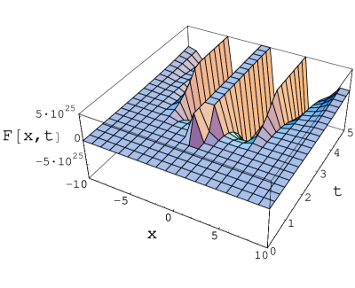
Figure 1: The evolution of the field $F(x,t)$ in the collision of two bubbles. A gluonic wall seems to form in the middle.

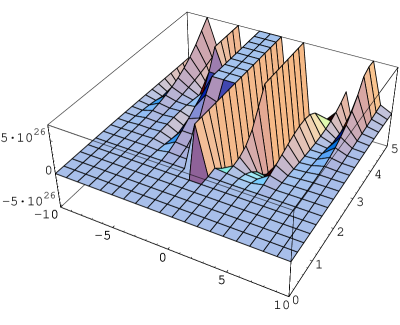
Figure 2: Numerical error estimated by the gauge constraint equation, $C(x,t)=x\partial_{t}F+t\partial_{x}F=0$.

However, we found that this numerical result is not really reliable for several reasons. First of all, notice that the numerical value of $F(x,t)$ drastically changes from the order of $1$ to $\sim 10^{26}$ around $t\simeq 1.1$. It indicates that some singularities occur around at $t\simeq 1.1$ so that the accuracy of the numerical calculations is severely limited beyond this point. Indeed we find that the numerical error estimated by the gauge constraint equation (25) rapidly grows as shown in Fig. 2. While the gauge condition consists of the two terms, the combination of the two terms should not be larger than each individual term in order for the error to be reasonably small. However, Fig. 2 shows unreasonably large error beyond $t\simeq 1.1$. The authors in Ref. Johnson:2003ti have also solved Eq. (III.1) numerically for two fields $W_{0}(x,t)$ and $W_{1}(x,t)$, and reached the same conclusion of the formation of gluonic walls. Even in this case, however, we found severe numerical errors as explained in the appendix.

Secondly, note that the singular behavior colliding at $t\simeq 1.1$ occurs much before the expected collision time scale $t\sim 6$. As we mentioned earlier this may not be unreasonable due to the smooth profile of the initial data, but in order to clarify whether this indicates a violation of causality or not it is necessary to analyze the evolution of the profile in much more detail.

Finally, we point out that the way of solving the set of coupled equations (24) and (25) as above should be corrected. In Ref. Johnson:2003ti $F(x,t)$ is assumed to be a function of $\xi=x^{2}-t^{2}$ only. Consequently, the gauge constraint equation (25) is satisfied automatically. Now one may think that the remaining thing to do is solving the second order partial differential equation (24) for any given initial value of $F$ with vanishing $\partial_{t}F|_{t=0}=0$ as in Eq. (26). Regardless of solving Eq. (24), however, the time evolution of $F(x,t)$ is completely determined by its initial value since $F(x,t)$ is assumed to be a function of $\xi=x^{2}-t^{2}$ only. That is, if $F=F_{0}$ at $(x,t)=(x_{0},0)$, it should be that, for any position $(x,t)$ satisfying $x^{2}-t^{2}=\xi_{0}=x_{0}^{2}$ in the future, $F(x,t)=F(x^{2}-t^{2})=F(\xi_{0})=F_{0}$. In other words, the initial value of $F$ must evolve without any change along the $x^{2}-t^{2}=\xi={\rm constant}$ hyperbola. However, we cannot observe such behavior in Fig. 2.

Although $F(x,t)$ is assumed to be a function of $\xi$ only in Ref. Johnson:2003ti , we show that this assumption is indeed the most general solution of the gauge constraint equation (25). Consider the coordinate transformation such that $\xi=x^{2}-t^{2}$ and $\eta=tx$. Then Eq. (25) becomes

$$\partial_{\eta}F(\xi,\eta)=0,$$ (28)

and so the constraint equation can be solved easily, giving that $F(x,t)$ is a function of $\xi=x^{2}-t^{2}$ only. Consequently, Eq. (24) can be rewritten as

$$\xi F^{\prime\prime}(\xi)+2F^{\prime}(\xi)+3F^{2}(\xi)-2\xi F^{3}(\xi)=0,$$ (29)

where $F^{\prime}(\xi)=dF(\xi)/d\xi$. This is simply a second order ordinary differential equation with respect to $\xi$. In other words, the system of problem which was expressed in the two-dimensional space as in Eq. (24) is actually in the one-dimensional space described by $\xi:-\infty\sim\infty$, due to the presence of the gauge constraint equation (25).

Figure 3: The exact solution Eq. (31) in $\xi$-space.

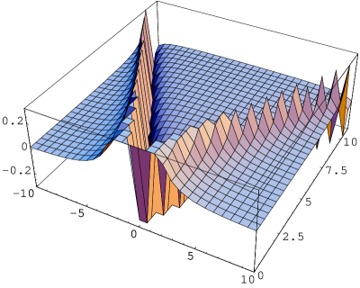
Figure 4: The exact solution Eq. (31) in $(x,t)$-space.

Therefore, giving the initial data for $F(x,t)$ at $t=0$ is equivalent to assigning the value of $F(\xi)$ for $\xi>0$. In the case of Eq. (26), we have

$$F(\xi)=\frac{1}{(\sqrt{\xi}-3)^{2}+\rho^{2}}+\frac{1}{(\sqrt{\xi}+3)^{2}+\rho^{2}}$$ (30)

for $\xi>0$. Now one can easily check that this function above is not a solution of Eq. (29). It implies that one cannot take an arbitrary function of $F(x,0)$ as an initial data set at $t=0$ in Eq. (24). The solution space of Eq. (24) alone is much larger than that of Eq. (29). Only some of them corresponding to a specific class of initial data satisfy Eq. (25) as well at arbitrary time.

(a) $F=-1/2$ and $F^{\prime}=-3/8$ at $\xi=0$. A singular peak occurs at $\xi\simeq 1.6$.

(b) $F=1$ and $F^{\prime}=-3/2$ at $\xi=0$. Singular peaks occur at $\xi\simeq-0.8$ and $-4.0$.

Figure 5: Some numerical solutions for Eq. (29)

We have seen that the correct way of solving the coupled equations (24) and (25) is to solve Eq. (29). What would be the typical behavior of the solutions for Eq. (29)? One can easily see that

$$F(\xi)=\frac{3/2}{\xi}=\frac{3/2}{x^{2}-t^{2}}$$ (31)

is an exact solution of Eq. (29). We see that the singular surface propagates along the light cone, i.e., $\xi=0$ or $x=\pm t$ as shown in Fig. 4. When $F(\xi)$ is not singular at $\xi=0$, we may have the asymptotic solution near $\xi=0$ given by

$$F(\xi)=b-\frac{3b^{2}}{2}\xi+\frac{11b^{3}}{6}\xi^{2}+\cdots.$$ (32)

The numerical solutions for the cases of $b=1,-1/2$ are shown in Fig. 5, respectively.

Figure 6: The time evolution of the numerical solution in Fig. 5 (a) is captured at $t=0,\ 1.0,\ 2.0,\ {\rm and}\ 3.0$, respectively.

Figure 7: The time evolution of the numerical solution in Fig. 5 (b) is captured at $t=0,\ 0.89,\ 1.5,\ 1.97,\ {\rm and}\ 2.2$, respectively.

In $(x,t)$-space, Fig. 5 (a) illustrates a wave initially having two singular peaks at $x\simeq\pm\sqrt{1.6}=\pm 1.26$. As shown in Fig. 6, these two peaks simply propagate away from each other along the hyperbolas $x^{2}-t^{2}\simeq 1.6$, and no formation of a wall can be seen in its future evolution since $|F(x,t)|$ monotonically decreases as $\xi\rightarrow-\infty$. For the case of Fig. 5 (b), the initial wave has a single regular peak located at $x=0$. This peak quickly grows till $t\simeq\sqrt{0.8}=0.894$, splits into two singular peaks which propagate away along the hyperbolas $x^{2}-t^{2}=\xi\simeq-0.8$. At around $t\simeq 2$ a singular peak is formed again, and splits into two singular peaks which propagate away from each other along the hyperbolas $x^{2}-t^{2}=\xi\simeq-4$ as shown in Fig. 7 explicitly.

Therefore, we do not observe the formation of a wall through the collision of two bubbles in this model. Even if a wall is formed ‘spontaneously’, as in Fig. 7, it splits into two parts immediately, propagating away from each other faster than the speed of light. The peak does not last in the region of collision. This property and the violation of the causality should be expected in the region of $\xi<0$ basically because $F(x,t)$ is the function of $x^{2}-t^{2}=\xi$. In the next section, we discuss where the problematic features of this instanton-inspired model come from, and present our new model based on the conventional Lorentzian theory.

III.2 New Lorentzian model

In this section we point out that the instanton-inspired model in which the dynamics of bubble collisions were studied above is actually problematic as a Lorentzian theory. Let us go back to the construction of such model in Eq. (11). Under the Wick rotation such as $x^{4}=\tau\rightarrow\tau=it$ and $x^{i}\rightarrow x^{i}$ for $i=1,2,3$ the relationships between fields in Lorentzian and Euclidean spaces become

$$A^{a}_{t}=i\tilde{A}^{a}_{\tau},\qquad A^{a}_{i}=\tilde{A}^{a}_{i},\qquad\eta^{1}_{t1}=\eta^{2}_{t2}=\eta^{3}_{t3}=\tilde{\eta}^{1}_{\tau 1}=\cdots=-i,\qquad\eta^{1}_{23}=\tilde{\eta}^{1}_{23}=1,$$ (33)

where $\eta^{a}_{\mu\nu}$ is the $\eta$-symbol in Lorentzian space corresponding to the Euclidean t’Hooft symbol $\tilde{\eta}^{a}_{\mu\nu}$ Mueller:1991fa . Thus, the relationships between colored vector fields $A^{a}_{\mu}$ in the original Lorentzian action in Eq. (1) and fields $W_{\mu}$ in the instanton-inspired model in Eq. (11) are indeed

$$A^{a}_{\mu}=\left(\begin{array}[]{cccc}-iW_{1}&-iW_{t}&W_{3}&-W_{2}\\ -iW_{2}&-W_{3}&-iW_{t}&W_{1}\\ -iW_{3}&W_{2}&-W_{1}&-iW_{t}\end{array}\right).$$ (34)

Since the fields $W_{\mu}$ are supposed to be real functions in the instanton-inspired model, it implies that the dynamics for the fields $W_{\mu}$ in this theory is not usual as in ghost-like dynamics in a scalar field system where the scalar field is replaced by an imaginary field, e.g., $-\partial_{\mu}\phi\partial^{\mu}\phi=\partial_{\mu}\psi\partial^{\mu}\psi$ with $\phi=i\psi$. Therefore, although the instanton-inspired model in Eq. (11) was constructed in order to describe bubble collisions in Minkowski space starting from instantons at $t=0$, its dynamics is not the correct Lorentzian one due to the appearance of the imaginary electromagnetic fields. Furthermore, it gives rise to the indefiniteness in the energy density for the fields, e.g., $T_{00}\sim-(\vec{E}^{a})^{2}+(\vec{B}^{a})^{2}$. Notice also that the singular surface of the solution Eq. (20) in the instanton-inspired model expands faster than the speed of light. Thus, it appears to violate the causality.

One may try to redefine some of $W_{\mu}$ fields to absorb the imaginary numbers. However, such prescription turns out to be impossible as can be immediately seen in Eq. (34). Thus, we consider the following model that may describe the Lorentzian bubble dynamics correctly in the vicinity of contacting surface;

$$A^{a}_{\mu}(x,t)=\left(\begin{array}[]{cccc}\psi(x,t)&\varphi(x,t)&0&0\\ 0&0&\varphi(x,t)&\chi(x,t)\\ 0&0&-\chi(x,t)&\varphi(x,t)\end{array}\right).$$ (35)

This form of fields was obtained from Eq. (34) by setting $W_{2}=W_{3}=0$ with plane wave symmetry along $y$ and $z$ directions.

With this ansatz Eq.(5) becomes

$$\partial^{2}\varphi-2g(\chi\varphi^{\prime}-\varphi\chi^{\prime})-2g^{2}\varphi(\varphi^{2}+\chi^{2})=0$$ (36)

$$\partial^{2}\psi-2g(\chi\dot{\varphi}-\varphi\dot{\chi})-2g^{2}\psi(\varphi^{2}+\chi^{2})=0$$ (37)

$$\partial^{2}\chi+2g(\psi\dot{\varphi}-\varphi\varphi^{\prime})-g^{2}\chi(2\varphi^{2}-\psi^{2}+\chi^{2})=0$$ (38)

$$2g(\psi\dot{\chi}-\chi\varphi^{\prime})-g^{2}\varphi(\psi^{2}+\chi^{2})=0,$$ (39)

and the Lorentz gauge condition becomes

$$\dot{\psi}-\varphi^{\prime}=0.$$ (40)

Here $\dot{\varphi}=\partial_{t}\varphi$, $\varphi^{\prime}=\partial_{x}\varphi$, etc. Thus, we have three second-order partial differential equations for three unknown functions $\varphi,\psi$ and $\chi$. Two first-order partial differential equations serve as constraint equations. The energy density in this model is given by

$$T_{00}(x,t) = \frac{1}{2}\left[\left(E^{a}(x,t)\right)^{2}+\left(B^{a}(x,t)\right)^{2}\right]$$ (41)

$$= \frac{1}{2}\Bigg{[}2\left(g\chi\psi+\partial_{t}\varphi\right)^{2}+2\left(-g\varphi\psi+\partial_{t}\chi\right)^{2}+\left(\partial_{t}\varphi-\partial_{x}\psi\right)^{2}+g^{2}\left(3\varphi^{4}+\chi^{4}\right)$$

$$+4g\varphi\chi\partial_{x}\varphi+4g\varphi^{2}\left(g\chi^{2}-\partial_{x}\chi\right)+2\left(\left(\partial_{x}\varphi\right)^{2}+\left(\partial_{x}\chi\right)^{2}\right)\Bigg{]}.$$

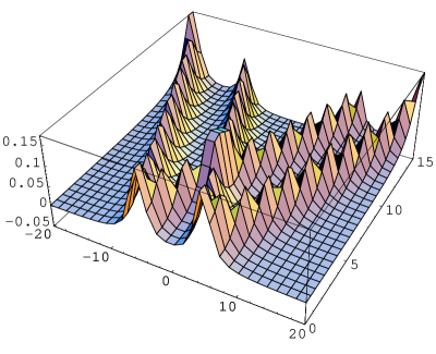
(a) The evolution of the $\chi(x,t)$ field

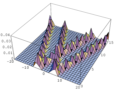
(b) Energy density $T_{00}(x,t)$

Figure 8: The collision of bubble walls in the simplified case of $\varphi=\psi=0$ and $\chi\not=0$

In general, it would be very hard to solve the set of equations (36-40) above. Presumably, we have to solve the constraint equations (39) and (40) first, and then apply it to the dynamical equations (36-38) as was done above for the case of $F$-dynamics in Eqs. (24) and (25). However, we do not know how to solve the constraint equations in general as yet. Let us consider some special cases first.
$(i)$ For the case of $\chi=0$, Eq. (39) gives either $\varphi=0$ or $\psi=0$. If $\varphi=0$, Eqs. (36) and (38) are satisfied, Eq. (40) gives $\dot{\psi}=0$, and Eq. (37) becomes equivalent to a static potential problem in abelian theory, i.e., $\psi^{\prime\prime}(x)=0$. If $\psi=0$, on the other hand, Eq. (40) gives $\varphi^{\prime}=0$, Eqs. (37) and (38) are satisfied, and Eq. (36) becomes

$$\ddot{\varphi}(t)+2g^{2}\varphi^{3}(t)=0.$$ (42)

The exact solution for this homogeneous field $\varphi(t)$ is given by the Jacobi cn function which is periodic in time.
$(ii)$ For the case of $\psi=0$, Eq. (40) gives $\varphi^{\prime}=0$ and one finds either $\chi=0$ or $\varphi=0$ from Eq.(39). If $\chi=0$, we have Eq. (42) above. If $\varphi=0$, on the other hand, Eq. (38) gives

$$\partial^{2}\chi(x,t)-g^{2}\chi^{3}(x,t)=0.$$ (43)

Since the constraint equations are solved already with $\varphi=\psi=0$, the remaining thing is to solve this single second order partial differential equation only. The numerical evolution of two initial peaks for the $\chi(x,t)$ field is shown in Fig. 8. Here the initial data and boundary condition are given by

$$\chi(x,t)|_{t=0}=\frac{1}{4}\left[\frac{1}{(x-5)^{2}+1}+\frac{1}{(x+5)^{2}+1}\right],\quad\partial_{t}\chi|_{t=0}=0,\quad\chi(-20,t)=\chi(20,t)$$ (44)

with $g=1$. Although a rather small peak is likely forming in the middle, two bubble walls pass away in a short time as in the case of linear waves. Thus, our result seems to indicate no formation of a wall through bubble collisions in this simple model.
$(iii)$ For the case of $\varphi=0$, Eq. (39) gives either $\psi=0$ or $\dot{\chi}=0$. If $\psi=0$, we have Eq. (43) above. If $\dot{\chi}=0$, on the other hand, Eqs. (37) and (38) together with Eq. (40) result in

$$\psi^{\prime\prime}(x)-2g^{2}\psi(x)\chi^{2}(x)=0,\qquad\chi^{\prime\prime}(x)-g^{2}\chi(x)(\chi^{2}(x)-\psi^{2}(x))=0.$$ (45)

This case is a static system, which is of no interest for studying dynamical process of bubble collisions. Thus, we find that the non-vanishing field $\chi(x,t)$ with $\varphi=\psi=0$ is the simplest case for dynamical bubble collisions in the new Lorenzian model (35), and it appears no formation of a bubble wall in such simplified case.

Now let us consider bubble collisions in the full model. Since we are unable to solve the constraint equations in this general case as yet, we cannot but solve dynamical equations only with numerical method. When the coupling constant $g$ is non-vanishing, it can be eliminated in Eqs. (36-40) by rescaling fields, i.e., $\varphi\rightarrow\varphi/g$, $\psi\rightarrow\psi/g$, and $\chi\rightarrow\chi/g$. Hence we set $g=1$ in the following analysis. To solve the coupled second order partial differential equations (36-38) numerically we take initial data as

$$\chi_{0}(x)=\chi(x,t)|_{t=0}=\frac{1}{(x-7)^{2}+1}+\frac{1}{(x+7)^{2}+1},\quad\varphi_{0}(x)=\psi_{0}(x)=\chi_{0}(x),$$

$$\dot{\varphi}_{0}(x)=\partial_{t}\varphi|_{t=0}=-1000\frac{\tanh(x/100)}{x^{2}+100}.$$ (46)

The initial data for $\dot{\chi}_{0}(x)$ and $\dot{\psi}_{0}(x)$ are chosen so that the first order equations (39) and (40) are satisfied. At $x=\pm 20$ we give the periodic boundary conditions

$$\varphi(-20,t)=\varphi(20,t),\qquad\psi(-20,t)=\psi(20,t),\qquad\chi(-20,t)=\chi(20,t).$$ (47)

Our numerical results for this set of initial data are shown in Fig. 9. The evolution of the gluon fields $\varphi$, $\psi$ and $\chi$ can be seen in Fig. 9 (a) in the range of time: $t=0\sim 8.51$, and the change of the corresponding energy density is shown in (d). In Fig. 9 (d) a wall seems to appear at around $t\sim 4.5$. Since the constraint equations (39) and (40) are almost fulfilled at least until around $t\sim 4.5$ as can be checked in Fig. 9 (b) and (c), this may indicate a formation of bubble wall indeed.

We also have considered some other sets of initial data. Fig. 10 shows our numerical results for $\varphi_{0}=\psi_{0}=0.3\chi_{0}$, $0.05\chi_{0}$, and $0.01\chi_{0}$ with $\dot{\varphi}_{0}=-100\tanh(x/100)/(x^{2}+100)$. Formation of bubble wall occurs for all three cases as well although the moment of bubble wall formation differs depending on the value of initial data. As in the previous case, the first-order constraint equations are almost fulfilled until around the time from which bubble wall starts to form. Note that, in a longer time, the evolution of two initial peaks for small $\varphi_{0}$ and $\psi_{0}$ is very much different from that for the case of vanishing $\varphi$ and $\psi$ in Eq. (43) even if they are similar in early time. It implies that the presence of all non-vanishing three fields $\varphi$, $\psi$ and $\chi$ in our model is necessary for the formation of bubble wall during collisions.

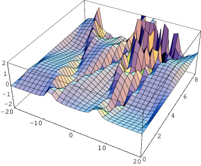
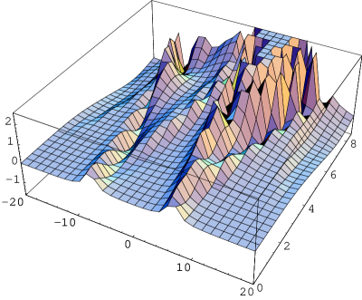
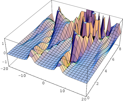
(a) The evolution of the gluon fields $\varphi(x,t)$, $\psi(x,t)$, and $\chi(x,t)$

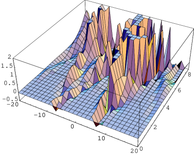
(b) Evaluation of the LHS of the constraint equation (39)

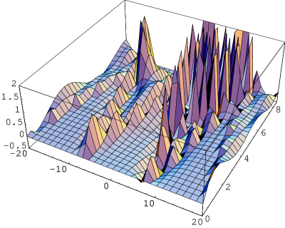
(c) Evaluation of the LHS of the constraint equation (40)

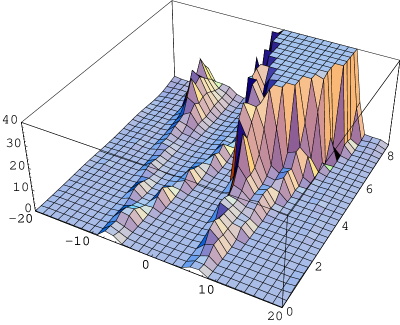
(d) Energy density $T_{00}(x,t)$ in Eq. (41) with $g=1$

Figure 9: The collision of bubble walls in the full model

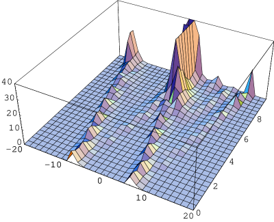
(a) $\varphi_{0}=\psi_{0}=0.3\chi_{0}$

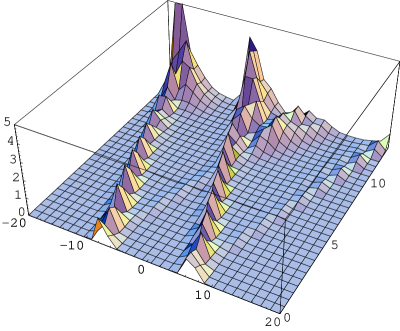
(b) $\varphi_{0}=\psi_{0}=0.05\chi_{0}$

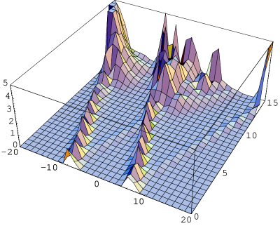
(c) $\varphi_{0}=\psi_{0}=0.01\chi_{0}$

Figure 10: The energy density for various initial values of $\varphi$ and $\psi$. The formation of bubble wall appears at around $t\sim 7.5,\,10.5$, and $11.0$, respectively.

IV Conclusions and Discussions

In this work, we have considered the collision of gluonic bubbles in the context of the instanton-inspired model of QCD phase transition bubbles discussed in Refs. Kisslinger:2002py ; Kisslinger:2002mu ; Johnson:2003ti . In particular, it has been investigated the possibility of bubble wall formation during pure gluonic bubble collisions in plane wave approximation.

Since we are dealing with a system of coupled nonlinear equations of the color dynamics, there exist both dynamical equations and constraint equations in this color dynamics. Correct approach to solve these kinds of system is to solve the constraint equations first and then apply to the dynamical equations. In the case of $F$-dynamics in Eqs. (24) and (25), we can find even an exact solution in this way. Our $F$-dynamics case corresponds to the holonomic constrained system. For other cases, the problems are much harder because the constraints are not easily removed. At present, we cannot but solve these problems with numerical method. However, we checked that our numerical results satisfy the first-order constraint equations, up to some small error, till the appearance of bubble wall formation.

With this correct approach described above we reanalyzed the $F$-dynamics in Eqs. (24) and (25), and found no indication of the bubble wall formation in colliding processes. Moreover, it is pointed out that the instanton-inspired model studied in Refs. Kisslinger:2002py ; Kisslinger:2002mu ; Johnson:2003ti (i.e., Eq. (34) with $W_{2}=W_{3}=0$) should be corrected due to the presence of imaginary gluon fields, since it leads to the violation of causality. Therefore, we reconsidered the process of bubble collisions in a new slightly modified Lorentzian model (35) where we have three independent real gluon fields. For the case of $\chi$-dynamics with $\varphi=\psi=0$ in Eq. (43), we did not find any evidence of the bubble wall formation. For more complicated cases in Eqs. (36)-(40), however, we see some indication of forming the bubble wall. It is likely that the presence of all non-vanishing three gluon fields is necessary to have the formation of bubble wall in collisions.

Nevertheless, we stress that much more careful analyses are necessary to confirm our results. Although the bubble wall formation occurs in the colliding region of two peaks, the location is not exactly the colliding point except for the case of Fig. 10 (a). As can be seen in Fig. 9 (b) and (c), the first-order equations are not satisfied well beyond the time of bubble wall appearance. Consequently, the numerical results beyond this time may not be trustworthy in Figs. 9 and 10. The unexpected appearance of peaks at the left end in late time evolution in Figs. 9 and 10 may be related to this increasing error as time goes by. It will be of great interest to see how the bubble wall formed actually evolves afterwards.

Investigations on solving the constraint equations for the complicated cases are in progress. The idea of applying canonical transformations to the color-dynamic constrained system as in the case of $F$-dynamics may deserve further consideration.

APPENDIX: More Details of Error Estimates

Since the analysis based on Eq. (13) for bubble collisions is severely constrained both in the number of degrees of freedom and the form of the function $F(x,t)$, one may consider an extension to the study with the larger degrees of freedom using $W_{0}$ and $W_{1}$. Note that the set of equations (III.1) and (23) for $W_{0}$ and $W_{1}$ consists of two coupled second-order partial differential equations with one first-order equation in time. As explained in the case of $F$-dynamics in Eqs. (24) and (25), the solution for Eq. (III.1) should satisfy the constraint equation (23) as well. In general, not all solutions for Eq. (III.1) fulfill Eq. (23). Since it is not easy to solve the constraint equation for this case, in contrast to the case of $F$-dynamics, we cannot but solve the dynamical equations (III.1) numerically for certain initial data.

Since the evolution equations in (III.1) are second-order, one can take any initial data set of $W_{0}(x,0)$, $W_{1}(x,0)$, $\partial_{t}W_{0}=\dot{W}_{0}(x,0)$ and $\partial_{t}W_{1}=\dot{W}_{1}(x,0)$ at $t=0$ subject to the first-order equation (23) evaluated at $t=0$ being satisfied (i.e., $\dot{W}_{1}(x,0)=\partial_{x}W_{0}(x,0)$). The case of $F$-dynamics in Eq. (26) corresponds to the special case of $W_{1}(x,0)=\frac{2}{g}xF(x,0)$, $W_{0}(x,0)=\dot{W}_{1}(x,0)=0$, and $\dot{W}_{0}(x,0)=-\frac{2}{g}F(x,0)$. In Ref. Johnson:2003ti the authors consider a somewhat restricted set of initial data such that $W_{0}(x,0)=c$, $W_{1}(x,0)=w(x)$, $\dot{W}_{0}(x,0)=0$, and $\dot{W}_{1}(x,0)=0$.  This initial data set satisfies the gauge condition Eq. (23), and the equations of motion evaluated at $t=0$ are written as

$$\partial_{x}w(x)=g(w^{2}-c^{2})+\frac{1}{2gc}\ddot{W}_{0}(x,0),$$ (48)

$$\partial^{2}_{x}w(x)=2g^{2}w(w^{2}-c^{2})+\ddot{W}_{1}(x,0),$$ (49)

through which the values of $\ddot{W}_{0}(x,t)$ and $\ddot{W}_{1}(x,t)$ at $t=0$ can be determined. However, the authors in Ref. Johnson:2003ti restricted the initial data set further somehow into the case of $\ddot{W}_{0}(x,0)=\ddot{W}_{1}(x,0)=0$. For such case the function $w(x)$ is determined as

$$w(x)=-c\tanh[cg(x-x_{0})].$$ (50)

Here $x_{0}$ is an integration constant.

As mentioned above, however, one can take in general any function $w(x)$ as an initial profile subject to some unknown restriction due to the presence of the unsolved constraint equation. Authors in Ref. Johnson:2003ti used a symmetric ansatz for an initial profile of $w(x)$ given by

$$w(x)=-c\left\{1/2+\tanh\left[cg(x-x_{0})\right]\right\}-c\left\{1/2-\tanh\left[cg(x+x_{0})\right]\right\}$$ (51)

with $c=4$, $g=1$, and $x_{0}=3$. They considered the symmetric boundary condition, $W_{i}(-10,t)=W_{i}(10,t)$, and vanishing initial velocities, $\partial_{t}W_{i}(x,0)=0$, for $i=0,\,1$. In this plane wave model, the energy-momentum tensor density $T_{00}(x,t)$ is given by

$$T_{00}(x,t) = 3(\partial_{t}W_{0})^{2}+(\partial_{x}W_{1})^{2}-2\partial_{t}W_{0}\partial_{x}W_{1}-(\partial_{t}W_{1})^{2}-(\partial_{x}W_{0})^{2}$$ (52)

$$+2g\left[2W_{1}^{2}\partial_{t}W_{0}-W_{0}W_{1}(\partial_{x}W_{0}+\partial_{t}W_{1})\right]+2g^{2}W_{1}^{2}(W_{1}^{2}-W_{0}^{2})+{\cal L}^{\rm glue}$$

in terms of the fields $W_{0}(x,t)$ and $W_{1}(x,t)$. Here ${\cal L}^{\rm glue}$ represents the gluonic Lagrangian density given by

$${\cal L}^{\rm glue} = -\frac{1}{2}\bigg{\{}3(\partial_{t}W_{0})^{2}+3(\partial_{x}W_{1})^{2}-2(\partial_{t}W_{1})^{2}-2(\partial_{x}W_{0})^{2}-2\partial_{t}W_{0}\partial_{x}W_{1}$$ (53)

$$+4g\left[W_{1}^{2}\partial_{t}W_{0}+W_{0}^{2}\partial_{x}W_{1}-W_{0}W_{1}(\partial_{t}W_{1}+\partial_{x}W_{0})\right]+3g^{2}(W_{1}^{2}-W_{0}^{2})^{2}\bigg{\}}.$$

Note that the Lagrangian density in Ref. Johnson:2003ti has the opposite sign of it with the absence of the fifth term above.

(a) $T_{00}(x,0)$

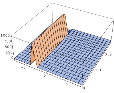
(b) $-T_{00}(x,t)$

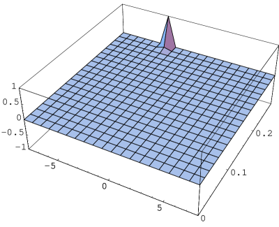
(c) $\partial_{x}W_{0}-\partial_{t}W_{1}$

Figure 11: A numerical solution up to $t=0.28$ in the dynamics of $W_{0}$ and $W_{1}$

As can be seen in Fig. 11 (a), we point out that the energy profile corresponding to the initial data given above is not in the form of two lumps that authors in Ref. Johnson:2003ti expected. The numerical solution evolved up to $t=0.28$ is shown in Fig. 11 (b). One can see in Fig. 11 (c) that the constraint equation $\partial_{x}W_{0}-\partial_{t}W_{1}=0$ is satisfied well up to $t\simeq 0.28$ since $|\partial_{x}W_{0}-\partial_{t}W_{1}|$ is very small in comparison with $|\partial_{x}W_{0}|,\,|\partial_{t}W_{1}|$ whose numerical values turn out to be the order of $\sim 1$. This numerical calculation was able to be performed up to $t=0.28$ by using the NDSolve program in MATHEMATICA. However, if we request plotting the result further beyond $t=0.28$, MATHEMATICA gives it by performing extrapolations which are illustrated in Fig. 12.

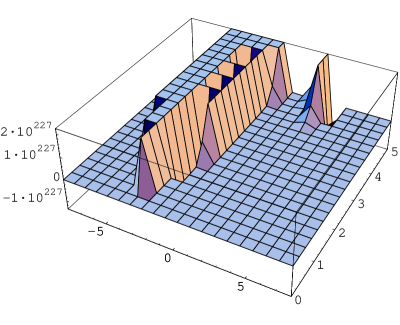
(a) $-T_{00}(x,t)$

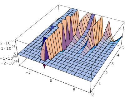
(b) $\partial_{x}W_{0}-\partial_{t}W_{1}$

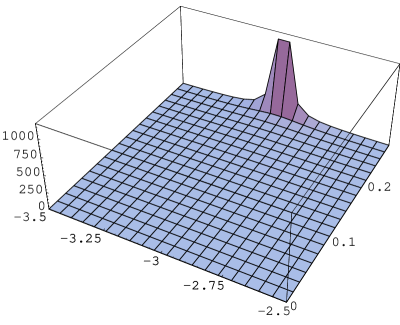
(c) $W_{0}(x,t)$

Figure 12: The extrapolated solution up to $t=5$ in the dynamics of $W_{0}$ and $W_{1}$

One can see that this extrapolated energy density changes drastically around $t=0.28$ from the order of $10^{3}$ to the order of $10^{227}$, indicating a singular behavior of solution. One might think that the peak shown in Fig. 12 (a) is an indication of the bubble wall formation as discussed in Ref. Johnson:2003ti . However, it is hard to think that an initially single peak develops a bubble wall. The consideration of other type of initial data giving an energy profile of two peaks would be necessary. Fig. 12 (b) also shows that the constraint equation is not satisfied well for this extrapolated solution since $|\partial_{x}W_{0}|,\,|\partial_{t}W_{1}|$ becomes the order of $10^{58}$ which is almost same as the order of $|\partial_{x}W_{0}-\partial_{t}W_{1}|$. For these reasons, therefore, we think that more careful analysis is needed on the bubble collision in the dynamics of $W_{0}$ and $W_{1}$.

References

- (1) See, e.g., website “http://www.bnl.gov/RHIC”.
- (2) See, e.g., website “http://www.esf.org/esf_article.php?activity=1&article=7&domain=1”.
- (3) W. Thirring, Ann. Phys. 3, 91 (1958).
- (4) J. K. Perring and T. R. H. Skyrme, Nucl. Phys. 31, 550 (1962).
- (5) J. von Neumann, Mathematical Foundations of Quantum Mechanics, Princeton, NJ, Princeton University Press, 1955.
- (6) S. Coleman, Phys. Rev. D 15, 2929 (1977); 16,1248(E); C. Callan, S. Coleman, Phys. Rev. D 16, 1762 (1977); Phys. Rev. 177, 2247 (1969); S. Coleman, Aspects of Symmetry, Cambridge University Press, 1985.
- (7) S. W. Hawking, I. G. Moss and J. M. Stewart, Phys. Rev. D 26, 2681 (1977).
- (8) T. W. B. Kibble and A. Vilenkin, Phys. Rev. D 52, 679 (1995); J. Ignatius, K. Kajantie, H. Kurki-Suonio and M. Laine, Phys. Rev. D 50, 3738 (1994); Phys. Rev. D 49, 3854 (1994); J. C. Miller and L. Rezzolla, Phys. Rev. D 51, 4017 (1995); M. B. Christiansen and J. Madsen, Phys. Rev. D 53, 5446 (1996); E. Farhi, V. V. Khoze and R. Singleton, Jr., Phys. Rev. D 47, 5551 (1993); K. Geiger, Phys. Rev. D 51, 3669 (1995); G. Neergaard and J. Madsen, Phys. Rev. D 53, 5446 (1996); Phys. Rev. D 62, 034005 (2000).
- (9) M. M. Forbes and A. R. Zhitnitsky, JHEP 0110, 013 (2001); Phys. Rev. Lett. 85, 5268 (2000); hep-ph/0102158 (2001).
- (10) J. Ahonen and K. Enqvist, Phys. Rev. D 57, 664 (1998).
- (11) E. J. Copeland, P. M. Saffin and O. Tornkvist, Phys. Rev. D 61, 105005 (2000).
- (12) L. S. Kisslinger, “Instanton model of QCD phase transition bubble walls,” [arXiv:hep-ph/0202159].
- (13) L. S. Kisslinger, Phys. Rev. D 68, 043516 (2003) [arXiv:hep-ph/0212206].
- (14) M. B. Johnson, H. M. Choi and L. S. Kisslinger, Nucl. Phys. A 729, 729 (2003) [arXiv:hep-ph/0301222].
- (15) S. W. Hawking, Nature 248, 30 (1974); Commun. Math. Phys. 43, 199 (1975) [Erratum-ibid. 46, 206 (1976)].
- (16) M. Visser, Phys. Rev. Lett. 80, 3436 (1998); W. G. Unruh, Phys. Rev. Lett. 46, 1351 (1981); Phys. Rev. D 51, 2827 (1994).
- (17) “Cosmic Problems for Condensed Matter Experiment,” arXiv:cond-mat/0404480.
- (18) Y. Mishchenko and C.-R. Ji, Phys. Rev. D 68, 063503 (2003).
- (19) M. Persic, P. Salucci and F. Stel, Mon. Not. R. Astron. Soc. 281, 27 (1996).
- (20) D. H. Oaknin and A. Zhitnitsky, Phys. Rev. D 94, 101301 (2005); Phys. Rev. D 71, 023519 (2005).
- (21) G. ’t Hooft, Phys. Rev. D 14, 3432 (1976).
- (22) A. A. Belavin, A. M. Polyakov, A. S. Schvarts and Yu. S. Tyupkin, Phys. Lett. B 59, 85 (1975); T. Schäfer and E. V. Shuryak, Phys. Rev. D 53, 6522 (1996); Rev. Mod. Phys. 70, 323 (1998); M-C. Chu and S. Schramm, Phys. Rev. D 51, 4580 (1995); D 62, 094508 (2000); E. Shuryak and I. Zahed, Phys. Rev. D 62, 085014 (2000); M. A. Nowak, E. V. Shuryak and I. Zahed, Phys. Rev. D 64, 034008 (2001).
- (23) E. V. Shuryak, Phys. Rept. 61, 71 (1980).
- (24) A. H. Mueller, Nucl. Phys. B 364, 109 (1991).