Nonequilibrium field theory from the 2PI effective action

Abstract:

Nonperturbative approximation schemes are inevitable even in weakly coupled theories if the nonequilibrium behavior of quantum fields is investigated. The two-particle irreducible (2PI) effective action formalism provides an efficient framework for obtaining resummation schemes both in and out of equilibrium. We briefly review the these techniques and discuss recent findings for nonequilibrium field theories.

1 Introduction

The new observations of the heavy ion collider facilities represent a great challenge to particle field theory. The achieved volume and life time of the produced hot and dense matter may now enable thermalization. On the other hand, due to the developments on the theory side, calculations of nonequilibrium processes become increasingly feasible.

It has been recently observed that the phenomenological description of particle flow based on ideal hydrodynamics is extremely successful at RHIC energies [1]. The used models assume local equilibrium already before 1 fm/c. The competence of ideal hydrodynamics indicates a very early thermalization of the produced plasma [2]. A further signal of an at least partial equilibration is that the global abundances from collision experiments obey simple statistical models assuming chemical equilibrium [3].

The observed early onset of equilibrium calls for a novel theoretical paradigm. The perturbative thermalization time estimates are far beyond the experimental expectations. As a first step one has to understand, what level of equilibration is required to interpret the experimental data. The success of ideal hydrodynamical description might be explained by the early onset of an isotropic equation of state [4] that may be present even in a far-from-equilibrium quantum field [5]. Then one seeks for explosive processes that drive the system towards isotropy and equilibrium. A promising candidate is the development of plasma instabilities that may dramatically accelerate the evolution of anisotropic fields [6, 7].

Nonequilibrium methods are also asked for in early Universe scenarios. Much of the efforts have been put into the quantitative understanding of the theory of reheating, which explains the rapid re-population of the dilute Universe after inflation [8]. The final temperature is an important input to models of baryogenesis [9].

The intriguing questions of non-thermal field evolution cannot be answered by a simple perturbative analysis. Even in a weakly coupled theory high orders become relevant with the evolution of the time. The elapsed time appears next to the coupling constant, making the effective coupling arbitrarily big at late times. This phenomenon, called secularity, invalidates approximations that truncate higher order diagrams in the equation of motion of the Green’s function [10]. A way to evade this trap is to use self-consistent schemes [11].

There has been important progress in our understanding of nonequilibrium quantum fields using suitable resummation techniques based on two-particles-irreducible (2PI) generating functionals [12]. It has been shown by Cox and Berges [13] that the Kadanoff-Baym equations are suitable for direct numerical treatment. They used the 2PI effective action formalism [14] to calculate the self energies in as systematic way. They found that the studied scalar field reaches thermal equilibrium even in 1+1 dimensions, where binary collision are forbidden by kinematics on the level of the Boltzmann equation.

The 2PI effective action techniques (or $\Phi$ derivable approximations) are known to provide time reversal symmetric, energy conserving equations for the field propagator [11]. The equations involve the resummation of those diagrams that carry the time in the effective coupling, this cures the secularity of the perturbative treatment.

The 2PI equations of motion have been solved for various models since the pioneering work by Cox and Berges [13]: ranging from the simplest $\Phi^{4}$ scalar theory [32, 29, 30] through the scalar O($N$) theory with next–to–leading order large $N$ resummation [15, 16, 17, 18, 19, 20] to the chiral meson model [21], often considered as a prototype of QCD.

The 2PI formalism was used to show for the first time from first principles the formation of the Bose-Einstein and Fermi-Dirac statistics in a system of coupled fermions and scalars [21]. The used equations do not involve any of the statistical factors or constraints for the occupation numbers, not even the concept of particles. The resulting distributions are purely an outcome of the coupled field dynamics (See Fig. 1).

     

Figure 1: Evolution of the particle distribution function in the chiral quark model [21]. To the left, the fermionic particle spectrum is shown for various times. The spectra have been transformed so that a linear corresponds to the Fermi-Dirac statistics. To the right, the final distribution is displayed without the transformation. The coupled system of fermions and scalars dynamically realizes the Fermi-Dirac and Bose-Einstein statistics.

In the next sections we first review the 2PI effective action formalism on the example of a scalar theory. Then we discuss the various resummations necessary to calculate the self-consistent $n$-point functions to the desired accuracy. The 2PI results have been checked both in equilibrium and out of equilibrium, we briefly mention the main results of these tests. We also highlight some of the numerical results on the basic time scales of nonequilibrium evolution.

2 The formalism

The objective is to give an equation for the propagator and also for the higher $n$-point functions of an evolving field. The 2PI formalism does not use the concept of quasi-particles, it establishes the relationship between various $n$-point functions in a systematic truncation scheme. To keep this review simple, we restrict our discussion to the scalar propagator, which already gives account for the evolution of particle distribution. The equations are worked out for higher $n$-point functions in Ref. [22]. The 2PI formalism for multiple scalar fields is discussed in detail in Refs. [16, 23], for fermionic fields it has been elaborated in Refs. [21, 24]. For renormalizable theories the 2PI equations of motion are also renormalizable, the correct way to define a finite theory has been discussed by many authors [25, 26, 22, 23, 24]. The interested reader is referred to the in-depth review in Ref. [12].

The proper two-point function, that we are looking for, is defined in terms of the one-particle irreducible (1PI) effective action:

$$\mathcal{G}^{-1}(x,y)=-i\frac{\delta^{2}\Gamma[\phi]}{\delta\phi(x)\delta\phi(y)}$$ (1)

In the case of more than one field components $\mathcal{G}$ is a matrix in the field indices as well as in the space-time coordinates.

The $\Gamma[\phi]$ effective action is now a functional of the space and time dependent background field. A straightforward approximation would be a coupling expansion in $\Gamma[\phi]$. A danger in this approach is, that a Taylor expansion in $\phi$ simply cancels the higher proper $n$-point functions. Negative results warn us that it is required to include high powers of $\phi$ in the effective action. This can be achieved by imposing the truncation to the Legendre transform of $\Gamma[\phi]$. This way we selectively resum 1PI diagrams to infinite order.

The two-particle irreducible (2PI) effective action is defined as a Legendre transform of the effective action with respect to the source $K(x,y)$ of the two-point composite field operator ($\phi(x)\phi(y)$):

$$\Gamma_{\rm 2PI}\left[\phi,\mathcal{G}[\phi,K]\right]=\Gamma[\phi]-\frac{1}{2}\int\limits_{\mathcal{C}}\mbox{d}{}^{4}x\int\limits_{\mathcal{C}}\mbox{d}{}^{4}y\left(\mathcal{G}[\phi,K](x,y)K(x,y)+\phi(x)K(x,y)\phi(y)\right)\,.$$ (2)

The subscript $\mathcal{C}$ refers to the closed time path (CTP) contour for the time integral.

The second argument of the 2PI effective action $\Gamma_{\rm 2PI}[\phi,G]$ is a generic two-point function $G(x,y)$. For any given $\phi$ background and vanishing sources

$$\frac{\delta\Gamma_{\rm 2PI}\left[\phi,G\right]}{\delta G\left(x,y\right)}=0\;,$$ (3)

with $G=\mathcal{G}[\phi]$. From $\Gamma_{\rm 2PI}$ it is straightforward to go back to the 1PI effective action using the identity $\Gamma[\phi]=\Gamma_{\rm 2PI}[\phi,\mathcal{G}[\phi]]$.

Unfortunately, the exact $\Gamma_{\rm 2PI}$ functional is not known. Following Cornwall, Jackiw and Tombulis [14] one can decompose the 2PI effective action into tree-level (1st term), one-loop level (2nd and 3rd term) and higher order (4th term) contributions.

$$\Gamma_{\rm 2PI}\left[\phi,G\right] = S\left[\phi\right]+\frac{i}{2}\mbox{tr}_{\mathcal{C}}\left[\log\left[G^{-1}\right]\right]+\frac{i}{2}\mbox{tr}_{\mathcal{C}}\left[G_{0}^{-1}[\phi]G\right]$$

$$+\Gamma_{2}\left[\phi,G\right]+const\;.$$

Here $G_{0}[\phi]$ denotes the free propagator on the background, and $S$ is the classical action. The decomposition (2) defines a term $\Gamma_{2}[\phi,G]$ that can be entirely represented by two-particle irreducible diagrams, i.e. these diagrams do not fall apart if any two of its lines are cut.

We will use a slightly modified decomposition, where the background dependence of the free propagator is put into the interaction part $\Gamma_{\rm int}[\phi,G]$:

$$\Gamma_{\rm 2PI}\left[\phi,G\right] = S\left[\phi\right]+\frac{i}{2}\mbox{tr}_{\mathcal{C}}\left[\log\left[G^{-1}\right]\right]+\frac{i}{2}\mbox{tr}_{\mathcal{C}}\left[G_{0}^{-1}[\phi\equiv 0]G\right]$$

$$+\Gamma_{\rm int}\left[\phi,G\right]+const\;.$$

In the 2PI formalism the truncation is realized by the formal expansion of $\Gamma_{\rm int}[\phi,G]$ in the coupling constant or in an other small parameter, such as the inverse number of field components. There are Feynman rules to construct $\Gamma_{int}$ from the selected diagrams. The most important ingredient of these rules is to write a $G(x,y)$ function for each propagator. For the vertices, however, the bare couplings appear (with counterterms, eventually).

For the most trivial case of scalar $\lambda\Phi^{4}/24$ theory one simply keeps:

$$\Gamma_{\rm int}[G]=-\frac{\lambda}{4}\int\limits_{\mathcal{C}}dx\,\phi(x)G(x,x)\phi(x)-\frac{\lambda}{8}\int\limits_{\mathcal{C}}dx\,G^{2}(x,x)$$

$$+i\frac{\lambda^{2}}{12}\int\limits_{\mathcal{C}}\int\limits_{\mathcal{C}}dxdy\,\phi(x)G^{3}(x,y)\phi(y)+i\frac{\lambda^{2}}{48}\int\limits_{\mathcal{C}}\int\limits_{\mathcal{C}}dxdy\,G^{4}(x,y)\,.$$ (6)

The first two terms correspond to the (collisionless) Hartree approximation [28], the next two terms give account for the “particle collisions” at lowest order. An expansion to higher orders in $\lambda$ is found in Ref. [29].

When using a truncated $\Gamma_{\rm 2PI}$ we have to rethink the exact identities derived so far. We define the resummed two-point function $\bar{G}[\phi](x,y)$ as the solution of Eq. (3) with the truncated $\Gamma_{\rm 2PI}$. Using this as an argument of $\Gamma_{\rm 2PI}$ one uses

$$\Gamma[\phi]=\Gamma_{\rm 2PI}\left[\phi,\bar{G}[\phi]\right]$$ (7)

as a definition for the truncated 1PI effective action [31]. As already noted, this relation turns to an identity in the case without truncation. This truncated $\Gamma[\phi]$ is used then to define $\mathcal{G}$ according to Eq. (1). This $\mathcal{G}(x,y)$ propagator is in general, not identical to $\bar{G}[\phi](x,y)$

As a first step we have to solve Eq. (3), which can be put to the form of a Schwinger-Dyson equation using Eq. (2):

$$\overline{G}^{-1}\left(x,y\right)=G_{0}^{-1}[\phi\equiv 0]\left(x,y\right)-\Sigma\left[\overline{G}[\phi]\right]\left(x,y\right)$$ (8)

with

$$\Sigma[\overline{G}]\left(x,y\right) = 2i\frac{\delta\Gamma_{\rm int}\left[\overline{G}\right]}{\delta\overline{G}\left(x,y\right)}\,.$$ (9)

Here the self energy ($\Sigma$) is built of one-particle irreducible diagrams constructed form resummed lines ($\bar{G}[\phi]$) and bare vertices. (Coming from the first term in Eq. (6) it may actually contain a diagram $\sim\delta_{\mathcal{C}}(x,y)\phi(x)\phi(y)$, which is not 1PI. Using the original decomposition (2) this term would appear in $G_{0}^{-1}[\phi]$.)

In the second step we evaluate the 2PI effective action at $\bar{G}[\phi]$ and calculate $\mathcal{G}$ as follows:

$${\cal G}^{-1}[\phi](x,y)=-i\frac{\delta^{2}\Gamma[\phi]}{\delta\phi(x)\delta\phi(y)}=-i\frac{\delta^{2}\Gamma_{\rm 2PI}[\phi,\overline{G}[\phi]]}{\delta\phi(x)\delta\phi(y)}\,.$$ (10)

Analogously, any higher $n$-point functions are available if $\overline{G}[\phi]$ is known for any $\phi$ background.

In the symmetric phase ($\phi\equiv 0$) Eq. (10) takes a simpler form if the model has the $Z_{2}$ ($\phi\leftrightarrow-\phi$) symmetry:

$${\cal G}^{-1}[\phi\equiv 0](x,y)=G_{0}^{-1}[\phi\equiv 0](x,y)-i\left.\frac{\delta^{2}\Gamma_{\rm int}[\phi,\overline{G}[\phi\equiv 0]]}{\delta\phi(x)\delta\phi(y)}\right|_{\phi\equiv 0}\,.$$ (11)

We emphasize at this point, that in the broken phase additional terms appear [22]. Without these additional terms the propagator $\mathcal{G}$ would violate Goldstone theorem [31, 16].

There are some “friendly” truncations (including Eq. (6)) for which $\Gamma_{\rm int}$ has the symmetry:

$$\left.\frac{\delta^{2}\Gamma_{\rm int}[\phi,G]}{\delta\phi(x)\delta\phi(y)}\right|_{\phi\equiv 0}=\left.2\frac{\delta^{2}\Gamma_{\rm int}[\phi,G]}{\delta G(x,y)}\right|_{\phi\equiv 0}\,.$$ (12)

This further simplifies Eq. (11) to

$${\cal G}[\phi\equiv 0](x,y)=\overline{G}[\phi\equiv 0](x,y)\,.$$ (13)

For a $Z_{2}$ symmetric exact theory Eq. (12) is always granted, as expected, $\mathcal{G}$ and $\overline{G}$ are then equivalent.

All the models numerically investigated so far (the three-loop $\Phi^{4}$ theory, the O($N$) model truncated at next-to-leading order in $1/N$ and the two-loop chiral quark model) have this nice feature. This explains why numerical works directly use the solution of the Schwinger-Dyson equation (8).

3 Evolution equations

Eq. (8) uses complex and nonanalytic functions on CTP contour, thus, it is not suitable for a numerical treatment. Therefore we introduce the statistical propagator $F(x,y)$ and the spectral function $\rho(x,y)$ and the corresponding functions for the self energy, too [32]:

$$\overline{G}(x,y) = F(x,y)-\frac{i}{2}\rho(x,y){\rm sgn}_{\mathcal{C}}(x_{0},y_{0})\,,$$ (14)

$$\Sigma[\overline{G}](x,y) = -i\Sigma_{0}(x)\delta_{\mathcal{C}}(x,y)+\Sigma^{F}(x,y)-\frac{i}{2}\Sigma^{\rho}(x,y){\rm sgn}_{\mathcal{C}}(x_{0},y_{0})\,.$$ (15)

The real ($F$) and imaginary ($\rho$) part capture different physical information: $\rho$ gives what states are available and how stable they are, while $F$ tells how they are occupied. In equilibrium, the $F$ and $\rho$ functions are connected by the KMS condition, but they are a priori independent out of equilibrium. These functions do not depend on contour variables, all discontinuities are encapsulated in the contour delta $\delta_{\mathcal{C}}$ and sign function ${\rm sgn}_{\mathcal{C}}$. One can transform Eq. (8) into integral equations, where the integral is defined on the closed-time-path contour [33]. Using the $F$ and $\rho$ functions in these integral equations the discontinuities appear as boundaries of the time integral. For a scalar field theory, the equations of motion in terms of the $F$ and $\rho$ functions read:

$$\left(\partial_{x}^{2}+m^{2}+\Sigma_{0}(x)\right)F(x,y) = \int\limits^{y_{0}}_{t_{0}}dz\Sigma^{F}(x,z)\rho(z,y)-\int\limits^{x_{0}}_{t_{0}}dz\Sigma^{\rho}(x,z)F(z,y)\,,$$ (16)

$$\left(\partial_{x}^{2}+m^{2}+\Sigma_{0}(x)\right)\rho(x,y) = \int\limits^{y_{0}}_{x_{0}}dz\Sigma^{\rho}(x,z)\rho(z,y)\,.$$ (17)

These equations are exact, the approximation is encoded into the used self energy, given by Eq. (9). Working out the self energy for the model of choice we can close Eqs. (16-17). For the one-component scalar $\lambda\Phi^{4}/24$ theory at three-loop level two diagrams contribute (at $\phi\equiv 0$) [32]

$$\Sigma^{F}(x,y) = -\frac{\lambda^{2}}{6}F(x,y)\left(F^{2}(x,y)-\frac{3}{4}\rho^{2}(x,y)\right)\,,$$ (18)

$$\Sigma^{F}(x,y) = -\frac{\lambda^{2}}{2}\rho(x,y)\left(F^{2}(x,y)-\frac{1}{12}\rho^{2}(x,y)\right)\,.$$ (19)

$$\Sigma_{0}(x) = \frac{\lambda}{2}F(x,x)\,.$$ (20)

The solution of the resulting closed set of equations is not accessible without numerical methods. If the initial ensemble is spatially homogeneous, the two-point functions depend on five variables ($x_{0},y_{0},\vec{x}-\vec{y}$) only.

The actual form of the equations of motion (16-17) depend on the type of the initial conditions. The most simple choice is to assume a known Gaussian density operator at initial time $t_{0}$, the presented form of Eqs. (16-17) reflect this choice. In this case the integrals start form $t_{0}$, and the numerical integration of Eqs. (16-17) is conceptually straightforward (but may be technically involved).

The initial conditions for the second order differential equations can be given by setting $F(x_{0}=t_{0},\vec{x};y_{0}=t_{0},\vec{y})$ and its first order time-derivatives. The $\rho(x_{0}=t_{0},\vec{x};y_{0}=t_{0},\vec{y})$ function is zero identically, its derivative is constrained by Heisenberg‘s commutation relation: $\partial_{x_{0}}\rho(x_{0}=t_{0},\vec{x};y_{0}=t_{0},\vec{y})=\delta(\vec{x}-\vec{y})$.

An initial particle distribution $n_{0}(\vec{p})$ can be easily prescribed using Gaussian initial conditions:

$$F(x^{0},y^{0};\vec{p})|_{x^{0}=y^{0}=t_{0}} = \frac{n_{0}(\vec{p})+1/2}{\omega_{p}}\,,$$ (21)

$$\partial_{x^{0}}\partial_{y^{0}}F(x^{0},y^{0};\vec{p})|_{x^{0}=y^{0}=t_{0}} = [n_{0}(\vec{p})+1/2]\omega_{p}\,,$$ (22)

$$\partial_{x^{0}}F(x^{0},0;\vec{p})|_{x^{0}=t_{0}}=0\,,$$ (23)

with $\omega_{p}\equiv\sqrt{{\vec{p}}^{2}+M_{0}^{2}}$ and $M^{2}_{0}$ is the initial time physical mass. Here the propagators are Fourier transformed in space with respect to the relative coordinate $\vec{x}-\vec{y}$.

4 The resummation scheme

Let us now review the resummations automatized by the 2PI formalism on the simple example of a scalar $\Phi^{4}$ theory. The considered approximation we define by giving the 2PI effective action explicitely in Eq. (6). The corresponding self energy equation (9) can be graphically expressed as seen in Fig. 2. The first two diagrams contribute at leading order to the self energy. The next two terms account for the next-to-leading order effects.

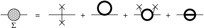
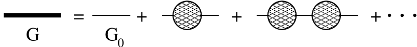
Figure 2: Graphical representation of the 2PI equations of motion. The upper equation shows the self energy in the simple truncation of the scalar $\Phi^{4}$ theory at three loop order. The thick lines stand for the self-consistent propagator ($G$), which is a subject of Dyson resummation (lower equation) using the free propagator (thin lines) and this self energy.

By unrolling these equations and drawing the diagrams contributing to $G$ in terms of the free (or initial time) propagator one reveals the elementary physical processes caught by this scheme. As shown in Fig. 3 a typical diagram is a ladder with finite number of rungs. Thinking of quasi-particles, each of these rungs represents an elementary scattering in the time dependent bath of other particles. One may associate a time scale $\tau$ to these elementary processes. In a period of $n\tau$, $n$ elementary collisions occur per particle on average. Beyond this period of time diagrams with more rungs start becoming relevant, hence higher perturbative orders are necessary. This phenomenon, called secularity, forbids the perturbative treatment of nonequilibrium fields, and calls for the resummation of this chain of ladders. This chain of ladders is what 2PI actually resums.

Figure 3: Nonequilibrium interpretation of the ladder resummation. For any perturbative order there is a time when its contribution starts being relevant. A given order may account for some finite number of elementary collisions. After that number of elementary processes new orders will become of the same order. The 2PI ladder resummation considers all orders and solves the problem of secularity.

If one now tries to calculate a four-point function out of $\Sigma[\bar{G}]$ by cutting a line, one realizes soon that only one of the three possible channels are resummed, the Bose symmetry is broken. This is the reason we did not define the propagator as $\bar{G}$, the solution of the 2PI equations of motion, but used the 1PI effective action instead to introduce the proper two-point function ${\cal G}$ in Eq. (1). The difference between $\bar{G}$ and ${\cal G}$ are diagrammatically exemplified in Fig. 4. In many cases (see Eq. (12)) they agree at $\phi\equiv 0$, therefore we show a selection of $\phi$-dependent diagrams only. The channels missing from $\bar{G}$ can be included by solving a further (Bethe–Salpeter) equation [25, 26, 22]. This equation follows from the definition of ${\cal G}$ without additional theoretical input. In Fig. 5 we give its diagrammatic form, showing the NLO contribution only. One can show for the truncations obeying Eq. (12), that the Bethe–Salpeter equation is the equation of motion for ${\delta^{2}\bar{G}(\phi;x,y)}/{\delta\phi^{2}}$ at vanishing background, which is required to carry out the derivatives in Eq. (1). The four-point box contributes symmetrically in each channel to Eq. (1), this restores the Bose symmetry [31, 22].

Figure 4: Graphs contributing to the $\phi$-dependent part of the 2PI-resummed propagator at next-to-leading order. The 2PI equation of motion resums a ladder in one channel (left hand side). To the proper two-point function ${\cal G}$, however, additional diagrams contribute (right hand side), that play an important role in the broken phase: they make sure that the Goldstone theorem is fulfilled. The missing diagrams can be calculated by solving the Bethe-Salpeter equation.

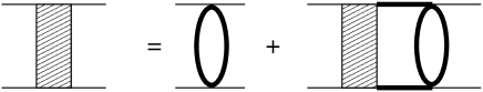
Figure 5: Graphical representation of the Bethe–Salpeter equation. The thick lines stand for the solution of the propagator equation at vanishing background.

The topology of the resummed diagrams become more complicated for the O($N$) symmetric scalar theory in the large $N$ expansion. As detailed in Refs. [15, 16], an additional resummation is required on the level of the 2PI effective action. Then $\Gamma_{\rm int}[\phi,G]$ is already an infinite series of diagrams Fig. 6 (left). By introducing a self-consistent vertex function (see Fig. 6 (right-top)) one may reduce the 2PI effective action to a sum of finite number of 2PI diagrams Fig. 6 (right-bottom). The concept of self-consistent vertex functions can be generalized and made systematic in the context of the $n$-particle irreducible effective actions [39].

This large-$N$ resummation is always necessary if the occupation numbers are large (proportional to the inverse coupling). Any additional loop in Fig. 6 (left) carries additional powers of occupation numbers that compensate the coupling. This typically happens in preheating dynamics of the early universe [18].

           

Figure 6: Large-$N$ resummation in the O($N$) scalar theory. The 2PI effective action to next-to-leading order in $1/N$ consists of an infinite series of diagrams (left panel). These can be resummed by introducing a self-consistent coupling (big dot on the right panel) [16].

2PI can be also used to derive Boltzmann equations. From the 2PI effective action in Eq. (6) one arrives to a kinetic theory that accounts for the $2\to 2$ scattering of quasi-particles [35]. The connection of the 2PI equations with kinetic theories justifies the interpretation of the ladder resummation above, and also makes clear what additional assumptions are made in such theories. Since 2PI does not make these assumptions, it can be used to establish the range of validity of the following steps:

1. The lower bound of the time integral in Eqs. (16-17) is extended to $-\infty$. The equations are often formulated in Wigner transformed form. In order to make use of some mathematical identities to rewrite the equations in a handy form one usually extends the finite integrals in the relative ($x-y$) coordinate to the range $-\infty\dots\infty$. If one does this, the equations do not refer to an initial value problem any more. This introduces an approximation, that is justified from that time $t$ on, when $F(t,t_{0})$ and $\partial_{t}\rho(t,t_{0})$ become small compared to the equal time correlators. This usually occurs around damping time ($t_{\rm damp}$), given by the imaginary part of the self energy [36].

2. Transport equations typically use gradient expansion to make the equations of motion local in time. It is controlled by the smoothness of the evolution, and becomes exact near equilibrium. As expected, in weakly coupled theories subsequent orders of this expansion converge well. The intermediate time description of evolution can be substantially improved by going beyond the usually considered lowest order [36].

3. The transport equation for $\rho$ can be replaced by an assumed relationship between the $F$ and $\rho$ propagators. This nonequilibrium KMS condition parametrized by the particle distribution can be used as an ansatz in the $F$ equation. It has been shown using 2PI equations that this relationship is dynamically established in damping time scale, well before the equilibration of the parametrizing distribution [37].

4. In the final step one replaces the spectral function ($\rho$) by a delta function, and introduces the quasi-particles. A detailed comparison of Boltzmann equation restricted to binary collisions with the 2PI dynamics based on Eq. (6) can be found in Ref. [38].

In summary, these steps are well justified in sufficiently weakly coupled theories, only after the damping time scale. This sets a clear limitation to transport and kinetic theories when they are applied to initial value problems [36].

5 Testing 2PI

5.1 Convergence in equilibrium

Since nonequilibrium description of fields requires non-perturbative treatment we were forced to use a resummation formalism. The same techniques can be applied in thermal equilibrium, too, where efficient formulations in Euclidean space-time become available. In contrast to the far-from-equilibrium case, there are various powerful approximation schemes known in thermal field theory. A prominent approach in equilibrium high-temperature field theory is the so-called “hard-thermal-loop” resummation [41]. However, explicit calculations of thermodynamic quantities such as pressure or entropy typically reveal a poor convergence except for extremely small couplings. An important example for this behavior concerns high-temperature gauge theories. Recent strong efforts to improve the convergence aim at connecting to available lattice QCD results, for which high temperatures are difficult to achieve. In order to find improved approximation schemes it is important to note that the problem is not specific to gauge field theories. Indeed it has been documented in the literature in great detail that problems of convergence of perturbative approaches at high temperature can already be studied in simple scalar theories. For recent reviews in this context see Ref. [42].

A promising candidate for an improved convergence behavior is the loop or coupling expansion of the 2PI effective action. So far, thermodynamic quantities such as pressure or entropy have been mainly calculated to two-loop order. However, aspects of convergence can be sensefully discussed only beyond two-loop order since the one-loop high-temperature result corresponds to the free gas approximation. Efforts to calculate pressure to nontrivial order include so-called approximately self-consistent approximations [43], as well as estimates based on further perturbative expansions in the coupling and a variational mass parameter [44]. These studies indicate already improved convergence properties. However, perturbatively motivated estimates as in Ref. [44] suffer from the presence of nonrenormalizable, ultraviolet divergent contributions and the apparent breakdown of the approach beyond some value for the coupling. If one does not want to rely on these further assumptions, going beyond two-loop order requires the use of efficient numerical techniques. Such rigorous studies are important to get a decisive answer about the properties of 2PI expansions. As it turns out these problems appear as an artefact of the additional approximations employed and cannot be attributed to the 2PI loop expansion.

In Ref. [40] we calculate the renormalized thermodynamics of a scalar $\Phi^{4}$ in the 2PI loop expansion to next-to-leading order. We solve the Schwinger–Dyson equation for the propagator, as well as the Bethe–Salpeter equation for the four-point function. By adding counterterms to the 2PI effective action we require the finiteness of the propagator following Refs. [25, 26]. In addition to this, we also renormalize the value of the effective action itself by an additional counterterm $\sim\Phi^{4}$. As it has been shown in Ref. [22], all $n$-point functions are finite, and all counterterms are temperature independent.

The bad convergence behavior of the perturbation theory is not seen in the 2PI results (Fig. 7). To show this, we calculate the pressure to leading and next-to-leading order in the loop expansion, both in the 2PI and in the standard perturbative expansion. We could explore a broad range in the coupling, going very close to the triviality limit.

Figure 7: Convergence of the 2PI resummation (left) and the perturbative series (right) in equilibrium. The scalar $\Phi^{4}$ theory has been renormalized at a temperature equal to the thermal mass $T_{0}=m_{R}(T_{0})$, and also solved at $T$ for which the pressure is shown. The subsequent orders of 2PI show a good convergence behavior even at higher couplings [40].

5.2 Testing out of equilibrium

Although the results from the 2PI formalism seem plausible, it has to be checked against other reliable nonequilibrium methods. If the exact evolution of the quantum theory were available, this test would be straightforward.

In fact, the classical field theory approximation, provides the only way to solve the full non-perturbative dynamics of a field theory for arbitrary late times. In the classical limit the operator equations reduce to wave equations, which are convenient for numerical treatment. The classical approach became very popular both for heavy ion physics [45] and in cosmology [46], where the high occupation numbers keep the applications within the classical limit. The appearance of Rayleigh–Jeans divergences and the lack of genuine quantum effects, however, limit their use.

Still, the classical approximation proved to be extremely useful for benchmarking the 2PI resummation in a nonequilibrium situation. The 2PI formalism is a generic field theoretical tool, that can be formulated both in quantum and in classical context. Aarts and Berges compared the classical and quantum dynamics of an O($N$) symmetric scalar field based on the large $N$ expansion of the 2PI effective action, and solved the exact classical dynamics as well [17].

In their comparison (see Fig. 8) for sufficiently high occupation numbers and large number of fields all the three approximations gave the same result. Even at lower occupancies and smaller $N$ they found a good agreement between the classical 2PI and the exact classical results. This suggests that the selective resummation of the 2PI formalism includes the essential diagrams for irreversible dynamics.

Future tests of 2PI dynamics might become available by a recent observation by Berges and Stamatescu [47]. They carried out a lattice simulation in Minkowski space–time by using a reformulation of stochastic quantization for the path integral [48]. Although not much is known about the general convergence properties, this simulation technique is a promising non-perturbative approach to out-of-equilibrium fields. A positive result of comparing 2PI with the lattice simulation would mark a breakthrough in nonequilibrium field theory [49].

Figure 8: Nonequilibrium evolution of the equal time propagator in a scalar O($N$) model for various momenta. Modes around $p_{\rm ts}$ were initially excited and their dynamics has been followed by solving the exact classical equations and the next-to-leading order 2PI equations both in the quantum theory and in the classical approximation. The agreement of the curves for $N=10$ shows that the 2PI techniques provide a very good approximation scheme even for late times. [17].

6 Time scales of nonequilibrium evolution

The 2PI equations of motion have been in use for several years, already. Most applications focused on thermalization [13, 32, 15, 5, 21, 20, 29, 30, 36] i.e. the gradual loss of all initial information but the energy density. All these applications confirmed that different quantities effectively thermalize on different time scales. Hence, a partial thermalization may be sufficient to support the assumptions of thermal approaches in cosmology or in heavy ion physics. This has been pointed out in Ref. [5], where it was shown for a chiral quark-meson model that the prethermalization of important observables occurs on time scales dramatically shorter than the thermal equilibration time. As an example, Fig. 9 shows the nonequilibrium time evolution of fermion occupation number for three different momentum modes in this model. The evolution is given for two different initial particle number distributions A and B shown in the insets, with same energy density. The vertical line marks the characteristic time scale $\sim t_{\rm damp}$, after which the details about the initial distributions A or B are effectively lost. The following long-time behavior to thermal equilibrium is shown on a logarithmic scale in units of the scalar thermal mass $m$.

Figure 9: Fermion occupation number for three different momentum modes as a function of time in the chiral quark meson model of Ref. [21].

In contrast to the very long time $t_{\rm eq}$ for complete thermal equilibration, prethermalization of the (average) equation of state sets in extremely rapidly on a time scale

$$t_{\rm pt}\ll t_{\rm damp}\ll t_{\rm eq}\,.$$ (24)

In Fig. 10 we show the ratio of average pressure (trace over space-like components of the energy-momentum tensor) over energy density, $w=p/\epsilon$, as a function of time. One observes that an almost time-independent equation of state builds up very early, even though the system is still far from equilibrium! Here the prethermalization time $t_{\rm pt}$ is of the order of the characteristic inverse mass scale $m^{-1}$. This is a typical consequence of the loss of phase information by summing over oscillating functions with a sufficiently dense frequency spectrum. If the “temperature” ($T$), i.e. average kinetic energy per mode, sets the relevant scale one finds $T\,t_{\rm pt}\simeq 2-2.5$ [5]. For $T\gtrsim 400-500\,$MeV one obtains a very short prethermalization time $t_{\rm pt}$ of somewhat less than $1\,$fm.

This is consistent with very early hydrodynamic behavior, however, it is not sufficient as noted in Refs. [5, 34]. Beyond the average equation of state, a crucial ingredient for the applicability of hydrodynamics for collision experiments [2] is the approximate isotropy of the local pressure. More precisely, the diagonal (space-like) components of the local energy-momentum tensor have to be approximately equal. Of particular importance is the possible isotropization far from equilibrium. The relevant time scale for the early validity of hydrodynamics could then be set by the isotropization time. The analysis of scalar models lead to an isotropization time given by the comparably long characteristic damping time $\sim t_{\rm damp}$ [30]. In gauge theories, however, there is a weak-coupling mechanism for faster isotropization identified as plasma instabilities [34, 6, 7]. Whether this can explain the observations or whether they suggest that we have to deal with some new form of a “strongly coupled Quark Gluon Plasma” is an important open question.

Figure 10: The ratio of average pressure over energy density $w$ as a function of time. The inset shows the early stages for two different couplings $h$ and demonstrates that the prethermalization time is rather independent of the interaction details.

Acknowledgments

The speaker acknowledges the collaboration with Jürgen Berges, Urko Reinosa, Julien Serreau and Christof Wetterich on related subjects and the fruitful discussions with Antal Jakovác.

References

- [1] P. F. Kolb, P. Huovinen, U. W. Heinz and H. Heiselberg, Phys. Lett. B 500 (2001) 232
- [2] U. W. Heinz, AIP Conf. Proc. 739 (2005) 163
- [3] P. Braun-Munzinger, D. Magestro, K. Redlich and J. Stachel, Phys. Lett. B 518 (2001) 41
- [4] S. Mrowczynski, Presented at MIT Workshop on Correlations and Fluctuations in Relativistic Nuclear Collisions, Cambridge, Massachusetts, 21-23 Apr 2005. [hep-ph/0506179]
- [5] J. Berges, S. Borsanyi and C. Wetterich, Phys. Rev. Lett. 93 (2004) 142002
- [6] S. Mrowczynski, Phys. Lett. B 314 (1993) 118; S. Mrowczynski, Presented at 18th International Conference on Ultrarelativistic Nucleus-Nucleus Collisions: Quark Matter 2005 (QM 2005), Budapest, Hungary, 4-9 Aug 2005 [hep-ph/0511052]
- [7] A. Rebhan, P. Romatschke and M. Strickland, Phys. Rev. Lett. 94 (2005) 102303
- [8] L. Kofman, A. D. Linde and A. A. Starobinsky, Phys. Rev. Lett. 73 (1994) 3195
- [9] A. Tranberg and J. Smit, JHEP 0311, 016 (2003)
- [10] J. Berges and J. Serreau, Contributed to 6th Conference on Strong and Electroweak Matter 2004 (SEWM04), Helsinki, Finland, 16-19 Jun 2004. [hep-ph/0410330].
- [11] Y. B. Ivanov, J. Knoll and D. N. Voskresensky, Nucl. Phys. A 657 (1999) 413
- [12] J. Berges, AIP Conf. Proc. 739 (2005) 3
- [13] J. Berges and J. Cox, Phys. Lett. B 517 (2001) 369
- [14] J. M. Cornwall, R. Jackiw and E. Tomboulis, Phys. Rev. D 10 (1974) 2428
- [15] J. Berges, Nucl. Phys. A 699 (2002) 847
- [16] G. Aarts, D. Ahrensmeier, R. Baier, J. Berges and J. Serreau, Phys. Rev. D 66 (2002) 045008
- [17] G. Aarts and J. Berges, Phys. Rev. Lett. 88, 041603 (2002)
- [18] J. Berges and J. Serreau, Phys. Rev. Lett. 91 (2003) 111601
- [19] B. Mihaila, F. Cooper and J. F. Dawson, Phys. Rev. D 63, 096003 (2001)
- [20] A. Arrizabalaga, J. Smit and A. Tranberg, JHEP 0410 (2004) 017
- [21] J. Berges, S. Borsanyi and J. Serreau, Nucl. Phys. B 660 (2003) 51
- [22] J. Berges, S. Borsanyi, U. Reinosa and J. Serreau, Annals Phys. 320, 344 (2005)
- [23] F. Cooper, B. Mihaila and J. F. Dawson, Phys. Rev. D 70 (2004) 105008 F. Cooper, J. F. Dawson and B. Mihaila, Phys. Rev. D 71 (2005) 096003
- [24] U. Reinosa, “Nonperturbative renormalization of Phi-derivable approximations in theories with fermions, [hep-ph/0510119]
- [25] H. van Hees and J. Knoll, Phys. Rev. D 65, 025010 (2002)
- [26] J. P. Blaizot, E. Iancu and U. Reinosa, Phys. Lett. B 568, 160 (2003) J. P. Blaizot, E. Iancu and U. Reinosa, Nucl. Phys. A 736 (2004) 149
- [27] M. A. Bettencourt and C. Wetterich, Phys. Lett. B 430 (1998) 140
- [28] D. Boyanovsky, H. J. de Vega, R. Holman and J. Salgado, Phys. Rev. D 59 (1999) 125009; F. J. Cao and H. J. de Vega, Phys. Rev. D 65 (2002) 045012 F. Cooper and E. Mottola, Phys. Rev. D 36 (1987) 3114 F. Cooper, S. Habib, Y. Kluger, E. Mottola, J. P. Paz and P. R. Anderson, Phys. Rev. D 50 (1994) 2848
- [29] A. Arrizabalaga, J. Smit and A. Tranberg, Phys. Rev. D 72 (2005) 025014
- [30] J. Berges, S. Borsanyi and C. Wetterich, to appear in Nucl. Phys. B [arXiv:hep-ph/0505182]
- [31] H. van Hees and J. Knoll, Phys. Rev. D 66, 025028 (2002)
- [32] G. Aarts and J. Berges, Phys. Rev. D 64 (2001) 105010
- [33] Julian Schwinger, J. Math. Phys. 2 (1961) 407. Leonid V. Keldysh, Soviet Physics JETP 20 (1965) 1018. K. C. Chou, Z. B. Su, B. L. Hao and L. Yu, Phys. Rept. 118 (1985) 1.
- [34] P. Arnold, J. Lenaghan, G. D. Moore and L. G. Yaffe, Phys. Rev. Lett. 94 (2005) 072302
- [35] E. Calzetta and B. L. Hu, Phys. Rev. D 37 (1998) 2979
- [36] J. Berges and S. Borsanyi, “Range of validity of transport equations,” [hep-ph/0512155]
- [37] S. Borsanyi, Contributed to 6th Conference on Strong and Electroweak Matter 2004 (SEWM04), Helsinki, Finland, 16-19 Jun 2004. [hep-ph/0409184]; Acta Phys. Hung. A 22 (2005) 317.
- [38] M. Lindner and M. M. Muller, “Comparison of Boltzmann equations with quantum dynamics for scalar fields,” [hep-ph/0512147]
- [39] J. Berges, Phys. Rev. D 70 (2004) 105010
- [40] J. Berges, S. Borsanyi, U. Reinosa and J. Serreau, Phys. Rev. D 71 (2005) 105004
- [41] E. Braaten and R. D. Pisarski, Nucl. Phys. B 337 (1990) 569. J. Frenkel and J. C. Taylor, Nucl. Phys. B 334 (1990) 199. J. C. Taylor and S. M. H. Wong, Nucl. Phys. B 346 (1990) 115.
- [42] J. P. Blaizot, E. Iancu and A. Rebhan, in Quark Gluon Plasma 3, eds. R.C. Hwa and X.N. Wang, World Scientific, Singapore, 60-122 [hep-ph/0303185]. U. Kraemmer and A. Rebhan, Rept. Prog. Phys. 67 (2004) 351 J. O. Andersen and M. Strickland, Annals Phys. 317, 281 (2005)
- [43] J. P. Blaizot, E. Iancu and A. Rebhan, Phys. Rev. Lett. 83 (1999) 2906 Phys. Lett. B 470 (1999) 181 Phys. Rev. D 63 (2001) 065003
- [44] E. Braaten and E. Petitgirard, Phys. Rev. D 65 (2002) 085039
- [45] T. Lappi, Invited talk at 6th Conference on Strong and Electroweak Matter 2004 (SEWM04), Helsinki, Finland, 16-19 Jun 2004. [hep-ph/0409087]
- [46] S. Khlebnikov, Invited talk at Eotvos Conference in Science: Strong and Electroweak Matter (SEWM 97), Eger, Hungary, 21-25 May 1997. In *Eger 1997, Strong electroweak matter ’97* 69-88. [hep-ph/9708313].
- [47] J. Berges and I. O. Stamatescu, Phys. Rev. Lett. 95 (2005) 202003
- [48] G. Parisi and Y.-S. Wu , Sci. Sin. 24 (1981) 483. H. Hüffel and H. Rumpf, Phys. Lett. B 148 (1984) 104. For a review see P. H. Damgaard and H. Hüffel, Phys. Rept. 152 (1987) 227.
- [49] J. Berges, Sz. Borsanyi and I. O. Stamatescu, work in progress