1 Introduction

The understanding of the observed pattern of quark and lepton masses and mixings remains as one of the most important open questions in particle physics. From experiment, we believe that Nature contains three families of quarks and leptons, with peculiar mass hierarchies. Moreover, there is firm evidence that the flavour structure in both quark and lepton sectors is far from trivial, as exhibited by the current bounds on the quark [1] and lepton [2, 3, 4] mixing matrices.

The standard model of strong and electroweak interactions (SM) fails in explaining some important issues such as the fermion flavour structure or the number of fermion families we encounter in Nature. Moreover, the mechanism of mass generation for quarks and leptons is still unconfirmed, since the Higgs boson is yet to be discovered in a collider.

Other high-energy motivated theories, such as supersymmetry (SUSY), supergravity (SUGRA), or grand unified theories (GUTs) may repair some shortcomings of the SM (as for instance the hierarchy problem, the existence of particles with distinct spin, or the unification of gauge interactions), but they still fail in providing a clear understanding of the nature of masses, mixings and number of families. In this sense, a crucial ingredient to relate theory and observation is the precise knowledge of how fermions and Higgs scalars interact, in other words, the Yukawa couplings of the fundamental theory.

String theory is the only candidate to unify all known interactions (strong, electroweak and gravitational) in a consistent way, and therefore it must necessarily contain the SM as its low-energy limit. In this sense, string theory must provide an answer to the above mentioned questions. A very interesting method to obtain a four dimensional effective theory is the compactification of the $E_{8}\times E_{8}$ heterotic string [5] on six-dimensional orbifolds [6], and this has proved to be a very successful attempt at finding the superstring standard model [7, 8, 9, 10, 11, 12, 13, 14, 15, 16, 17, 18, 19, 20, 21, 22, 23, 24, 25, 26, 27, 28] (other interesting attempts at model building using Calabi-Yau spaces [29], fermionic constructions [30, 31], and heterotic M-theory  [32, 33], can be found in Refs. [34, 35, 36], [37, 38, 39, 40, 41, 42], and [43], respectively). As it was shown in [8, 10], the use of two Wilson lines [6, 7] on the torus defining a symmetric $Z_{3}$ orbifold can give rise to SUSY models with $SU(3)\times SU(2)\times U(1)^{n}$ gauge group and three families of chiral particles with the correct $SU(3)\times SU(2)$ quantum numbers. These models present very attractive features from a phenomenological point of view. One of the $U(1)$s of the extended gauge group is in general anomalous, and it can induce a Fayet-Iliopoulos (FI) $D$-term [44, 45, 46, 47] that would break SUSY at very high energies (FI scale $\sim\mathcal{O}(10^{16-17}$ GeV)). To preserve SUSY, some fields will develop a vacuum expectation value (VEV) to cancel the undesirable $D$-term. The FI mechanism allows to break the gauge group down to $SU(3)_{c}\times SU(2)_{L}\times U(1)_{Y}$ and obtain the mass spectrum of the minimal supersymmetric standard model (MSSM), plus some exotic matter, as extra singlets, doublets or vector-like triplets, depending on the model, as shown in Refs. [15, 16] and [11].

Orbifold compactifications have other remarkable properties. For instance, they provide a geometric mechanism to generate the mass hierarchy for quarks and leptons [48, 49, 50, 51, 52] through renormalisable Yukawa couplings. $Z_{n}$ orbifolds have twisted fields which are attached to the orbifold fixed points. Fields at different fixed points may communicate with each other only by world sheet instantons. The resulting renormalisable Yukawa couplings can be explicitly computed [48, 49, 53, 54, 55, 56] and they receive exponential suppression factors that depend on the distance between the fixed points to which the relevant fields are attached. These distances can be varied by giving different VEVs to the $T$-moduli associated with the size and the shape of the orbifold.

However, the major problem that one encounters when trying to obtain models with entirely renormalisable Yukawas lies at the phenomenological level, and is deeply related to obtaining the correct quark mixing. Summarising the analyses of Refs. [51, 52], for prime orbifolds the space group selection rules and the need for a fermion hierarchy forces the fermion mass matrices to be diagonal at the renormalisable level. Thus, in these cases, the Cabibbo-Kobayashi-Maskawa (CKM) parameters must arise at the non-renormalisable level. For analyses of non-prime orbifolds see Refs. [51, 52, 57, 58].

For example, since the FI breaking generates VEVs for fields of order $\langle\chi_{j}\rangle\sim 10^{16-17}$ GeV, if one has terms in the superpotential of the type $\frac{1}{M_{P}^{m}}\,\chi_{1}\cdot\cdot\cdot\chi_{m}\,\xi\,\xi\,\xi$, these would produce couplings of order $(M_{FI}/M_{P})^{m}$. Therefore, depending on $m$, different values for the couplings might be generated. Obviously, the presence of these couplings is very model-dependent and introduces a high degree of uncertainty in the computation. However, it is important to remark that having the latter couplings is not always allowed in string constructions. First of all, they must be gauge-invariant, something that is not easy to achieve, due to the large number of $U(1)$ charges which are associated to the particles in these models. Even if the couplings fulfil this condition, this does not mean that they are automatically allowed. They must still fulfil the so-called “stringy” selection rules. For example in the $SU(3)\times SU(2)\times U(1)_{Y}\times SO(10)_{hidden}$ model of Ref. [15], where renormalisable couplings are present, only a small number of non-renormalisable terms are allowed by gauge invariance. Nevertheless, even the latter terms turn out to be forbidden by string selection rules.

Clearly, purely renormalisable Yukawa couplings are preferable, because, in general, due to the arbitrariness of the VEVs of the fields entering the non-renormalisable couplings, the predictivity is lost. Furthermore, as discussed above, higher-order operators such as those induced by the FI breaking are very model-dependent. One possibility of avoiding the necessity of these non-renormalisable couplings is to relax the requirement of a minimal matter content (with just two Higgs doublets) in a $Z_{3}$ orbifold with two Wilson lines. Since these models naturally contain three families of everything, including Higgses, additional Yukawa couplings will be present, with the possibility of leading to realistic fermion masses and mixings, entirely at the renormalisable level (with a key role being played by the FI breaking) [25]. In addition, and given the existence of three families of quarks and leptons, having also three families of Higgses renders these models very aesthetic. In fact, let us recall that experimental data imposes no constraints on the number of Higgs families. Moreover, this non-minimal Higgs content, provided that the extra doublets are light enough to be present at low-energies, also favours the unification of gauge couplings in heterotic string constructions. Due to the FI scale, the gauge couplings may unify at the string scale ($\approx g_{\mathrm{GUT}}\times 5.27\,10^{17}$ GeV) [24].

Thus, this class of string compactifications is one of the scenarios where one can obtain a SM/MSSM compatible low-energy theory, albeit with an extended Higgs sector. Furthermore it offers a solution to the flavour problem of the SM and MSSM, since the structure of the Yukawa couplings is completely derived from the geometry of the high-energy string construction. Given the increasing experimental accuracy, accommodating the data on quark masses and mixings is not straightforward. In this work, we propose to investigate in detail whether or not it is possible to obtain $Z_{3}$ orbifold configurations that successfully reproduce the observed flavour pattern in Nature. In this sense, having additional Yukawa couplings presents several advantages, as for example a greater flexibility when fitting the data from the quark masses and mixings.

On the other hand, when working in a multi-Higgs context, we should also take into account the potential appearance of flavour-changing neutral currents (FCNCs) at the tree level, which could contribute to a wide variety of Higgs decays and interactions with other particles [59, 60, 61, 62, 63, 64, 65, 66, 67, 68, 69, 70, 71, 72, 73, 74, 75, 76]. Generally, the most stringent limit to these flavour-changing processes is assumed to come from the mass difference of the long- and short-lived neutral kaons, $\Delta m_{K}=m_{K_{L}}-m_{K_{S}}$. A possible way to overcome this problem is by imposing that the Higgs spectrum is heavy enough to suppress the undesired contributions to the neutral meson mass differences. As we will see, the Yukawa couplings of this $Z_{3}$ scenario exhibit a strongly hierarchical structure, and this property is instrumental in circumventing the FCNC problem without the need for an excessively heavy Higgs sector.

$Z_{3}$ orbifolds are also very attractive when addressing the lepton sector, and in fact offer an appealing scenario to study the problem of neutrino masses (predicting naturally small Dirac masses, and thus a low see-saw scale). We postpone this analysis to a forthcoming work [77].

This work is organised as follows. In Section 2, we describe the main properties of the Yukawa couplings in $Z_{3}$ orbifold models. We study the relations between the several orbifold parameters induced from the quark mass hierarchy and from electroweak symmetry breaking. Section 3 is devoted to a brief overview of the extended Higgs sector. In Section 4 we present the contributions of neutral Higgs exchange to tree-level FCNCs. The numerical analyses of the orbifold parameter space and FCNCs in association with specific Higgs textures is given in Section 5, where we also address the possibility of new contributions to indirect CP violation. Finally, we summarise our results in Section 6.

2 Yukawa couplings in $\boldsymbol{Z_{3}}$ orbifold models

In this Section we review some of the most relevant features of the geometrical construction of the $Z_{3}$ orbifold leading to the computation of the quark mass matrices. We study the correlations of the orbifold parameters arising from the quark mass hierarchy and electroweak (EW) symmetry breaking conditions, and derive useful relations which play an important role in constraining the parameter space.

2.1 $\boldsymbol{Z_{3}}$ orbifold: a brief review

The $Z_{3}$ orbifold is constructed by dividing $R^{6}$ by the $[SU(3)]^{3}$ root lattice modded by the point group (P) with generator $\theta$, where the action of $\theta$ on the lattice basis is $\theta e_{i}=e_{i+1}$, $\theta e_{i+1}=-(e_{i}+e_{i+1})$, with $i=1,3,5$. The two-dimensional sublattices associated to $[SU(3)]^{3}$ are presented in Fig. 1.

Figure 1: Two dimensional sublattices ($i=1,3,5$) of the $Z_{3}$ orbifold, symbolically denoting the fixed points as ($\circ,\bullet,\times$).

Invariance under the point group reduces the orbifold deformation parameters to nine: the three radii of the sublattices and the six angles between complex planes. The latter parameters correspond to the VEVs of nine singlet fields appearing in the spectrum of the untwisted sector, and which have perturbatively flat potentials. These so-called moduli fields are usually denoted by $T$.

In orbifold constructions, twisted strings appear attached to fixed points under the point group. In the case of the $Z_{3}$ orbifold there are 27 fixed points under P, and therefore 27 twisted sectors. We will denote the three fixed points of each two-dimensional lattice as in Fig. 1. In the $Z_{3}$ orbifold, the general form of the Yukawa couplings between the twisted fields is given by a Jacobi theta function, and their expressions can be found, for example, in the Appendix of Ref. [56]. The Yukawa couplings contain suppression factors that depend on the relative positions of the fixed points to which the the fields involved in the coupling are attached, and on the size and shape of the orbifold (i.e. the deformation parameters). Let us first study the situation before taking into account the effect of the FI breaking. Let us suppose that the two non-vanishing Wilson lines correspond to the first and second sublattices. Then, the 27 twisted sectors come in nine sets with three equivalent sectors in each one. The three generations of matter (including Higgses) correspond to changing the third sublattice component ($\circ,\bullet,\times$) of the fixed point, while keeping the other two fixed. Consider for example the following assignments of observable matter to fixed point components in the first two sublattices,

$$Q\,\leftrightarrow\,\circ\,\circ\,\quad\quad u^{c}\,\leftrightarrow\,\circ\,\circ\,\quad\quad d^{c}\,\leftrightarrow\,\times\,\circ\,$$

$$L\,\leftrightarrow\,\bullet\,\bullet\,\quad\quad e^{c}\,\leftrightarrow\,\bullet\,\times\,\quad\quad\nu^{c}\,\leftrightarrow\,\times\,\times\,$$

$$\quad\quad\quad H^{u}\,\leftrightarrow\,\circ\,\circ\,\quad\quad H^{d}\,\leftrightarrow\,\bullet\,\circ\,\quad\quad\quad\,.$$ (1)

In this case, the up- and down-quark mass matrices are given by [25]:

$$\mathcal{M}^{u}=g\,N\,A^{u}\,,\quad\quad\mathcal{M}^{d}=g\,N\,\varepsilon_{1}\,A^{d}\,,$$ (2)

where

$$A^{u}=\left(\begin{array}[]{ccc}w_{2}&w_{6}\,\varepsilon_{5}&w_{4}\,\varepsilon_{5}\\ w_{6}\,\varepsilon_{5}&w_{4}&w_{2}\,\varepsilon_{5}\\ w_{4}\,\varepsilon_{5}&w_{2}\,\varepsilon_{5}&w_{6}\end{array}\right)\,,\quad\quad A^{d}=\left(\begin{array}[]{ccc}w_{1}&w_{5}\,\varepsilon_{5}&w_{3}\,\varepsilon_{5}\\ w_{5}\,\varepsilon_{5}&w_{3}&w_{1}\,\varepsilon_{5}\\ w_{3}\,\varepsilon_{5}&w_{1}\,\varepsilon_{5}&w_{5}\end{array}\right)\,,$$ (3)

$g$ is the gauge coupling constant, and $N$ is related to the volume of the $Z_{3}$ lattice unit cell such that $g\,N\approx 1$. In the above matrices $w_{i}$ denote the VEVs of the neutral components of the six Higgs doublet fields. Since we are assuming an orthogonal lattice, i.e. with the six angles equal to zero, only the diagonal moduli ($T_{i}$), which are related with the radii of the three sublattices, contribute to the Yukawa couplings, through the suppression factors $\varepsilon_{i}$

$$\varepsilon_{i}\,\approx\,3\,e^{-\frac{2\pi}{3}T_{i}}\,\quad\quad i,j=1,3,5\,.$$ (4)

2.2 Quark mass matrices and Yukawa couplings after the Fayet-Iliopoulos breaking

As mentioned in the Introduction, the anomalous $U(1)$ of the extended $SU(3)\times SU(2)\times U(1)^{n}$ gauge group generates a Fayet-Iliopoulos $D$-term which could in principle break SUSY at energies close to the string scale. This term can be cancelled when scalar fields ($C_{i}$), which are singlets under $SU(3)\times SU(2)$, develop large VEVs ($10^{16-17}$ GeV). The VEVs of these fields ($c_{i}$), have several important effects. Firstly, they break the original $SU(3)\times SU(2)\times U(1)^{n}$ gauge group down to the (MS)SM $SU(3)\times SU(2)\times U(1)$. Secondly, they induce very large effective mass terms for many particles (vector-like triplets and doublets, as well as singlets), which thus decouple from the low-energy theory. Even so, the SM matter remains massless, surviving as the zero mass mode of combinations with the other (massive) states. All these effects modify the mass matrices of the low-energy effective theory (see Eq. (2)), which, for the example studied in [25], are now given by

$$\mathcal{M}^{u}= \,g\,N\,a^{u^{c}}\,A^{u}\,B^{u^{c}}\,,$$

$$\mathcal{M}^{d}= \,g\,N\varepsilon_{1}\,a^{d^{c}}\,A^{d}\,B^{d^{c}}\,,$$ (5)

where $A^{u,d}$ are the quark mass matrices prior to FI breaking (see Eq. (3)), $a^{f}$ is given by

$$a^{f}\,=\,\frac{\hat{c}^{f}_{2}}{\sqrt{|\hat{c}_{1}^{f}|^{2}+|\hat{c}_{2}^{f}|^{2}}}\,,$$ (6)

with $f=u^{c},d^{c}$, and $B^{f}$ is the diagonal matrix defined as

$$B^{f}\,=\,\operatorname{diag}\,(\,\beta^{f}\,\varepsilon_{5},\,1\,,\alpha^{f}/\varepsilon_{5}\,)\,.$$ (7)

Finally

$$\alpha^{f}=\varepsilon_{5}\sqrt{\frac{|\hat{c}_{1}^{f}|^{2}+|\hat{c}_{2}^{f}|^{2}}{|\hat{c}_{1}^{f}\varepsilon_{5}|^{2}+|\hat{c}_{2}^{f}|^{2}}}\,,\quad\quad\beta^{f}=\sqrt{\frac{|\hat{c}_{1}^{f}|^{2}+|\hat{c}_{2}^{f}|^{2}}{|\hat{c}_{1}^{f}|^{2}+|\hat{c}_{2}^{f}\varepsilon_{5}|^{2}}}\,.$$ (8)

In the above, $\hat{c}_{i}^{f}$ are derived from the VEVs of the heavy fields responsible for the FI breaking as

$$\hat{c}_{1}^{f}\,\equiv\,\varepsilon^{\prime(f)}\,c_{1}^{f}\,,\quad\quad\hat{c}_{2}^{f}\,\equiv\,\varepsilon^{\prime\prime(f)}\,c_{2}^{f}\,,$$ (9)

where in each case $\varepsilon^{\prime}$ and $\varepsilon^{\prime\prime}$ can take any of the following values:

$$\varepsilon^{\prime}\,,\,\,\varepsilon^{\prime\prime}\equiv 1,\,\varepsilon_{1},\,\varepsilon_{3},\,\varepsilon_{1}\,\varepsilon_{3}\,.$$ (10)

Let us also stress that one should not take $\alpha^{f}$, $\beta^{f}$, $\varepsilon_{5}$ and $a^{f}$ as independent parameters. In fact, Eqs. (6,8) imply that

$$a^{f}\,=\,\frac{\left(1-{\alpha^{f}}^{2}\right)^{1/2}}{\alpha^{f}}\,\frac{\varepsilon_{5}}{\left(1-\varepsilon_{5}^{2}\right)^{1/2}}\,=\,\left(1-\frac{1}{{\beta^{f}}^{2}}\right)^{1/2}\,\frac{1}{\left(1-\varepsilon_{5}^{2}\right)^{1/2}}\,,$$ (11)

so that for given values of $\varepsilon_{5}$ and $\alpha^{f}$, $\beta^{f}$ is fixed as

$$\beta^{f}\,=\,\frac{1}{\sqrt{1+\varepsilon_{5}^{2}\left(1-\frac{1}{{\alpha^{f}}^{2}}\right)}}\,.$$ (12)

Eqs. (2.2,7) become more transparent when the terms that encode the flavour structure are explicitly displayed:

$$A^{u}B^{u^{c}}=\left(\begin{array}[]{ccc}w_{2}\,\varepsilon_{5}\,\beta^{u^{c}}&w_{6}\,\varepsilon_{5}&w_{4}\,\alpha^{u^{c}}\\ w_{6}\,\varepsilon_{5}^{2}\,\beta^{u^{c}}&w_{4}&w_{2}\,\alpha^{u^{c}}\\ w_{4}\,\varepsilon_{5}^{2}\,\beta^{u^{c}}&w_{2}\,\varepsilon_{5}&w_{6}\,\alpha^{u^{c}}/\varepsilon_{5}\end{array}\right),\,\,\,A^{d}B^{d^{c}}=\left(\begin{array}[]{ccc}w_{1}\,\varepsilon_{5}\,\beta^{d^{c}}&w_{5}\,\varepsilon_{5}&w_{3}\,\alpha^{d^{c}}\\ w_{5}\,\varepsilon_{5}^{2}\,\beta^{d^{c}}&w_{3}&w_{1}\,\alpha^{d^{c}}\\ w_{3}\,\varepsilon_{5}^{2}\,\beta^{d^{c}}&w_{1}\,\varepsilon_{5}&w_{5}\,\alpha^{d^{c}}/\varepsilon_{5}\end{array}\right).$$ (13)

Given that the mass matrices are related to the Yukawa couplings as

$$\mathcal{M}^{u}=\sum_{i=2,4,6}w_{i}\,Y^{u}_{i}\,,\quad\quad\mathcal{M}^{d}=\sum_{i=1,3,5}w_{i}\,Y^{d}_{i}\,,$$ (14)

the structure of the Yukawa couplings is easily derived from Eq. (13). For the down sector, the latter read:

$$Y^{d}_{1}=gN\varepsilon_{1}a^{d^{c}}\,\left(\begin{array}[]{ccc}\varepsilon_{5}\,\beta^{d^{c}}&0&0\\ 0&0&\alpha^{d^{c}}\\ 0&\varepsilon_{5}&0\end{array}\right)\,,\quad Y^{d}_{3}=gN\varepsilon_{1}a^{d^{c}}\,\left(\begin{array}[]{ccc}0&0&\alpha^{d^{c}}\\ 0&1&0\\ \varepsilon_{5}^{2}\,\beta^{d^{c}}&0&0\end{array}\right)\,,$$ (21)

$$Y^{d}_{5}=gN\varepsilon_{1}a^{d^{c}}\,\left(\begin{array}[]{ccc}0&\varepsilon_{5}&0\\ \varepsilon_{5}^{2}\,\beta^{d^{c}}&0&0\\ 0&0&\alpha^{d^{c}}/\varepsilon_{5}\end{array}\right)\,.$$ (25)

The Yukawa couplings for the up-type quarks can be also obtained by doing the appropriate replacements: $(\varepsilon_{1}a^{d^{c}})\to a^{u^{c}}$ and $\alpha^{d^{c}},\beta^{d^{c}}\to\alpha^{u^{c}},\beta^{u^{c}}$.

Expanding the eigenvalues of the quark mass matrices up to leading order in $\varepsilon_{5}$, one can derive the following relation for the Higgs VEVs in terms of the quark masses [25]

down-quarks : $$\{w_{1},w_{3},w_{5}\}\,(gN\,\varepsilon_{1}\,a^{d^{c}})\,=\left\{\frac{1}{\varepsilon_{5}\beta^{d^{c}}}\left(m_{d}+\varepsilon_{5}^{5}\frac{m_{b}^{2}}{m_{s}}\right),m_{s},\frac{m_{b}\varepsilon_{5}}{\alpha^{d^{c}}}\right\}\,,$$

up-quarks : $$\{w_{2},w_{4},w_{6}\}\,(gN\,a^{u^{c}})\,=\left\{\frac{1}{\varepsilon_{5}\beta^{u^{c}}}\left(m_{u}+\varepsilon_{5}^{5}\frac{m_{t}^{2}}{m_{c}}\right),m_{c},\frac{m_{t}\varepsilon_{5}}{\alpha^{u^{c}}}\right\}\,.$$ (26)

The most striking effect of the FI breaking is that it enables the reconciliation of the Yukawa couplings predicted by this scenario with experiment. In particular, and as we will see in Section 5.1, the quark spectra and a successful CKM matrix can now be accommodated.

2.3 EW symmetry breaking and the orbifold parameter space

In addition to the hierarchy constraint imposed by the observed pattern of quark masses, the VEVs must further comply with other constraints as those arising from EW symmetry breaking (EWSB):

$$w_{1}^{2}+w_{2}^{2}+w_{3}^{2}+w_{4}^{2}+w_{5}^{2}+w_{6}^{2}=2\,M_{Z}^{2}/(g^{2}+g^{\prime 2})\approx(174\text{ GeV})^{2}\,.$$ (27)

In particular, we have that

$$\frac{1}{(gNa^{u^{c}})^{2}}\,\left[\frac{1}{(\varepsilon_{5}\beta^{u^{c}})^{2}}\left(m_{u}+\varepsilon_{5}^{5}\frac{m_{t}^{2}}{m_{c}}\right)^{2}+m_{c}^{2}+\left(\frac{m_{t}\varepsilon_{5}}{\alpha^{u^{c}}}\right)^{2}\right]+$$

$$\frac{1}{(gN\varepsilon_{1}a^{d^{c}})^{2}}\,\left[\frac{1}{(\varepsilon_{5}\beta^{d^{c}})^{2}}\left(m_{d}+\varepsilon_{5}^{5}\frac{m_{b}^{2}}{m_{s}}\right)^{2}+m_{s}^{2}+\left(\frac{m_{b}\varepsilon_{5}}{\alpha^{d^{c}}}\right)^{2}\right]\approx(174\,\text{GeV})^{2}\,.$$ (28)

We notice that the above condition can always be fulfilled since the quark Yukawa matrix prefactors, $\varepsilon_{1}$ and $gN$, have not yet been used. At this point, let us introduce a generalised definition for $\tan\beta$:

$$\tan\beta\,=\,\frac{v_{u}}{v_{d}}\,\equiv\,\frac{\sqrt{w_{2}^{2}+w_{4}^{2}+w_{6}^{2}}}{\sqrt{w_{1}^{2}+w_{3}^{2}+w_{5}^{2}}}\,.$$ (29)

Using Eq. (2.2), Eq. (29) can be rewritten as

$$\tan\beta\,=\,\varepsilon_{1}\frac{a^{d^{c}}}{a^{u^{c}}}\,\sqrt{\frac{\frac{1}{(\varepsilon_{5}\beta^{u^{c}})^{2}}\left(m_{u}+\varepsilon_{5}^{5}\frac{m_{t}^{2}}{m_{c}}\right)^{2}+m_{c}^{2}+\left(\frac{m_{t}\varepsilon_{5}}{\alpha^{u^{c}}}\right)^{2}}{\frac{1}{(\varepsilon_{5}\beta^{d^{c}})^{2}}\left(m_{d}+\varepsilon_{5}^{5}\frac{m_{b}^{2}}{m_{s}}\right)^{2}+m_{s}^{2}+\left(\frac{m_{b}\varepsilon_{5}}{\alpha^{d^{c}}}\right)^{2}}}\,.$$ (30)

From the above equation it becomes manifest that by considering a given value for $\tan\beta$ we are implicitly defining $\varepsilon_{1}$, for fixed values of $\varepsilon_{5}$ and $\alpha^{f}$. This in turn implies that according to Eq. (2.3), $g\,N$ is in fact a function of $\tan\beta$, $\varepsilon_{5}$ and $\alpha^{f}$, and its value, $g\,N\approx 1$, suffers tiny fluctuations (of order 1% - 10%) in order to accommodate the correct EWSB. The latter statements become more transparent noticing that by bringing together Eqs. (2.3) and (30), one can derive useful relations that allow to express $gN$ and $\varepsilon_{1}$ as a function of the quark masses and orbifold parameters for a given value of $\tan\beta$:

$$gN =\frac{1}{a^{u^{c}}}\,\frac{\left(1+\tan^{2}\beta\right)^{1/2}}{\tan\beta}\,\,\frac{\sqrt{\frac{1}{(\varepsilon_{5}\beta^{u^{c}})^{2}}\left(m_{u}+\varepsilon_{5}^{5}\frac{m_{t}^{2}}{m_{c}}\right)^{2}+m_{c}^{2}+\left(\frac{m_{t}\varepsilon_{5}}{\alpha^{u^{c}}}\right)^{2}}}{174\,\text{GeV}}\,,$$

$$\varepsilon_{1}gN =\frac{1}{a^{d^{c}}}\,{\left(1+\tan^{2}\beta\right)^{1/2}}\,\,\frac{\sqrt{\frac{1}{(\varepsilon_{5}\beta^{d^{c}})^{2}}\left(m_{d}+\varepsilon_{5}^{5}\frac{m_{b}^{2}}{m_{s}}\right)^{2}+m_{s}^{2}+\left(\frac{m_{b}\varepsilon_{5}}{\alpha^{d^{c}}}\right)^{2}}}{174\,\text{GeV}}\,.$$ (31)

The first equality of Eq. (2.3) provides a clear insight to understanding the smallness of the fluctuations of $g\,N$. Assuming the limit where $\alpha^{u^{c}},\varepsilon_{5}\ll 1$, $a^{u^{c}}\sim\varepsilon_{5}/\alpha^{u^{c}}$, so that $g\,N\approx m_{t}/(174$ GeV).

It is also important to comment on the relative size of the VEVs $\hat{c}_{1}$ and $\hat{c}_{2}$. From the definition of $a^{f}$ (Eq. (6)) we can derive an additional relation

$$|c_{1}^{f}|\,=\,\frac{\varepsilon^{\prime\prime(f)}}{\varepsilon^{\prime(f)}}\,\sqrt{\frac{1-{a^{f}}^{2}}{{a^{f}}^{2}}}\,|c_{2}^{f}|\,,$$ (32)

where we have used the definitions of Eqs. (9,10). If, for example, one assumes the VEVs to be of the same order of magnitude, i.e. $c_{1}\sim c_{2}$, then one should further ensure that

$$\frac{\varepsilon^{\prime\prime(f)}}{\varepsilon^{\prime(f)}}\,\sqrt{\frac{1-{a^{f}}^{2}}{{a^{f}}^{2}}}\,\sim 1\,.$$ (33)

To conclude this Section, let us make a few remarks regarding two topics so far not discussed. Firstly, and since it is well known that the CP symmetry is not conserved in nature, it is important to comment on the sources of CP violation present in this class of models. The Yukawa couplings have been defined through real quantities, so that no physical phase appears via the CKM mechanism. However, this need not be the most general scenario. Dismissing for the present time the possibility of spontaneous CP violation, associated with non-trivial phases of the Higgs VEVs, there still remains another source of CP violation, in addition to the one already mentioned in footnote 3. Should the VEV of the moduli field have a phase, then CP (which is a gauge symmetry of the model) would be spontaneously broken at very high energies. The phases would be fed into $\varepsilon_{i}$ (thus also appearing in $\alpha^{f}$), and would be present in the Yukawa couplings. Therefore, in the low-energy theory, CP would be explicitly violated via the usual CKM mechanism [79, 80].

It is also relevant to mention the effect of the renormalisation group equations (RGE) on the mass matrices presented in this Section. The flavour structure of Eqs. (2.2,13) is associated with a mechanism taking place at a very high energy scale. However, and given the clearly hierarchical structure of the quark mass matrices, one does not expect that RGE running will significantly affect the predictions of the model.

3 The extended Higgs sector

As mentioned in the previous sections, in this class of orbifold models, one has replication of families in the Higgs sector. By construction, this scenario contains three generations of $SU(2)$ Higgs doublet superfields, with hypercharge $-1/2$ and $+1/2$, respectively coupling to down- and up- type quarks.

$$\widehat{H}_{1(3,5)}=\left(\begin{array}[]{c}\widehat{h}^{0}_{1(3,5)}\\ \widehat{h}^{-}_{1(3,5)}\end{array}\right)\,,\quad\quad\widehat{H}_{2(4,6)}=\left(\begin{array}[]{c}\widehat{h}^{+}_{2(4,6)}\\ \widehat{h}^{0}_{2(4,6)}\end{array}\right)\,.$$ (34)

In Ref. [76], we have studied the general case of SUSY models with Higgs family replication, as is the present case. Hence, we will just summarise here some important features which are relevant for the present analysis. We assume the most general form of the superpotential, which is given by

$$W =\,\widehat{Q}\,(Y_{1}^{d}\widehat{H}_{1}+Y_{3}^{d}\widehat{H}_{3}+Y_{5}^{d}\widehat{H}_{5})\widehat{D}^{c}+\widehat{L}\,(Y_{1}^{e}\widehat{H}_{1}+Y_{3}^{e}\widehat{H}_{3}+Y_{5}^{e}\widehat{H}_{5})\widehat{E}^{c}$$

$$+\,\widehat{Q}\,(Y_{2}^{u}\widehat{H}_{2}+Y_{4}^{u}\widehat{H}_{4}+Y_{6}^{u}\widehat{H}_{6})\widehat{U}^{c}+\mu_{12}\widehat{H}_{1}\widehat{H}_{2}+\mu_{14}\widehat{H}_{1}\widehat{H}_{4}+\mu_{16}\widehat{H}_{1}\widehat{H}_{6}$$

$$+\,\mu_{32}\widehat{H}_{3}\widehat{H}_{2}+\mu_{34}\widehat{H}_{3}\widehat{H}_{4}+\mu_{36}\widehat{H}_{3}\widehat{H}_{6}+\mu_{52}\widehat{H}_{5}\widehat{H}_{2}+\mu_{54}\widehat{H}_{5}\widehat{H}_{4}+\mu_{56}\widehat{H}_{5}\widehat{H}_{6}\,,$$ (35)

where $\widehat{Q}$ and $\widehat{L}$ denote the quark and lepton $SU(2)_{L}$ doublet superfields, $\widehat{U}^{c}$ and $\widehat{D}^{c}$ are quark singlets, and $\widehat{E}^{c}$ the lepton singlet. The Yukawa matrices associated with each Higgs superfield, $Y_{i}^{q}$, have been already defined in Eq. (21). In what follows, we take the $\mu_{ij}$ as effective parameters. (Notice that in this context the Giudice-Masiero mechanism [81] to generate the $\mu$-term through the Kähler potential is not available for prime orbifolds such as the $Z_{3}$ orbifold [82, 83].)

The scalar potential receives the usual contributions from $D$-, $F$- and SUSY soft-breaking terms, which we write below, using for simplicity doublet components.

$$V_{F}\,= \operatornamewithlimits{\sum}_{\begin{smallmatrix}{i,j=1,3,5}\\ {l=2,4,6}\end{smallmatrix}}\mu^{*}_{il}\,\mu_{jl}\,H_{i}^{\dagger}\,H_{j}+\operatornamewithlimits{\sum}_{\begin{smallmatrix}{i=1,3,5}\\ {k,l=2,4,6}\end{smallmatrix}}\mu^{*}_{il}\,\mu_{ik}\,H_{k}^{\dagger}H_{l}\,,$$

$$V_{D}\,= \,\frac{g^{2}}{8}\,\operatornamewithlimits{\sum}_{a=1}^{3}\left[\,\operatornamewithlimits{\sum}_{i=1}^{6}H_{i}^{\dagger}\,\tau^{a}\,H_{i}\right]^{2}+\,\frac{g^{\prime 2}}{8}\left[\,\operatornamewithlimits{\sum}_{i=1}^{6}\,(-1)^{i}\,\left|H_{i}\right|^{2}\,\right]^{2}\,,$$

$$V_{\text{soft}}\,= \operatornamewithlimits{\sum}_{i,j=1,3,5}(m^{2}_{d})_{ij}\,H_{i}^{\dagger}\,H_{j}+\operatornamewithlimits{\sum}_{k,l=2,4,6}(m^{2}_{u})_{kl}\,H_{k}^{\dagger}H_{l}\,-\operatornamewithlimits{\sum}_{\begin{smallmatrix}{i=1,3,5}\\ {j=2,4,6}\end{smallmatrix}}\left[(B\mu)_{ij}\,H_{i}\,H_{j}+\text{H.c.}\right]\,.$$ (36)

After electroweak symmetry breaking, the neutral components of the six Higgs doublets develop VEVs, which we assume to be real,

$$\langle h^{0}_{1(3,5)}\rangle\,=\,w_{1(3,5)}\,,\quad\quad\quad\langle h^{0}_{2(4,6)}\rangle\,=\,w_{2(4,6)}\,,$$ (37)

and as usual one can write

$$h^{0}_{i}\to w_{i}+\frac{1}{\sqrt{2}}\left(\sigma_{i}+i\varphi_{i}\right)\,.$$ (38)

For the purpose of minimising the Higgs potential and computing the tree-level Higgs mass matrices, it proves more convenient to work in the so-called “Higgs basis” [59, 65], where only two of the rotated fields develop VEVs:

$$\quad\quad\quad\phi_{i}=P_{ij}h_{j}\,,$$

$$\langle\phi^{0}_{1}\rangle=\,v_{d}\,,\quad\quad\langle\phi^{0}_{2}\rangle=\,v_{u}\,.$$ (39)

By construction (cf. Eq. (27)), the new VEVs must satisfy

$$v_{u}^{2}+v_{d}^{2}\,\approx\,(174\,\text{ GeV})^{2}\,,$$ (40)

and we can now define $\tan\beta$ (see Eq.(29)) in the standard way,

$$\tan\beta=\frac{v_{u}}{v_{d}}\,.$$ (41)

In the new basis, the free parameters at the EW scale are $m^{2}_{ij}$, $b_{ij}$, which has dimensions mass², and $\tan\beta$ (for a detailed discussion of the Higgs basis, including the definition of the new parameters and of $P_{ij}$, see [76]), and the minimisation equations simply read:

$$\begin{array}[]{ll}m^{2}_{11}\,=\,\,b_{12}\,\tan\beta-\frac{M_{Z}^{2}}{2}\,\cos 2\beta\,,&m^{2}_{22}\,=\,\,b_{12}\,\cot\beta+\frac{M_{Z}^{2}}{2}\,\cos 2\beta\,,\\ m^{2}_{13}\,=\,\,b_{32}\,\tan\beta\,,&m^{2}_{24}\,=\,\,b_{14}\,\cot\beta\,,\\ m^{2}_{15}\,=\,\,b_{52}\,\tan\beta\,,&m^{2}_{26}\,=\,\,b_{16}\,\cot\beta\,.\end{array}$$ (42)

After minimising the potential, one can derive the charged, neutral scalar and pseudoscalar mass matrices, and obtain the mass eigenstates and the diagonalisation matrices. For the neutral states (scalars and pseudoscalars), the relation of mass and interaction eigenstates is given by

$$S_{R}\,\mathcal{M}^{2}_{R}\,S_{R}^{\dagger} =\Delta_{R}^{2}=\operatorname{diag}({m^{s}_{i}}^{2})\,,\quad i=1,\ldots,6\,,$$

$$S_{I}\,\mathcal{M}^{2}_{I}\,S_{I}^{\dagger} =\Delta_{I}^{2}=\operatorname{diag}({m^{p}_{i}}^{2})\,,\quad i=1,\ldots,6\,,$$ (43)

with $\Delta_{R,I}^{2}$ the diagonal scalar and pseudoscalar squared mass eigenvalues (notice that the $i=1$ term for the pseudoscalars corresponds to the unphysical massless would-be Goldstone boson). We recall here that we are working in the Higgs-basis, and that the matrices that diagonalise the mass matrices in the original basis can be related to the latter as

$$S_{\sigma,\varphi}\,=\,S_{R,I}\,P\,,$$ (44)

where $P$ is the matrix appearing in Eq. (3). A detailed study of such an extended Higgs sector, including choice of basis, minimisation of the potential and derivation of the tree-level mass matrices can be found in [76]. It is also important to notice that throughout the analysis, and since our aim is to investigate to which extent FCNCs push the lower bounds on the Higgs masses, we do not consider radiative corrections to the Higgs masses, using the bare masses instead.

4 Yukawa interactions and tree-level FCNCs

In the quark and Higgs mass eigenstate basis, the Yukawa interaction Lagrangian reads:

$$\mathcal{L}_{\text{Yukawa}}= -\frac{1}{\sqrt{2}}\operatornamewithlimits{\sum}_{i=1,3,5}\left[\,\left(\mathcal{V}_{d}\right)^{ij}_{ab}\,h_{j}^{s}\,\bar{d}_{R}^{a}\,d_{L}^{b}+i\left(\mathcal{W}_{d}\right)^{ij}_{ab}\,h_{j}^{p}\,\bar{d}_{R}^{a}\,d_{L}^{b}+\text{H.c.}\right]$$

$$-\frac{1}{\sqrt{2}}\operatornamewithlimits{\sum}_{i=2,4,6}\left[\left(\mathcal{V}_{u}\right)^{ij}_{ab}\,h_{j}^{s}\,\bar{u}_{R}^{a}\,u_{L}^{b}+i\left(\mathcal{W}_{u}\right)^{ij}_{ab}\,h_{j}^{p}\,\bar{u}_{R}^{a}\,u_{L}^{b}+\text{H.c.}\right]\,.$$ (45)

In the above, $a,b$ denote quark flavours, while $i,j=1,\ldots,6$ are Higgs indices, with $s$ ($p$) denoting scalar (pseudoscalar) mass eigenstates. The latter are related to the original states as $h^{s}=S_{\sigma}\sigma$, $h^{p}=S_{\varphi}\varphi$, as from Eqs. (3,44). The scalar (pseudoscalar) coupling matrices $\mathcal{V}$ ($\mathcal{W}$) are defined as

$$\left(\mathcal{V}_{q}\right)^{ij}_{ab}\,=\, (S_{\sigma}^{\dagger})_{ij}\,\,(V_{R}^{q}\,\,Y^{q}_{i}\,\,V^{q\dagger}_{L})_{ab}\,,$$

$$\left(\mathcal{W}_{q}\right)^{ij}_{ab}\,=\, (S_{\varphi}^{\dagger})_{ij}\,\,(V_{R}^{q}\,\,Y^{q}_{i}\,\,V^{q\dagger}_{L})_{ab}\,,$$ (46)

with $i=1,3,5\ (2,4,6)$ for $q=d\,(u)$ and $j=1,\ldots,6$. $Y^{q}$ denote the Yukawa couplings, whose down-type elements were displayed in Eq. (21), and $V_{L,R}$ are the unitary matrices that diagonalise the quark mass matrices as

$$V_{R}^{q}\,\,\mathcal{M}^{q}\,\,{V_{L}^{q}}^{\dagger}\,=\,\operatorname{diag}\,(m^{q}_{i})\,,\quad\quad q=u,d\,,$$ (47)

so that the Cabibbo-Kobayashi-Maskawa matrix is defined as

$$V_{\text{CKM}}=V_{L}^{u}\,{V_{L}^{d}}^{\dagger}\,.$$ (48)

We emphasise that the matrices $V_{L,R}$ which diagonalise the quark mass matrices do not, in general, diagonalise the corresponding Yukawa couplings. Hence, both scalar and pseudoscalar Higgs-quark-quark interactions may exhibit a strong non-diagonality in flavour space, which in turn translates in the appearance of FCNCs and CP violation at the tree-level.

Even though a detailed discussion of FCNCs in multi-Higgs doublet models was presented in [76], we summarise here some relevant points, focusing on the neutral kaon sector and investigating the tree-level contributions to $\Delta m_{K}$. The latter is simply defined as the mass difference between the long- and short-lived kaon masses,

$$\Delta m_{K}=m_{K_{L}}-m_{K_{S}}\simeq 2\left|\mathcal{M}^{K}_{12}\right|\,.$$ (49)

The contribution to $\mathcal{M}^{K}_{12}$ associated with the exchange of scalar Higgses (with masses $m^{s}_{j}$) is given by

$$\left.\mathcal{M}^{K}_{12}\right|^{\sigma}\,=\, \,\frac{1}{8}\operatornamewithlimits{\sum}_{\begin{smallmatrix}{j=1-6}\end{smallmatrix}}\frac{1}{(m^{s}_{j})^{2}}\left\{\left[\operatornamewithlimits{\sum}_{i=1,3,5}\left({\mathcal{V}_{d}}^{ij*}_{12}+{\mathcal{V}_{d}}^{ij}_{21}\right)\right]^{2}\langle\overline{K}^{0}\left|(\bar{s}d)(\bar{s}d)\right|K^{0}\rangle\right.$$

$$+\left.\left[\operatornamewithlimits{\sum}_{i=1,3,5}\left({\mathcal{V}_{d}}^{ij*}_{12}-{\mathcal{V}_{d}}^{ij}_{21}\right)\right]^{2}\langle\overline{K}^{0}\left|(\bar{s}\gamma_{5}d)(\bar{s}\gamma_{5}d)\right|K^{0}\rangle\right\}\,,$$ (50)

while the exchange of a pseudoscalar state (with mass $m^{p}_{j}$) reads

$$\left.\mathcal{M}^{K}_{12}\right|^{\varphi}\,=\, \,\frac{1}{8}\operatornamewithlimits{\sum}_{\begin{smallmatrix}{j=2-6}\end{smallmatrix}}\frac{1}{(m^{p}_{j})^{2}}\left\{\left[\operatornamewithlimits{\sum}_{i=1,3,5}\left({\mathcal{W}_{d}}^{ij*}_{21}-{\mathcal{W}_{d}}^{ij}_{12}\right)\right]^{2}\langle\overline{K}^{0}\left|(\bar{s}d)(\bar{s}d)\right|K^{0}\rangle\right.$$

$$+\left.\left[\operatornamewithlimits{\sum}_{i=1,3,5}\left({\mathcal{W}_{d}}^{ij*}_{21}+{\mathcal{W}_{d}}^{ij}_{12}\right)\right]^{2}\langle\overline{K}^{0}\left|(\bar{s}\gamma_{5}d)(\bar{s}\gamma_{5}d)\right|K^{0}\rangle\right\}\,.$$ (51)

Once all the contributions to $\mathcal{M}^{K}_{12}$ have been taken into account, the prediction of this orbifold model regarding $\Delta m_{K}$ should be compared with the experimental value, $(\Delta m_{K})_{\text{exp}}\simeq 3.49\times 10^{-12}$ MeV [1]. For the other neutral meson systems, $B_{d}$, $B_{s}$ and $D^{0}$, the computation is analogous. In each case the viability of the model imposes that the obtained results should be compatible with the current bounds: $(\Delta m_{B_{d}})_{\text{exp}}\simeq 3.304\times 10^{-13}$ GeV, $(\Delta m_{B_{s}})_{\text{exp}}>94.8\times 10^{-13}$ GeV and $\Delta m_{D^{0}}<46.07\times 10^{-12}$ MeV [1].

Before proceeding to the numerical analysis, let us briefly comment on the several contributions. First of all, it is widely recognised that, in models with tree-level FCNCs, the most stringent bounds are usually associated with $\Delta m_{K}$. For the $Z_{3}$ orbifold scenario, with hierarchical Yukawa couplings, one expects the bound from $\Delta m_{B_{d}}$ to be less severe than that of $\Delta m_{K}$. The same should occur for the $B_{s}$ mass difference, since in the SM this mixing is already maximal (the only exception occurring if new contributions matched exactly those of the SM, but had opposite sign, in which case a cancellation could take place). The $D^{0}$ mass difference can be quite challenging to accommodate. As pointed out in [60, 63] and [84], models allowing for FCNC at the tree-level may present the possibility of very large contributions to $\Delta m_{D}$, and the latter could even exceed by a factor 20 those to $\Delta m_{K}$ [63]. Nevertheless, one should bear in mind the fact that mixing in the $D^{0}$ sector is very sensitive to the hadronic model used to estimate the transition amplitudes, and there is still a very large uncertainty in deriving its decay constants, etc. Therefore, the constraints on a given model arising from $\Delta m_{D}$ should not be over-emphasised, and we will adopt this conservative view throughout our discussion.

Another interesting issue is that of rare decays. It has been argued that, again when no theory for the full Yukawas is available, some rare decays become very sensitive to flavour changing contributions induced by Higgs exchange at the tree-level [69]. In the present model, the Yukawas are well-defined, not only for the quark, but also for the lepton sector. In a forthcoming work [77], we will analyse in detail the lepton sector of this class of orbifold constructions, taking also into account the potentially most constraining decay modes, as $\mu\to e\gamma$, $B_{d}\to K\mu\tau$ and $B_{s}\to\mu\tau$.

Additionally, and given the existence of flavour violating neutral Higgs couplings, and the possibility of having complex Yukawa couplings, it is natural to have tree-level contributions to CP violation. In the kaon sector, indirect CP violation is parameterised by $\varepsilon_{K}$, and defined as

$$\varepsilon_{K}\,=\,-\frac{e^{i\pi/4}}{\sqrt{2}}\,\frac{\operatorname{Im}\left[\mathcal{M}^{K}_{12}\,\lambda_{u}^{2}\right]}{|\lambda_{u}|^{2}\,\Delta m_{K}}\,,$$ (52)

where $\lambda_{u}$ is defined from CKM elements as $\lambda_{u}=V^{*}_{us}V_{ud}$. From experiment one has $\varepsilon_{K}=(2.284\pm 0.014)\times 10^{-3}$ [1]. In this case, and since we are in the presence of tree-level, rather than 1-loop interactions, the new contributions to $\varepsilon_{K}$ are expected to be quite large, even if the amount of CP violation associated with the CKM matrix (for instance parameterised by $J_{\text{CP}}$ [88]) is far smaller than the value derived from usual SM fits - $J_{\text{CP}}\sim\mathcal{O}(10^{-5})$ [1].

5 Numerical results

In the present scenario, most of the observables addressed in the previous Section receive their dominant contributions from tree-level processes. This situation strongly diverges from the usual scenarios of both SM and MSSM, where FCNCs only occur at the 1-loop level. Given the increasing experimental accuracy, it is important to investigate to which extent the present scenario is compatible with current experimental data.

We divide the numerical approach in two steps. Firstly, we focus on the string sector of the model, and for each point in the space generated by the free parameters of the orbifold ($\varepsilon_{5},\alpha^{f}$), we derive the up- and down-quark mass matrices and compute the CKM matrix. This procedure allows us to investigate the several regimes of parameters that translate into viable quark spectra, and discuss the implications of the relations between the several parameters. At this early stage, we consider only real values for the orbifold parameters. Further imposing the conditions associated with EWSB given in Eq. (2.3), and fixing a value for $\tan\beta$, one can then determine the values of $g\,N$ and $\varepsilon_{1}$ (cf. Eqs. (30,2.3)). Another possible approach would be to scan over the space generated by the moduli ($T_{i}$) and the VEVs of the $SU(3)\times SU(2)$ singlet fields ($c_{i}$), but this would translate in less straightforward relations between the orbifold parameters and the experimental data. A secondary step requires specifying the several Higgs parameters, which must obey the minimum criteria of Eq. (42). Finally, the last step comprehends the analysis of how each of the Yukawa patterns constrains the Higgs parameters in order to have compatibility with the FCNC data. In particular, we want to investigate how heavy the scalar and pseudoscalar eigenstates are required to be in order to accommodate the observed values of $\Delta m_{K}$, $\Delta m_{B_{d}}$, etc.

5.1 Quark Yukawa couplings and the CKM matrix

As discussed in [25], there are three regimes for the values of $\alpha^{f}$ and $\beta^{f}$, depending on the specific orbifold configuration :

(a)  $\alpha^{f}\sim\varepsilon_{5}$ and $\beta^{f}\sim 1$;

(b)  $\alpha^{f}\approx\varepsilon_{5}$ and $\beta^{f}\approx 1/\varepsilon_{5}$;

(c)  $\alpha^{f}\sim 1$ and $\beta^{f}\sim 1$.

In any case, it is clear from Eq. (8) that $\alpha^{f}$ and $\beta^{f}$ must obey, by construction, the following bounds:

$$\varepsilon_{5}\lesssim\alpha^{f}\lesssim 1\,,\quad\quad\quad 1\lesssim\beta^{f}\lesssim\frac{1}{\varepsilon_{5}}\,.$$ (53)

In what follows we investigate whether each point in the orbifold parameter space can be associated with a consistent quark spectrum and mixings. For given values of the input quark masses, one fixes the ratio of the several Higgs VEVs, which in turn allows to reconstruct the full quark mass matrices, and obtain the mass eigenstates and CKM matrix. In particular, throughout this analysis we shall focus on four sets of input quark masses, whose values are listed in Table 1.

Set	$m_{u}$	$m_{d}$	$m_{c}$	$m_{s}$	$m_{t}$	$m_{b}$
A	0.004	0.008	1.35	0.13	180	4.4
B	0.0035	0.008	1.25	0.1	178	4.5
C	0.0035	0.004	1.15	0.08	176	4.1
D	0.004	0.006	1.2	0.105	178	4.25

Table 1: Sets of input quark masses (in GeV) used in the numerical analysis.

Throughout, we require the CKM matrix elements to lie within the following ranges [1]:

$$V_{\text{CKM}}\,=\,\left(\begin{array}[]{ccc}0.9739-0.9751&0.221-0.227&0.0029-0.0045\\ 0.221-0.227&0.9730-0.9744&0.039-0.044\\ 0.0048-0.014&0.037-0.043&0.9990-0.9992\end{array}\right)\,.$$ (54)

Regarding the effect of the orbifold parameters on quark mixing, let us notice that both $\varepsilon_{5}$ and $\alpha^{u^{c}}$ are crucial in obtaining the Cabibbo angle. As expected, the down-sector parameters are those directly responsible for the mixings between generations, and their role is particularly relevant in determining $V_{td}$ ($\alpha^{d^{c}}$ - and to a lesser extent, also $\alpha^{u^{c}}$), $V_{ts}$, $V_{ub}$ and $V_{cb}$. Once these elements are fixed in accordance with experiment, the others are usually also in agreement. Finally, let us recall that from choosing a concrete value for $\tan\beta$, and complying with the bound on $M_{Z}$ from EW symmetry breaking, Eqs. (2.3,30), one is implicitly fixing for each set of $\{\varepsilon_{5},\alpha^{f},\beta^{f}\}$, the values of $\varepsilon_{1}$ and $g\,N$.

In Fig. 2, we present the correlation between the orbifold parameters, for the four sets of input quark masses given in Table 1. We only present points that are associated with viable quark masses and that are in agreement with current bounds on $|V_{\text{CKM}}|$ (from Eq. (54)).

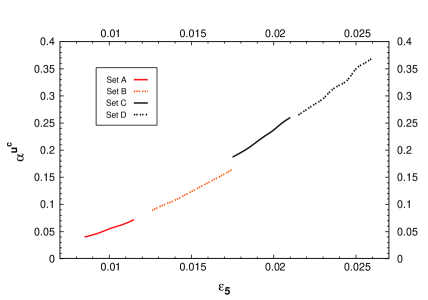
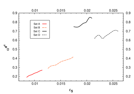
Figure 2: Correlation between the orbifold parameters ($\alpha^{u^{c}}$, $\varepsilon_{5}$) and ($\alpha^{d^{c}}$, $\varepsilon_{5}$), for distinct sets of input quark masses, A-D (red full lines, red dashed lines, full black and dashed black lines, respectively).

Rather than scatter plots, in Fig. 2 we present sets of points. This is due to having very narrow intervals of fluctuation for all the parameters. As an example, let us mention that for constant values of $\varepsilon_{5}$, $\alpha^{d^{c}}$ and $\beta^{f}$, $\alpha^{u^{c}}$ is fixed within a $2\%$ interval. ¿From Fig. 2 it is clear that for a given set of Higgs VEVs (determined by the associated set of input quark masses - Table 1) the allowed orbifold parameter space is very constrained. This is a direct consequence of the increasing accuracy in the experimental determination of the $V_{\text{CKM}}$. In each set (A–D), moving outside the displayed ranges would translate in violating the experimental bounds on (at least) one of the CKM matrix elements. Larger values of $\varepsilon_{5}$ would also (typically) be associated with an up-quark mass below the current accepted range. Regarding the values of $\beta^{f}$, these are constrained to be $\beta^{f}\approx 1$ throughout the allowed parameter space (cf. Eq. (12)). From the direct inspection of Fig. 2, together with the fact that $\beta^{f}\approx 1$, it appears that at least two regimes for $\alpha^{f}$ are present. For the up sector, one would suggest that the orbifold configuration is such that $\alpha^{u^{c}}$ is roughly $\mathcal{O}(\varepsilon_{5})$, so that one is faced with regime (a). The same would happen for sets A and B in the down sector, although sets C and D appear to favour a regime with $\alpha^{d^{c}}\sim 1$, thus suggesting regime (c).

Let us now aim at understanding the behaviour of both $\alpha^{u^{c},d^{c}}$ as a function of $\varepsilon_{5}$. In Ref. [25], several analytical relations for the CKM matrix elements as a function of $\{\varepsilon_{5},\alpha^{f},\beta^{f}\}$ were derived. Although those relations were computed for the case of hermitic mass matrices, where $V^{f}_{L}=V^{f}_{R}$, and are thus not truly valid for the present case, they are quite useful in understanding Fig. 2. For instance, the Cabibbo angle is given, to a very good approximation, by

$$V_{us}\approx-\varepsilon_{5}^{2}\left(\frac{m_{t}}{m_{c}}\,\frac{1}{\alpha^{u^{c}}}-\frac{m_{b}}{m_{s}}\,\frac{1}{\alpha^{d^{c}}}\right)\,,$$ (55)

and the above expression is clearly dominated by the first term on the right-hand side (r.h.s). From Eq. (55), it becomes transparent that the dependence of $\alpha^{u^{c}}$ on $\varepsilon_{5}$ should indeed be parabolic, as clearly displayed in Fig. 2. Regarding $\alpha^{d^{c}}$, its evolution is strongly influenced by the allowed regions of $\varepsilon_{5}$ (as dictated by the quark mass regimes taken as input, especially $m_{s}/m_{b}$). For sets A and B, the ratio of down-type quark masses is such that the leading term in the analytical expression of $V_{ub}$,

$$V_{ub} \approx\left(\frac{m_{s}}{m_{b}}\alpha^{d^{c}}-\frac{m_{c}}{m_{t}}\alpha^{u^{c}}\right)-\varepsilon_{5}\left(\frac{m_{d}}{m_{b}}\frac{m_{t}}{m_{c}}\frac{\alpha^{d^{c}}}{\alpha^{u^{c}}\beta^{d^{c}}}-\frac{m_{u}}{m_{t}}\frac{1}{\beta^{u^{c}}}\right)+\mathcal{O}(\varepsilon_{5}^{6})\,,$$ (56)

provides a reasonable understanding of $\alpha^{d^{c}}(\varepsilon_{5})$. For sets C and D, the situation is more involved, and the second term on the r.h.s. of Eq. (56) plays an important role. In fact, $\alpha^{d^{c}}$ receives contributions which display a near-resonant behaviour for the input quark mass ratios in the correspondent $\varepsilon_{5}$ range. This is the origin of the unexpected positioning of set C in Fig. 2.

We now address the behaviour of $a^{u^{c}}$ and $a^{d^{c}}$. By construction, and as clearly seen from Eq. (11), once $\varepsilon_{5}$ and $\alpha^{f}$ (or equivalently $\varepsilon_{5}$ and $\beta^{f}$) are set, one is implicitly fixing $a^{f}$. Moreover, satisfying the EWSB conditions for the VEVs, together with imposing a given value of $\tan\beta$ also translates in determining $g\,N$ and $\varepsilon_{1}$. In Fig. 3, we plot the values of $a^{u^{c}}$ and $a^{d^{c}}$ as a function of $\varepsilon_{5}$, as determined from Eq. (11).

Figure 3: Values of $a^{d^{c}}$ and $a^{u^{c}}$ (full and dashed lines, respectively) as a function of $\varepsilon_{5}$. Vertical dotted lines isolate the ranges of $\varepsilon_{5}$ associated with each set A-D.

As seen from Fig. 3, the behaviour of set C regarding $a^{d^{c}}$ is slightly misaligned with what one would expect from the analysis of sets A, B and D. Notice however that this is due to the dependence of $a^{d^{c}}$ on $\alpha^{d^{c}}$ (cf. Eq. (11)). Recall from Fig. 2 that for set C, the allowed values of $\alpha^{d^{c}}$ were somewhat higher than for the other cases, and this is the source of the suppression displayed in Fig. 3, set C.

In Fig. 4, we present the values of $\varepsilon_{1}$ as a function of $\varepsilon_{5}$ for the four sets of quark masses, and distinct regimes of $\tan\beta$.

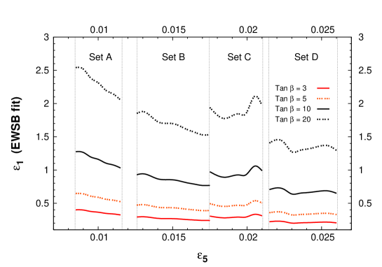
Figure 4: $\varepsilon_{1}$ as a function of $\varepsilon_{5}$ for $\tan\beta=$3, 5, 10 and 20 (red full lines, red dashed lines, full black and dashed black lines, respectively). Vertical dotted lines isolate the ranges of $\varepsilon_{5}$ associated with each set A-D.

¿From Fig. 4 we can also verify that the values of $\varepsilon_{1}$ are, in general, larger than those of $\varepsilon_{5}$. The “misaligned” behaviour of set C is again a consequence of the effects already discussed. Regarding the actual value of $g\,N$ it suffices to mention that for the orbifold parameter space here investigated, and for the values of $\tan\beta$ here selected, one has $1.03\,\lesssim g\,N\lesssim\,1.16$ .

Since we now have the relevant information, we can further compute the value of the lattice’s diagonal moduli, $T_{1}$ and $T_{5}$, as defined in Eq. (4). The value of $T_{5}$ is unambiguously determined. Nevertheless, and since the determination of $\varepsilon_{1}$ is a direct consequence of complying with the EWSB conditions for a fixed value of $\tan\beta$, its determination varies accordingly. In Fig. 5 we display the diagonal moduli as a function of $\varepsilon_{5}$, for $\tan\beta=$3, 5, 10 and 20.

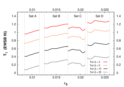
Figure 5: Diagonal lattice moduli, $T_{1}$ (left) and $T_{5}$ (right), as a function of $\varepsilon_{5}$. For the case of $T_{1}$, we plot it for several values of $\tan\beta=$3, 5, 10 and 20 (following the line and colour scheme of Fig. 4). For $T_{5}$ the dotted line denotes the prediction of the orbifold.

¿From Fig. 5, it is manifest that for the parameter space investigated, the values of the diagonal moduli, $T_{1}$ and $T_{5}$, are never degenerate. This confirms our original assumption (see footnote 2) that distinct moduli are indeed required to accommodate the experimental data. Although we have allowed for non-degenerate $T_{i}$, this remains quite a restrictive choice. We recall that we still have six additional degrees of freedom, namely the angles between the complex planes, which we have taken as zero in the present analysis.

To conclude the study of the orbifold parameter space, let us just plot the values of the Higgs VEVs, again as a function of $\varepsilon_{5}$. As an illustrative example, depicted in Fig. 6, we take $\tan\beta=5$.

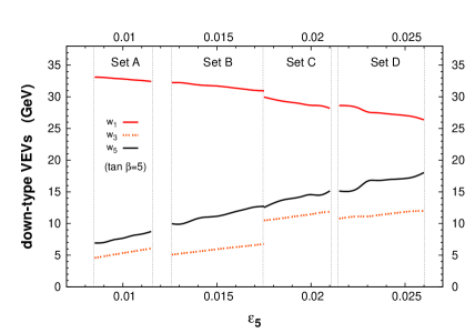
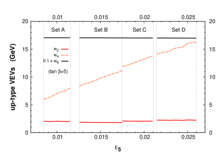
Figure 6: Down- and up-type Higgs VEVs, $w_{1,3,5}$ and $w_{2,4,6}$, as a function of $\varepsilon_{5}$, for $\tan\beta=$5. For convenience, we plot $w_{6}/10$. As before, vertical dotted lines isolate the ranges of $\varepsilon_{5}$ associated with each set A-D.

It is interesting to comment that in the up-sector, the VEVs exhibit a clearly hierarchical pattern, $w_{2}<w_{4}<w_{6}$ while in the down-type VEVs we encounter a not so definite pattern, with $w_{3}<w_{5}<w_{1}$. This is a direct consequence of the relations given in Eq. (2.2).

Finally, let us summarise our analysis of the orbifold parameter space by commenting on the relative number of input parameters and number of observables fitted. Working with the six Higgs VEVs ($w_{i}$), and the orbifold parameters $\varepsilon_{1}$, $\varepsilon_{5}$, $\alpha^{u^{c}}$ and $\alpha^{d^{c}}$, one can obtain the correct EWSB ($M_{Z}$), as well as the correct quark masses and mixings (six masses and three mixing angles).

5.2 Tree-level FCNCs in neutral mesons

The present orbifold model does not include a specific prediction regarding the Higgs sector. For instance, we have no hint regarding the value of the several bilinear terms, nor towards their origin. Concerning the soft breaking terms, the situation is identical. Since the FI $D$-term, which could have broken SUSY at the string scale, was cancelled, one must call upon some other mechanism to ensure that supersymmetry is indeed broken in the low-energy theory. In the absence of further information, we merely assume that the structure of the soft breaking terms is as in Eq. (36), taking the Higgs soft breaking masses and the $B\mu$-terms as free parameters (provided that the EW symmetry breaking and minimisation conditions are verified).

Before proceeding, it is important to stress that the Higgs spectrum (i.e. the scalar and pseudoscalar physical masses) cannot be a direct input when investigating the occurrence of FCNCs. In some previous studies of FCNCs in multi-Higgs doublets models (see for example [63]) the bounds were derived for the diagonal entries in the scalar and pseudoscalar mass matrices. However, this approach neglects mixings between the several fields $R_{i},I_{i}$, and excludes the exchange of some scalar and pseudoscalar states.

Although it is possible to begin the analysis from the original basis (where all neutral Higgses develop VEVs), we prefer to define the Higgs parameters on the Higgs-basis, relying on the minima conditions (and associated inequalities) to ensure that we are on the presence of true minima. Therefore, the parameters that must be specified are:

$$\tan\beta\,,\quad m^{2}_{ij}\,,\quad b_{ij}\,,$$ (57)

entering in Eq. (42). In the absence of orbifold predictions for the Higgs sector parameters, and motivated by an argument of simplicity, we begin our analysis by considering textures for the above parameters as simple as possible.

To avoid rewriting the Higgs soft-breaking masses, we adopt the following parameterisation:

$$m^{(d)}_{ij}=\left(\begin{array}[]{ccc}\otimes&\otimes&\otimes\\ \otimes&x_{3}&y\\ \otimes&y&x_{5}\end{array}\right)\times{1\text{TeV}}\,,\quad m^{(u)}_{kl}=\left(\begin{array}[]{ccc}\otimes&\otimes&\otimes\\ \otimes&x_{4}&y\\ \otimes&y&x_{6}\end{array}\right)\times{1\text{TeV}}\,,\quad\sqrt{b_{ij}}=b\times{1\text{TeV}}\,.$$ (58)

In the above, $m^{d(u)}$ should be understood as the $i,j=1,3,5$ ($k,l=2,4,6$) submatrices of the $6\times 6$ matrix that encodes the rotated soft-breaking Higgs masses in the Higgs basis (see [76]). The symbol $\otimes$ denotes an entry which is fixed by the minima equations of Eq. (42). This parametrisation allows to easily define the Higgs sector via six dimensionless parameters. We begin by taking a near-universality limit for the Higgs-sector textures introduced in Eq. (58). Regarding the value of $\tan\beta$, and if not otherwise stated, we shall take $\tan\beta=5$ in the subsequent analysis. We first consider the following four cases, presenting the associated scalar and pseudoscalar Higgs spectra:

• $x_{3}=x_{4}=0.5\,,x_{5}=x_{6}=0.75\,,y=0.1\,,b=0.1\,$

  $m^{s}=\{82.5,190.6,493.9,515.9,744.4,760.2\}$ GeV ;

  $m^{p}=\{186.8,493.9,515.9,744.4,760.2\}$ GeV .

• $x_{3}=x_{4}=0.4\,,x_{5}=x_{6}=0.8,y=0.15\,,b=0.2\,$

  $m^{s}=\{84.6,213.9,387.4,560.8,785.9,879.1\}$ GeV ;

  $m^{p}=\{215.2,387.3,560.5,785.9,878.9\}$ GeV .

• $x_{3}=x_{4}=0.75\,,x_{5}=x_{6}=1,y=0.25\,,b=0.2\,$

  $m^{s}=\{83.6,292.9,733.6,785.9,987.6,1057.0\}$ GeV ;

  $m^{p}=\{291.1,733.6,785.9,987.6,1057.0\}$ GeV .

• $x_{3}=x_{4}=0.3\,,x_{5}=x_{6}=0.8,y=0.1\,,b=0.1\,$

  $m^{s}=\{79.4,121.5,296.9,354.3,794.6,808.8\}$ GeV ;

  $m^{p}=\{114.8,296.9,353.7,794.6,808.8\}$ GeV .

In Fig. 7 we plot the ratio $\Delta m_{K}/(\Delta m_{K})_{\text{exp}}$ versus $\varepsilon_{5}$, for cases (a)-(d). We considered $\tan\beta=5$ and, since the other sets of input quark masses were in general associated to smaller FCNC effects, we take the quarks masses as in “set B” (Table 1). Once again, all the points displayed comply with the bounds from the CKM matrix.

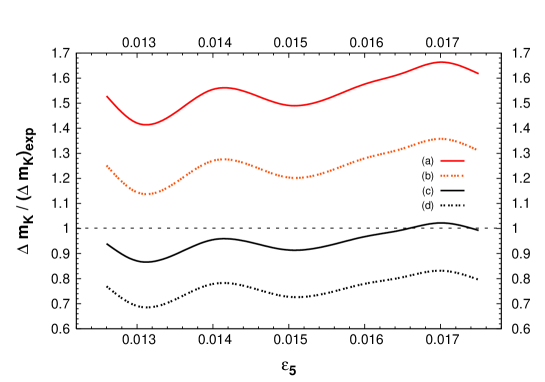
Figure 7: $\Delta m_{K}/(\Delta m_{K})_{\text{exp}}$ as a function of $\varepsilon_{5}$ for set B and $\tan\beta=5$. The Higgs parameters correspond to textures (a)-(d).

¿From Fig. 7 it is clear that it is quite easy for the orbifold model to accommodate the current experimental values for $\Delta m_{K}$. Even though the model presents the possibility of important tree-level contributions to the kaon mass difference, all the textures considered give rise to contributions very close to the experimental value. Although (a) and (b) are not in agreement with the measured value of $\Delta m_{K}$, their contribution is within order of magnitude of $(\Delta m_{K})_{\text{exp}}$. As seen from Fig. 7, with a considerably light Higgs spectrum (i.e. $m_{h^{0}_{i}}<1$ TeV), one is safely below the experimental bound, as exhibited by cases (c) and (d). This is not entirely unexpected given the strongly hierarchical structure of the Yukawa couplings (notice from Eq. (21) that $Y^{d}_{21}$ is suppressed by $\varepsilon_{5}^{2}$).

One important aspect clearly manifest in Fig. 7, and which has been overlooked in some previous analyses, is that the Higgs mixings can be as relevant as the Higgs eigenvalues in determining the contributions to $\Delta m_{K}$. This is patent in the comparison of curves (c) and (d). From a naïve inspection of the Higgs spectra associated to each case, one would expect that (c) would induce a much stronger suppression to the model’s contribution to $\Delta m_{K}$. Nevertheless, case (d), with a spectrum quite similar to case (b), and indeed much lighter than that of (d), but with much smaller mixings, is the one associated with the strongest suppression of $\Delta m_{K}$.

Figure 8: $\Delta m_{K}/(\Delta m_{K})_{\text{exp}}$ as a function of $\tan\beta$ for set B. The Higgs parameters correspond to texture (c).

It is also important to comment on the effect of changing $\tan\beta$ regarding the contributions to the kaon mass difference. For the specific case of texture (c), let us investigate the effect of varying $\tan\beta$. We take the quark masses as in set B, and while keeping the Higgs parameters fixed, $\tan\beta$ is taken in the range $3\lesssim\tan\beta\lesssim 9.5$. As it becomes clear from Fig. 8, larger values of $\tan\beta$ produce increasingly larger contributions to $\Delta m_{K}$. This is a direct consequence of the fact that, due to larger off-diagonal terms in the Higgs mass matrices, the mixing is larger, and the corresponding eigenstates become lighter. Even though the masses of the heaviest states remain stable, the intermediate states become lighter, and the FCNC contributions are less suppressed. Close to $\tan\beta$=10, it is no longer possible to find physical minima of the Higgs potential, and tachyonic states emerge. This effect has been already pointed out in the general analysis of [76].

5.2.1 $\boldsymbol{B_{d}}$ and $\boldsymbol{B_{s}}$ meson mass difference

For the several parameterisations of the Higgs sector used for the analysis of $\Delta m_{K}$, we display in Fig. 9 the contributions of Higgs textures (a)-(d) to the ${B_{d}}$ mass difference.

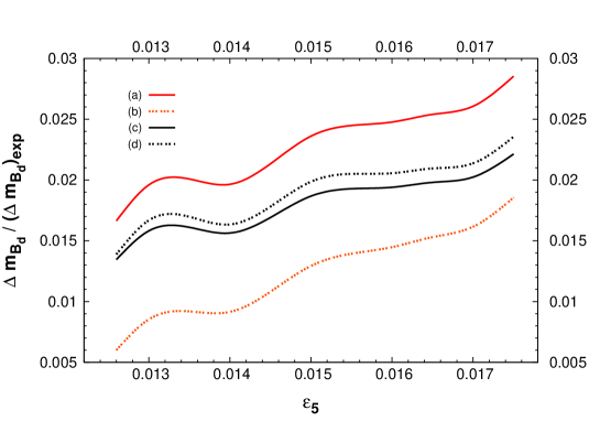
Figure 9: $\Delta m_{B_{d}}/(\Delta m_{B_{d}})_{\text{exp}}$ as a function of $\varepsilon_{5}$ for set B and $\tan\beta=5$. The Higgs parameters correspond to textures (a)-(d).

As one would expect, given the structure of the mass matrices (and thus the Yukawa couplings), the present model generates very small contributions to $\Delta m_{B_{d}}$. All the textures analysed, even those associated with excessive contributions to $\Delta m_{K}$ are in good agreement with the experimental data on the $B_{d}$ mass difference. Notice that the behaviour of the textures is now quite distinct: as an example, texture (b), which generated the second largest contribution to the $\Delta m_{K}$ is now the one associated with the strongest suppression. This stems from the fact that the leading contributions are now given by distinct Higgses, whose couplings to the quarks need not be identical.

Likewise, in Fig. 10 we plot the contributions to the ${B_{s}}$ mass difference. In this case experiment only provides a lower bound, so that any ratio larger than 1 is in agreement with current data.

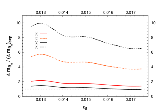
Figure 10: $\Delta m_{B_{s}}/(\Delta m_{B_{s}})_{\text{exp}}$ as a function of $\varepsilon_{5}$ for set B and $\tan\beta=5$. The Higgs parameters correspond to textures (a)-(d).

As we would expect from the discussion of Section 4, this model’s contributions to $\Delta m_{B_{s}}$ are well above the current limit.

5.2.2 $\boldsymbol{D^{0}-\bar{D}^{0}}$ mass difference

The cases (a)-(d) considered in the previous subsections generate contributions to $\Delta m_{D}$ that exceed the experimental bounds by at least a factor 10. As discussed in Section 4, this is not surprising, nor excessively worrying. Nevertheless, and for the sake of completing the analysis, let us consider four additional Higgs patterns, in order to derive a bound on the mass of the heaviest Higgs boson that would render the model compatible with the data from the $D^{0}$ sector.

The new Higgs textures are defined as follows:

• $x_{3}=x_{4}=0.75\,,x_{5}=2.5\,,x_{6}=7.5\,,y=0.5\,,b=0.5\,$

  $m^{s}=\{84.2,672.7,704.9,1414,2573,7501\}$ GeV ;

  $m^{p}=\{673.1,704.9,1414,2573,7501\}$ GeV .

• $x_{3}=x_{4}=0.5\,,x_{5}=5\,,x_{6}=7.5\,,y=0.5\,,b=0.1\,$

  $m^{s}=\{82.7,201.4,492.4,516.4,5000,7500\}$ GeV ;

  $m^{p}=\{197.9,492.4,516.4,5000,7500\}$ GeV .

• $x_{3}=x_{4}=1\,,x_{5}=x_{6}=7.5\,,y=0.5\,,b=0.5\,$

  $m^{s}=\{82.3,378.5,958.9,1578,7483,7518\}$ GeV ;

  $m^{p}=\{379.2,958.9,1578,7484,7518\}$ GeV .

• $x_{3}=x_{4}=3\,,x_{5}=x_{6}=7\,,y=1\,,b=0.5\,$

  $m^{s}=\{84.1,1032,2964,3059,6984,7022\}$ GeV ;

  $m^{p}=\{1031,2964,3059,6984,7022\}$ GeV .

For the cases (e) to (h) we present in Fig. 11 the contributions to $\Delta m_{D}$.

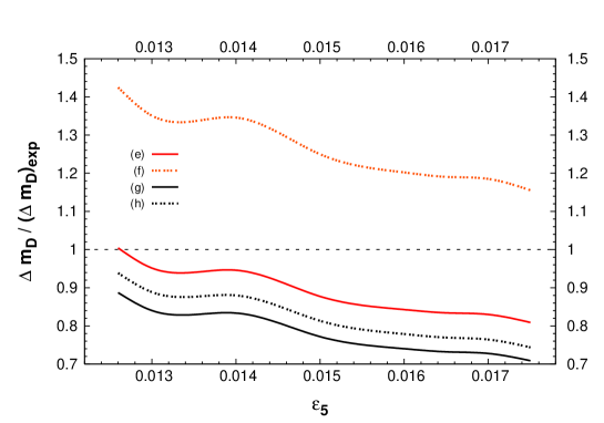
Figure 11: $\Delta m_{D}/(\Delta m_{D})_{\text{exp}}$ as a function of $\varepsilon_{5}$ for set B and $\tan\beta=5$. The Higgs parameters correspond to textures (e)-(h).

Compatibility with experiment can be obtained for any of the sets (e), (g) or (h), thus suggesting that one of the Higgses (a state mostly dominated by an up-type Higgs field) must be at least of around 7.5 TeV. Notice that no major hierarchy is required from the Higgs spectrum - case (e) is an excellent example of the latter statement, in the sense that one obtains states softly ranging from 600 to 7500 GeV. One may wonder if such a choice of Higgs soft-breaking terms may lead to a fine-tuning problem. In [76], it was pointed out that for non-degenerate VEVs, soft-breaking terms above the few TeV range typically induced a fine tuning stronger than 1%. Nevertheless, we again stress that these values for the Higgs masses (as derived from the $D^{0}$ mass difference analysis) should not be interpreted from a very strict point of view.

5.3 Tree-level CP violation: $\boldsymbol{\varepsilon_{K}}$

Finally, we turn our attention to the issue of CP violation. So far, we have seen that accommodating the several $\Delta F=2$ observables is not an excessively hard task (especially if we choose to set aside the $D^{0}$ sector). Nevertheless, a successful model of particle physics must also comply with the observed CP violation in the kaon sector. As we mentioned in Section 4, we will only consider the specific contribution of the present model to indirect CP violation in the kaon sector ($\varepsilon_{K}$). Therefore, we now assume $\varepsilon_{5}$ (and thus $\alpha^{f}$) to be a complex quantity, and parameterise it as $\varepsilon_{5}=|\varepsilon_{5}|\,e^{i\phi}$.

In Fig. 12 we present the tree-level contributions to $\varepsilon_{K}$ (normalised by its experimental value) as a function of $|\varepsilon_{5}|$. We take the input quark masses as in set B, fix $\tan\beta=5$, and analyse the Higgs textures associated with cases (c), (d) and (e). For each texture, the phase is assumed to be $\phi_{c}=4.0\times 10^{-4}$, $\phi_{d}=2.5\times 10^{-4}$ and $\phi_{e}=2.5\times 10^{-3}$. These phases are taken as illustrative examples; we choose values that for a specific set of input quark masses (set B, in this case) and a given Higgs texture (c)-(e) simultaneously succeed in generating an amount of $\varepsilon_{K}$ close to the value experimentally measured (range delimited by dotted grey lines in Fig. 12), and still have a compatible CKM. One should bare in mind that once $\arg\varepsilon_{5}$ (and thus $\arg\alpha^{f}$) is no longer a small number, it will significantly affect the computation of the Yukawa couplings, and thus the CKM matrix.

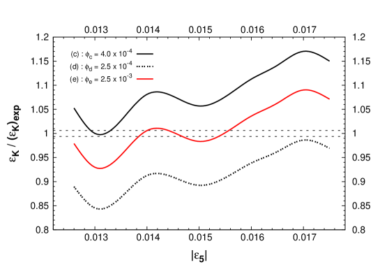
Figure 12: $\varepsilon_{K}/(\varepsilon_{K})_{\text{exp}}$ as a function of $|\varepsilon_{5}|$ for set B and $\tan\beta=5$. The Higgs parameters correspond to textures (c)-(e).

We have considered one texture that accommodates all FCNC observables, namely texture (e), which already has a somewhat heavy Higgs spectrum. In this case, the phase required to saturate $(\varepsilon_{K})_{\text{exp}}$ is $\mathcal{O}(10^{-3})$. Since we do not wish to view the $D^{0}$ sector as a very stringent constraint, we also consider two other Higgs patterns, (c) and (d), which only succeed in complying with both kaon and $B$-meson data. In these cases, the phases necessary to obtain $(\varepsilon_{K})_{\text{exp}}$ are now $\mathcal{O}(10^{-4})$, as one would expect, since a lighter set of Higgs bosons typically enhances the contributions.

In the range of parameters analysed in this plot, the amount of CP violation stemming from the CKM matrix is $J_{CP}\sim\mathcal{O}(10^{-8}-10^{-6})$, i.e. at least one order of magnitude below the SM value that is associated with the observed $\varepsilon_{K}$ [1]. The possibility of obtaining an orbifold configuration that saturates the observed value of $\varepsilon_{K}$ and at the same time allows to reproduce the $J_{CP}$ required by the unitarity triangle fits should not be discarded. It is clear that the phase of $\varepsilon_{5}$ must be quite large, and such values would push us to distinct areas of the orbifold parameter space. It is worth emphasising that there are still other sources of CP violation in addition to the one we have studied in this Section. As mentioned in footnote 3, a more complicated choice of the VEVs $c_{i}$ could lead to physical phases in the quark masses matrices, which would in turn contribute to the physical CKM phase.

6 Conclusions

In this work we have investigated whether it is possible to find abelian $Z_{3}$ orbifold configurations that are associated with an experimentally viable low-energy scenario.

This class of models provides a beautiful geometric mechanism for the generation of the fermion mass hierarchy. The Yukawa couplings are explicitly calculable, and thus a solution to the elusive flavour problem of the SM and MSSM can in principle be obtained.

We have concentrated here in $Z_{3}$ orbifold compactifications with two Wilson lines, which naturally include three families for fermions and Higgses. The fact that additional Yukawas are present opens the possibility of obtaining realistic fermion masses and mixings, entirely at the renormalisable level (with a key role being played by the FI breaking). We have surveyed the parameter space generated by the free orbifold parameters, and we have verified that one can find configurations that obey the EW symmetry breaking conditions, and can account for the correct quark masses and mixings.

On the other hand, having six Higgs doublets (and thus six quark Yukawa couplings) poses the potential problem of having tree-level FCNCs. By assuming simple textures for the Higgs free parameters, we have verified that the experimental data on the neutral kaon mass difference, as well as on $\Delta m_{B_{d}}$ and $\Delta m_{B_{s}}$ can be easily accommodated for a quite light Higgs spectra, namely $m_{h^{0}_{i}}\lesssim 1$ TeV. The data from the $D^{0}$ sector proves to be a more difficult challenge, requiring a Higgs spectrum of at least 7 TeV, but we again stress that, in view of the theoretical and experimental uncertainties associated with the $D^{0}$ sector, this constraint should not be over-emphasised.

CP violation can be also embedded into the low-energy theory. Although CP is a gauge symmetry of the full theory, it can be spontaneously broken at the string scale, if the VEVs of the moduli have a non-vanishing phase. We have parameterised these effects by assuming the presence of a phase in $\varepsilon_{5}$, and we have verified that one can also obtain a value for $\varepsilon_{K}$ in agreement with current experimental data.

The presence of a fairly light Higgs spectrum, composed by a total of 21 physical states, may provide abundant experimental signatures at future colliders, like the Tevatron or the LHC. In fact, flavour violating decays of the form $h_{i}\to q\bar{q}$, or $h_{i}\to l^{+}l^{-}$ may provide the first clear evidence of this class of models. $Z_{3}$ orbifold compactifications with two Wilson lines are equally predictive regarding the lepton sector. This analysis, especially that of the neutrino sector, will be addressed in a forthcoming work [77].

References

- [1] S. Eidelman et al. [Particle Data Group Collaboration], “Review of particle physics”, Phys. Lett. B 592 (2004) 1.
- [2] M. Maltoni, T. Schwetz, M. A. Tortola and J. W. F. Valle, “Status of global fits to neutrino oscillations”, New J. Phys. 6 (2004) 122 [arXiv:hep-ph/0405172].
- [3] A. Strumia and F. Vissani, “Implications of neutrino data circa 2005”, Nucl. Phys. B 726 (2005) 294 [arXiv:hep-ph/0503246].
- [4] G. L. Fogli, E. Lisi, A. Marrone and A. Palazzo, “Global analysis of three-flavor neutrino masses and mixings”, arXiv:hep-ph/0506083.
- [5] D. J. Gross, J. A. Harvey, E. J. Martinec and R. Rohm, “The heterotic string”, Phys. Rev. Lett. 54 (1985) 502; “Heterotic string theory. 1. The free heterotic string”, Nucl. Phys. B 256 (1985) 253; “Heterotic string theory. 2. The interacting heterotic string”, Nucl. Phys. B 267 (1986) 75.
- [6] L. J. Dixon, J. A. Harvey, C. Vafa and E. Witten, “Strings on orbifolds. 1”, Nucl. Phys. B 261 (1985) 678; “Strings on orbifolds. 2”, Nucl. Phys. B 274 (1986) 285.
- [7] L. E. Ibáñez, H. P. Nilles and F. Quevedo, “Orbifolds and Wilson lines”, Phys. Lett. B 187 (1987) 25.
- [8] L. E. Ibáñez, J. E. Kim, H. P. Nilles and F. Quevedo, “Orbifold compactifications with three families of ”, Phys. Lett. B 191 (1987) 282.
- [9] D. Bailin, A. Love and S. Thomas, “A three generation orbifold compactified superstring model with realistic gauge group”, Phys. Lett. B 194 (1987) 385.
- [10] L. E. Ibáñez, J. Mas, H. P. Nilles and F. Quevedo, “Heterotic strings in symmetric and asymmetric orbifold backgrounds”, Nucl. Phys. B 301 (1988) 157.
- [11] J. A. Casas, E. K. Katehou and C. Muñoz, “U(1) charges in orbifolds: anomaly cancellation and phenomenological consequences”, Nucl. Phys. B 317 (1989) 171.
- [12] A. Font, L. E. Ibáñez, H. P. Nilles and F. Quevedo, “Degenerate orbifolds”, Nucl. Phys. B 310 (1988) 109.
- [13] J. E. Kim, “The strong CP problem in orbifold compactifications and an model”, Phys. Lett. B 207 (1988) 434.
- [14] J. A. Casas and C. Muñoz, “Three generation orbifold models through Fayet-Iliopoulos terms”, Phys. Lett. B 209 (1988) 214.
- [15] J. A. Casas and C. Muñoz, “Three generation models from orbifolds”, Phys. Lett. B 214 (1988) 63.
- [16] A. Font, L. E. Ibáñez, H. P. Nilles and F. Quevedo, “Yukawa couplings in degenerate orbifolds: towards a realistic superstring”, Phys. Lett. B 210 (1988) 101 [Erratum-ibid. B 213 (1988) 564].
- [17] J. A. Casas and C. Muñoz, “Yukawa couplings in orbifold models”, Phys. Lett. B 212 (1988) 343.
- [18] J. A. Casas and C. Muñoz, “Restrictions on realistic superstring models from renormalization group equations”, Phys. Lett. B 214 (1988) 543.
- [19] A. Font, L. E. Ibáñez, F. Quevedo and A. Sierra, “The construction of ’realistic’ four-dimensional strings through orbifolds”, Nucl. Phys. B 331 (1990) 421.
- [20] J. A. Casas M. Mondragon and C. Muñoz, “Reducing the number of candidates to standard model in the orbifold”, Phys. Lett. B 230 (1989) 63.
- [21] Y. Katsuki, Y. Kawamura, T. Kobayashi, N. Ohtsubo, Y. Ono and K. Tanioka, “Z(N) orbifold models”, Nucl. Phys. B 341 (1990) 611.
- [22] H. B. Kim and J. E. Kim, “An orbifold compactification with three families from twisted sectors”, Phys. Lett. B 300 (1993) 343 [arXiv:hep-ph/9212311].
- [23] G. Aldazabal, A. Font, L. E. Ibáñez and A. M. Uranga, “Building GUTs from strings”, Nucl. Phys. B 341 (1990) 611 [arXiv:hep-th/9508033].
- [24] C. Muñoz, “A kind of prediction from superstring model building”, JHEP 0112 (2001) 015 [arXiv:hep-ph/0110381].
- [25] S. A. Abel and C. Muñoz, “Quark and lepton masses and mixing angles from superstring constructions”, JHEP 0302 (2003) 010 [arXiv:hep-ph/0212258].
- [26] T. Kobayashi, S. Raby and R. J. Zhang, “Searching for realistic 4d string models with a Pati-Salam symmetry: Orbifold grand unified theories from heterotic string compactification on a Z(6) orbifold”, Nucl. Phys. B 704 (2005) 3 [arXiv:hep-ph/0409098].
- [27] T. Kobayashi and C. Muñoz, “More about soft terms and FCNC in realistic string constructions”, arXiv:hep-ph/0508286.
- [28] W. Buchmuller, K. Hamaguchi, O. Lebedev and M. Ratz, “The supersymmetric standard model from the heterotic string”, arXiv:hep-ph/0511035.
- [29] P. Candelas, G. T. Horowitz, A. Strominger and E. Witten, “Vacuum configurations for superstrings”, Nucl. Phys. B 258 (1985) 46.
- [30] H. Kawai, D. C. Lewellen and S. H. H. Tye, “Construction of four-dimensional fermionic string models”, Phys. Rev. Lett. 57 (1986) 1832 [Erratum-ibid. 58 (1987) 429]; “Construction of fermionic string models in four-dimensions”, Nucl. Phys. B 288 (1987) 1.
- [31] I. Antoniadis, C. P. Bachas and C. Kounnas, “Four-dimensional superstrings”, Nucl. Phys. B 289 (1987) 87.
- [32] P. Horava and E. Witten, “Heterotic and type I string dynamics from eleven dimensions”, Nucl. Phys. B 460 (1996) 506 [arXiv:hep-th/9510209]; “Eleven-dimensional supergravity on a manifold with boundary”, Nucl. Phys. B 475 (1996) 94 [arXiv:hep-th/9603142].
- [33] E. Witten, Nucl. Phys. B 471 (1996) 135 [arXiv:hep-th/9602070].
- [34] B. R. Greene, K. H. Kirklin, P. J. Miron and G. G. Ross, “A superstring inspired standard model”, Phys. Lett. B 180 (1986) 69; “A three generation superstring model. 1. Compactification and discrete symmetries”, Nucl. Phys. B 278 (1986) 667; “A three generation superstring model. 2. Symmetry breaking and the low-energy theory”, Nucl. Phys. B 292 (1987) 606.
- [35] R. Donagi, Y. H. He, B. A. Ovrut and R. Reinbacher, “The spectra of heterotic standard model vacua”, JHEP 0506 (2005) 070 [arXiv:hep-th/0411156].
- [36] V. Braun, Y. H. He, B. A. Ovrut and T. Pantev, “A heterotic standard model”, Phys. Lett. B 618 (2005) 252 [arXiv:hep-th/0501070]; “A standard model from the E(8) x E(8) heterotic superstring”, JHEP 0506 (2005) 039 [arXiv:hep-th/0502155]; “The exact MSSM spectrum from string theory”, arXiv:hep-th/0512177.
- [37] I. Antoniadis, J. R. Ellis, J. S. Hagelin and D. V. Nanopoulos, “GUT model building with fermionic four-dimensional strings”, Phys. Lett. B 205 (1988) 459; “An improved SU(5) X U(1) model from four-dimensional string”, Phys. Lett. B 208 (1988) 209 [Addendum-ibid. B 213 (1988) 562]; “The flipped SU(5) X U(1) string model revamped”, Phys. Lett. B 231 (1989) 65.
- [38] A. E. Faraggi, D. V. Nanopoulos and K. Yuan, “A standard like model in the 4-d free fermionic string formulation”, Nucl. Phys. B 335 (1990) 347.
- [39] G. B. Cleaver, A. E. Faraggi and D. V. Nanopoulos, “String derived MSSM and M-theory unification”, Phys. Lett. B 455 (1999) 135 [arXiv:hep-ph/9811427].
- [40] G. B. Cleaver, A. E. Faraggi, D. V. Nanopoulos and J. W. Walker, “Phenomenology of non-Abelian flat directions in a minimal superstring standard model”, Nucl. Phys. B 620 (2002) 259 [arXiv:hep-ph/0104091].
- [41] S. Chaudhuri, S. W. Chung, G. Hockney and J. D. Lykken, “String consistency for unified model building”, Nucl. Phys. B 456 (1995) 89 [arXiv:hep-ph/9501361].
- [42] S. Chaudhuri, G. Hockney and J. D. Lykken, “Three Generations in the Fermionic Construction”, Nucl. Phys. B 469 (1996) 357 [arXiv:hep-th/9510241].
- [43] R. Donagi, B. A. Ovrut, T. Pantev and D. Waldram, “Standard models from heterotic M-theory”, Adv. Theor. Math. Phys. 5, 93 (2002) [arXiv:hep-th/9912208].
- [44] E. Witten, “Some properties of O(32) superstrings”, Phys. Lett. B 149 (1984) 351.
- [45] M. Dine, N. Seiberg and E. Witten, “Fayet-Iliopoulos terms in string theory”, Nucl. Phys. B 289 (1987) 589.
- [46] J. J. Atick, L. J. Dixon and A. Sen, “String calculation of Fayet-Iliopoulos D terms in arbitrary supersymmetric compactifications”, Nucl. Phys. B 292 (1987) 109.
- [47] M. Dine, I. Ichinose and N. Seiberg, “F terms and D terms in string theory”, Nucl. Phys. B 293 (1987) 253.
- [48] S. Hamidi and C. Vafa, “Interactions on orbifolds”, Nucl. Phys. B 279 (1987) 465.
- [49] L. J. Dixon, D. Friedan, E. J. Martinec and S. H. Shenker, “The conformal field theory of orbifolds”, Nucl. Phys. B 282 (1987) 13.
- [50] L. E. Ibáñez, “Hierarchy of quark-lepton masses in orbifold superstring compactification”, Phys. Lett. B 181 (1986) 269.
- [51] J. A. Casas and C. Muñoz, “Fermion masses and mixing angles: a test for string vacua”, Nucl. Phys. B 332 (1990) 189 [Erratum-ibid. B 340 (1990) 280].
- [52] J. A. Casas, F. Gómez and C. Muñoz, “Fitting the quark and lepton masses in string theories”, Phys. Lett. B 292 (1992) 42 [arXiv:hep-th/9206083].
- [53] J. A. Casas, F. Gómez and C. Muñoz, “World sheet instanton contribution to Z(7) Yukawa couplings”, Phys. Lett. B 251 (1990) 99.
- [54] T. T. Burwick, R. K. Kaiser and H. F. Muller, “General Yukawa couplings of strings on Z(N) orbifolds”, Nucl. Phys. B 355 (1991) 689.
- [55] T. Kobayashi and N. Ohtsubo, “Geometrical aspects of Z(N) orbifold phenomenology”, Int. J. Mod. Phys. A 9 (1994) 87.
- [56] J. A. Casas, F. Gómez and C. Muñoz, “Complete structure of Z(n) Yukawa couplings,” Int. J. Mod. Phys. A 8 (1993) 455 [arXiv:hep-th/9110060].
- [57] P. Ko, T. Kobayashi and J. h. Park, “Quark masses and mixing angles in heterotic orbifold models”, Phys. Lett. B 598 (2004) 263 [arXiv:hep-ph/0406041].
- [58] P. Ko, T. Kobayashi and J. h. Park, “Lepton masses and mixing angles from heterotic orbifold models”, Phys. Rev. D 71 (2005) 095010 [arXiv:hep-ph/0503029].
- [59] H. Georgi and D. V. Nanopoulos, “Suppression of flavor changing effects from neutral spinless meson exchange in gauge theories”, Phys. Lett. B 82 (1979) 95.
- [60] B. McWilliams and L. F. Li, “Virtual effects of Higgs particles”, Nucl. Phys. B 179 (1981) 62.
- [61] O. Shanker, “Flavor violation, scalar particles and leptoquarks”, Nucl. Phys. B 206 (1982) 253.
- [62] R. A. Flores and M. Sher, “Higgs masses in the standard, multi-Higgs and supersymmetric models”, Annals Phys. 148 (1983) 95.
- [63] T. P. Cheng and M. Sher, “Mass matrix ansatz and flavor nonconservation in models with multiple Higgs doublets”, Phys. Rev. D 35 (1987) 3484.
- [64] J. R. Ellis, D. V. Nanopoulos, S. T. Petcov and F. Zwirner, “Gauginos and Higgs particles in superstring models”, Nucl. Phys. B 283 (1987) 93.
- [65] M. Drees, “Supersymmetric models with extended Higgs sector,” Int. J. Mod. Phys. A 4 (1989) 3635.
- [66] K. Griest and M. Sher, “Phenomenology and cosmology of extra generations of Higgs bosons”, Phys. Rev. Lett. 64 (1990) 135.
- [67] K. Griest and M. Sher, “Phenomenology and cosmology of second and third family Higgs bosons”, Phys. Rev. D 42 (1990) 3834.
- [68] H. E. Haber and Y. Nir, “Multiscalar models with a high-energy scale”, Nucl. Phys. B 335 (1990) 363.
- [69] M. Sher and Y. Yuan, “Rare B decays, rare tau decays and grand unification”, Phys. Rev. D 44 (1991) 1461.
- [70] N. V. Krasnikov, “Electroweak model with a Higgs democracy”, Phys. Lett. B 276 (1992) 127.
- [71] A. Antaramian, L. J. Hall and A. Rasin, “Flavor changing interactions mediated by scalars at the weak scale”, Phys. Rev. Lett. 69 (1992) 1871 [arXiv:hep-ph/9206205].
- [72] A. E. Nelson and L. Randall, “Naturally large tan beta”, Phys. Lett. B 316 (1993) 516 [arXiv:hep-ph/9308277].
- [73] M. Masip and A. Rasin, “Spontaneous CP violation in supersymmetric models with four Higgs doublets”, Phys. Rev. D 52 (1995) 3768 [arXiv:hep-ph/9506471].
- [74] M. Masip and A. Rasin, “CP violation in multi-Higgs supersymmetric models”, Nucl. Phys. B 460 (1996) 449 [arXiv:hep-ph/9508365].
- [75] A. Aranda and M. Sher, “Generations of Higgs bosons in supersymmetric models”, Phys. Rev. D 62 (2000) 092002 [arXiv:hep-ph/0005113].
- [76] N. Escudero, C. Muñoz and A. M. Teixeira, “FCNCs in supersymmetric multi-Higgs doublet models”, arXiv:hep-ph/0512046.
- [77] N. Escudero, F. R. Joaquim, C. Muñoz and A. M. Teixeira, work in progress.
- [78] J. Giedt, “The KM phase in semi-realistic heterotic orbifold models”, Nucl. Phys. B 595 (2001) 3 [Erratum-ibid. B 632 (2002) 397] [arXiv:hep-ph/0007193]; “CP violation and moduli stabilization in heterotic models”, Mod. Phys. Lett. A 17 (2002) 1465 [arXiv:hep-ph/0204017].
- [79] B. Acharya, D. Bailin, A. Love, W. A. Sabra and S. Thomas, “Spontaneous breaking of CP symmetry by orbifold moduli”, Phys. Lett. B 357(1995) 387 [arXiv:hep-th/9506143].
- [80] D. Bailin, G. V. Kraniotis and A. Love, “CP-violating phases in the CKM matrix in orbifold compactifications”, Phys. Lett. B 435 (1998) 323 [arXiv:hep-th/9805111].
- [81] G. F. Giudice and A. Masiero, “A natural solution to the mu problem in supergravity theories”, Phys. Lett. B 206 (1988) 480.
- [82] G. Lopes Cardoso, D. Lüst and T. Mohaupt, “Moduli spaces and target space duality symmetries in (0,2) Z(N) orbifold theories with continuous Wilson lines”, Nucl. Phys. B 432 (1994) 68 [arXiv:hep-th/9405002].
- [83] I. Antoniadis, E. Gava, K. S. Narain and T. R. Taylor, “Effective mu term in superstring theory”, Nucl. Phys. B 432 (1994) 187 [arXiv:hep-th/9405024].
- [84] G. Burdman, “Potential for discoveries in charm meson physics”, arXiv:hep-ph/9508349.
- [85] S. Béjar, J. Guasch and J. Solà, “Production and FCNC decay of supersymmetric Higgs bosons into heavy quarks in the LHC”, JHEP 0510 (2005) 113 [arXiv:hep-ph/0508043].
- [86] A. M. Curiel, M. J. Herrero, W. Hollik, F. Merz and S. Peñaranda, “SUSY - electroweak one-loop contributions to flavour-changing Higgs-boson decays”, Phys. Rev. D 69 (2004) 075009 [arXiv:hep-ph/0312135].
- [87] J. A. Aguilar-Saavedra, “Top flavour-changing neutral interactions: Theoretical expectations and experimental detection”, Acta Phys. Polon. B 35 (2004) 2695 [arXiv:hep-ph/0409342].
- [88] C. Jarlskog, “Commutator of the quark mass matrices in the standard electroweak model and a measure of maximal CP violation”, Phys. Rev. Lett. 55 (1985) 1039; “A basis independent formulation of the connection between quark mass matrices, CP violation and experiment”, Z. Phys. C 29 (1985) 491.