Moments of Wigner function and Renyi entropies at freeze-out

Abstract

Relation between Renyi entropies and moments of the Wigner function, representing the quantum mechanical description of the M-particle semi-inclusive distribution at freeze-out, is investigated. It is shown that in the limit of infinite volume of the system, the classical and quantum descriptions are equivalent. Finite volume corrections are derived and shown to be small for systems encountered in relativistic heavy ion collisions.

1 Introduction

It is widely recognized that information on the entropy of the systems produced in high-energy collisions is very useful in understanding the physics of the process in question. This is particularly important for heavy ion collisions and search for quark-gluon plasma. It was suggested some time ago [1] that measurements of coincidences between the events observed in high-energy experiments may provide an estimate of the Renyi entropies [2] of the final state and thus also access information on its thermodynamical (Shannon) entropy. Although the idea seems attractive, the argument of [1], being essentially of classical nature, can only be considered as a first step. The proper formulation must take into account the quantum-mechanical nature of the problem. In the present paper a quantum-mechanical formulation is developed and its consequences discussed. In particular, it is shown that the classical approach of [1] is valid in the limit of very large size of the system in configuration space. For systems of finite size, quantum corrections are derived and shown to be relatively small for final states occuring in relativistic heavy ion collisions.

The order $l$ Renyi entropy, $H(l)$, of a statistical system is defined as

$$H(l)=\frac{1}{1-l}\log C(l),$$ (1)

where $C(l)$ are coincidence probabilities of the states of the system, given by

$$C(l)\equiv\sum_{i}[P_{i}]^{l}=Tr[\rho]^{l}.$$ (2)

The sum runs over all states of the system, $P_{i}$ is the probability of a state $i$ to occur and $\rho$ is the density matrix of the system.

The attractive property of Renyi entropies is their relation to the standard (Shannon) entropy of the statistical system. It is easy to show that

$$S\equiv Tr[\rho\log\rho]=\lim_{l\rightarrow 1}H(l),$$ (3)

where $S$ is the Shannon entropy.

Moreover since, as is well known [3], for $l\geq 1$

$$S\geq H(l)\geq H(l+1),$$ (4)

the Renyi entropies provide an exact lower limit for $S$, a quantity very important for understanding the properties of the quark-gluon plasma [4].

The object of our investigation is an M-particle statistical system, i.e., a collection of M-particle final states which we define as those in which exactly $M$ particles were observed in a given region of the momentum space. We shall call them $M$-particle events (independently of how many particles were actually produced).

On the classical level, M-particle final states can be described by the normalized $M$ particle phase-space distribution $W^{class}(X,K)$ with $X=X_{1},...,Z_{M}$, $K=K^{(1)}_{x},...,K^{(M)}_{z}$.

To obtain a quantum mechanical generalization of the phase-space distribution we follow the standard procedure, where the proper quantum description of an M-particle final state is given by the density matrix $\rho(p_{1},...,p_{M};p_{1}^{\prime},...,p_{M}^{\prime})$. As shown by Wigner [7] the quantum-mechanical analogue of the classical phase-space distribution (called Wigner function), can be defined in terms of the density matrix as the Fourier transform

$$W(X,K)=\frac{1}{(2\pi)^{3M}}\int dqe^{-iqX}\rho(p,p^{\prime}),$$ (5)

where $K=(p+p^{\prime})/2;\;q=p-p^{\prime}$. The quantum-mechanical description of multiparticle events is obtained by considering the Wigner function $W(X,K)$ instead of the classical phase-space distribution $W^{class}(X,K)$.

The main goal of this paper is to discuss the relation between the coincidence probabilities $C(l)$ defined in (2) and the moments of the Wigner function

$$\hat{C}(l)=(2\pi)^{3M(l-1)}\int d^{3M}X\int d^{3M}K[W(X,K)]^{l}.$$ (6)

Such a relation exists because both $C(l)$ and $\hat{C}(l)$ are defined in terms of the density matrix.

The factor $(2\pi)^{3M(l-1)}$ is introduced in (6) to account for the factor $(2\pi)^{-3M}$ in (5) (which insures consistency between the proper normalization of the density matrix and of the Wigner function). This choice guarantees that, when $W(X,K)$ in (6) is replaced by the classical density distribution $W^{class}(X,K)$, $\hat{C}(l)$ reproduces the correct classical limit of the coincidence probability, thus satisfying an important consistency constraint. We have

$$\hat{C}(l)\rightarrow C^{class}(l)\equiv\int d^{3M}Xd^{3M}KW^{class}(X,K)\left[(2\pi)^{3M}W^{class}(X,K)\right]^{l-1}.$$ (7)

In this formula $W^{class}(X,K)$ can be interpreted as probability distribution and $(2\pi)^{3M}W^{class}(X,K)$ as the probability for the system to occupy the elementary phase-space cell $(2\pi\hbar)^{3M}$ around the (6M-dimensional) point $(X,K)$. Thus one sees that, indeed, (7) represents the classical formula for the coincidence probability.

The interest in the relation between $\hat{C}(l)$ and $C(l)$ stems from the observation that the moments $\hat{C}(l)$ are experimentally accessible: we have shown recently [8] that, for a rather large class of models, $\hat{C}(l)$ defined above can be estimated from the measured coincidence probability $C^{exp}(l)$ of the events with $M$ particles [1, 9, 10]

$$C^{exp}(l)=\frac{N_{l}}{N(N-1)...(N-l+1)/l!},$$ (8)

where $N_{l}$ is the number of the observed l-plets of identical events and $N$ is the total number of events. $N(N-1)...(N-l+1)/l!$ is the total number of l-plets of events. One sees that measurement of $C^{exp}(l)$ reduces to counting the coincidence between observed events.

We show in this paper that $\hat{C}(l)$ (which can be measured by counting the number of identical events [8]), and $C(l)$ (which determine Renyi entropies and thus open a window to the true entropy) are equal in the limit of infinite size of the system. Also the finite volume (quantum) corrections are studied and shown to fall with inverse square of the smallest (linear) size.

In the next section a model for the Wigner function is introduced and the corresponding formulae for the moments $\hat{C}(l)$ are written down. In Section 3 the results of [8] are summarized. In Section 4 the coincidence probabilities $C(l)$ are analyzed in the same framework. The relation between $\hat{C}(l)$ and $C(l)$ are discussed in Section 5. Our conclusions and outlook are given in the last section.

2 Moments of the Wigner function

In terms of the Wigner function $W(K,X)$, the momentum distribution is given by the integral

$$w(K)\equiv e^{-v(K)}=\int d^{3M}XW(X,K).$$ (9)

To discuss $\hat{C}(l)$, we follow the argument of [8] and consider the time-averaged Wigner function of the rather general form, valid in a large variety of models [13]:

$$W(X,K)=\frac{1}{(L_{x}L_{y}L_{z})^{M}}G[X/L]w(K)$$ (10)

with $X/L\equiv(X_{1}-\bar{X}_{1})/L_{x},...,(Z_{M}-\bar{Z}_{M})/L_{z}$, $K=K_{1},...,K_{M}$. The function $G$ satisfies the normalization conditions

$$\int G(u)d^{3M}u = 1\;\;\rightarrow\;\;\int dXG(X/L)=(L_{x}L_{y}L_{z})^{M};$$

$$\int u_{i}G(u)d^{3M}u = 0\;\;\rightarrow\;\;<X_{i},Y_{i},Z_{i}>=\bar{X}_{i},\bar{Y}_{i},\bar{Z}_{i};$$

$$\int(u_{i})^{2}G(u)d^{3M}u = 1\;\;\rightarrow\;\;<(X_{i}-\bar{X}_{i})^{2},...>=L_{x}^{2},...$$ (11)

The first condition insures that $w(K)$ is the correctly normalized (multidimensional) momentum distribution, the second defines the central values of the particle distribution in configuration space and the third defines $L_{x},L_{y},L_{z}$ as root mean square sizes of the distribution in configuration space. Both sizes and central positions may depend on the particle momenta. The form of function $G$ is responsible for the shape of the multiparticle distribution in configuration space.

Using (10) we obtain from (6)

$$\hat{C}(l)=(2\pi)^{3M(l-1)}\int d^{3M}K[w(K_{1},...,K_{M})]^{l}\int\frac{d^{3M}X}{(L_{x}L_{y}L_{z})^{lM}}[G(X/L)]^{l}=$$

$$=(2\pi g_{l})^{3M(l-1)}\int d^{3M}K\frac{[w(K_{1},...,K_{M})]^{l}}{(L_{x}L_{y}L_{z})^{(l-1)M}}$$ (12)

with

$$(g_{l})^{3M(l-1)}=\int d^{3M}u[G(u)]^{l}$$ (13)

The constant $g_{l}$ depends on the shape of particle distribution in configuration space. For example, we obtain $(g_{l})^{-1}=\sqrt{2\pi}l^{1/[2(l-1)]}$ for Gaussians and $(g_{l})^{-1}=2\sqrt{3}$ for a rectangular box. In the following we shall assume that $G(u)$ is a Gaussian

$$G(u)=\frac{1}{(2\pi)^{3M/2}}e^{-\sum_{m=1}^{M}\sum_{\alpha=x,y,z}[u_{m\alpha}]^{2}/2}.$$ (14)

Introducing (14) into (12) we obtain

$$\hat{C}(l)=\frac{(\sqrt{2\pi})^{3M(l-1)}}{l^{3M/2}}\int d^{3M}K\frac{[w(K_{1},...,K_{M})]^{l}}{(L_{x}L_{y}L_{z})^{(l-1)M}}.$$ (15)

3 Measurement of the moments of the Wigner function

In this section we explain how one can estimate the moments of the Wigner function (6) by counting the coincidences (8) between the measured events. The argument is a short summary of the results obtained in [8], where the relation between $\hat{C}(l)$ and $C^{exp}(l)$ was studied assuming the Wigner function in the form given by (10).

The major problem in the analysis of coincidences between the measured events is that these events are described by particle momenta which are continuous variables. Therefore, the definition (8) is not directly applicable: a binning is necessary. Once events are discretized, the identical ones can be defined as those which have the same population of the predefined bins. Thus counting of coincidences becomes straightforward. The number of identical events obviously depends on the binning, however, so the procedure is ambiguous [1, 10, 12]. To obtain a viable estimate of $\hat{C}(l)$, we have to select the binning in such a way that the result of (8) is as close as possible to that given by (15).

In [8] the optimal binning was determined and the corresponding relation between $C^{exp}(l)$ and $\hat{C}(l)$ was derived.

Here we only quote the result in the simplest (but most importantant in practice) case when each component of momentum is split into bins of equal size (not necessarily the same for each component). Under this condition the optimal size of the (3-dimensional) bin is given by

$$\omega=\Delta_{x}\Delta_{y}\Delta_{z}=\frac{(2\pi g_{l})^{3}}{(L_{x}L_{y}L_{z})}.$$ (16)

With this choice of the binning, the relation between $C^{exp}(l)$ and $\hat{C}(l)$ is

$$\hat{C}(l)=C^{exp}(l)\frac{\sum_{bins}<[w(\vec{K})]^{l}>}{\sum_{bins}<w(\vec{K})>^{l}}.$$ (17)

Equations (16) and (17) define the method of estimating the moments of Wigner function $\hat{C}(l)$ from the observed coincidence probabilities $C^{exp}$. One sees that, as discussed in detail in [8], the accuracy of the method improves for large volume $(L_{x}L_{y}L_{z})$ of the system.

It is interesting to observe that the condition (16) for optimal binning (i.e. for (17) to be valid) involves only the product $\Delta_{x}\Delta_{y}\Delta_{z}$. This may be employed to improve the accuracy of the method by selecting small bins in the directions where the momentum dependence is strong and large bins in the directions whe this dependence is weak. This will bring the correction factor in (17) closer to 1.

4 Moments of Wigner function and Renyi entropies

In this section, using again the general form (10) of the Wigner function, we discuss the coincidence probabilities $C(l)$ defined in terms of the density matrix by (2). To this end we observe that, as seen from (5), the density matrix for $M$ particles can be expressed as a Fourier transform of Wigner function [7]:

$$\rho_{M}(p;p^{\prime})\equiv\rho(p_{1},...,p_{M};p_{1}^{\prime},...,p_{M}^{\prime})=\int dXe^{iqX}W(X,K)\equiv$$

$$\equiv\int d^{3}X_{1}...d^{3}X_{M}e^{i[q_{1}X_{1}+...+q_{M}X_{M}]}W(X_{1},...,X_{M},K_{1},...K_{M})=$$

$$=e^{-v(K_{1},...,K_{M})}e^{-\frac{1}{2}\sum_{m=1}^{M}\sum_{\alpha}L^{2}_{\alpha}q_{m\alpha}^{2}+i\sum_{m=1}^{M}\sum_{\alpha}q_{m\alpha}\bar{X}_{m\alpha}(K)},$$ (18)

where $q=p-p^{\prime}$ and $K=(p+p^{\prime})/2$, and where we have explicitely used the Gaussian form (14) of $G(u)$.

When this is introduced into (2) we have

$$C(l)=\int d^{3}K_{1}...d^{3}K_{M}\Omega(K_{1},...,K_{M};l),$$ (19)

where

$$\Omega(K;l)=\int\prod_{i=1}^{l}\left[d^{3}q_{1}^{(i)}...d^{3}q_{M}^{(i)}\right]\delta^{3}(q^{(1)}_{1}+...+q^{(l)}_{1})...\delta^{3}(q^{(1)}_{M}+...+q^{(l)}_{M})$$

$$e^{-\sum_{i=1}^{l}v(K_{1}^{(i)},...,K_{M}^{(i)})}e^{\sum_{m=1}^{M}\sum_{i=1}^{l}\sum_{\alpha}\left\{iq_{m\alpha}^{(i)}\bar{X}_{m\alpha}^{(i)}-[q_{m\alpha}^{(i)}]^{2}L_{\alpha}^{2}/2\right\}}.$$ (20)

and where we have changed the variables from $p^{(1)}_{m},...,p^{(l)}_{m}$ to

$$K_{m}=\frac{1}{l}\sum_{i=1}^{l}p_{m}^{(i)}\;;\;\;\;q^{(i)}_{m}=p^{(i)}_{m}-p^{(i+1)}_{m}\;;\;\;\;K_{m}^{(i)}=\frac{p_{m}^{(i)}+p_{m}^{(i+1)}}{2},$$ (21)

with $p_{m}^{(l+1)}=p_{m}^{(1)}$.

One sees from this formula that in the limit of large $L$ only the region $q\approx 0$ contributes significantly to the integral. This justifies an expansion of $v(K_{1}^{(i)},...,K_{M}^{(i)})$ in the exponent. We write

$$K_{m}^{(i)}=K_{m}+k_{m}^{(i)},$$ (22)

where $k_{m}^{(i)}$ are linear combinations of $q_{m}^{(j)}$. This gives up to second order

$$v(K_{1}^{(i)},...,K_{M}^{(i)})=v(K_{1},...,K_{M})+V_{m\alpha}k_{m\alpha}^{(i)}+\frac{1}{2}V_{m\alpha,n\beta}k_{m\alpha}^{(i)}k_{n\beta}^{(i)},$$ (23)

where

$$V_{m\alpha}=\partial_{m\alpha}v(K_{1},...,K_{M})\;;\;\;V_{m\alpha,n\beta}=\partial_{m\alpha}\partial_{n\beta}v(K_{1},...,K_{M}).$$ (24)

The indices $m,n=1,...,M$ denote particles, $\alpha,\beta=x,y,z$ denote directions.

Introducing (23) into (20) we obtain a gaussian integral which can be explicitely evaluated. The result was derived in [16] and reads

$$\Omega(K_{1},...,K_{M};l)=\frac{(2\pi)^{3M(l-1)/2}}{l^{3M/2}}\frac{\left[w(K_{1},...K_{M})\right]^{l}}{(L_{x}L_{y}L_{z})^{3M(l-1)}}\left\{Det\left[1+\sum_{s=1}a_{s}T^{s}\right]\right\}^{-1}$$ (25)

where

$$a_{s}=\frac{1}{2^{2s}}\frac{(l-1)!}{(2s+1)!(l-2s-1)!}$$ (26)

and $T$ is the $3M\times 3M$ matrix

$$T_{m\alpha,n\beta}=\frac{1}{L_{\alpha}}V_{m\alpha,n\beta}\frac{1}{L_{\beta}}.$$ (27)

Note that the sum over $s$ is finite, because all $a_{s}$ vanish for $2s>l-1$.

If the eigenvalues $t^{2}_{m\alpha}$ of the matrix $T$ are known, the determinant in Eq. (25) can be explicitely evaluated and one obtains

$$\Omega(K_{1},...,K_{M};l)=\frac{(2\pi)^{3M(l-1)/2}l^{3M/2}\left[w(K_{1},...K_{M})\right]^{l}\prod_{m=1}^{M}\prod_{\alpha}t_{m\alpha}}{(L_{x}L_{y}L_{z})^{3M(l-1)}\prod_{m=1}^{M}\prod_{\alpha}\left[(1+\frac{1}{2}t_{m\alpha})^{l}-(1+\frac{1}{2}t_{m\alpha})^{l}\right]}.$$ (28)

5 Finite volume corrections

The first thing we observe is that in the limit $L\rightarrow\infty$ one obtains simply

$$\Omega(K_{1},...,K_{M})=\frac{(2\pi)^{3M(l-1)/2}}{l^{3M/2}}\frac{\left[w(K_{1},...K_{M})\right]^{l}}{(L_{x}L_{y}L_{z})^{3M(l-1)}}$$ (29)

and thus, comparing with (12), we have in this limit

$$C(l)=\hat{C}(l),$$ (30)

as expected.

One also sees from (25) that the next order correction depends explicitely (through the matrix $T$) on the shape of the momentum distribution and, therefore, it cannot be evaluated in full generality.

For illustration, we have worked out two examples.

The simplest case when the particles are uncorrelated and the momentum distribution is a Gaussian,

$$v=\sum_{m=1}^{M}\sum_{\alpha}[K_{m\alpha}]^{2}/(2\mu_{\alpha}^{2})+\frac{1}{2}\log[2\pi\mu_{\alpha}^{2}]$$ (31)

gives

$$T_{m\alpha,n\beta}=\delta_{mn}\delta_{\alpha\beta}\frac{1}{L_{\alpha}^{2}\mu_{\alpha}^{2}}$$ (32)

and thus

$$Det\left[1+\sum_{s=1}a_{s}T^{s}\right]=\prod_{\alpha}\left\{\sum_{s=0}\frac{a_{s}}{(L_{\alpha}^{2}\mu_{\alpha}^{2})^{s}}\right\}^{M}.$$ (33)

Consequently, we have

$$C_{l}=\hat{C}_{l}\prod_{\alpha}\left\{\sum_{s=0}\frac{a_{s}}{(L_{\alpha}^{2}\mu_{\alpha}^{2})^{s}}\right\}^{-M}=\hat{C}_{l}\prod_{\alpha}\left\{\left[1+\sum_{s=1}\frac{a_{s}}{(L_{\alpha}^{2}\mu_{\alpha}^{2})^{s}}\right]\right\}^{-M}$$ (34)

and one sees that the corrections vanish in the limit $L_{\alpha}^{2}\mu_{\alpha}^{2}\;\rightarrow\;\infty$.

As the second example we have studied corrections for $l=3$ in a more realistic case of an uncorrelated (factorizable) cylindrically symmetric boost-invariant distribution with Boltzmann shape in transverse momentum

$$v(K_{1},...,K_{M})=\sum_{m=1}^{M}v(K_{m})\;;\;\;\;$$

$$v(K)=\frac{\sqrt{K_{\perp}^{2}+m^{2}}}{T}+\log E+\log[2\pi T(m+T)e^{-m/T}]$$ (35)

where $T$ is a parameter, $E$ is the energy of the particle and $m$ its mass. The constant is added to guarantee the correct normalization in the Y interval of unit length. Using (35), the matrix $V_{\alpha\beta}$ and the determinant $Det[1+T/12]$, necessary to evaluate (25) for $l=3$, can be found [16].

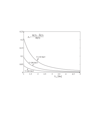
Figure 1: The relative difference $\Delta_{3}=1-\hat{H}(3)/H(3)$ plotted versus $L_{\perp}$ for several values of the ”temperature” $T$.

In Figure 1, the relative difference

$$\Delta_{3}\equiv\frac{H(3)-\hat{H}(3)}{H(3)}=1-\frac{\log\hat{C}(3)}{\log C(3)}$$ (36)

is plotted versus $L_{\perp}$ for various values of $T$. One sees that for $T\geq 150$ MeV (corresponding to the average transverse momentum larger than 300 MeV), and $L_{\perp}\geq 3$ fm (appropriate for heavy ion collisions) $\Delta_{3}$ is indeed very small. We thus conclude that the moments of Wigner function reproduce the Renyi entropies of a multiparticle system created in high-energy nuclear collisions with rather good accuracy.

One sees also from Fig. 1 that the corrections increase at smaller values of $L_{\perp}$. At $L_{\perp}\approx 1$ fm (appropriate for elementary collisions) they reach about 20% for $T=150$ MeV and fall quickly at larger $T$. Thus, although for hadron-hadron and lepton-hadron collisions our estimates of Renyi entropy clearly require a more precise determination of the size of the system, they seem nevertheless to be within reach of the present experiments.

These two simple examples give only a general idea how to control the corrections. Estimates of corrections in more complicated situations are of course posssible, e.g., by Monte Carlo simulations.

6 Discussion and conclusions

Several comments are in order.

(i) Although we have discussed the general case of arbitrary $l$, it should be realized that, in practice, one may at best hope for the determination of the lowest order Renyi entropies $l=2,3$, perhaps also $l=4$. This implies that an extrapolation to $l=1$, giving the Shannon entropy (3), may require an independent input to be reliable [15].

(ii) One sees from (26) that for $l=2$ $a_{1}=0$, i.e., $C(2)=\hat{C}(2)$. Thus the Renyi entropy $H(2)$ does not suffer from the corrections discussed in this paper.

(iii) As is seen from the discussion in section 4, the difference between Renyi entropies and moments of the Wigner function depends primarily on the size of the system in configuration space. Also accuracy of the measurements of the moments of Wigner function depends on this size [8], as disussed in Section 3. One concludes that information from the HBT measurements [17, 18] is important for a successful application of the method.

(iv) One should keep in mind that we are discussing here the phase-space distribution and the Wigner function averaged over time. If the freeze-out takes relatively long time, the effective size of the system may be much larger than naively expected. On one hand this would improve the accuracy of the method. On the other hand it makes the estimate of the volume much more difficult, as the standard interpretation of the HBT measurements may be not adequate [19].

(v) It should be emphasized that the estimate of entropy investigated in the present paper takes explicitely into account the correlations between the particles observed in the experiment. This may be contrasted with the estimate obtained in [20] where the entropy of the multiparticle system is estimated from the single-particle inclusive distribution, thus ignoring the correlations between particles (except those induced by quantum interference). It would be very interesting to compare the results obtained from these two methods. This may provide an insight into the role of multiparticle correlations in counting the number of effective degrees of freedom of a multiparticle system.

(vi) The entropies we discuss refer to the particles actually measured in experiment in question. Therefore the result does depend on the nature of the detector. E.g., the results change when entropy is determined from all produced particles instead of only from the charged ones. This should not be surprising: the effective number of degrees of freedom naturally depends on the number and nature of the particles considered. Actually, investigations of the dependence of entropy on the number of particles may provide some interesting hints on the structure of produced final states.

(vii) Through this paper we have only discussed entropies of the M-particle distribution at fixed $M$. One is often interested in entropies summed over all multiplicities. They may be obtained from coincidence probabilities referred to all multiplicities, constructed following the formula

$$C(l)=\sum_{M}[P(M)]^{l}C_{M}(l),$$ (37)

where $P(M)$ is the multiplicity distribution and where, for the sake of clarity, we have added a subspript $M$ to denote the coincidence probability at fixed $M$. One sees that for large $l$ only multiplicities close to the most probable one contribute to the sum.

In conclusion, we have analyzed the relation between the moments of Wigner function (6) (which can be measured by counting the number of identical events [8]) and the coincidence probabilities (2) (which define the Renyi entropies). It was shown that, for a large class of models, these moments are identical to the coincidence probabilities in the limit of an infinite volume of the system. The finite volume corrections were discussed. They were shown to fall as the inverse square of the linear size of the system at freeze-out and turn out to be negligible for systems encountered in relativistic heavy ion collisions.

Acknowledgements

Discussions with Robi Peschanski and Jacek Wosiek were very useful and are highly appreciated. This investigation was partly supported by the MEiN research grant 1 P03B 045 29 (2005-2008).

References

- [1] A.Bialas and W.Czyz, Phys. Rev. D61 (2000) 074021.
- [2] A.Renyi, Proc. 4-th Berkeley Symp. Math. Stat. Prob. 1960, Vol.1, Univ. of California Press, Berkeley-Los Ageles 1961, p.547.
- [3] C.Beck and F.Schloegl, Thermodynamics of chaotic systems, Cambridge U. Press, Cambridge (1993).
- [4] For a recent discussion see, e.g. B.Muller and K.Rajagopal, hep-ph/0502174 and references therein.
- [5] G.F.Bertsch, Phys. Rev. Letters 72 (1994) 2349; 77 (1996) 789 (E).
- [6] D.A.Brown, S.Y.Panitkin and G.F.Bertsch, Phys. Rev. C62 (2000) 014904.
- [7] For a discussion of the physical meaning of the Wigner function see, e.g., M.Hillery, R.F.O’Connell, M.O.Scully and E.P.Wigner, Phys.Rept. 106 (1984) 121 and references therein.
- [8] A.Bialas, W.Czyz and K.Zalewski, Acta Phys. Pol. B36 (2005) 3109; hep-ph/0506233, to be published in Phys. Lett. B.
- [9] A.Bialas and W.Czyz, Acta Phys. Pol. B31 (2000) 687.
- [10] A.Bialas and W.Czyz, Acta Phys. Pol. B31 (2000) 2803; B34 (2003) 3363.
- [11] S.K.Ma, Statistical Mechanics, World Scientific, Singapore 1985; S.K.Ma, J. Stat. Phys. 26 (1981) 221.
- [12] A.Bialas, W.Czyz and J.Wosiek, Acta Phys. Pol. B30 (1999) 107.
- [13] It is obviously valid for models which assume thermal equilibrium. It is also valid in the blast-wave models, provided . The Hubble-like expansion is obtained for . For a review of models see, e.g., U.A. Wiedemann and U. Heinz, Phys. Rep. 319(1999)145; U. Heinz and B. Jacak, Ann. Rev. Nucl.Part.Sci. 49(1999)529; R.M. Weiner, Phys. Rep. 327(2000)250; T.Csorgo, H.I.Phys. 15 (2002)1.
- [14] K.Fialkowski and R.Wit, Phys.Rev. D62 (2000) 114016; NA22 coll, M. Atayan et al., Acta Phys. Pol. B36 (2005) 2969.
- [15] K.Zyczkowski, Open Sys. and Information Dyn. 10 (2003) 297.
- [16] A.Bialas and K.Zalewski, hep-ph 0512248, to be published in Acta Phys. Pol. B.
- [17] D.A.Brown and P.Danielewicz, Phys. Lett. B398 (1997) 252; Phys. Rev D58 (1998) 094003; S.Y.Panitkin and D.A.Brown, Phys. Rev C61 (1999) 021901; G.Verde et al, Phys. Rev. C65 (2002) 054609; P.Danielewicz et al., Acta Phys. Hung. A19 (2004) nucl-th/0407022.
- [18] Yu.M.Sinyukov and S.V.Akkelin, Heavy Ion Phys. 9 (1999); S.V.Akkelin and Yu.M.Sinyukov, nucl-th/0310036.
- [19] See, e.g., A.Bialas and K.Zalewski, Phys. Rev. D72 (2005) 036009.
- [20] S.Pal and S.Pratt, Phys. Lett. B578 (2004) 310.