Chiral perturbation theory

Abstract

Chiral perturbation theory is the effective field theory of the strong interactions at low energies. We will give a short introduction to chiral perturbation theory for mesons and will discuss, as an example, the electromagnetic polarizabilities of the pion. These have recently been extracted from an experiment on radiative $\pi^{+}$ photoproduction from the proton ($\gamma p\to\gamma\pi^{+}n$) at the Mainz Microtron MAMI. Next we will turn to the one-baryon sector of chiral perturbation theory and will address the issue of a consistent power counting scheme. As examples of the heavy-baryon framework we will comment on the extraction of the axial radius from pion electroproduction and will discuss the generalized polarizabilities of the proton. Finally, we will discuss two recently proposed manifestly Lorentz-invariant renormalization schemes and illustrate their application in a calculation of the nucleon electromagnetic form factors.

1 Introduction

Chiral perturbation theory (ChPT) Weinberg:1978kz ; Gasser:1983yg ; Gasser:1984gg ; Gasser:1987rb is the effective field theory (EFT) Ecker:2005ny of the strong interactions at low energies. The central idea of the EFT approach was formulated by Weinberg as follows Weinberg:1978kz : “… if one writes down the most general possible Lagrangian, including all terms consistent with assumed symmetry principles, and then calculates matrix elements with this Lagrangian to any given order of perturbation theory, the result will simply be the most general possible S–matrix consistent with analyticity, perturbative unitarity, cluster decomposition and the assumed symmetry principles.” In the context of the strong interactions these ideas have first been applied to the interactions among the Goldstone bosons of spontaneous symmetry breaking in quantum chromodynamics (QCD). The effective theory is formulated in terms of the asymptotically observed states instead of the quark and gluon degrees of freedom of the underlying (fundamental) theory, namely QCD. The corresponding EFT—mesonic chiral perturbation theory—has been tested at the two-loop level (see, e.g., Scherer:2002tk ; Scherer:2005ri for a pedagogical introduction). A successful EFT program requires both the knowledge of the most general Lagrangian up to and including the given order one is interested in as well as an expansion scheme for observables. Due to the vanishing of the Goldstone boson masses in the chiral limit in combination with their vanishing interactions in the zero-energy limit, a derivative and quark-mass expansion is a natural scenario for the corresponding EFT. At present, in the mesonic sector the Lagrangian is known up to and including ${\cal O}(q^{6})$, where $q$ denotes a small quantity such as a four momentum or a pion mass. The combination of dimensional regularization with the modified minimal subtraction scheme of ChPT Gasser:1983yg leads to a straightforward correspondence between the loop expansion and the chiral expansion in terms of momenta and quark masses at a fixed ratio, and provides a consistent power counting for renormalized quantities.

In the extension to the one-nucleon sector Gasser:1987rb an additional scale, namely the nucleon mass, enters the description. In contrast to the Goldstone boson masses, the nucleon mass does not vanish in the chiral limit. As a result, the straightforward correspondence between the loop expansion and the chiral expansion of the mesonic sector, at first sight, seems to be lost: higher-loop diagrams can contribute to terms as low as ${\cal O}(q^{2})$ Gasser:1987rb . This problem has been eluded in the framework of the heavy-baryon formulation of ChPT Jenkins:1990jv ; Bernard:1992qa , resulting in a power counting analogous to the mesonic sector. The basic idea consists in expressing the relativistic nucleon field in terms of a velocity-dependent field, thus dividing nucleon momenta into a large piece close to on-shell kinematics and a soft residual contribution. Most of the calculations in the one-baryon sector have been performed in this framework (for an overview see, e.g., Bernard:1995dp ) which essentially corresponds to a simultaneous expansion of matrix elements in $1/m$ and $1/(4\pi F_{\pi})$. However, there is price one pays when giving up manifest Lorentz invariance of the Lagrangian. At higher orders in the chiral expansion, the expressions due to the $1/m$ corrections of the Lagrangian become increasingly complicated Ecker:1995rk ; Fettes:2000gb . Moreover, not all of the scattering amplitudes, evaluated perturbatively in the heavy-baryon framework, show the correct analytical behavior in the low-energy region Bernard:1996cc . In recent years, there has been a considerable effort in devising renormalization schemes leading to a simple and consistent power counting for the renormalized diagrams of a manifestly Lorentz-invariant approach Tang:1996ca ; Ellis:1997kc ; Becher:1999he ; Lutz:1999yr ; Gegelia:1999gf ; Gegelia:1999qt ; Lutz:2001yb ; Fuchs:2003qc .

In the following we will highlight a few topics in chiral perturbation theory which have been subject of experimental tests at the Mainz Microtron MAMI.

2 Chiral perturbation theory for mesons

2.1 The effective Lagrangian and Weinberg’s power counting scheme

The starting point of mesonic chiral perturbation theory is a chiral $\mbox{SU}(N_{l})_{L}\times\mbox{SU}(N_{l})_{R}\times\mbox{U}(1)_{V}$ symmetry of the QCD Lagrangian for $N_{l}$ massless (light) quarks:

$${\cal L}^{0}_{\rm QCD}=\sum_{l=1}^{N_{l}}(\bar{q}_{R,l}iD/\hskip 3.00003ptq_{R,l}+\bar{q}_{L,l}iD/\hskip 3.00003ptq_{L,l})-\frac{1}{4}{\cal G}_{\mu\nu,a}{\cal G}^{\mu\nu}_{a}.$$ (1)

In eq. (1), $q_{L,l}$ and $q_{R,l}$ denote the left- and right-handed components of the light quark fields. Here, we will be concerned with the cases $N_{l}=2$ and $N_{l}=3$ referring to massless $u$ and $d$ or $u$, $d$ and $s$ quarks, respectively. Furthermore, we will neglect the terms involving the heavy quark fields. The covariant derivative $D_{\mu}q_{L/R,l}$ contains the flavor-independent coupling to the eight gluon gauge potentials, and ${\cal G}_{\mu\nu,a}$ are the corresponding field strengths. The Lagrangian of eq. (1) is invariant under separate global $\mbox{SU}(N_{l})_{L/R}$ transformations of the left- and right-handed fields. In addition, it has an overall $\mbox{U}(1)_{V}$ symmetry. Several empirical facts give rise to the assumption that this chiral symmetry is spontaneously broken down to its vectorial subgroup $\mbox{SU}(N_{l})_{V}\times\mbox{U}(1)_{V}$. For example, the low-energy hadron spectrum seems to follow multiplicities of the irreducible representations of the group $\mbox{SU}(N_{l})$ (isospin SU(2) or flavor SU(3), respectively) rather than $\mbox{SU}(N_{l})_{L}\times\mbox{SU}(N_{l})_{R}$, as indicated by the absence of degenerate multiplets of opposite parity. Moreover, the lightest mesons form a pseudoscalar octet with masses that are considerably smaller than those of the corresponding vector mesons. According to Coleman’s theorem Coleman:1966 , the symmetry pattern of the spectrum reflects the invariance of the vacuum state. Therefore, as a result of Goldstone’s theorem Goldstone:1961eq ; Goldstone:1962es , one would expect $6-3=3$ or $16-8=8$ massless Goldstone bosons for $N_{l}=2$ and $N_{l}=3$, respectively. These Goldstone bosons have vanishing interactions as their energies tend to zero. Of course, in the real world, the pseudoscalar meson multiplet is not massless which is a result of the finite quark masses of the $u$, $d$ and $s$ quarks. This explicit symmetry breaking in terms of the quark masses is treated perturbatively.

The symmetries as well as the symmetry breaking pattern of QCD—once the quark masses are included—are mapped onto the most general (effective) Lagrangian for the interaction of the Goldstone bosons. The Lagrangian is organized in the number of the (covariant) derivatives and of the quark mass terms Weinberg:1978kz ; Gasser:1983yg ; Gasser:1984gg ; Issler:1990nj ; Akhoury:1990px ; Scherer:1994wi ; Fearing:1994ga ; Bijnens:1999sh ; Ebertshauser:2001nj ; Bijnens:2001bb

$${\cal L}_{\pi}={\cal L}_{2}+{\cal L}_{4}+{\cal L}_{6}+\cdots,$$ (2)

where the lowest-order Lagrangian is given by

$${\cal L}_{2}=\frac{F^{2}}{4}\mbox{Tr}\Big{[}D_{\mu}U(D^{\mu}U)^{\dagger}+\chi U^{\dagger}+U\chi^{\dagger}\Big{]}.$$ (3)

Here,

$$U(x)=\exp\left(i\frac{\phi}{F}\right),\quad\phi=\left(\begin{array}[]{cc}\pi^{0}&\sqrt{2}\pi^{+}\\ \sqrt{2}\pi^{-}&-\pi^{0}\end{array}\right),$$

is a unimodular unitary $(2\times 2)$ matrix containing the Goldstone boson fields. In eq. (3), $F$ denotes the pion-decay constant in the chiral limit: $F_{\pi}=F[1+{\cal O}(\hat{m})]=92.4$ MeV. When including the electromagnetic interaction, the covariant derivative is defined as $D_{\mu}U=\partial_{\mu}U+ieA_{\mu}[Q,U],$ where $Q=\mbox{diag}(2/3,-1/3)$ denotes the quark charge matrix. We work in the isospin-symmetric limit $m_{u}=m_{d}=\hat{m}$. The quark masses are contained in $\chi=2B\hat{m}=M^{2}$, where $M^{2}$ denotes the lowest-order expression for the squared pion mass and $B$ is related to the quark condensate $\langle\bar{q}q\rangle_{0}$ in the chiral limit. The next-to-leading-order Lagrangian contains 7 low-energy constants $l_{i}$ Gasser:1983yg

$${\cal L}_{4}=l_{5}\left[\mbox{Tr}(f^{R}_{\mu\nu}Uf_{L}^{\mu\nu}U^{\dagger})-\frac{1}{2}\mbox{Tr}(f_{\mu\nu}^{L}f_{L}^{\mu\nu}+f_{\mu\nu}^{R}f_{R}^{\mu\nu})\right]$$ (4)

$$+i\frac{l_{6}}{2}\mbox{Tr}\left(f^{R}_{\mu\nu}D^{\mu}U(D^{\nu}U)^{\dagger}+f^{L}_{\mu\nu}(D^{\mu}U)^{\dagger}D^{\nu}U\right)+\cdots,$$

where we have displayed those terms which will be relevant for the discussion of Compton scattering below. In that case, the field strength is given by

$$f^{R}_{\mu\nu}=f^{L}_{\mu\nu}=-e(\partial_{\mu}A_{\nu}-\partial_{\nu}A_{\mu})Q.$$

In addition to the most general Lagrangian, one needs a method to assess the importance of various diagrams calculated from the effective Lagrangian. Using Weinberg’s power counting scheme Weinberg:1978kz one may analyze the behavior of a given diagram calculated in the framework of eq. (2) under a linear re-scaling of all external momenta, $p_{i}\mapsto tp_{i}$, and a quadratic re-scaling of the light quark masses, $\hat{m}\mapsto t^{2}\hat{m}$, which, in terms of the Goldstone boson masses, corresponds to $M^{2}\mapsto t^{2}M^{2}$. The chiral dimension $D$ of a given diagram with amplitude ${\cal M}(p_{i},\hat{m})$ is defined by

$${\cal M}(tp_{i},t^{2}\hat{m})=t^{D}{\cal M}(p_{i},\hat{m}),$$ (5)

where, in $n$ dimensions,

$$D = nN_{L}-2I_{\pi}+\sum_{k=1}^{\infty}2kN_{2k}^{\pi}$$ (6)

$$= 2+(n-2)N_{L}+\sum_{k=1}^{\infty}2(k-1)N_{2k}^{\pi}$$

$$\geq \mbox{2 in 4 dimensions}.$$

Here, $N_{L}$ is the number of independent loop momenta, $I_{\pi}$ the number of internal pion lines, and $N_{2k}^{\pi}$ the number of vertices originating from ${\cal L}_{2k}$. A diagram with chiral dimension $D$ is said to be of order ${\cal O}(q^{D})$. Clearly, for small enough momenta and masses diagrams with small $D$, such as $D=2$ or $D=4$, should dominate. Of course, the re-scaling of eq. (5) must be viewed as a mathematical tool. While external three-momenta can, to a certain extent, be made arbitrarily small, the re-scaling of the quark masses is a theoretical instrument only. Note that, for $n=4$, loop diagrams are always suppressed due to the term $2N_{L}$ in eq. (2.1). In other words, we have a perturbative scheme in terms of external momenta and masses which are small compared to some scale (here $4\pi F\approx 1$ GeV).

Figure 1: One-loop contribution to the pion self-energy. The number 2 in the interaction blob refers to ${\cal L}_{2}$.

Figure 2: Four-loop contribution to the pion self-energy.

Figures 1 and 2 show contributions to the pion self-energy with $D=4\cdot 1-2\cdot 1+2\cdot 1=4$ and $D=4\cdot 4-2\cdot 5+2\cdot 2=10$, respectively. As a specific example, let us consider the contribution of fig. 1 to the pion self-energy. Without going into the details, the explicit result of the one-loop contribution is given by (see, e.g., Scherer:2002tk )

$$\Sigma_{\rm loop}(p^{2})=\frac{4p^{2}-M^{2}}{6F^{2}}I_{\pi}(M^{2},\mu^{2},n)={\cal O}(q^{4}),$$

where the dimensionally regularized integral is given by

$$I_{\pi}(M^{2},\mu^{2},n)=\frac{M^{2}}{16\pi^{2}}\left[R+\ln\left(\frac{M^{2}}{\mu^{2}}\right)\right]+O(n-4).$$ (8)

In eq. (8), $R$ is defined as

$$R=\frac{2}{n-4}-[\mbox{ln}(4\pi)-\gamma_{E}+1],$$ (9)

with $n$ denoting the number of space-time dimensions and $\gamma_{E}=-\Gamma^{\prime}(1)$ being Euler’s constant. Note that both factors—the fraction and the integral—each count as ${\cal O}(q^{2})$ resulting in ${\cal O}(q^{4})$ for the total expression as anticipated. In other words, when calculating one-loop graphs, using vertices from ${\cal L}_{2}$ of eq. (3), one generates infinities (so-called ultraviolet divergences). In the framework of dimensional regularization these divergences appear as poles at space-time dimension $n=4$, since $R$ is infinite as $n\to 4$. The loop diagrams are renormalized by absorbing the infinite parts into the redefinition of the fields and the parameters of the most general Lagrangian. Since ${\cal L}_{2}$ of eq. (3) is not renormalizable in the traditional sense, the infinities cannot be absorbed by a renormalization of the coefficients $F$ and $B$. However, to quote from ref. Weinberg:1995mt : “… the cancellation of ultraviolet divergences does not really depend on renormalizability; as long as we include every one of the infinite number of interactions allowed by symmetries, the so-called non-renormalizable theories are actually just as renormalizable as renormalizable theories.” According to Weinberg’s power counting of eq. (2.1), one-loop graphs with vertices from ${\cal L}_{2}$ are of ${\cal O}(q^{4})$. The conclusion is that one needs to adjust (renormalize) the parameters of ${\cal L}_{4}$ to cancel one-loop infinities. In doing so, one still has the freedom of choosing a suitable renormalization condition. For example, in the minimal subtraction scheme (MS) one would fix the parameters of the counterterm Lagrangian such that they would precisely absorb the contributions proportional to $2/(n-4)$ . In the modified minimal subtraction scheme of ChPT ($\widetilde{\rm MS}$) employed in Gasser:1983yg , the seven (bare) coefficients $l_{i}$ of the ${\cal O}(q^{4})$ Lagrangian of (4) are expressed in terms of renormalized coefficients $l_{i}^{r}$ as

$$l_{i}=l_{i}^{r}+\gamma_{i}\frac{R}{32\pi^{2}},$$ (10)

where the $\gamma_{i}$ are fixed numbers.

2.2 Electromagnetic polarizabilities of the pion

In the framework of classical electrodynamics, the electric and magnetic polarizabilities $\alpha$ and $\beta$ describe the response of a system to a static, uniform, external electric and magnetic field in terms of induced electric and magnetic dipole moments. In principle, empirical information on the pion polarizabilities can be obtained from the differential cross section of low-energy Compton scattering on a charged pion

$$\frac{d\sigma}{d\Omega_{lab}}=\left(\frac{\omega^{\prime}}{\omega}\right)^{2}\frac{e^{2}}{4\pi M_{\pi}}\left\{\frac{e^{2}}{4\pi M_{\pi}}\frac{1+z^{2}}{2}\right.$$

$$\left.-\frac{\omega\omega^{\prime}}{2}\left[(\alpha+\beta)_{\pi^{+}}(1+z)^{2}+(\alpha-\beta)_{\pi^{+}}(1-z)^{2}\right]\right\}$$

$$+\cdots,$$

where $z=\hat{q}\cdot\hat{q}\,^{\prime}$ and $\omega^{\prime}/\omega=[1+\omega(1-z)/M_{\pi}]$. The forward and backward differential cross sections are sensitive to $(\alpha+\beta)_{\pi^{+}}$ and $(\alpha-\beta)_{\pi^{+}}$, respectively.

The predictions for the charged pion polarizabilities at ${\cal O}(q^{4})$ Bijnens:1987dc result from an old current-algebra low-energy theorem Terentev:1972ix

$$\alpha_{\pi^{+}}=-\beta_{\pi^{+}} = 2\frac{e^{2}}{4\pi}\frac{1}{(4\pi F_{\pi})^{2}M_{\pi}}\frac{\bar{l}_{6}-\bar{l}_{5}}{6}$$

$$= (2.64\pm 0.09)\times 10^{-4}\,\mbox{fm}^{3},$$

which relates Compton scattering on a charged pion, $\gamma\pi^{+}\to\gamma\pi^{+}$, in terms of a chiral Ward identity to radiative charged-pion beta decay, $\pi^{+}\to e^{+}\nu_{e}\gamma$. The linear combination $\bar{l}_{6}-\bar{l}_{5}$ of scale-independent low-energy constants Gasser:1983yg is fixed using the most recent determination of the ratio of the pion axial-vector form factor $F_{A}$ and the vector form factor $F_{V}$ via the radiative pion beta decay Frlez:2003pe :

$$\gamma=\frac{1}{6}(\bar{l}_{6}-\bar{l}_{5})=\frac{F_{A}}{F_{V}}=0.443\pm 0.015.$$

A two-loop analysis (${\cal O}(q^{6})$) of the charged-pion polarizabilities has been worked out in Burgi:1996mm ; Burgi:1996qi :

$$(\alpha+\beta)_{\pi^{+}} = (0.3\pm 0.1)\times 10^{-4}\,\mbox{fm}^{3},$$ (11)

$$(\alpha-\beta)_{\pi^{+}} = (4.4\pm 1.0)\times 10^{-4}\,\mbox{fm}^{3}.$$ (12)

The degeneracy $\alpha_{\pi^{+}}=-\beta_{\pi^{+}}$ is lifted at the two-loop level. The corresponding corrections amount to an 11% (22%) change of the ${\cal O}(q^{4})$ result for $\alpha_{\pi^{+}}$ ($\beta_{\pi^{+}}$), indicating a similar rate of convergence as for the $\pi\pi$-scattering lengths Gasser:1983yg ; Bijnens:1995yn . The effect of the new low-energy constants appearing at ${\cal O}(q^{6})$ on the pion polarizability was estimated via resonance saturation by including vector and axial-vector mesons. The contribution was found to be about 50% of the two-loop result. However, one has to keep in mind that Burgi:1996mm ; Burgi:1996qi could not yet make use of the improved analysis of radiative pion decay which, in the meantime, has also been evaluated at two-loop accuracy Bijnens:1996wm ; Geng:2003mt . Taking higher orders in the quark mass expansion into account, Bijnens and Talavera obtain $(\bar{l}_{6}-\bar{l}_{5})=2.98\pm 0.33$ Bijnens:1996wm , which would slightly modify the leading-order prediction to $\alpha_{\pi^{+}}=(2.96\pm 0.33)\times 10^{-4}\,\mbox{fm}^{3}$ instead of $\alpha_{\pi^{+}}=(2.7\pm 0.4)\times 10^{-4}\,\mbox{fm}^{3}$ used in Burgi:1996mm ; Burgi:1996qi . Accordingly, the difference $(\alpha-\beta)_{\pi^{+}}$ of (12) would increase to $4.9\times 10^{-4}\,\mbox{fm}^{3}$ instead of $4.4\times 10^{-4}\,\mbox{fm}^{3}$, whereas the sum would remain the same as in eq. (11).

As there is no stable pion target, empirical information about the pion polarizabilities is not easy to obtain. For that purpose, one has to consider reactions which contain the Compton scattering amplitude as a building block, such as, e.g., the Primakoff effect in high-energy pion-nucleus bremsstrahlung, $\pi^{-}Z\to\pi^{-}Z\gamma$ Antipov:1982kz , radiative pion photoproduction on the nucleon, $\gamma p\to\gamma\pi^{+}n$ Aibergenov:1986gi ; Ahrens:2004mg , and pion pair production in $e^{+}e^{-}$ scattering, $e^{+}e^{-}\to e^{+}e^{-}\pi^{+}\pi^{-}$ Berger:1984xb ; Courau:1986gn ; Ajaltoni ; Boyer:1990vu . The results of the older experiments are summarized in table 1.

Table 1: Previous experimental data on the charged pion polarizability $\alpha_{\pi^{+}}$.

Reaction	Experiment	$\alpha_{\pi^{+}}$ [$10^{-4}$ $\mbox{fm}^{3}$]
$\pi^{-}Z\rightarrow\pi^{-}Z\gamma$	Serpukhov Antipov:1982kz	$6.8\pm 1.4\pm 1.2$
$\gamma p\to\gamma\pi^{+}n$	Lebedev Phys. Inst. Aibergenov:1986gi	$20\pm 12$
$\gamma\gamma\rightarrow\pi^{+}\pi^{-}$	PLUTO Berger:1984xb	$19.1\pm 4.8\pm 5.7$
	DM 1 Courau:1986gn	$17.2\pm 4.6$
	DM 2 Ajaltoni	$26.3\pm 7.4$
	MARK II Boyer:1990vu	$2.2\pm 1.6$

The potential of studying the influence of the pion polarizabilities on radiative pion photoproduction from the proton was extensively studied in Drechsel:1994kh . In terms of Feynman diagrams, the reaction $\gamma p\to\gamma\pi^{+}n$ contains real Compton scattering on a charged pion as a pion pole diagram (see fig. 3). In the recent experiment on $\gamma p\to\gamma\pi^{+}n$ at the Mainz Microtron MAMI Ahrens:2004mg , the cross section was obtained in the kinematic region 537 MeV $<E_{\gamma}<$ 817 MeV, $140^{\circ}\leq\theta^{\rm cm}_{\gamma\gamma^{\prime}}\leq 180^{\circ}$. The values of the pion polarizabilities have been obtained from a fit of the cross section calculated by different theoretical models to the data rather than performing an extrapolation to the $t$-channel pole of the Chew-Low type Chew:1958wd ; Unkmeir . Figure 4 shows the experimental data, averaged over the full photon beam energy interval and over the squared pion-photon center-of-mass energy $s_{1}$ from 1.5 $M_{\pi}^{2}$ to 5 $M_{\pi}^{2}$ as a function of the squared pion momentum transfer $t$ in units of $M_{\pi}^{2}$. For such small values of $s_{1}$, the differential cross section is expected to be insensitive to the pion polarizabilities. Also shown are two model calculations: model 1 (solid curve) is a simple Born approximation using the pseudoscalar pion-nucleon interaction including the anomalous magnetic moments of the nucleon; model 2 (dashed curve) consists of pole terms without the anomalous magnetic moments but including contributions from the resonances $\Delta(1232)$, $P_{11}(1440)$, $D_{13}(1520)$ and $S_{11}(1535)$. The dotted curve is a fit to the experimental data.

The kinematic region where the polarizability contribution is biggest is given by $5M_{\pi}^{2}<s_{1}<15M_{\pi}^{2}$ and $-12M_{\pi}^{2}<t<-2M_{\pi}^{2}$. Figure 5 shows the cross section as a function of the beam energy integrated over $s_{1}$ and $t$ in this second region. The dashed and solid lines (dashed-dotted and dotted lines) refer to models 1 and 2, respectively, each with $(\alpha-\beta)_{\pi^{+}}=0$ ($(\alpha-\beta)_{\pi^{+}}=14\times 10^{-4}\,\mbox{fm}^{3}$). By comparing the experimental data of the 12 points with the predictions of the models, the corresponding values of $(\alpha-\beta)_{\pi^{+}}$ for each data point have been determined in combination with the corresponding statistical and systematic errors. The result extracted from the combined analysis of the 12 data points reads Ahrens:2004mg

$$(\alpha-\beta)_{\pi^{+}}=(11.6\pm 1.5_{\rm stat}\pm 3.0_{\rm syst}\pm 0.5_{\rm mod})\times 10^{-4}\,\mbox{fm}^{3}$$ (13)

and has to be compared with the ChPT result of, say, $(4.9\pm 1.0)\times 10^{-4}\,\mbox{fm}^{3}$ which deviates by 2 standard deviations from the experimental result. On the other hand, the application of dispersion sum rules as performed in Fil'kov:1998np yields $(\alpha-\beta)_{\pi^{+}}=(10.3\pm 1.9)\times 10^{-4}\,\mbox{fm}^{3}$.

Both the precision measurement of radiative pion beta decay Frlez:2003pe and of radiative pion photoproduction indicate that further theoretical and experimental work is needed. In particular, the analysis of ref. Frlez:2003pe suggests an inadequacy of the present $V-A$ description of the radiative beta decay, which would also reflect itself in an inadequacy of the ChPT description in its present form. What remains to be understood is why the dispersion sum rules give such a dramatically different result from the ChPT calculation where the higher-order terms have been estimated from resonance saturation by including vector and axial-vector mesons. Clearly, the model-dependent input deserves further study. In this context, a full and consistent one-loop calculation of $\gamma p\to\gamma\pi^{+}n$ including the Delta resonance Hacker:2005fh would be desirable.

For a discussion of the so-called generalized pion polarizabilities see Unkmeir:1999md ; Fuchs:2000pn ; L'vov:2001fz ; Unkmeir:2001gw .

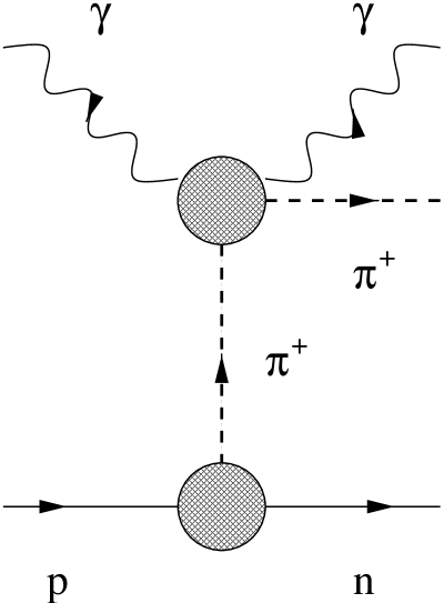
Figure 3: The reaction $\gamma p\to\gamma\pi^{+}n$ contains Compton scattering on a pion as a sub diagram in the $t$ channel, where $t=(p_{n}-p_{p})^{2}$.

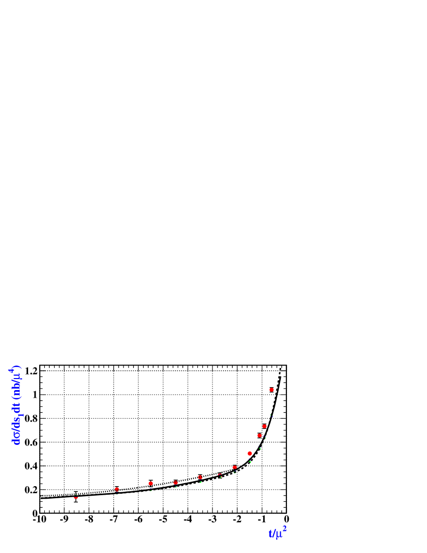
Figure 4: Differential cross section averaged over 537 MeV $<E_{\gamma}<$ 817 MeV and 1.5 $M_{\pi}^{2}<s_{1}<5M_{\pi}^{2}$. Solid line: model 1; dashed line: model 2; dotted line: fit to experimental data.

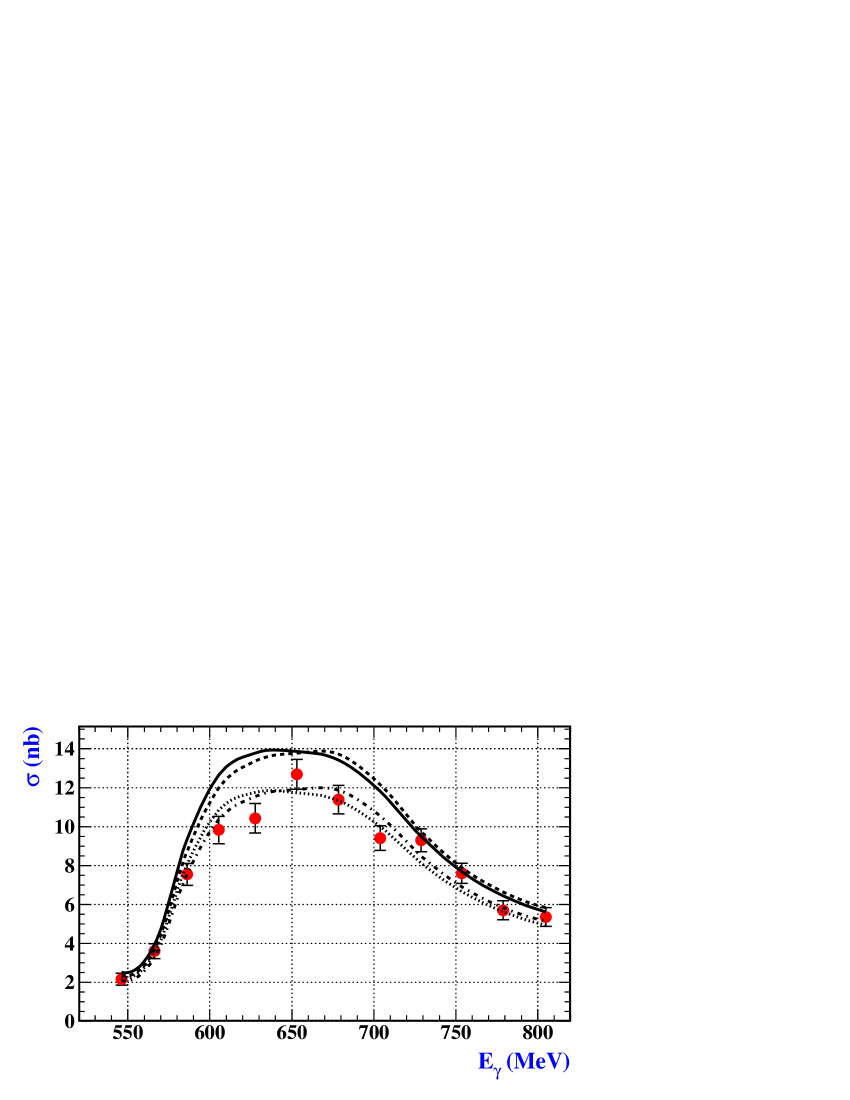
Figure 5: The cross section of the process $\gamma p\to\gamma\pi^{+}n$ integrated over $s_{1}$ and $t$ in the region where the contribution of the pion polarizability is biggest and the difference between the predictions of the theoretical models under consideration does not exceed 3 %. The dashed and dashed-dotted lines are predictions of model 1 and the solid and dotted lines of model 2 for $(\alpha-\beta)_{\pi^{+}}=0$ and $(\alpha-\beta)_{\pi^{+}}=14\times 10^{-4}\,\mbox{fm}^{3}$, respectively.

2.3 Future perspectives at MAMI

With the setup of the Crystal Ball detector, a dedicated $\eta$ physics program will be possible at MAMI. In the reaction $\gamma+p\to p+\eta$, $10^{7}$ etas will be produced per day. The main physics objectives will be the investigation of neutral decay channels.

In the framework of $\mbox{SU(3)}_{L}\times\mbox{SU(3)}_{R}$ symmetry the decay process $\eta\to\pi^{0}\gamma\gamma$ is closely related to $\gamma\gamma\to\pi^{0}\pi^{0}$. At ${\cal O}(q^{4})$, the amplitude is given entirely in terms of one-loop diagrams involving vertices of ${\cal O}(q^{2})$. The prediction for the decay width was found to be two orders of magnitude smaller Ametller:1991dp than the measured value. The pion loops are small due to approximate $G$-parity invariance whereas the kaon loops are suppressed by the large kaon mass in the propagator. Therefore, higher-order contributions must play a dominant role in $\eta\to\pi^{0}\gamma\gamma$. Even at ${\cal O}(q^{6})$ differences of a factor of two are found for the decay rate and spectrum Ametller:1991dp ; Ko:1993rg ; Bellucci:1995ay ; Bel'kov:1995fj ; Jetter:1995js ; Bijnens:1995vg ; Oset:2002sh although the most recent result for the decay width of $\Gamma(\eta\to\pi^{0}\gamma\gamma)=(0.45\pm 0.12)$ eV agrees with the original prediction $(0.42\pm 0.20)$ eV of ref. Ametller:1991dp . The decay $\eta\to\pi^{0}\pi^{0}\pi^{0}$ is a sensitive test of isospin symmetry violation with the transition amplitude being proportional to the light quark mass difference $(m_{u}-m_{d})$ Gasser:1984pr ; Leutwyler:1996tz . Moreover, the electromagnetic interaction was shown to produce only a small contribution Baur:1995gc . As a final example for “allowed” decays we refer to the rare eta decay $\eta\to\pi^{0}\pi^{0}\gamma\gamma$ Knochlein:1996ah ; Nefkens:2005ka . On the other hand, in the forbidden decays such as $\eta\to\pi^{0}\pi^{0}$ and $\eta\to 4\pi^{0}$ one will investigate (P,CP) violation which may be connected to the so-called $\theta$ term in QCD.

As a final example we would like to point at the potential of investigating the $\gamma\pi^{+}\to\pi^{+}\pi^{0}$ amplitude in the $\gamma p\to n\pi^{+}\pi^{0}$ reaction. This would allow for an alternative test of the Wess Zumino Witten action Wess:1971yu ; Witten:1983tw in terms of the ${\cal F}_{3\pi}$ amplitude (see Giller:2005uy for a recent overview).

3 Chiral perturbation theory for baryons

3.1 The power counting problem

The standard effective Lagrangian relevant to the single-nucleon sector contains, in addition to eq. (2), the most general $\pi N$ Lagrangian Gasser:1987rb ; Ecker:1995rk ; Fettes:2000gb ,

$${\cal L}_{\pi N}={\cal L}_{\pi N}^{(1)}+{\cal L}_{\pi N}^{(2)}+\cdots.$$ (14)

Due to the additional spin degree of freedom ${\cal L}_{\pi N}$ contains both odd and even powers in small quantities. In order to illustrate the issue of power counting in the baryonic sector, we consider the lowest-order $\pi N$ Lagrangian Gasser:1987rb , expressed in terms of bare fields and parameters denoted by subscripts 0,

$${\cal L}_{\pi N}^{(1)}=\bar{\Psi}_{0}\left(i\gamma_{\mu}\partial^{\mu}-m_{0}-\frac{1}{2}\frac{{\stackrel{{\scriptstyle\circ}}{{g_{A}}}}_{0}}{F_{0}}\gamma_{\mu}\gamma_{5}\tau^{a}\partial^{\mu}\pi^{a}_{0}\right)\Psi_{0}+\cdots,$$ (15)

where $\Psi_{0}$ and $\vec{\pi}_{0}$ denote a doublet and a triplet of bare nucleon and pion fields, respectively. After renormalization, $m$, $\stackrel{{\scriptstyle\circ}}{{g_{A}}}$, and $F$ refer to the chiral limit of the physical nucleon mass, the axial-vector coupling constant, and the pion-decay constant, respectively.

In sec. 2.1 we saw that, in the purely mesonic sector, contributions of $n$-loop diagrams are at least of order ${\cal O}(q^{2n+2})$, i.e., they are suppressed by $q^{2n}$ in comparison with tree-level diagrams. An important ingredient in deriving this result was the fact that we treated the squared pion mass as a small quantity of order $q^{2}$. Such an approach is motivated by the observation that the masses of the Goldstone bosons must vanish in the chiral limit. In the framework of ordinary chiral perturbation theory $M_{\pi}^{2}\sim\hat{m}$ which translates into a momentum expansion of observables at fixed ratio $\hat{m}/p^{2}$. On the other hand, there is no reason to believe that the masses of hadrons other than the Goldstone bosons should vanish or become small in the chiral limit. In other words, the nucleon mass entering the pion-nucleon Lagrangian of eq. (15) should not be treated as a small quantity of, say, order ${\cal O}(q)$. Naturally the question arises how all this affects the calculation of loop diagrams and the setup of a consistent power counting scheme.

Our goal is to propose a renormalization procedure generating a power counting for tree-level and loop diagrams of the (relativistic) EFT for baryons which is analogous to that given in sec. 2.1 for mesons. Choosing a suitable renormalization condition will allow us to apply the following power counting: a loop integration in $n$ dimensions counts as $q^{n}$, pion and fermion propagators count as $q^{-2}$ and $q^{-1}$, respectively, vertices derived from ${\cal L}_{2k}$ and ${\cal L}_{\pi N}^{(k)}$ count as $q^{2k}$ and $q^{k}$, respectively. Here, $q$ generically denotes a small expansion parameter such as, e.g., the pion mass. In total this yields for the power $D$ of a diagram in the one-nucleon sector the standard formula

$$D = nN_{L}-2I_{\pi}-I_{N}+\sum_{k=1}^{\infty}2kN^{\pi}_{2k}+\sum_{k=1}^{\infty}kN_{k}^{N}$$

$$= 1+(n-2)N_{L}+\sum_{k=1}^{\infty}2(k-1)N^{\pi}_{2k}+\sum_{k=1}^{\infty}(k-1)N_{k}^{N}$$

$$\geq \mbox{1 in 4 dimensions},$$

where $N_{L}$, $I_{\pi}$, $I_{N}$, $N_{2k}^{\pi}$, and $N_{k}^{N}$ denote the number of independent loop momenta, internal pion lines, internal nucleon lines, vertices originating from ${\cal L}_{2k}$, and vertices originating from ${\cal L}_{\pi N}^{(k)}$, respectively.

According to eq. (3.1), one-loop calculations in the single-nucleon sector should start contributing at ${\cal O}(q^{n-1})$. For example, let us consider the one-loop contribution of fig. 6 to the nucleon self-energy. According to eq. (3.1), the renormalized result should be of the order

$$D=n\cdot 1-2\cdot 1-1\cdot 1+1\cdot 2=n-1.$$ (18)

We will see below that the corresponding renormalization scheme is more complicated than in the mesonic sector.

Figure 6: One-loop contribution to the nucleon self-energy. The number 1 in the interaction blobs refers to ${\cal L}_{\pi N}^{(1)}$.

An explicit calculation yields Fuchs:2003qc

$$\Sigma_{\rm loop}=-\frac{3{\stackrel{{\scriptstyle\circ}}{{g_{A}}}}_{0}^{2}}{4F_{0}^{2}}\left\{\vphantom{-\frac{(p^{2}-m^{2})p/}{2p^{2}}}(p/\hskip 1.00006pt+m)I_{N}+M^{2}(p/\hskip 1.00006pt+m)I_{N\pi}(-p,0)\right.$$

$$\left.-\frac{(p^{2}-m^{2})p/\hskip 1.00006pt}{2p^{2}}[(p^{2}-m^{2}+M^{2})I_{N\pi}(-p,0)+I_{N}-I_{\pi}]\right\},$$

where the relevant loop integrals are defined as

$$I_{\pi} = \mu^{4-n}\int\frac{d^{n}k}{(2\pi)^{n}}\frac{i}{k^{2}-M^{2}+i0^{+}},$$ (19)

$$I_{N} = \mu^{4-n}\int\frac{d^{n}k}{(2\pi)^{n}}\frac{i}{k^{2}-m^{2}+i0^{+}},$$ (20)

$$I_{N\pi}(-p,0) = \mu^{4-n}\int\frac{d^{n}k}{(2\pi)^{n}}\frac{i}{[(k-p)^{2}-m^{2}+i0^{+}]}$$ (21)

$$\hskip 20.00003pt\times\frac{1}{k^{2}-M^{2}+i0^{+}}.$$

Applying the $\widetilde{\rm MS}$ renormalization scheme of ChPT Gasser:1983yg ; Gasser:1987rb —indicated by “r”—one obtains

$$\Sigma_{\rm loop}^{r}=-\frac{3g_{Ar}^{2}}{4F_{r}^{2}}\left[-\frac{M^{2}}{16\pi^{2}}(p/\hskip 1.00006pt+m)+\cdots\right]={\cal O}(q^{2}),$$

where $M^{2}$ is the lowest-order expression for the squared pion mass. In other words, the $\widetilde{\rm MS}$-renormalized result does not produce the desired low-energy behavior of eq. (18). This finding has widely been interpreted as the absence of a systematic power counting in the relativistic formulation of ChPT.

3.2 Heavy-baryon approach

One possibility of overcoming the problem of power counting was provided in terms of heavy-baryon chiral perturbation theory (HBChPT) Jenkins:1990jv ; Bernard:1992qa resulting in a power counting scheme which follows eqs. (3.1) and (3.1). The basic idea consists in dividing nucleon momenta into a large piece close to on-shell kinematics and a soft residual contribution: $p=mv+k_{p}$, $v^{2}=1$, $v^{0}\geq 1$ [often $v^{\mu}=(1,0,0,0)$]. The relativistic nucleon field is expressed in terms of velocity-dependent fields,

$$\Psi(x)=e^{-imv\cdot x}({\cal N}_{v}+{\cal H}_{v}),$$

with

$${\cal N}_{v}=e^{+imv\cdot x}\frac{1}{2}(1+v/)\Psi,\quad{\cal H}_{v}=e^{+imv\cdot x}\frac{1}{2}(1-v/)\Psi.$$

Using the equation of motion for ${\cal H}_{v}$, one can eliminate ${\cal H}_{v}$ and obtain a Lagrangian for ${\cal N}_{v}$ which, to lowest order, reads Bernard:1992qa

$$\widehat{\cal L}^{(1)}_{\pi N}=\bar{\cal N}_{v}(iv\cdot D+g_{A}S_{v}\cdot u){\cal N}_{v}+{\cal O}(1/m).$$

The result of the heavy-baryon reduction is a $1/m$ expansion of the Lagrangian similar to a Foldy-Wouthuysen expansion with a power counting along eqs. (3.1) and (3.1).

3.3 Pion electroproduction near threshold and the axial radius

As an example illustrating the strength of the EFT approach we consider pion electroproduction $\gamma^{\ast}(k)+N(p_{i})\to\pi^{i}(q)+N(p_{f})$ near threshold (for an overview, see ref. Drechsel:1992pn ) and the extraction of the nucleon axial radius. To that end we introduce the Green functions

$${\cal M}^{\mu}_{A,i} = \langle N(p_{f})|A^{\mu}_{i}(0)|N(p_{i})\rangle,$$

$${\cal M}_{JA,i}^{\mu\nu} = \int d\,^{4}x\,e^{iq\cdot x}\langle N(p_{f})|T\left[J^{\mu}(0)A^{\nu}_{i}(x)\right]|N(p_{i})\rangle,$$

$${\cal M}_{JP,i}^{\mu} = \int d\,^{4}x\,\,e^{iq\cdot x}\langle N(p_{f})|T\left[J^{\mu}(0)P_{i}(x)\right]|N(p_{i})\rangle,$$

where the subscripts $A$, $J$ and $P$ refer to axial-vector current, electromagnetic current and pseudoscalar density and $i$ refers to the $i$th isospin component of the axial-vector current or the pseudoscalar density, respectively. The so-called Adler-Gilman relation Adler:1966 provides the chiral Ward identity

$$q_{\nu}{\cal M}_{JA,i}^{\mu\nu}=i\hat{m}{\cal M}_{JP,i}^{\mu}+\epsilon_{3ij}{\cal M}^{\mu}_{A,j}$$ (22)

relating the three Green functions. In the one-photon-exchange approximation, the invariant amplitude for pion electroproduction can be written as ${\cal M}_{i}=-ie\epsilon_{\mu}{\cal M}^{\mu}_{i}$, where $\epsilon_{\mu}=e\bar{u}\gamma_{\mu}u/k^{2}$ is the polarization vector of the virtual photon and ${\cal M}^{\mu}_{i}$ the transition-current matrix element:

$${\cal M}^{\mu}_{i}=\langle N(p_{f}),\pi^{i}(q)|J^{\mu}(0)|N(p_{i})\rangle.$$ (23)

The relation between the Adler-Gilman relation, eq. (22), and pion electroproduction is established in terms of the Lehmann-Symanzik-Zimmermann reduction formula,

$${\cal M}^{\mu}_{i} = -i\frac{\hat{m}}{M_{\pi}^{2}F_{\pi}}\lim_{q^{2}\to M_{\pi}^{2}}(q^{2}-M_{\pi}^{2}){\cal M}_{JP,i}^{\mu}$$

$$= \frac{1}{M_{\pi}^{2}F_{\pi}}\lim_{q^{2}\to M_{\pi}^{2}}(q^{2}-M_{\pi}^{2})(\epsilon_{3ij}{\cal M}^{\mu}_{A,j}-q_{\nu}{\cal M}^{\mu\nu}_{JA,i}).$$

At threshold, the center-of-mass transition current can be parameterized in terms of two s-wave amplitudes $E_{0+}$ and $L_{0+}$

$$\left.e\vec{M}\right|_{\rm thr}=\frac{4\pi W}{m_{N}}\left[i\vec{\sigma}_{\perp}E_{0+}(k^{2})+i\vec{\sigma}_{\parallel}L_{0+}(k^{2})\right],$$

where $W$ is the total center-of-mass energy, $\vec{\sigma}_{\parallel}=\vec{\sigma}\cdot\hat{k}\hat{k}$ and $\vec{\sigma}_{\perp}=\vec{\sigma}-\vec{\sigma}_{\parallel}$.

Figure 7: One-loop contributions leading to a modification of the $k^{2}$ dependence of $E_{0+}^{(-)}$.

The contribution from pion loops (see fig. 7) has been analyzed in Bernard:1992ys and leads to a modification of the $k^{2}$ dependence of the electric dipole amplitude $E_{0+}^{(-)}$ [at ${\cal O}(q^{3})$]

$$E^{(-)}_{0+}(k^{2}) = \frac{eg_{A}}{8\pi F_{\pi}}\left[1+\frac{k^{2}}{4m^{2}_{N}}\left(\kappa_{v}+\frac{1}{2}\right)+\frac{k^{2}}{6}r^{2}_{A}\right.$$ (24)

$$+\left.\frac{M_{\pi}^{2}}{8\pi^{2}F^{2}_{\pi}}f\left(\frac{k^{2}}{M_{\pi}^{2}}\right)+\cdots\right],$$

where $\kappa_{v}=3.706$ is the isovector anomalous magnetic moment of the nucleon and $r_{A}$ is the axial radius. The first line corresponds to the traditional expression obtained in the framework of the partially conserved axial-vector current hypothesis (see, e.g., Scherer:1991cy ). The second line generates the modification

$$\frac{M_{\pi}^{2}}{8\pi^{2}F^{2}_{\pi}}f\left(\frac{k^{2}}{M_{\pi}^{2}}\right)=\frac{k^{2}}{128F^{2}_{\pi}}\left(1-\frac{12}{\pi^{2}}\right)+\cdots.$$

The reaction $p(e,e^{\prime}\pi^{+})n$ has been measured at MAMI at an invariant mass of $W=1125$ MeV (corresponding to a pion center of mass momentum of $|\vec{q}^{\ast}|=112$ MeV) and photon four-momentum transfers of $Q^{2}=0.117,0.195$ and 0.273 GeV² Liesenfeld:1999mv . Using an effective-Lagrangian model and a dipole form as an ansatz for the axial form factor $G_{A}$, an axial mass of

$$\tilde{M}_{A}=(1.077\pm 0.039)\,\mbox{GeV}$$

was extracted which has to be compared with the average of neutrino scattering experiments

$$M_{A}=(1.026\pm 0.021)\,\mbox{GeV}.$$

Defining $\tilde{M}_{A}=M_{A}+\Delta M_{A}$, the difference between the two results can nicely be explained in terms of the additional $k^{2}$ dependence of eq. (24) yielding $\Delta M_{A}=0.056$ GeV. In the meantime, the experiment has been repeated including an additional value of $Q^{2}=0.058$ GeV² Baumann:2004 and is currently being analyzed.

Recently, there have been claims that pion electroproduction data at threshold cannot be interpreted in terms of $G_{A}$ Haberzettl:2000sm . However, as was shown in Fuchs:2003vw , using minimal coupling alone does not respect the constraints due to chiral symmetry. In the framework of the most general Lagrangian, this can be seen by considering the $b_{23}$ term of the ${\cal O}(q^{3})$ Lagrangian Ecker:1995rk ,

$${\cal L}_{\rm eff}^{(3)}=\frac{1}{2(4\pi F)^{2}}b_{23}\,\bar{\Psi}\gamma^{\mu}\gamma_{5}[D^{\nu},f_{-\mu\nu}]\Psi+\cdots$$ (25)

with

$$f_{-\mu\nu} = -2(\partial_{\mu}a_{\nu}-\partial_{\nu}a_{\mu})+2i\left([v_{\mu},a_{\nu}]-[v_{\nu},a_{\mu}]\right)$$

$$+\frac{i}{F}\left[\vec{\tau}\cdot\vec{\pi},\partial_{\mu}v_{\nu}-\partial_{\nu}v_{\mu}\right]+\cdots.$$

The Lagrangian of eq. (25) is of a non-minimal type and the three terms contribute to the axial-vector matrix element, the $JA$ Green function and pion electroproduction relevant to the Adler-Gilman relation. As a result it was confirmed that threshold pion electroproduction is indeed a tool to obtain information on the axial form factor of the nucleon (see Fuchs:2003vw for details).

3.4 Virtual Compton scattering and generalized polarizabilities

As a second example, let us discuss the application of HBChPT to the calculation of the so-called generalized polarizabilities Arenhovel:1974 ; Guichon:1995pu . The virtual Compton scattering (VCS) amplitude $T_{\rm VCS}$ is accessible in the reaction $e^{-}p\to e^{-}p\gamma$. Model-independent predictions, based on Lorentz invariance, gauge invariance, crossing symmetry, and the discrete symmetries, have been derived in ref. Scherer:1996ux . Up to and including terms of second order in the momenta $|\vec{q}\,|$ and $|\vec{q}\,^{\prime}|$ of the virtual initial and real final photons, the amplitude is completely specified in terms of quantities which can be obtained from elastic electron-proton scattering and real Compton scattering, namely $m_{N}$, $\kappa$, $G_{E}$, $G_{M}$, $r^{2}_{E}$, $\alpha_{p}$ and $\beta_{p}$. The generalized polarizabilities (GPs) of ref. Guichon:1995pu result from an analysis of the residual piece in terms of electromagnetic multipoles. A restriction to the lowest-order, i.e. linear terms in $\omega^{\prime}$ leads to only electric and magnetic dipole radiation in the final state. Parity and angular-momentum selection rules, charge-conjugation symmetry, and particle crossing generate six independent GPs Guichon:1995pu ; Drechsel:1996ag ; Drechsel:1997xv .

The first results for the two structure functions $P_{LL}-P_{TT}/\epsilon$ and $P_{LT}$ at $Q^{2}=0.33$ GeV² were obtained from a dedicated VCS experiment at MAMI Roche:2000ng . Results at higher four-momentum transfer squared $Q^{2}=0.92$ and $Q^{2}=1.76$ GeV² have been reported in ref. Laveissiere:2004nf . Additional data are expected from MIT/Bates for $Q^{2}=0.05$ GeV² aiming at an extraction of the magnetic polarizability. Moreover, data in the resonance region have been taken at JLab for $Q^{2}=1$ GeV² Fonvieille:2004rb which have been analyzed in the framework of the dispersion relation formalism of ref. Pasquini:2001yy ; Drechsel:2002ar . Table 2 shows the experimental results of Roche:2000ng in combination with various model calculations. Clearly, the experimental precision of Roche:2000ng already allows for a critical test of the different models. Within ChPT and the linear sigma model, the GPs are essentially due to pionic degrees of freedom. Due to the small pion mass the effect in the spatial distributions extends to larger distances (see also fig. 9). On the other hand, the constituent quark model and other phenomenological models involving Gauß or dipole form factors typically show a faster decrease in the range $Q^{2}<1$ GeV².

Table 2: Experimental results and theoretical predictions for the structure functions $P_{LL}-P_{TT}/\epsilon$ and $P_{LT}$ at $Q^{2}=0.33$ GeV² and $\epsilon=0.62$. $\ast$ makes use of symmetry under particle crossing and charge conjugation which is not a symmetry of the nonrelativistic quark model.

	$P_{LL}-P_{TT}/\epsilon$ $[\mbox{GeV}^{-2}]$	$P_{LT}$ $[\mbox{GeV}^{-2}]$
Experiment Roche:2000ng	$23.7\pm 2.2_{\rm stat.}\pm 4.3_{\rm syst.}\pm 0.6_{\rm syst.norm.}$	$-5.0\pm 0.8_{\rm stat.}\pm 1.4_{\rm syst.}\pm 1.1_{\rm syst.norm.}$
Linear sigma model Metz:1996fn	11.5	0.0
Effective Lagrangian model Vanderhaeghen:1996iz	5.9	$-1.9$
HBChPT Hemmert:1997at	26.0	$-5.3$
Nonrelativistic quark model Pasquini:2000ue	$19.2|14.9^{\ast}$	$-3.2|-4.5^{\ast}$

A covariant definition of the spin-averaged dipole polarizabilities has been proposed in ref. L'vov:2001fz . It was shown that three generalized dipole polarizabilities are needed to reconstruct spatial distributions. For example, if the nucleon is exposed to a static and uniform external electric field $\vec{E}$, an electric polarization $\vec{\cal P}$ is generated which is related to the density of the induced electric dipole moments,

$${\cal P}_{i}(\vec{r})=4\pi\alpha_{ij}(\vec{r})\,E_{j}.$$ (26)

The tensor $\alpha_{ij}(\vec{r})$, i.e. the density of the full electric polarizability of the system, can be expressed as L'vov:2001fz

$$\alpha_{ij}(\vec{r}) = \alpha_{L}(r)\hat{r}_{i}\hat{r}_{j}+\alpha_{T}(r)(\delta_{ij}-\hat{r}_{i}\hat{r}_{j})$$

$$+\frac{3\hat{r}_{i}\hat{r}_{j}-\delta_{ij}}{r^{3}}\int_{r}^{\infty}[\alpha_{L}(r^{\prime})-\alpha_{T}(r^{\prime})]\,r^{\prime 2}\,dr^{\prime},$$

where $\alpha_{L}(r)$ and $\alpha_{T}(r)$ are Fourier transforms of the generalized longitudinal and transverse electric polarizabilities $\alpha_{L}(q)$ and $\alpha_{T}(q)$, respectively. In particular, it is important to realize that both longitudinal and transverse polarizabilities are needed to fully recover the electric polarization $\vec{\cal P}$. Figure 8 shows the induced polarization inside a proton as calculated in the framework of HBChPT at ${\cal O}(q^{3})$ Lvov:2004 and clearly shows that the polarization, in general, does not point into the direction of the applied electric field.

Similar considerations apply to an external magnetic field. Since the magnetic induction is always transverse (i.e., $\vec{\nabla}\cdot\vec{B}=0$), it is sufficient to consider $\beta_{ij}(\vec{r})=\beta(r)\delta_{ij}$ L'vov:2001fz . The induced magnetization $\vec{\cal M}$ is given in terms of the density of the magnetic polarizability as $\vec{\cal M}(\vec{r})=4\pi\beta(r)\vec{B}$ (see fig. 9).

Figure 8: Scaled electric polarization $r^{3}\alpha_{i1}$ [10^-3 fm³] Lvov:2004 . The applied electric field points in the $x$ direction.

Figure 9: Generalized magnetic polarizability $\beta(q^{2})$ and density of magnetic polarizability $\beta(r)$ for the proton. Dashed lines: contribution of pion loops; solid lines: total contribution; dotted lines: VMD predictions normalized to ${\beta}(0)$ L'vov:2001fz .

3.5 Manifestly Lorentz-invariant baryon chiral perturbation theory

Unfortunately, when considering higher orders in the chiral expansion, the expressions due to $1/m$ corrections of the Lagrangian become increasingly complicated. Secondly, not all of the scattering amplitudes, evaluated perturbatively in the heavy-baryon framework, show the correct analytical behavior in the low-energy region. Finally, with an increasing complexity of processes, the use of computer algebra systems becomes almost mandatory. The relevant techniques have been developed for calculations in the Standard Model and thus refer to loop integrals of the manifestly Lorentz-invariant type.

In the following we will concentrate on one of several methods that have been suggested to obtain a consistent power counting in a manifestly Lorentz-invariant approach Tang:1996ca ; Ellis:1997kc ; Becher:1999he ; Lutz:1999yr ; Gegelia:1999gf ; Gegelia:1999qt ; Lutz:2001yb ; Fuchs:2003qc , namely, the so-called extended on-mass-shell (EOMS) renormalization scheme Fuchs:2003qc . The central idea of the EOMS scheme consists of performing additional subtractions beyond the $\widetilde{\rm MS}$ scheme. Since the terms violating the power counting are analytic in small quantities, they can be absorbed by counterterm contributions. Let us illustrate the approach in terms of the integral

$$H(p^{2},m^{2};n)=\int\frac{d^{n}k}{(2\pi)^{n}}\frac{i}{[(k-p)^{2}-m^{2}+i0^{+}][k^{2}+i0^{+}]},$$

where $\Delta=(p^{2}-m^{2})/m^{2}={\cal O}(q)$ is a small quantity. We want the (renormalized) integral to be of the order $D=n-1-2=n-3$. Applying the dimensional counting analysis of ref. Gegelia:1994zz (for an illustration, see the appendix of ref. Schindler:2003je ), the result of the integration is of the form Fuchs:2003qc

$$H\sim F(n,\Delta)+\Delta^{n-3}G(n,\Delta),$$

where $F$ and $G$ are hypergeometric functions and are analytic in $\Delta$ for any $n$. Hence, the part containing $G$ for noninteger $n$ is proportional to a noninteger power of $\Delta$ and satisfies the power counting. On the other hand $F$ violates the power counting. The crucial observation is that the part proportional to $F$ can be obtained by first expanding the integrand in small quantities and then performing the integration for each term Gegelia:1994zz . This observation suggests the following procedure: expand the integrand in small quantities and subtract those (integrated) terms whose order is smaller than suggested by the power counting. In the present case, the subtraction term reads

$$H^{\rm subtr}=\int\frac{d^{n}k}{(2\pi)^{n}}\left.\frac{i}{[k^{2}-2p\cdot k+i0^{+}][k^{2}+i0^{+}]}\right|_{p^{2}=m^{2}}$$

and the renormalized integral is written as $H^{R}=H-H^{\rm subtr}={\cal O}(q)$ as $n\to 4$. In the infrared renormalization (IR) scheme of Becher and Leutwyler Becher:1999he , one would keep the contribution proportional to $G$ (with subtracted divergences when $n$ approaches 4) and completely drop the $F$ term.

Let us conclude this section with a few remarks. With a suitable renormalization condition one can also obtain a consistent power counting in manifestly Lorentz-invariant baryon chiral perturbation theory including, e.g., vector mesons Fuchs:2003sh or the $\Delta(1232)$ resonance Hacker:2005fh as explicit degrees of freedom. Secondly, the infrared regularization of Becher and Leutwyler Becher:1999he may be formulated in a form analogous to the EOMS renormalization Schindler:2003xv . Finally, using a toy model we have explicitly demonstrated the application of both infrared and extended on-mass-shell renormalization schemes to multiloop diagrams by considering as an example a two-loop self-energy diagram Schindler:2003je . In both cases the renormalized diagrams satisfy a straightforward power counting.

3.6 Applications

Figure 10: The Sachs form factors of the nucleon in manifestly Lorentz-invariant chiral perturbation theory at ${\cal O}(q^{4})$ without vector mesons. Full lines: results in the extended on-mass-shell scheme; dashed lines: results in infrared regularization. The experimental data are taken from ref. Friedrich:2003iz .

The EOMS scheme has been applied in several calculations such as the chiral expansion of the nucleon mass, the pion-nucleon sigma term, and the scalar form factor Fuchs:2003kq , the masses of the ground-state baryon octet Lehnhart:2004vi and the nucleon electromagnetic form factors Fuchs:2003ir ; Schindler:2005ke .

As an example, let us here consider the electromagnetic form factors of the nucleon which are defined via the matrix element of the electromagnetic current operator as

$$\langle N(p_{f})\left|J^{\mu}(0)\right|N(p_{i})\rangle=$$

$$\bar{u}(p_{f})\left[\gamma^{\mu}F_{1}^{N}(Q^{2})+\frac{i\sigma^{\mu\nu}q_{\nu}}{2m_{N}}F_{2}^{N}(Q^{2})\right]u(p_{i}),\,\,N=p,n,$$

where $q=p_{f}-p_{i}$ is the momentum transfer and $Q^{2}\equiv-q^{2}=-t\geq 0$. Figure 10 shows the results for the electric and magnetic Sachs form factors $G_{E}=F_{1}-Q^{2}/(4m_{N}^{2})F_{2}$ and $G_{M}=F_{1}+F_{2}$ at ${\cal O}(q^{4})$ in the momentum transfer region $0\,{\rm GeV^{2}}\leq Q^{2}\leq 0.4\,{\rm GeV^{2}}$ without explicit vector-meson degrees of freedom Fuchs:2003ir . The ${\cal O}(q^{4})$ results only provide a decent description up to $Q^{2}=0.1\,\mbox{GeV}^{2}$ and do not generate sufficient curvature for larger values of $Q^{2}$. The perturbation series converges, at best, slowly and higher-order contributions must play an important role.

Figure 11: Feynman diagrams involving vector mesons (double lines) contributing to the electromagnetic form factors up to and including ${\cal O}(q^{4})$.

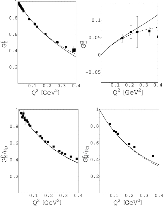
Figure 12: The Sachs form factors of the nucleon in manifestly Lorentz-invariant chiral perturbation theory at ${\cal O}(q^{4})$ including vector mesons as explicit degrees of freedom. Full lines: results in the extended on-mass-shell scheme; dashed lines: results in infrared regularization. The experimental data are taken from ref. Friedrich:2003iz .

Including the vector-meson degrees of freedom along the lines of refs. Fuchs:2003sh ; Schindler:2003xv generates the additional diagrams of fig. 11. The results for the Sachs form factors including vector-meson degrees of freedom are shown in fig. 12. As expected on phenomenological grounds Kubis:2000zd , the quantitative description of the data has improved considerably for $Q^{2}\geq 0.1$ GeV². The small difference between the two renormalization schemes is due to the way how the regular higher-order terms of loop integrals are treated. Note that on an absolute scale the differences between the two schemes are comparable for both $G_{E}^{p}$ and $G_{E}^{n}$. Numerically, the results are similar to those of ref. Kubis:2000zd . Due to the renormalization condition, the contribution of the vector-meson loop diagrams either vanishes (infrared renormalization scheme) or turns out to be small (EOMS). Thus, in hindsight our approach puts the traditional phenomenological vector-meson dominance model on a more solid theoretical basis.

4 Summary

Chiral perturbation theory is a cornerstone of our understanding of the strong interactions at low energies. Mesonic chiral perturbation theory has been tremendously successful and may be considered as a full-grown and mature area of low-energy particle physics. The apparent conflict between the determination of the ${\cal O}(q^{4})$ low-energy constants $(\bar{l}_{6}-\bar{l}_{5})$ from radiative pion beta decay on the one hand and the polarizability measurement on the other hand certainly requires additional work, in particular, from the theoretical side.

The impact on baryonic chiral perturbation theory due to the investigation of electromagnetic reactions at MAMI such as elastic electron-nucleon scattering, (virtual) Compton scattering and the electromagnetic production of pions cannot be overestimated. The possibility of a consistent manifestly Lorentz-invariant approach in combination with the rigorous inclusion of (axial-) vector-meson degrees of freedom and of the $\Delta(1232)$ resonance open the door to an application of ChPT in an extended kinematic region.

I would like to thank the organizers—HartmuthArenhövel, Hartmut Backe, Dieter Drechsel, Jörg Friedrich, Karl-Heinz Kaiser and Thomas Walcher—of the symposium 20 Years of Physics at the Mainz Microtron MAMI and express my best wishes for the future.

References

- (1) S. Weinberg, Physica A 96 (1979) 327.
- (2) J. Gasser and H. Leutwyler, Annals Phys. 158 (1984) 142.
- (3) J. Gasser and H. Leutwyler, Nucl. Phys. B 250 (1985) 465.
- (4) J. Gasser, M. E. Sainio and A. Švarc, Nucl. Phys. B 307 (1988) 779.
- (5) G. Ecker, arXiv:hep-ph/0507056.
- (6) S. Scherer, in Advances in Nuclear Physics, Vol. 27, edited by J. W. Negele and E. W. Vogt (Kluwer Academic/Plenum, New York 2003) 277-538.
- (7) S. Scherer and M. R. Schindler, arXiv:hep-ph/0505265.
- (8) E. Jenkins and A. V. Manohar, Phys. Lett. B 255 (1991) 558.
- (9) V. Bernard, N. Kaiser, J. Kambor and U.-G. Meißner, Nucl. Phys. B 388 (1992) 315.
- (10) V. Bernard, N. Kaiser and U.-G. Meißner, Int. J. Mod. Phys. E 4 (1995) 193.
- (11) G. Ecker and M. Mojžiš, Phys. Lett. B 365 (1996) 312.
- (12) N. Fettes, U.-G. Meißner, M. Mojžiš and S. Steininger, Annals Phys. 283 (2000) 273 [Erratum-ibid. 288 (2001) 249].
- (13) V. Bernard, N. Kaiser and U.-G. Meißner, Nucl. Phys. A 611 (1996) 429.
- (14) H. B. Tang, arXiv:hep-ph/9607436.
- (15) P. J. Ellis and H. B. Tang, Phys. Rev. C 57 (1998) 3356.
- (16) T. Becher and H. Leutwyler, Eur. Phys. J. C 9 (1999) 643.
- (17) M. F. M. Lutz, Nucl. Phys. A 677 (2000) 241.
- (18) J. Gegelia and G. Japaridze, Phys. Rev. D 60 (1999) 114038.
- (19) J. Gegelia, G. Japaridze and X. Q. Wang, J. Phys. G 29 (2003) 2303.
- (20) M. F. M. Lutz and E. E. Kolomeitsev, Nucl. Phys. A 700 (2002) 193.
- (21) T. Fuchs, J. Gegelia, G. Japaridze and S. Scherer, Phys. Rev. D 68 (2003) 056005.
- (22) S. Coleman, J. Math. Phys. 7 (1966) 787.
- (23) J. Goldstone, Nuovo Cim. 19 (1961) 154.
- (24) J. Goldstone, A. Salam and S. Weinberg, Phys. Rev. 127 (1962) 965.
- (25) D. Issler, SLAC-PUB-4943-REV (1990) (unpublished).
- (26) R. Akhoury and A. Alfakih, Annals Phys. 210 (1991) 81.
- (27) S. Scherer and H. W. Fearing, Phys. Rev. D 52 (1995) 6445.
- (28) H. W. Fearing and S. Scherer, Phys. Rev. D 53 (1996) 315.
- (29) J. Bijnens, G. Colangelo, and G. Ecker, J. High Energy Phys. 9902 (1999) 020.
- (30) T. Ebertshäuser, H. W. Fearing, and S. Scherer, Phys. Rev. D 65 (2002) 054033.
- (31) J. Bijnens, L. Girlanda, and P. Talavera, Eur. Phys. J. C 23 (2002) 539.
- (32) S. Weinberg, The Quantum Theory of Fields. Vol. 1: Foundations ( Cambridge University Press, Cambridge 1995) Chapter 12.
- (33) J. Bijnens and F. Cornet, Nucl. Phys. B 296 (1988) 557.
- (34) M. V. Terent’ev, Sov. J. Nucl. Phys. 16, 87 (1973) [Yad. Fiz. 16, 162 (1972)].
- (35) E. Frlež et al., Phys. Rev. Lett. 93 (2004) 181804.
- (36) U. Bürgi, Phys. Lett. B 377 (1996) 147.
- (37) U. Bürgi, Nucl. Phys. B 479 (1996) 392.
- (38) J. Bijnens, G. Colangelo, G. Ecker, J. Gasser and M. E. Sainio, Phys. Lett. B 374 (1996) 210.
- (39) J. Bijnens and P. Talavera, Nucl. Phys. B 489 (1997) 387.
- (40) C. Q. Geng, I. L. Ho and T. H. Wu, Nucl. Phys. B 684 (2004) 281.
- (41) Y. M. Antipov et al., Phys. Lett. B 121 (1983) 445.
- (42) T. A. Aibergenov et al., Czech. J. Phys. B 36 (1986) 948.
- (43) J. Ahrens et al., Eur. Phys. J. A 23 (2005) 113.
- (44) PLUTO Collaboration (C. Berger et al.), Z. Phys. C 26 (1984) 199.
- (45) DM1 Collaboration (A. Courau et al.), Nucl. Phys. B 271 (1986) 1.
- (46) DM2 Collaboration (Z. Ajaltoni et al.), in Proceedings of the VII International Workshop on Photon-Photon Collisions, Paris, 1-5 April 1986, edited by A. Courau, P. Kessler (World Scientific, Singapore, 1986).
- (47) MARK II Collaboration (J. Boyer et al.), Phys. Rev. D 42 (1990) 1350.
- (48) D. Drechsel and L. V. Fil’kov, Z. Phys. A 349 (1994) 177.
- (49) G. F. Chew and F. E. Low, Phys. Rev. 113 (1959) 1640.
- (50) C. Unkmeir, PhD Thesis, Johannes Gutenberg-Universität, Mainz (2000).
- (51) L. V. Fil’kov and V. L. Kashevarov, Eur. Phys. J. A 5 (1999) 285.
- (52) C. Hacker, N. Wies, J. Gegelia and S. Scherer, Phys. Rev. C 72 (2005) 055203.
- (53) C. Unkmeir, S. Scherer, A. I. L’vov and D. Drechsel, Phys. Rev. D 61 (2000) 034002.
- (54) T. Fuchs, B. Pasquini, C. Unkmeir and S. Scherer, Czech. J. Phys. 52 (2002) B135.
- (55) A. I. L’vov, S. Scherer, B. Pasquini, C. Unkmeir and D. Drechsel, Phys. Rev. C 64 (2001) 015203.
- (56) C. Unkmeir, A. Ocherashvili, T. Fuchs, M. A. Moinester and S. Scherer, Phys. Rev. C 65 (2002) 015206.
- (57) L. Ametller, J. Bijnens, A. Bramon and F. Cornet, Phys. Lett. B 276 (1992) 185.
- (58) P. Ko, Phys. Lett. B 349 (1995) 555.
- (59) S. Bellucci and C. Bruno, Nucl. Phys. B 452 (1995) 626.
- (60) A. A. Bel’kov, A. V. Lanyov and S. Scherer, J. Phys. G 22 (1996) 1383.
- (61) M. Jetter, Nucl. Phys. B 459 (1996) 283.
- (62) J. Bijnens, A. Fayyazuddin and J. Prades, Phys. Lett. B 379 (1996) 209.
- (63) E. Oset, J. R. Pelaez and L. Roca, Phys. Rev. D 67 (2003) 073013.
- (64) S. Prakhov et al., Phys. Rev. C 72 (2005) 025201.
- (65) J. Gasser and H. Leutwyler, Nucl. Phys. B 250 (1985) 539.
- (66) H. Leutwyler, Phys. Lett. B 374 (1996) 181.
- (67) R. Baur, J. Kambor and D. Wyler, Nucl. Phys. B 460 (1996) 127.
- (68) G. Knöchlein, S. Scherer and D. Drechsel, Phys. Rev. D 53 (1996) 3634.
- (69) B. M. K. Nefkens et al., Phys. Rev. C 72 (2005) 035212.
- (70) J. Wess and B. Zumino, Phys. Lett. B 37 (1971) 95.
- (71) E. Witten, Nucl. Phys. B 223 (1983) 422.
- (72) I. Giller, A. Ocherashvili, T. Ebertshäuser, M. A. Moinester and S. Scherer, Eur. Phys. J. A 25 (2005) 229.
- (73) D. Drechsel and L. Tiator, J. Phys. G 18 (1992) 449.
- (74) S. L. Adler and F. J. Gilman, Phys. Rev. 152 (1966) 1460.
- (75) V. Bernard, N. Kaiser and U. G. Meissner, Phys. Rev. Lett. 69 (1992) 1877.
- (76) S. Scherer and J. H. Koch, Nucl. Phys. A 534 (1991) 461.
- (77) A. Liesenfeld et al. [A1 Collaboration], Phys. Lett. B 468 (1999) 20.
- (78) D. Baumann, PhD Thesis, Johannes Gutenberg-Universität, Mainz (2004).
- (79) H. Haberzettl, Phys. Rev. Lett. 85 (2000) 3576.
- (80) T. Fuchs and S. Scherer, Phys. Rev. C 68 (2003) 055501.
- (81) H. Arenhövel and D. Drechsel, Nucl. Phys. A 233 (1974) 153.
- (82) P. A. M. Guichon, G. Q. Liu and A. W. Thomas, Nucl. Phys. A 591 (1995) 606.
- (83) S. Scherer, A. Y. Korchin and J. H. Koch, Phys. Rev. C 54 (1996) 904.
- (84) D. Drechsel, G. Knöchlein, A. Metz and S. Scherer, Phys. Rev. C 55 (1997) 424.
- (85) D. Drechsel, G. Knöchlein, A. Y. Korchin, A. Metz and S. Scherer, Phys. Rev. C 57 (1998) 941.
- (86) J. Roche et al. [VCS Collaboration], Phys. Rev. Lett. 85 (2000) 708.
- (87) G. Laveissiere et al. [Jefferson Lab Hall A Collaboration], Phys. Rev. Lett. 93 (2004) 122001.
- (88) H. Fonvieille, Prog. Part. Nucl. Phys. 55 (2005) 198.
- (89) B. Pasquini, M. Gorchtein, D. Drechsel, A. Metz and M. Vanderhaeghen, Eur. Phys. J. A 11 (2001) 185.
- (90) D. Drechsel, B. Pasquini and M. Vanderhaeghen, Phys. Rept. 378 (2003) 99.
- (91) A. Metz and D. Drechsel, Z. Phys. A 356 (1996) 351.
- (92) M. Vanderhaeghen, Phys. Lett. B 368 (1996) 13.
- (93) T. R. Hemmert, B. R. Holstein, G. Knöchlein and S. Scherer, Phys. Rev. Lett. 79 (1997) 22.
- (94) B. Pasquini, S. Scherer and D. Drechsel, Phys. Rev. C 63 (2001) 025205.
- (95) A. I. L’vov and S. Scherer (in preparation).
- (96) J. Gegelia, G. S. Japaridze and K. S. Turashvili, Theor. Math. Phys. 101 (1994) 1313 [Teor. Mat. Fiz. 101 (1994) 225].
- (97) M. R. Schindler, J. Gegelia and S. Scherer, Nucl. Phys. B 682 (2004) 367.
- (98) T. Fuchs, M. R. Schindler, J. Gegelia and S. Scherer, Phys. Lett. B 575 (2003) 11.
- (99) M. R. Schindler, J. Gegelia and S. Scherer, Phys. Lett. B 586 (2004) 258.
- (100) T. Fuchs, J. Gegelia and S. Scherer, Eur. Phys. J. A 19 (2004) 35.
- (101) B. C. Lehnhart, J. Gegelia and S. Scherer, J. Phys. G 31 (2005) 89.
- (102) T. Fuchs, J. Gegelia and S. Scherer, J. Phys. G 30 (2004) 1407.
- (103) M. R. Schindler, J. Gegelia and S. Scherer, Eur. Phys. J. A 26 (2005) 1.
- (104) B. Kubis and U.-G. Meißner, Nucl. Phys. A 679 (2001) 698.
- (105) J. Friedrich and Th. Walcher, Eur. Phys. J. A 17 (2003) 607.