Automated Calculation Scheme for $\alpha^{n}$ Contributions of QED to Lepton $g\!-\!2$: Generating Renormalized Amplitudes for Diagrams without Lepton Loops

Abstract

Among 12672 Feynman diagrams contributing to the electron anomalous magnetic moment at the tenth order, 6354 are the diagrams having no lepton loops, i.e., those of quenched type. Because the renormalization structure of these diagrams is very complicated, some automation scheme is inevitable to calculate them. We developed an algorithm to write down FORTRAN programs for numerical evaluation of these diagrams, where the necessary counterterms to subtract out ultraviolet subdivergence are generated according to Zimmermann’s forest formula. Thus far we have evaluated crudely integrals of 2232 tenth-order vertex diagrams which require vertex renormalization only. Remaining 4122 diagrams, which have ultraviolet-divergent self-energy subdiagrams and infrared-divergent subdiagrams, are being evaluated by giving small mass $\lambda$ to photons to control the infrared problem.

I Introduction

The anomalous magnetic moment of the electron, also called the electron $g\!-\!2$, is one of the most fundamental quantities of particle physics. Since its discovery in 1947 kusch it has been measured with steadily increasing precision rich ; VanDyck:1987ay . The best values of $g\!-\!2$ of the electron and the positron available in the literature VanDyck:1987ay

$$a_{e^{-}}({\rm exp}) =1\ 159\ 652\ 188.4\ (4.3)\times 10^{-12}\,,$$ (1)

$$a_{e^{+}}({\rm exp}) =1\ 159\ 652\ 187.9\ (4.3)\times 10^{-12}$$

were obtained by the Penning trap experiment. Here $a_{e}\equiv\frac{1}{2}(g-2)$ and the numerals in each parenthesis represent uncertainty in the last few digits of the respective values. The consistency of $a_{e^{-}}$ with $a_{e^{+}}$ in (1) within the experimental accuracy exhibits that CPT is a very good symmetry of the universe.

At present a new experiment is being carried out by a Harvard group using a new trap with cylindrical cavity Gabrielse , which is capable of controlling the electron–cavity-wall resonance with the help of analytical calculation brown . This experiment will reduce the measurement uncertainty of (1) substantially. It will enable us to test the validity of QED to a very high degree and to determine the fine structure constant $\alpha$ to an unprecedented precision of $7\times 10^{-10}$ or better, which is an order of magnitude better than the best non-QED value available at present wicht .

Of course, such a feat requires availability of theoretical calculation of matching precision. Within the framework of the Standard Model the QCD and weak interaction parts of the corrections to $a_{e}$ are known to be so small that their uncertainties do not affect the determination of $\alpha$ even with the expected precision of the new Harvard experiment. The uncertainties due to the QED contributions induced by the virtual propagation of muon and tau-lepton beginning at the fourth-order ($\alpha^{2}$) are also known to be negligible within the current precision. Thus the electron $g\!-\!2$ within the experimental precision of our current interest is determined almost entirely by the electron-photon interaction and can be regarded as a function of $\alpha$ alone.

The latest evaluation of $a_{e}$ in the Standard Model, including the hadronic vacuum polarization contribution, hadronic light-by-light-scattering contribution, the electroweak effect, and small QED contribution from virtual muon and tau-lepton loops is kn2

$$a_{e}=1\ 159\ 652\ 175.86\ (0.10)\ (0.26)\ (8.48)\times 10^{-12}\,,$$ (2)

where the uncertainties stem from (i) the remaining numerical uncertainty of the $\alpha^{4}$-term kn2 , (ii) the crudely estimated uncertainty of the $\alpha^{5}$-term CODATA:2002 , and (iii) that of the best non-QED $\alpha$ available at present, which is measured by the atom interferometry wicht combined with the cesium $D_{1}$ line measurement by the frequency comb technique udem ,

$$\alpha^{-1}(h/M_{{\rm Cs}})=137.036\ 000\ 3\ (10)\quad[7.4\ {\rm ppb}]\,.$$ (3)

An important byproduct of the study of the electron $g\!-\!2$ is that a more precise $\alpha$ can be obtained by combining the measurement (1) and the theory of $a_{e}$, which yields kn2

$$\alpha^{-1}(a_{e})=137.035\ 998\ 834\ (12)\ (31)\ (502)\quad[3.7\ {\rm ppb}]\,,$$ (4)

where the uncertainties $12$ and $31$ are due to the $\alpha^{4}$ and $\alpha^{5}$ terms, and $502$ comes from the experiment (1). The new Harvard experiment of $a_{e}$ is expected to reach a precision an order of magnitude better than that of (1). The $\alpha^{5}$ term will then become the largest source of unresolved systematic errors for obtaining $\alpha$ from $a_{e}$. Thus an explicit evaluation of the $\alpha^{5}$ term is urgently needed for further improvement of $\alpha(a_{e})$.

The pure QED contribution can be written as

$$a_{e}({\rm QED})=A_{1}^{(2)}\left(\frac{\alpha}{\pi}\right)+A_{1}^{(4)}\left(\frac{\alpha}{\pi}\right)^{2}+A_{1}^{(6)}\left(\frac{\alpha}{\pi}\right)^{3}+A_{1}^{(8)}\left(\frac{\alpha}{\pi}\right)^{4}+\cdots\,.$$ (5)

The coefficients are evaluated by the perturbation theory. By now the first four of them have been obtained kn2 :

$$A_{1}^{(2)\phantom{0}} =\phantom{-}0.5\,,$$ (6)

$$A_{1}^{(4)\phantom{0}} =-0.328\ 478\ 965\cdots\,,$$

$$A_{1}^{(6)\phantom{0}} =\phantom{-}1.181\ 241\ 456\cdots\,,$$

$$A_{1}^{(8)\phantom{0}} =-1.728\ 3\ (35)\,.$$

$A_{1}^{(10)}$ has not yet been evaluated. An educated guess is that it may be found within the range $(-3.8,3.8)$ CODATA:2002 .

The first theoretical calculation of $a_{e}$ was carried out analytically by Schwinger in 1948 schwinger . The number of Feynman diagrams involved was just one in this case. The excellent agreement of his calculation with the measurement kusch was one of the pivotal triumphs of renormalization theory of QED, which was just being developed. Refinement of theory to the fourth-order involves seven Feynman diagrams. It took more than 7 years before the analytic value of $A_{1}^{(4)}$ was obtained in 1957 som-pet . Analytic evaluation of $A_{1}^{(6)}$ is far more challenging requiring evaluation of 72 Feynman diagrams. It took effort of many physicists and many years of hard work and was completed only in 1996 lap-rem .

The numerical evaluation scheme was developed by one of the authors (T. K.) and Cvitanović for the evaluation of the sixth-order contribution Cvitanovic:1974uf ; Cvitanovic:1974sv ; Cvitanovic:1974um and extended later to the eighth-order kl1 . Up to now $A_{1}^{(8)}$ was calculated only numerically, which involves the evaluation of 891 Feynman diagrams. Although the initial crude result was published in 1974 kl1 , improvement of numerical precision required many years of extensive computation and the final result was published only recently kn2 . From the viewpoint of obtaining $A_{1}^{(10)}$ the numerical integration approach is the only practical choice at present.

The contribution to the $\alpha^{5}$ term of the electron $g\!-\!2$ comes from $12672$ vertex-type Feynman diagrams, which can be categorized into 6 sets according to their structures and classified further into 32 gauge-invariant subsets. See Appendix A and Ref. kn3 for the details of classification. Most subsets that contain closed lepton loops have relatively simple structure and are calculable by a slight extension of the method developed in Refs. Cvitanovic:1974um and kl1 . As far as the muon $g\!-\!2$ is concerned, they cover the subsets that give rise to the leading contributions. Thus far 17 of 32 subsets have been evaluated and reported in Refs. kino1 and kn-radcor05 . Detail of these works is presented in Ref. kn3 .

For the electron $g\!-\!2$, however, none of 32 subsets is dominant so that all must be evaluated. A particularly difficult one is Set V, a huge set consisting of 6354 vertex diagrams, all of which have pure radiative corrections and no closed lepton loops (see Fig. 12 in Appendix A). Throughout this paper these diagrams will be referred to as “quenched-type (q-type)” since they are analogous to the so-called quenched diagrams of QCD. The difficulty of Set V stems from the fact that many of them have very large number of ultraviolet (UV) and infrared (IR) divergences. This makes the previous approach highly impractical since it runs into an extremely sever logistic problem. Unless this is solved, it will be close to impossible for mortals to deal with Set V and hence the entire tenth-order electron $g\!-\!2$ without making mistake.

The purpose of this paper is to present our solution to this very difficult problem. We have developed a scheme of automatic code generation which enables us to generate renormalized integrals for all diagrams of Set V with a breathtaking speed. Outputs of this code are ready to be integrated by numerical means.

We begin by exploiting the equation derived from the Ward-Takahashi identity, which relates the sum of a set of vertex diagrams to a self-energy-like diagram Cvitanovic:1974um . This relation together with the time-reversal invariance of QED enables us to reduce the number of independent integrals of Set V diagrams drastically from 6354 to 389. The method starting from the Ward-Takahashi (W-T) summed diagrams is called Version A, while the conventional approach by vertex diagrams is referred to as Version B for the sake of distinction kn1 .

The systematic scheme for constructing numerical integration code consists of the following steps.

1. Identify the diagrams contributing to the electron $g\!-\!2$ and their UV- and IR-divergent subdiagrams.

2. Carry out momentum space integration exactly using a home-made integration table and convert it into an integral over Feynman parameters. The result is expressed symbolically as a function of quantities $U$, $B_{ij}$, and $A_{j}$, which are homogeneous polynomials of Feynman parameters. We call them building blocks.

3. Find the explicit forms of $U$ and $B_{ij}$ which are determined from the topological structure of the Feynman diagram ${\cal G}$ obtained by removing all external lines and disregarding the distinction between an electron line and a photon line.

4. To prepare for numerical integration on computer UV and IR divergences must be removed from the integrand beforehand. In Ref. Cvitanovic:1974um a regularization scheme was developed in which divergences are eliminated by point-by-point subtraction by counterterms which are derived from the original integrand by simple power-counting rules. This scheme is denoted as K-operation for the UV divergence and I-operation for the IR divergence Cvitanovic:1974sv ; Kinoshita_book .

5. Counterterms thus constructed can be identified with only the UV divergent parts of the renormalization constants so that the result of step (IV) is not fully equivalent to the standard on-shell renormalization. The difference between full renormalization and intermediate renormalization must therefore be evaluated by summing up all subtraction terms.

The scheme (I)–(V) itself is completely general and applicable to any order of perturbation. Step (II) was quite difficult already in the sixth-order and still harder in the eighth-order. It was carried out entirely by computer with the help of algebraic manipulation programs such as SCHOONSCHIP veltman and FORM vermaseren . Steps (I), (III), (IV) and (V) were simple enough in the sixth-order case and still manageable in the eighth-order case to be executed by hand manipulation.

It is evident, however, that such a pedestrian approach is no longer adequate for the calculation of the tenth-order diagrams so that a highly automated approach is required. This applies not only to the step (II) but to all other steps. It turns out that the automation scheme can be formulated quite efficiently for the q-type diagrams by making full use of their inherent properties. For Step (I) a systematic procedure for the generation of diagrams and the identification of UV divergent subdiagrams is possible. The graph-theoretical notions are easily identified for this type of diagrams, which enables the automated construction of topological quantities in Step (III).

The UV subtractions in Step (IV) can be organized by following the Zimmermann’s forests of subdiagrams exactly Zimmermann:1969jj . The forests are constructed as combinations of subdiagrams identified in Step (I).

This enables us to write a code which controls all steps (I), (II), (III), and (IV) automatically. Namely, we have obtained a code which turns an input of single-line information characterizing the structure of a Feynman diagram into a fully renormalized Feynman parametric integral.

Thus far we have obtained FORTRAN codes of renormalized integrals for 2232 vertex diagrams which contain vertex renormalization subdiagrams only. Crude evaluation by the Monte-Carlo integration routine VEGAS lepage shows that our scheme works well as expected.

The next step is to evaluate the remaining 4122 diagrams which have self-energy subdiagrams. These diagrams have also IR divergences. The simplest way to deal with the IR problem is to give a small mass $\lambda$ to photons, which can be implemented with a minor extension of the automating code. Of course, the numerical result will have an uncertainty of order $\lambda$. It may also suffer from non-negligible digit-deficiency problem commonly encountered in numerical integration kn1 . Nevertheless it will be good enough for getting crude values of $A_{1}^{(10)}$ so that we follow this approach as the first step.

This scheme has thus far been tested successfully with the sixth-order q-type diagrams and reproduced the analytic result after proper treatment of residual renormalization terms. The next step is to check the eighth-order q-type diagrams, which is numerically known. It seems successful so far except for a few diagrams which have severe IR divergences. Those diagrams may require minor modifications to the present automation code. After these exercises we will tackle the tenth-order problem.

To obtain a result independent of $\lambda$ it is necessary to extend the automating code to include IR subtraction terms constructed in a manner similar to that of UV counterterms. To complete this calculation we must evaluate the contribution of residual renormalization terms, which consists of integrals of up to eighth-order for 6804 UV-divergent subdiagrams. The result of these works will be reported in the subsequent papers.

This paper is organized as follows. In Section II we briefly review the parametric integral formalism to obtain the anomalous magnetic moment of leptons in Version A approach. In Section III we describe K-operation for the subtraction of UV divergence which derives from a single UV-divergent subdiagram. We then proceed to the case involving more than one subdiagram in Section IV in relation to the forest structures. It is one of the essential ingredients for our automated scheme. In Section V and VI we focus on a specific type of diagrams, namely, q-type diagrams. We discuss their intrinsic properties in Section V. We see in Section VI that use of these properties allows us to develop algorithms to identify UV divergences in terms of all relevant forests. It enables us to construct the renormalized amplitude in an automated manner. In Section VII we show the whole flow of our automated scheme in detail. Section VIII is devoted to the conclusion and discussions. In Appendix A we show the classification of diagrams that contribute to $A_{1}^{(10)}$. Appendix B contains useful formulae for computing the basic building blocks of the Feynman integrals which can be readily adapted to the programming languages such as C++ and FORTRAN.

II General Formalism

In this section we present the general formalism for evaluating QED contribution of anomalous magnetic moment of lepton in perturbation theory. It is a brief summary of the literature Cvitanovic:1974um ; Kinoshita_book , which is included here to provide concrete prescription of formulation for our automation scheme presented in the latter part of this paper, and also to make this article self-contained.

II.1 Anomalous magnetic moment of lepton

The magnetic property of a lepton can be studied through examining its scattering by a static magnetic field. The amplitude of this process including interactions with the virtual photon fields can be represented as follows, by taking account of the gauge symmetry, invariances under Lorentz, C, P, and T transformations:

$$e\bar{u}(p^{\prime\prime})\left[\gamma^{\mu}\,F_{1}(q^{2})+\frac{i}{2m}\sigma^{\mu\nu}\,q_{\nu}\,F_{2}(q^{2})\right]u(p^{\prime})\,A_{\mu}^{\,e}(\vec{q})\,,$$ (7)

where $p^{\prime}=p-q/2$, $p^{\prime\prime}=p+q/2$, $q=p^{\prime\prime}-p^{\prime}$ and $\sigma^{\mu\nu}=\frac{i}{2}(\gamma^{\mu}\gamma^{\nu}-\gamma^{\nu}\gamma^{\mu})$. $A_{\mu}^{\,e}$ is the vector potential of the external static magnetic field. $F_{1}$ and $F_{2}$ are called the charge and magnetic form factors, respectively, and the charge form factor is normalized so that $F_{1}(0)=1$.

The anomalous magnetic moment $a_{e}$ is the static limit of the magnetic form factor $F_{2}(q^{2})$, and it is expressed as

$$a_{e}=F_{2}(0)=Z_{2}M$$ (8)

with

$$M=\lim_{q^{2}\to 0}{\rm Tr}\bigl{(}P_{\nu}(p,q)\,\Gamma^{\nu}\bigr{)}\,,$$ (9)

where $Z_{2}$ is the wave function renormalization constant, $\Gamma^{\nu}$ is the proper vertex part, and $P_{\nu}(p,q)$ is the magnetic projection operator,

$$P^{\nu}(p,q)=\frac{1}{4p^{4}q^{2}}\left({/\hskip-5.50003pt{}p}{}-\frac{1}{2}{/\hskip-5.50003pt{}q}{}+m\right)\left[m\gamma^{\nu}p^{2}-\left(m^{2}+\frac{1}{2}q^{2}\right)p^{\nu}\right]\left({/\hskip-5.50003pt{}p}{}+\frac{1}{2}{/\hskip-5.50003pt{}q}{}+m\right)\,.$$ (10)

Here, the momentum of incoming lepton $p-\frac{1}{2}q$ and that of outgoing lepton $p+\frac{1}{2}q$ are on the mass shell so that $p$ and $q$ satisfy $p^{2}=m^{2}-\frac{1}{4}q^{2}$ and $p\cdot q=0$.

We evaluate the anomalous magnetic moment $a_{e}$ in the framework of perturbation theory. Because of renormalizability of QED it can be written as a power series in $\frac{\alpha}{\pi}$ whose coefficients are finite and calculable quantities.

II.2 Construction of Feynman parametric integral

In perturbative analysis of QED the amplitude is usually expressed as an integral of loop momenta flowing through the Feynman diagram. In this paper we convert it into an integral of Feynman parameters $z_{i}$ assigned to internal lines aldins ; Cvitanovic:1974uf .

We consider a $2n$th-order lepton vertex diagram $\cal{G}$ which describes the scattering of an incoming lepton with momentum $p-q/2$ into an outgoing lepton with momentum $p+q/2$ by an external magnetic field. $\cal{G}$ consists of $2n\!+\!1$ interaction vertices connected by $2n$ lepton propagators and $n$ photon propagators, which are given in the form (in Feynman gauge):

$$i\frac{{/\hskip-5.50003pt{}p}{}_{i}+m_{i}}{p_{i}^{\ 2}-m_{i}^{\ 2}},\qquad\frac{-ig^{\mu\nu}}{p_{i}^{\ 2}-m_{i}^{\ 2}}\,,$$ (11)

respectively. The momentum $p_{i}$ may be decomposed as $p_{i}=k_{i}+q_{i}$, in which $k_{i}$ is a linear combination of loop momenta, while $q_{i}$ is a linear combination of external momenta. $m_{i}$ is the mass associated with the line $i$, which is temporarily distinguished from each other.

We introduce an operator $D_{i}^{\ \mu}$ by

$$D_{i}^{\ \mu}\equiv\frac{1}{2}\int_{m_{i}^{\ 2}}^{\infty}dm_{i}^{\ 2}\ \frac{\partial}{\partial q_{i\mu}}$$ (12)

and replace each numerator ${/\hskip-5.50003pt{}p}{}_{i}={/\hskip-5.50003pt{}k}{}_{i}+{/\hskip-5.50003pt{}q}{}_{i}$ of lepton propagators (11) by ${\hskip 1.99997pt/\hskip-7.5pt{}D}{}_{i}$. Since $D_{i}^{\ \mu}$ does not depend on $k_{i}$ explicitly, the numerators can be pulled out in front of the momentum integration as far as the integrand is adequately regularized.

The product of denominators are combined into one using the formula,

$$\prod_{i=1}^{N}\frac{1}{\chi_{i}}=(N-1)!\left[\prod_{i=1}^{N}\int_{0}^{1}\!dz_{i}\right]\delta\left(1-\sum_{i=1}^{N}z_{i}\right)\,\frac{1}{\displaystyle\left(\sum_{i=1}^{N}z_{i}\chi_{i}\right)^{N}}\,.$$ (13)

The sum $\sum_{i}z_{i}\chi_{i}$ is a quadratic form of loop momenta so that it can be integrated analytically. As a consequence the amplitude is converted into an integral over Feynman parameters $z_{i}$ which is expressed in a concise form as

$$\Gamma_{\cal{G}}^{\ \nu}=\biggl{(}\frac{1}{4}\biggr{)}^{n}(n-1)!\ \mathbb{F}^{\nu}\!\int(dz)_{\cal{G}}\,\frac{1}{U^{2}V^{n}}\,,$$ (14)

where $N=3n$ and

$$(dz)_{\cal G}=\prod_{i=1}^{N}dz_{i}\ \delta\left(1-\sum_{i=1}^{N}z_{i}\right)\,,$$ (15)

$$V=\sum_{i=1}^{N}z_{i}(m_{i}^{\ 2}-q_{i}\cdot Q^{\prime}_{i})\,,$$ (16)

$$Q^{\prime\ \mu}_{i}=-\frac{1}{U}\sum_{j=1}^{N}\ q_{j}^{\ \mu}z_{j}B^{\prime}_{ij}\,,$$ (17)

$$B^{\prime}_{ij}=B_{ij}-\delta_{ij}\frac{U}{z_{j}}\,.$$ (18)

In Eq. (14) we have omitted the factor $(\alpha/\pi)^{n}$ for simplicity. $U$ and $B_{ij}$ are homogeneous polynomials of degree $n$ and $n-1$ in Feynman parameters $\{z_{i}\}$, respectively. Their precise definitions are given in later sections. The operator $\mathbb{F}^{\nu}$ is of the form

$$\mathbb{F}^{\nu}=\gamma^{\alpha_{1}}({\hskip 1.99997pt/\hskip-7.5pt{}D}{}_{1}+m_{1})\gamma^{\alpha_{2}}\dots\gamma^{\nu}\dots\gamma^{\alpha_{2n-1}}({\hskip 1.99997pt/\hskip-7.5pt{}D}{}_{2n}+m_{2n})\gamma^{\alpha_{2n}}\prod_{k=1}^{n}g_{\alpha_{i_{k}}\alpha_{j_{k}}}\,,$$ (19)

where $\prod_{k}g_{\alpha_{i_{k}}\alpha_{j_{k}}}$ is a diagram-specific product. If $\cal G$ has closed lepton loops $\mathbb{F}^{\nu}$ also contains appropriate trace operations.

Note that $\mathbb{F}^{\nu}$ can now be brought into the $z$-integral. The operator $D_{i}^{\ \mu}$ in $\mathbb{F}^{\nu}$ acts on $1/V^{n}$ as

$$D_{i}^{\ \mu}\frac{1}{V^{n}}=\frac{Q^{\prime\,\mu}_{i}}{V^{n}}\,,$$ (20)

$$D_{i}^{\ \mu}D_{j}^{\ \nu}\frac{1}{V^{n}}=\frac{Q^{\prime\,\mu}_{i}Q^{\prime\,\nu}_{j}}{V^{n}}-\frac{1}{2(n-1)}\frac{g^{\mu\nu}B^{\prime}_{ij}}{UV^{n-1}}\,,$$ (21)

$$D_{i}^{\ \mu}D_{j}^{\ \nu}D_{k}^{\ \rho}\frac{1}{V^{n}}=\frac{Q^{\prime\,\mu}_{i}Q^{\prime\,\nu}_{j}Q^{\prime\,\rho}_{k}}{V^{n}}$$

$$\qquad-\frac{1}{2(n-1)}(g^{\mu\nu}B^{\prime}_{ij}Q^{\prime\,\rho}_{k}+g^{\nu\rho}B^{\prime}_{jk}Q^{\prime\,\mu}_{i}+g^{\rho\mu}B^{\prime}_{ki}Q^{\prime\,\nu}_{j})\frac{1}{UV^{n-1}}\,,$$ (22)

$$\dots\,.$$

The result of this operation may be summarized as a set of rules for a string of operators $D_{i}^{\ \mu}$:

• when ${\hskip 1.99997pt/\hskip-7.5pt{}D}{}_{i}$ and ${\hskip 1.99997pt/\hskip-7.5pt{}D}{}_{j}$ are “contracted”, they are turned into a pair of $\gamma^{\mu}$ and $\gamma_{\mu}$ times a factor $(-\frac{1}{2}B^{\prime}_{ij})$.

• uncontracted $D_{i}$ is replaced by $Q^{\prime}_{i}$.

As a consequence the action of $\mathbb{F}^{\nu}$ produces a series of terms of the form

$$\mathbb{F}^{\nu}\frac{1}{U^{2}V^{n}}=\frac{F_{0}^{\nu}}{U^{2}V^{n}}+\frac{F_{1}^{\nu}}{U^{3}V^{n-1}}+\cdots\,,$$ (23)

where $F_{k}^{\nu}$ are polynomials of $B^{\prime}_{ij}$ and $Q^{\prime}_{i}$. The subscript $k$ denotes the number of contractions. $F_{k}^{\nu}$ also includes an overall factor $\dfrac{1}{(n-1)(n-2)\cdots(n-k)}$.

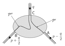
Figure 1: A vertex diagram with given external momenta. A choice of paths ${\cal P}^{\prime}$ and ${\cal P}^{\prime\prime}$ are shown.

It is convenient to replace vectors $Q^{\prime\,\mu}_{i}$ by scalar functions. Suppose the momentum $p^{\mu}-\dfrac{q^{\mu}}{2}$ enters the graph $\cal G$ at the point $A$, follows the path ${\cal P}^{\prime}={\cal P}(AC)$, and leaves at $C$, and $p^{\mu}+\dfrac{q^{\mu}}{2}$ enters at $C$, follows the path ${\cal P}^{\prime\prime}={\cal P}(CB)$, and leaves at $A$. (Fig. (1).) This can be expressed concisely by

$$q_{j}^{\ \mu}=\eta_{j{\cal P}^{\prime}}\left(p^{\mu}-\frac{q^{\mu}}{2}\right)+\eta_{j{\cal P}^{\prime\prime}}\left(p^{\mu}+\frac{q^{\mu}}{2}\right)\,,$$ (24)

where $\eta_{j{\cal P}^{\prime}}=(1,-1,0)$ according to whether the line $j$ lies (along, against, outside of) the path ${\cal P}^{\prime}$. Similarly for $\eta_{j{\cal P}^{\prime\prime}}$. Substituting Eq. (24) in Eq. (17) we obtain

$$Q^{\prime\mu}_{i}=A_{i}^{\,{\cal P}^{\prime}}\left(p^{\mu}-\frac{q^{\mu}}{2}\right)+A_{i}^{\,{\cal P}^{\prime\prime}}\left(p^{\mu}+\frac{q^{\mu}}{2}\right)\,,$$ (25)

where

$$A_{i}^{\,{\cal P}^{\prime}}=-\frac{1}{U}\sum_{j=1}^{N}\eta_{j{\cal P}^{\prime}}z_{j}B^{\prime}_{ji}\,.$$ (26)

Similarly for $A_{i}^{\,{\cal P}^{\prime\prime}}$. $A_{i}^{\,{\cal P}^{\prime}}$, $A_{i}^{\,{\cal P}^{\prime\prime}}$ will be called scalar currents associated with $p^{\mu}-\dfrac{q^{\mu}}{2}$, $p^{\mu}+\dfrac{q^{\mu}}{2}$, respectively.

If we choose a path ${\cal P}={\cal P}(AB)$ for $p^{\mu}$, the corresponding scalar current becomes $A_{i}^{\,{\cal P}}=A_{i}^{\,{\cal P}^{\prime}}+A_{i}^{\,{\cal P}^{\prime\prime}}$. Note that the choice of ${\cal P}(AB)$ is flexible as far as the end points $A$, $B$ are fixed. Note also that ${\cal P}(AB)$ no longer depends on $C$.

II.3 Building blocks, $B_{ij}$ and $U$

In our formalism, the parametric functions $B_{\alpha\beta}$ and $U$ provide the basic building blocks which are defined on the chain diagram corresponding to the diagram $\cal{G}$. Here $\alpha,\beta$ refer to the chains; a chain is a set of internal lines that carry the same loop momentum. The chain diagram is derived from $\cal{G}$ by amputating all the external lines and disregarding the distinction between the types of lines. Every chain is assumed to be properly directed. $B_{\alpha\beta}$ and $U$ are homogeneous polynomials of degree $n-1$ and $n$, respectively. They are the quantities that reflect the topological structure underlying the diagram $\cal{G}$.

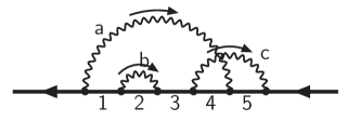
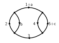
Figure 2: A diagram (left) and the chain diagram derived from it (right).

$B_{\alpha\beta}$ and $U$ can be obtained recursively by the following relations,

$$B_{\alpha\beta}=\sum_{c}\xi_{\alpha,c}\,\xi_{\beta,c}\,U_{{\cal G}/c}\,,$$ (27)

$$\xi_{\lambda,s}U=\sum_{\alpha}\xi_{\lambda,s}z_{\alpha}B_{\lambda\alpha},\qquad\text{for any $\lambda\in s$}\,,$$ (28)

starting from $U=\alpha$ for a single loop. Here the summation over $c$ runs over all self-nonintersecting closed loops on $\cal{G}$. The loop matrix $\xi_{\alpha,c}$ is a projector of chain $\alpha$ to the loop $c$, which takes $(1,-1,0)$ according to whether $\alpha$ is (along, against, outside of) $c$. $U_{{\cal G}/c}$ is the $U$ function for the reduced diagram ${\cal G}/c$ that is obtained from $\cal G$ by shrinking the loop $c$ to a point. The loop $s$ in Eq. (28) is an arbitrary closed loop.

Alternate and equivalent formulae for $B_{\alpha\beta}$ and $U$ are obtained in the following manner. Suppose a set of independent self-nonintersecting loops (called a fundamental set of circuits) is given and define $U_{st}$ by the summation over all chains by

$$U_{st}=\sum_{\alpha}z_{\alpha}\,\xi_{\alpha,s}\,\xi_{\alpha,t}\,,$$ (29)

where $s,t$ are labels of circuits in the set. Then, $U$ and $B_{\alpha\beta}$ are given by

$$U=\det_{st}U_{st}\,,$$ (30)

$$B_{\alpha\beta}=U\sum_{st}\xi_{\alpha,s}\,\xi_{\beta,t}\,(U^{-1})_{st}\,.$$ (31)

For a given diagram $\cal G$, first we have to identify the fundamental set of circuits, and construct the loop matrix $\xi_{\alpha,s}$. Then we can obtain $U$ and $B_{\alpha\beta}$ according to the formulae above.

$B_{ij}$ of the lines $i,j$ is identical with $B_{\alpha\beta}$ whose indices are such that $i\in\alpha$ and $j\in\beta$. $B_{ij}$ satisfies a so-called junction law on each vertex if the diagram ${\cal G}$ were regarded as an electric circuit in which the Feynman parameter $z_{i}$ corresponds to the resistance of the line $i$:

$$\sum_{i}\epsilon_{vi}B_{ij}=0$$ (32)

for any vertex $v$ and any internal line $j$, where $\epsilon_{vi}$ is called incident matrix defined by

$$\epsilon_{vi}=\begin{cases}1&\text{if the line $i$ enters the vertex $v$,}\\ -1&\text{if the line $i$ leaves the vertex $v$,}\\ 0&\text{otherwise.}\end{cases}$$ (33)

$B_{ij}$ also satisfies a loop-law given by the following relation for arbitrary closed loop $s$ and arbitrary line $j$:

$$\sum_{i}\xi_{i,s}\,z_{i}\,B^{\prime}_{ji}=0\,.$$ (34)

These relations reduce the number of independent elements among $B_{ij}$. It also provides consistency checks which are useful in the actual calculations.

II.4 $a_{e}$ from a set of vertex diagrams summed by Ward-Takahashi identity

A set of vertex diagrams which are derived from a self-energy diagram by inserting an external vertex in every lepton propagators share many properties. Actually we can even go further to relate those integrals to a single integral of the self-energy-like diagram through the Ward-Takahashi identity. This relation is useful when we consider higher order calculations because it reduces the number of independent integrals substantially.

It is well known that the proper vertex $\Gamma^{\mu}=\gamma^{\mu}+\Lambda^{\mu}$ and self-energy part $\Sigma$ are related by the Ward-Takahashi identity

$$q_{\mu}\Lambda^{\mu}=-\Sigma\left(p+\frac{1}{2}q\right)+\Sigma\left(p-\frac{1}{2}q\right)\,.$$ (35)

This relation holds perturbatively as well for $\Sigma_{\cal{G}}$ representing the lepton self-energy diagram $\cal{G}$ and the sum of vertex diagrams $\Lambda_{\cal{G}}$ that are obtained by inserting an external vertex into $\cal{G}$ in every possible way. Differentiating both sides of Eq. (35) with respect to $q^{\mu}$ and taking the static limit $q\to 0$ of the external magnetic field, we have

$$\Lambda^{\nu}(p,q)\simeq-q^{\mu}\biggl{[}\frac{\partial\Lambda_{\mu}(p,q)}{\partial q_{\nu}}\biggr{]}_{q=0}-\frac{\partial\,\Sigma(p)}{\partial p_{\nu}}\,.$$ (36)

We may evaluate $a_{e}$ starting from either side of this expression; a straightforward way is to calculate each vertex diagram individually and to gather them up according to the left-hand side (Version B approach in Ref. kn1 ), or else we can combine the set of vertices into one according to the right-hand side (Version A approach). We adopt Version A in the present study.

In the Feynman parametric form, the $2n$th-order magnetic moment associated with a self-energy-like diagram $\cal{G}$ can be written as Cvitanovic:1974um

$$M^{(2n)}=\left(\frac{-1}{4}\right)^{n}(n-1)!\int(dz)_{\cal{G}}\,\left[\frac{\mathbb{E}+\mathbb{C}}{n-1}\frac{1}{U^{2}V^{n-1}}+(\mathbb{N}+\mathbb{Z})\frac{1}{U^{2}V^{n}}\right]\,,$$ (37)

where $\mathbb{E}$, $\mathbb{C}$, $\mathbb{N}$, and $\mathbb{Z}$ are a set of operators defined as

$$\mathbb{N}=\frac{1}{4}{\rm Tr}\bigl{[}P_{1}^{\nu}p_{\nu}(2G\mathbb{F})\bigr{]}\,,$$ (38)

$$\mathbb{E}=\frac{1}{4}{\rm Tr}\bigl{[}P_{1}^{\nu}\mathbb{E}_{\nu}\bigr{]}\,,$$ (39)

$$\mathbb{C}=\frac{1}{4}{\rm Tr}\bigl{[}P_{2}^{\mu\nu}\mathbb{C}_{\mu\nu}\bigr{]}\,,$$ (40)

$$\mathbb{Z}=\frac{1}{4}{\rm Tr}\bigl{[}P_{2}^{\mu\nu}\mathbb{Z}_{\mu\nu}\bigr{]}\,.$$ (41)

The magnetic projectors $P_{1}^{\nu}$ and $P_{2}^{\mu\nu}$ are derived from Eq. (10) by averaging over the direction of $q_{\mu}$, and take the following forms:

$$P_{1}^{\nu}=\frac{1}{3}\gamma^{\nu}-\left(1+\frac{4}{3}\frac{{/\hskip-5.50003pt{}p}{}}{m}\right)\frac{p^{\nu}}{m}\,,$$ (42)

$$P_{2}^{\mu\nu}=\frac{1}{3}\left(1+\frac{{/\hskip-5.50003pt{}p}{}}{m}\right)\left(g^{\mu\nu}-\gamma^{\mu}\gamma^{\nu}+\frac{p^{\mu}}{m}\gamma^{\nu}-\frac{p^{\nu}}{m}\gamma^{\mu}\right)\,.$$ (43)

The operator $\mathbb{F}$ is the numerator part of the self-energy-like diagram $\cal{G}$ constructed in the similar form as Eq. (19):

$$\mathbb{F}=\gamma^{\alpha_{1}}({\hskip 1.99997pt/\hskip-7.5pt{}D}{}_{1}+m_{1})\gamma^{\alpha_{2}}\dots\gamma^{\alpha_{2n-1}}({\hskip 1.99997pt/\hskip-7.5pt{}D}{}_{2n-1}+m_{2n-1})\gamma^{\alpha_{2n}}\prod_{k=1}^{n}g_{\alpha_{i_{k}}\alpha_{j_{k}}}\,,$$ (44)

which may contain appropriate trace operations if $\cal G$ has closed lepton loops. The operator $\mathbb{E}^{\nu}$ is defined by

$$\mathbb{E}^{\nu}=\frac{\partial\,\mathbb{F}}{\partial p_{\nu}}=\sum_{\rm all\ leptons}A_{i}\mathbb{F}_{i}^{\ \nu}\,,$$ (45)

in which $\mathbb{F}_{i}^{\ \nu}$ is obtained from $\mathbb{F}$ by substituting in the $i$th line:

$$({\hskip 1.99997pt/\hskip-7.5pt{}D}{}_{i}+m_{i})\to\gamma^{\nu}\,.$$ (46)

The operator $\mathbb{Z}^{\mu\nu}$ is defined by

$$\mathbb{Z}^{\mu\nu}=\sum_{j}\mathbb{Z}_{j}^{\ \mu\nu}\,.$$ (47)

The sum runs only over the lepton lines into which the external photon line can be inserted. $\mathbb{Z}_{j}^{\ \mu\nu}$ is obtained from $\mathbb{F}$ by substituting in the $j$th line:

$$({\hskip 1.99997pt/\hskip-7.5pt{}D}{}_{j}+m_{j})\to\frac{1}{2}\bigl{[}\gamma^{\mu}\gamma^{\nu}({\hskip 1.99997pt/\hskip-7.5pt{}D}{}_{j}+m_{j})-({\hskip 1.99997pt/\hskip-7.5pt{}D}{}_{j}+m_{j})\gamma^{\nu}\gamma^{\mu}\bigr{]}\,.$$ (48)

The operator $\mathbb{C}^{\mu\nu}$ is defined by

$$\mathbb{C}^{\mu\nu}=\sum_{i<j}C_{ij}\mathbb{F}_{ij}^{\ \mu\nu}\,,$$ (49)

where $i$ and $j$ refer to all lepton lines. $C_{ij}$ is given by

$$C_{ij}=\frac{1}{U^{2}}\sum_{k<l}z_{k}z_{l}(B^{\prime}_{ik}B^{\prime}_{jl}-B^{\prime}_{il}B^{\prime}_{jk})\,,$$ (50)

where $k$, $l$ are taken from the lepton lines that belong to the path on which the momentum $q^{\nu}$ of the external magnetic field flows. $\mathbb{F}_{ij}^{\ \mu\nu}$ is obtained from $\mathbb{F}$ by substituting in the $i$th and $j$th lepton lines:

$$({\hskip 1.99997pt/\hskip-7.5pt{}D}{}_{i}+m_{i}),\ ({\hskip 1.99997pt/\hskip-7.5pt{}D}{}_{j}+m_{j})\to\gamma^{\mu},\ \gamma^{\nu}\,.$$ (51)

$G$ is given by

$$G=\sum_{i}z_{i}\,A_{i}\,,$$ (52)

where the summation runs over the lepton lines on which the external momentum $p^{\mu}$ flows (depending on the choice of path ${\cal P}(AB)$ for the scalar currents).

We can now construct the integrand in the following two steps.

1. Express the integrand as a function of symbols $B_{ij}$, $A_{i}$, $U$, $V$, and $C_{ij}$.

2. Express those building blocks explicitly in terms of the Feynman parameters $z_{i}$.

Step (I) can be achieved analytically by algebraic manipulation programs such as FORM vermaseren . All the integrals are generated from a small number of templates with the permutation of indices according to the specific structure of each diagram. Step (II) is performed along the prescriptions outlined above, once $B_{ij}$ and $U$ are obtained by the formulae in Section II.3. The magnetic moment contribution (37) now can be expressed as a parametric integral:

$$M^{(2n)}=\left(-\frac{1}{4}\right)^{n}(n-1)!\,\int(dz)_{\cal G} \left[\frac{1}{n-1}\left(\frac{E_{0}+C_{0}}{U^{2}V^{n-1}}+\frac{E_{1}+C_{1}}{U^{3}V^{n-2}}+\cdots\right)\right.$$ (53)

$$\quad+\left.\left(\frac{N_{0}+Z_{0}}{U^{2}V^{n}}+\frac{N_{1}+Z_{1}}{U^{3}V^{n-1}}+\cdots\right)\right]\,.$$

III Subtractive UV renormalization procedure

The amplitude thus far constructed in the previous section is divergent in general, and the divergences must be removed before carrying out the integration numerically. The UV divergence arises when one or more loop momenta go to infinity. This is seen in Feynman parameter space as the parameters $z_{i}$ that belong to loops in a subdiagram go to zero simultaneously. It allows power counting rules for identifying the emergence of singularities in a similar manner to the ordinary momentum integration.

We adopt here the subtractive on-shell renormalization. In this scheme the renormalization term involving an $m$th-order vertex renormalization constant $L_{m}$ is given of the form $-L_{m}M_{n\!-\!m}$, where $M_{n\!-\!m}$ is a $g\!-\!2$ term of order $n\!-\!m$. The renormalization constants that appear in QED are the mass renormalization constant $\delta m$, the wave-function renormalization constant $B$, and the vertex renormalization constant $L$. They are determined on the mass shell, and thus the coupling constant $e$ and lepton’s mass $m$ are guaranteed to be physical ones.

To perform renormalization numerically our strategy is to prepare the subtraction term as an integral over the same domain of integration as the original unrenormalized amplitude, and to perform point-wise subtraction in which singularities of the original integrand are canceled point-by-point on the parameter space before the integration. To achieve this the renormalization constant $L_{m}$ and the lower-order $g\!-\!2$ term $M_{n\!-\!m}$ are both expressed in the parametric integral and combined by the Feynman integral formula. It is found, however, that the integral is intractable if $L_{m}$ is treated as a whole. Instead, we adopt the following two-step intermediate renormalization, in which $L_{m}$ is split by

$$L_{m}=L_{m}^{\ {\rm UV}}+\widetilde{L_{m}}\,,$$ (54)

and only the UV-divergent part $L_{m}^{\ {\rm UV}}$ is subtracted.

The subtraction term $L_{m}^{\ {\rm UV}}\,M_{n\!-\!m}$ is found to have a term-by-term correspondence with the UV-divergent term of the original integral $M_{n}$, and thus cancels the UV singularities. It is identified from the original integrand by simple power counting rules. This procedure is formulated as K-operation. The treatment of the UV divergence of self-energy subdiagram is slightly more complicated. See Ref. Cvitanovic:1974um ; Kinoshita_book and Eq. (90) for details.

The UV-finite part of the renormalization constant is treated separately together with those from other diagrams. This step is called the residual renormalization.

In this section we shall describe how to construct the intermediate renormalization term via K-operation. It is shown that the subtraction term factorizes exactly into the UV-divergent part of the $m$th-order renormalization constant and $M_{n\!-\!m}$ by construction. This feature is crucial for the subsequent operation when the UV divergence arises from more than one divergent subdiagrams. Such cases are treated more thoroughly in the next section in relation to the forest structures. The factorization property is also significant for the residual renormalization step in the sense that the highest order of the residual part decreases by two, e.g., for the tenth-order diagrams it is sufficient at most with the eighth-order terms. Therefore the evaluation of the residual part reduces to lower-order integrals.

III.1 UV divergent subdiagram

The UV divergence associated with the subdiagram ${\cal S}$ is caused by the simultaneous limits $k_{i}\to\infty$ of all loop momenta $k_{i}$, $i\in{\cal S}$. In the parametric representation (53) this is translated into the vanishing of the denominator $U$ at a boundary of Feynman parameter space where

$$z_{i}=\begin{cases}{\cal O}(\epsilon)&\qquad i\in{\cal S}\,,\\ {\cal O}(1)&\qquad\text{otherwise}\,,\end{cases}$$ (55)

with $\epsilon\to 0$.

To find how a UV divergence arises from a subdiagram ${\cal S}$ consisting of $N_{\cal S}$ internal lines and $n_{\cal S}$ loops, consider the integration domain (55). In the limit $\epsilon\to 0$, the homogeneous polynomials in the integrand behave as follows. (See Section III.3 for proofs.)

$$U={\cal O}(\epsilon^{n_{\cal S}}),\qquad V={\cal O}(1),$$ (56)

and

$$B_{ij}=\begin{cases}{\cal O}(\epsilon^{n_{\cal S}-1})&\quad\text{if $i,j\in{\cal S}$,}\\ {\cal O}(\epsilon^{n_{\cal S}})&\quad\text{otherwise}\quad.\end{cases}$$ (57)

Let $m_{\cal S}$ be the maximum number of contractions of operator $D_{i}$ within ${\cal S}$. Simple power counting shows that the $m$-contracted term of $M^{(2n)}$ in Eq. (53) is divergent if and only if

$$N_{\cal S}-2n_{\cal S}\leq\min(m,m_{\cal S})\,,$$ (58)

where $\min(m,m_{\cal S})$ means the lesser of $m$ and $m_{\cal S}$. If ${\cal S}$ is a vertex part, we have $N_{\cal S}=3n_{\cal S}$ and $m_{\cal S}=n_{\cal S}$. If ${\cal S}$ is a self-energy part, we have $N_{\cal S}=3n_{\cal S}-1$ and $m_{\cal S}=n_{\cal S}-1$. In both cases Eq. (58) is satisfied only for $m\geq m_{\cal S}$. Let us denote the UV limit (55) of $U$ and $B_{ij}$ as $[U]^{S}_{UV}$ and $[B_{ij}]_{UV}^{S}$.

III.2 K-operation

We are now ready to set up the rules of K-operation for constructing the intermediate renormalization term. Firstly, we summarize our notation. ${\cal G}/{\cal S}$ denotes a residual diagram which is obtained from ${\cal G}$ by shrinking a subdiagram ${\cal S}$ to a point. ${\cal G}-{\cal S}$ denotes a diagram obtained from ${\cal G}$ by eliminating all lines that belong to ${\cal S}$.

The K-operation ${\sf K}_{S}$ is defined as follows.

1. In Eq. (53), collect all terms which are maximally contracted within the subdiagram $S$.

2. Replace $U$, $B_{ij}$, $C_{ij}$, and $A_{i}$ appearing in the integrand with their UV-limits, $[U]_{\rm UV}^{\cal S}$, $[B_{ij}]_{\rm UV}^{\cal S}$, $[C_{ij}]_{\rm UV}^{\cal S}$, and $[A_{i}]_{\rm UV}^{\cal S}$, respectively.

3. Replace $V$ with $V_{\cal S}+V_{{\cal G}/{\cal S}}$, where $V_{\cal S}$ and $V_{{\cal G}/{\cal S}}$ are $V$ functions of ${\cal S}$ and ${\cal G}/{\cal S}$, respectively.

4. Attach an overall minus sign.

A naïve UV-limit gives $V\to V_{{\cal G}/{\cal S}}$ instead of step (3). Since $V_{\cal S}$ is a higher order term in $\epsilon$, its addition in step (3) does not affect the UV-limit. But it is crucial because it enables us to satisfy the exact factorization of the renormalization constant and the rest of the amplitude required by the standard renormalization Cvitanovic:1974sv . Furthermore, it enables us to avoid the spurious IR divergence which $V_{{\cal G}/{\cal S}}$ alone might develop in other parts of the integration domain.

III.3 UV-limit of building blocks $U$, $B_{ij}$ and $C_{ij}$

Let us now describe step by step how the building blocks of the integrand behave in the UV-limit (55). It is found that each of them factorizes into two parts, one of which depends solely on the subdiagram ${\cal S}$, and the other on the residual diagram ${\cal G}/{\cal S}$ alone. Since the description given in the literature is somewhat sketchy, we shall fill in the gaps here in preparation for automation of the procedure.

The $U$ function is a homogeneous polynomial of Feynman parameters of degree $n$ defined by Eq. (30), which has a simple behavior in the limit (55) Nakanishi:1971

$$[U]_{\rm UV}^{\cal S}=U_{\cal S}\,U_{{\cal G}/{\cal S}}\quad\bigl{(}={\cal O}(\epsilon^{n_{\cal S}})\bigr{)}.$$ (59)

In order to obtain the $UV$ limit of $B_{ij}$, let us note that for $i\in\alpha$, $j\in\beta$, $B_{\alpha\beta}$ of Eq. (27) can be written as

$$B_{ij}=\sum_{c}\ \xi_{i,c}\,\xi_{j,c}\,U_{{\cal G}/c}\,.$$ (60)

Since $({\cal G}/c)\cap{\cal S}={\cal S}/(c\cap{\cal S})$ and $({\cal G}/c)/{\cal S}={\cal G}/(c\cup{\cal S})$, the UV-limit of $U_{{\cal G}/c}$ becomes

$$[U_{{\cal G}/c}]_{\rm UV}^{\cal S}=U_{{\cal S}/(c\cap{\cal S})}\ U_{{\cal G}/(c\cup{\cal S})}\,.$$ (61)

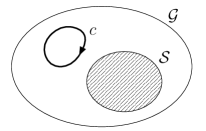
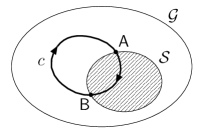
Figure 3: A closed loop $c$ running in ${\cal G}$.

(a)	(b)	(c)

The explicit form depends on how the loop $c$ runs in ${\cal G}$:

1. $c$ is contained in ${\cal S}$. (i.e. $c\subseteq{\cal S}$. ) See Fig. 3 (a).
   In this case ${\cal S}/(c\cap{\cal S})={\cal S}/c$ and ${\cal G}/(c\cup{\cal S})={\cal G}/{\cal S}$. Therefore

   $$[U_{{\cal G}/c}]_{\rm UV}^{\cal S}=U_{{\cal S}/c}\,U_{{\cal G}/{\cal S}}\quad\bigl{(}={\cal O}(\epsilon^{n_{\cal S}-1})\bigr{)}\,.$$ (62)

   The power of $\epsilon$ decreases by 1 since ${\cal S}/c$ has one less loops than ${\cal S}$.

2. $c$ runs outside of ${\cal S}$. (i.e.  $c\subseteq({\cal G}-{\cal S})$. ) See Fig. 3 (b).
   In this case ${\cal S}/(c\cap{\cal S})={\cal S}$ and ${\cal G}/(c\cup{\cal S})=({\cal G}/{\cal S})/c$. Therefore

   $$[U_{{\cal G}/c}]_{\rm UV}^{\cal S}=U_{\cal S}\,U_{({\cal G}/{\cal S})/c}\quad\bigl{(}={\cal O}(\epsilon^{n_{\cal S}})\bigr{)}\,.$$ (63)

3. $c$ is contained in both ${\cal S}$ and ${\cal G}-{\cal S}$. (i.e.  $c\cap{\cal S}\neq\emptyset$ and $c\cap({\cal G}-{\cal S})\neq\emptyset$. ) See Fig. 3 (c).
   In this case $c\cap{\cal S}$ is an open self-nonintersecting path within ${\cal S}$. It does not change the number of loops in ${\cal S}$ when the path is shrunken to a point. Therefore the scaling behavior is

   $$[U_{{\cal G}/c}]_{\rm UV}^{\cal S}={\cal O}(\epsilon^{n_{\cal S}})\,,$$ (64)

   though the exact factorization does not occur.

From these observations and Eq. (60) we find the following behavior of $B_{ij}$ in the UV limit.

1. $B_{ij}$ for $i,j\in{\cal S}$.
   The closed loops appearing in the sum in Eq. (60) fall into either of the cases (a) or (c), the former gives the leading contribution whereas the latter does not in the limit (55). Thus we have

   $$\left[B_{ij}\right]_{\rm UV}^{\cal S} =\sum_{c^{\prime}\subseteq{\cal S}}\ \xi_{i,c^{\prime}}\,\xi_{j,c^{\prime}}\,U_{{\cal S}/{c^{\prime}}}\,U_{{\cal G}/{\cal S}}$$ (65)

   $$=B_{ij}^{\cal S}\,U_{{\cal G}/{\cal S}}\,,$$

   where the superscript ${\cal S}$ denotes that $B_{ij}^{\cal S}$ is the $B$-function defined on the subdiagram ${\cal S}$.

2. $B_{ij}$ for $i,j\in{\cal G}/{\cal S}$.
   The closed loops appearing in the sum in (60) fall into either of the cases (b) or (c), both of which give the same order of contributions:

   $$\left[B_{ij}\right]_{\rm UV}^{\cal S}=\sum_{c^{\prime}\,\text{in case (\ref{case:cands:cinR})}}\,\xi_{i,c^{\prime}}\,\xi_{j,c^{\prime}}\,U_{{\cal G}/{c^{\prime}}}+\sum_{c^{\prime\prime}\,\text{in case (\ref{case:cands:cinboth})}}\,\xi_{i,c^{\prime\prime}}\,\xi_{j,c^{\prime\prime}}\,U_{{\cal G}/{c^{\prime\prime}}}\,.$$ (66)

   In the first term on the right-hand side the sum over closed loops $c^{\prime}\subseteq({\cal G}-{\cal S})$ is equivalent to the sum over loops in ${\cal G}/{\cal S}-\{s\}$, namely the loops in residual diagram ${\cal G}/{\cal S}$ that does not pass through the point $s$, where $s$ denotes a point into which the subdiagram ${\cal S}$ has shrunk. Therefore, the first term becomes

   $$U_{\cal S}\,\sum_{c^{\prime}\subseteq({\cal G}/{\cal S}-\{s\})}\,\xi_{i,c^{\prime}}\,\xi_{j,c^{\prime}}\,U_{({\cal G}/{\cal S})/{c^{\prime}}}\,.$$ (67)

   In the second term the closed loop $c^{\prime\prime}$ passing through the points $A,B\in{\cal S}\cap({\cal G}-{\cal S})$ is decomposed into two open paths ${\cal P}(AB)=c^{\prime\prime}\cap{\cal S}$ and ${\cal P}^{\prime}(AB)=c^{\prime\prime}\cap({\cal G}-{\cal S})$. The sum over $c^{\prime\prime}$ becomes the sum over a choice of points $A,B$ and open paths ${\cal P}(AB)$, ${\cal P}^{\prime}(AB)$. It is shown Nakanishi:1971 that $U_{{\cal S}/{\cal P}}$ satisfies

   $$U_{\cal S}=\sum_{{\cal P}(AB)}\,U_{{\cal S}/{\cal P}}\,.$$ (68)

   On the other hand the path ${\cal P}^{\prime}(AB)$ becomes a closed loop in ${\cal G}/{\cal S}$ that passes through the point $s$ to which $S$ has shrunk. Thus the second term becomes

   $$U_{\cal S}\,\sum_{c^{\prime\prime}\subseteq{\cal G}/{\cal S},\ c^{\prime\prime}\ni s}\,\xi_{i,c^{\prime\prime}}\,\xi_{j,c^{\prime\prime}}\,U_{({\cal G}/{\cal S})/{c^{\prime\prime}}}\,.$$ (69)

   From Eqs. (67) and (69) the UV-limit of $B_{ij}$ is

   $$\left[B_{ij}\right]_{\rm UV}^{\cal S}=B_{ij}^{{\cal G}/{\cal S}}\,U_{\cal S}\qquad i,j\in({\cal G}/{\cal S}).$$ (70)

3. $B_{mj}$ for $m\in{\cal S}$ and $j\in{\cal G}/{\cal S}$.
   This case is relevant only when ${\cal S}$ is a self-energy subdiagram, since for the vertex subdiagram case the leading contribution comes from the terms in which all lepton lines in ${\cal S}$ are contracted with each other.

   We denote the lines which are attached to the subdiagram ${\cal S}$ by $i$ and $i^{\prime}$. (See Fig. 4.)

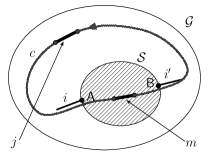
   Figure 4: A self-energy subdiagram $\cal S$ and a closed loop $c$ that passes through $m\in{\cal S}$ and $j\in{\cal G}/{\cal S}$.

   

   The closed loop $c$ that contains the lines $m\in{\cal S}$ and $j\in{\cal G}/{\cal S}$ passes through $i$ and $i^{\prime}$. The sum over loops $c$ is decomposed into the sum over ${\cal P}=c\cap{\cal G}$ and ${\cal P}^{\prime}=c\cap({\cal G}-{\cal S})$. It is shown Nakanishi:1971 that

   $$\sum_{{\cal P}}\,\xi_{m,{\cal P}}\,U_{{\cal S}/{\cal P}}=U_{\cal S}\,A_{m}^{\cal S}\,,$$ (71)

   where $A_{m}^{\cal S}$ is a scalar current on the line $m$ of the diagram ${\cal S}$. The path ${\cal P}^{\prime}$ turns into a closed path $c^{\prime}$ after shrinking ${\cal S}$ to a point which passes through the line $i\in{\cal G}/{\cal S}$. Therefore $B_{mj}$ becomes

   $$\left[B_{mj}\right]_{\rm UV}^{\cal S} =\left(\sum_{c^{\prime}}\,\xi_{j,c^{\prime}},\xi_{i,c^{\prime}}\,U_{({\cal G}/{\cal S})/{c^{\prime}}}\right)\,U_{\cal S}\,A_{m}^{\,\cal S}$$ (72)

   $$=B_{ij}^{{\cal G}/{\cal S}}\,A_{m}^{\,\cal S}\,U_{\cal S}\,.$$

The UV limit of the scalar current $A_{j}$ follows from Eq. (26) where the path ${\cal P}$ (which replaces $P^{\prime}$) is taken arbitrarily between two points attached to external lines. We can always choose the path to avoid the line $j$ so that $B^{\prime}_{ij}$ in Eq. (26) becomes $B_{ij}$.

When $\cal S$ is a vertex subdiagram, it is sufficient to consider only $A_{j}$ with $j\in{\cal G}/{\cal S}$, since in the leading contributions of the integrand all the lepton lines in $\cal S$ are contracted and there is no operator $D_{i}$ left to be turned into scalar current. The sum in Eq. (26) consists of two parts, one from ${\cal P}^{\prime}={\cal P}\cap{\cal S}$ and the other from ${\cal P}^{\prime\prime}={\cal P}\cap({\cal G}-{\cal S})$. In the limit (55) the scaling behavior (57) shows that the former part gives sub-leading contribution. Therefore, using Eq. (70), we obtain

$$\left[A_{j}\right]_{\rm UV}^{\cal S} =-\frac{1}{U_{{\cal G}/{\cal S}}}\sum_{i\in{{\cal G}/{\cal S}}}\eta_{i{\cal P}^{\prime\prime}}\,z_{i}\,B_{ij}^{\,{\cal G}/{\cal S}}$$ (73)

$$=A_{j}^{\,{\cal G}/{\cal S}}\,.$$

When ${\cal S}$ is a self-energy subdiagram, the scalar currents of both $j\in{\cal G}/{\cal S}$ and $j\in{\cal S}$ are relevant.

1. $A_{j}$ for $j\in{\cal G}/{\cal S}$.
   The same argument of the UV limit as in the vertex subdiagram applies to this case, which leads to

   $$\left[A_{j}\right]_{\rm UV}^{\cal S}=A_{j}^{\,{\cal G}/{\cal S}}\,.$$ (74)

2. $A_{m}$ for $m\in{\cal S}$.
   We choose the path ${\cal P}$ so that it avoids ${\cal S}$. Then all $B_{im}$ in (26) fall into the type III, whose UV limits are given by Eq. (72). Therefore,

   $$\left[A_{m}\right]_{\rm UV}^{\cal S} =-\frac{1}{U_{{\cal G}/{\cal S}}}\sum_{k\in{\cal P}}z_{k}\,B_{ik}^{\,{\cal G}/{\cal S}}A_{m}^{\,{\cal S}}$$ (75)

   $$=A_{i}^{\,{\cal G}/{\cal S}}\,A_{m}^{\,{\cal S}}\,,$$

   where $i$ is the line adjacent to $\cal S$.

We recall that $C_{ij}$ is derived from the part

$$-q^{\mu}\left[\frac{\partial\Lambda_{\mu}}{\partial q_{\nu}}\right]_{q=0}$$ (76)

of Eq. (36) with the external vertex inserted into the line $j$ and differentiated with respect to the external momentum $q_{\nu}$ flowing through the line $i$. When ${\cal S}$ is a vertex subdiagram, $C_{ij}$ for $i$ or $j$ in ${\cal S}$ have no overall UV divergence, since ${\cal S}$ has, effectively speaking, four legs: one photon line attached to the external vertex, the other internal photon line that is connected to ${\cal G}/{\cal S}$, and two internal lepton lines. So it is sufficient to consider the cases $i,j\in{\cal G}/{\cal S}$, in which the UV-limit of $C_{ij}$ becomes

$$\left[C_{ij}\right]_{\rm UV}^{\cal S}=\frac{1}{U_{{\cal G}/{\cal S}}}\,C_{ij}^{\,{\cal G}/{\cal S}}\,.$$ (77)

When ${\cal S}$ is a self-energy subdiagram, the definition (50) of $C_{ij}$ and the UV-limits of $B_{ij}$ lead to the following forms.

$$\left[C_{jk}\right]_{\rm UV}^{\cal S}=\frac{1}{U_{{\cal G}/{\cal S}}}\,C_{jk}^{\,{\cal G}/{\cal S}}\qquad j,k\in{\cal G}/{\cal S},$$ (78)

$$\left[C_{fg}\right]_{\rm UV}^{\cal S}=\frac{1}{U_{{\cal S}}}\,C_{fg}^{\,\cal S}+\frac{1}{U_{{\cal S}}}\left(A_{g}^{\,{\cal S}}\sum_{h\in{\cal S}}\,z_{h}B^{\prime\,{\cal S}}_{fh}-A_{f}^{\,{\cal S}}\sum_{h\in{\cal S}}\,z_{h}B^{\prime\,{\cal S}}_{gh}\right)\,\frac{1}{U_{{\cal G}/{\cal S}}}\sum_{j\in{\cal G}/{\cal S}}\,z_{j}B^{\prime\,{\cal G}/{\cal S}}_{ij},\qquad f,g\in{\cal S},$$ (79)

$$\left[C_{fj}\right]_{\rm UV}^{\cal S}=\frac{1}{U_{{\cal G}/{\cal S}}}\,A_{f}^{\cal S}\,C_{ij}^{\,{\cal G}/{\cal S}}+\frac{1}{U_{\cal S}}\sum_{g\in{\cal S}}\,z_{g}B^{\prime\,{\cal S}}_{fg}\,\frac{1}{U_{{\cal G}/{\cal S}}}\sum_{k\in{{\cal G}/{\cal S}}}\,z_{k}B^{\prime\,{{\cal G}/{\cal S}}}_{jk}\qquad f\in{\cal S},j\in{{\cal G}/{\cal S}},$$ (80)

where $i$ is the line adjacent to ${\cal S}$.

III.4 Factorization property of UV subtraction term

Now we proceed to examine the UV subtraction term along the steps of K-operation to see that it factorizes into two parts. For simplicity we consider a vertex part $\Gamma_{\cal G}^{\,\nu}$ defined in Eqs. (14) and (23), though the arguments apply to the general cases.

Suppose the UV divergent subdiagram $\cal S$ is a vertex subdiagram. In step (1) of K-operation we pick up the terms which are maximally contracted within ${\cal S}$. Such a term among the terms with $k$ contractions, $\dfrac{F_{k}}{U^{2+k}V^{n-k}}$, have the form:

$$\frac{1}{U^{2}V^{n-k}}\,\underbrace{\left\{\left(\frac{B_{ij}}{U}\right)\cdots\right\}}_{i,j\in{\cal S}}\,\underbrace{\left\{\left(\frac{B_{i^{\prime}j^{\prime}}}{U}\right)\cdots A_{l^{\prime}}\cdots\right\}}_{i^{\prime},j^{\prime},l^{\prime}\in{\cal G}/{\cal S}}\,.$$ (81)

The first factor in the braces is a product of $B_{ij}$’s with $i,j\in{\cal S}$, while the second factor is a product that consists of $(k-n_{\cal S})$ $B_{i^{\prime}j^{\prime}}$’s and several scalar currents whose indices $i^{\prime},j^{\prime}$ are in ${\cal G}/{\cal S}$.

In step (2) we consider the UV limit (55). It is achieved by replacing the building blocks $U$, $B_{ij}$ and $A_{j}$ by their UV limits, $[U]_{\rm UV}^{\cal S}$, $[B_{ij}]_{\rm UV}^{\cal S}$, and $[A_{j}]_{\rm UV}^{\cal S}$, respectively. Then Eq. (81) turns into

$$\underbrace{\frac{1}{U_{{\cal S}}^{\,2}}\left\{\left(\frac{B_{ij}^{\,{\cal S}}}{U_{\cal S}}\right)\cdots\,\right\}}_{\equiv g[{\cal S}]}\underbrace{\frac{1}{U_{{\cal G}/{\cal S}}^{\,2}}\left\{\left(\frac{B_{i^{\prime}j^{\prime}}^{\,{\cal G}/{\cal S}}}{U_{{\cal G}/{\cal S}}}\right)\cdots A_{l^{\prime}}^{\,{\cal G}/{\cal S}}\cdots\,\right\}}_{\equiv g[{\cal G}/{\cal S}]}\frac{1}{V_{{\cal G}/{\cal S}}^{\,n-k}}\,.$$ (82)

The first part depends only on $z_{i}$ with $i\in{\cal S}$, which we denote by $g[{\cal S}]$. The second part depends only on $z_{i}$ with $i\in{\cal G}/{\cal S}$. It is denoted similarly by $g[{\cal G}/{\cal S}]$. In the naïve UV limit $V$ leads to $V_{{\cal G}/{\cal S}}$.

In step (3) $V_{{\cal G}/{\cal S}}$ is replaced by $V_{\cal S}+V_{{\cal G}/{\cal S}}$. The integral now becomes

$$\int(dz)_{\cal G}\,g[{\cal S}]\,g[{\cal G}/{\cal S}]\,\frac{1}{\left(V_{\cal S}+V_{{\cal G}/{\cal S}}\right)^{n-k}}\,.$$ (83)

We shall see that it factorizes into $\cal S$ and ${\cal G}/{\cal S}$ parts. Firstly, the identity

$$1=\int_{0}^{1}\frac{ds}{s}\,\delta\left(1-\frac{z_{\cal S}}{s}\right)\ \int_{0}^{1}\frac{dt}{t}\,\delta\left(1-\frac{z_{{\cal G}/{\cal S}}}{t}\right)\,,$$ (84)

is inserted into the integral, where $z_{\cal S}$ and $z_{{\cal G}/{\cal S}}$ are defined by $\displaystyle z_{\cal S}=\sum_{i\in{\cal S}}z_{i}$ and $\displaystyle z_{{\cal G}/{\cal S}}=\sum_{i\in{\cal G}/{\cal S}}z_{i}$, respectively. Secondly, we rescale the Feynman parameters as follows:

$$z_{i}\to sz_{i} \qquad i\in{\cal S}$$ (85)

$$z_{i}\to tz_{i} \qquad i\in{{\cal G}/{\cal S}}$$

Since $V$-functions are homogeneous polynomial of degree 1, they scale in such a manner as $V_{\cal S}\to s\,V_{\cal S}$ and $V_{{\cal G}/{\cal S}}\to t\,V_{{\cal G}/{\cal S}}$. Other parts of the integrand and the integration measure also scale accordingly.

Then using the Feynman integral formula:

$$\Gamma(k+l)\int_{0}^{1}ds\,dt\ \delta(1\!-\!s\!-\!t)\,\frac{s^{k-1}t^{l-1}}{(sA+tB)^{k+l}}=\frac{\Gamma(k)}{A^{k}}\,\frac{\Gamma(l)}{B^{l}}\,,$$ (86)

the integral is shown to be factorized into two parts:

$$\int dz_{\cal S}\,\delta(1\!-\!z_{\cal S})\,g[{\cal S}]\int dz_{{\cal G}/{\cal S}}\,\delta(1\!-\!z_{{\cal G}/{\cal S}})\,g[{\cal G}/{\cal S}]\int ds\,dt\,\delta(1\!-\!s\!-\!t)\,\frac{s^{\alpha-1}t^{\beta-1}}{\left(sV_{\cal S}+tV_{{\cal G}/{\cal S}}\right)^{\alpha+\beta}}$$ (87)

$$\qquad=\int(dz)_{\cal S}\,\frac{g[{\cal S}]}{V_{\cal S}^{\ \alpha}}\times\int(dz)_{{\cal G}/{\cal S}}\,\frac{g[{\cal G}/{\cal S}]}{V_{{\cal G}/{\cal S}}^{\ \beta}}\,,$$

where $\alpha$ and $\beta$ are constants determined by the rescaling (85).

Based on those observations the whole integral of the vertex part $\Gamma_{\cal G}^{\nu}$ is shown to be factorized in UV limit as

$${\sf K}_{\cal S}\Gamma_{\cal G}^{\ \nu}=L^{\rm UV}_{\cal S}\Gamma_{{\cal G}/{\cal S}}^{\ \nu}\,,$$ (88)

where $L^{\rm UV}_{\cal S}$ is the UV divergent part of the vertex renormalization constant $L_{\cal S}$ and $\Gamma_{{\cal G}/{\cal S}}^{\ \nu}$ is the vertex part of the residual diagram ${{\cal G}/{\cal S}}$.

When $\cal S$ is a self-energy subdiagram, the factorization is not apparent because not all ${\hskip 1.99997pt/\hskip-7.5pt{}D}{}_{m}$ with $m\in{\cal S}$ are contracted. From Eqs. (72) and (75) we can symbolically write the uncontracted ${\hskip 1.99997pt/\hskip-7.5pt{}D}{}_{m}$ as

$$\left[{\hskip 1.99997pt/\hskip-7.5pt{}D}{}_{m}\right]_{\rm UV}^{\cal S}=A_{m}^{\,{\cal S}}\,{\hskip 1.99997pt/\hskip-7.5pt{}D}{}_{i^{\prime\prime}}^{\,{{\cal G}/{\cal S}}}\,,$$ (89)

where $i^{\prime\prime}$ is a fictitious line related to $i$ and $i^{\prime}$. After a little algebra one finds Cvitanovic:1974um ; Kinoshita_book

$${\sf K}_{\cal S}\Gamma_{\cal G}^{\ \nu}={\delta m}^{\rm UV}_{\cal S}\Gamma_{{\cal G}/{\cal S}(i^{*})}^{\ \nu}+B^{\rm UV}_{\cal S}\Gamma_{{\cal G}/{\cal S},i^{\prime}}^{\ \nu}\,,$$ (90)

where ${\delta m}^{\rm UV}_{\cal S}$ is the UV divergent part of the mass renormalization constant $\delta m_{\cal S}$ and $B^{\rm UV}_{\cal S}$ is that of the wave function renormalization constant $B_{\cal S}$. ${\cal G}/{\cal S}(i^{*})$ denotes the diagram obtained by shrinking ${\cal S}$ to a point, where $i^{*}$ indicates two-point vertex between lines $i$ and $i^{\prime}$. ${\cal G}/{\cal S},i^{\prime}$ denotes the diagram derived from ${\cal G}$ by shrinking ${\cal S}$ to a point and eliminating the line $i^{\prime}$. It can be reduced to the form $\Gamma_{{\cal G}/{\cal S}}^{\ \nu}$ after integration by part with respect to $z_{i}$.

The factorization of K-operation is crucial when there are more than one subdiagrams that cause UV divergences, since this property guarantees that the successive operation of ${\sf K}_{{\cal S}_{k}}$ is consistent with the forest structure.

IV Forest formula

A Feynman diagram that appears at higher-order terms of perturbation theory may have complicated UV-divergence structures. In many textbooks they are treated in a recursive formulation so that the inner subdivergences of a renormalization part should be subtracted prior to the subtraction of its own overall divergence. It is natural in the framework of renormalization theory, for it is derived from the requirement that the divergences should be resolved by local counterterms. It is also tractable in general for hand manipulations since the subtractions are performed step by step from lower order parts and the number of steps are, as it turns out, relatively small. It is, however, not so convenient in our numerical approach in which the singularities due to the UV divergences are canceled point-by-point in the Feynman parameter space. To achieve this we have to prepare the subtraction terms as integrals defined in the same parameter space as that of the original unrenormalized amplitude.

An explicit solution of the recursive formulation is given by Zimmermann’s forest formula Zimmermann:1969jj . Each source of the UV-divergence is related to a forest, a set of UV-divergent subdiagrams, and the subtraction term associated with the forest is constructed by the subtraction operations for the subdiagrams applied successively to the unrenormalized amplitude. The whole subtraction terms are generated along the complete set of forests.

In our numerical approach the subtraction operation is given by K-operation for a single subdivergence. As seen in the previous section it retains the factorization property, which guarantees the successive K-operations. Therefore, once a UV-divergent structure is known in the form of a forest, we can obtain the integrand of the subtraction term Cvitanovic:1974um . Although the subtraction scheme presented here is identical with that developed in Ref. Cvitanovic:1974um , it is more readily adaptable for code generation.

The forest formula is much more useful for the automated scheme. The forests are given by the combinations of non-overlapping subdiagrams. So the complete identification of UV-divergent structures is obtained by purely combinatorial procedure from the set of all UV-divergent subdiagrams. Thus it is readily implemented in terms of forests, which enables us to obtain fully UV-renormalized amplitude of a diagram $\cal G$.

IV.1 Definition of forests

We begin with the inclusion relations between subdiagrams. When two subdiagrams ${\cal S}_{i}$ and ${\cal S}_{j}$ share no vertices nor lines they are called disjoint. When all lines of ${\cal S}_{i}$ belong to ${\cal S}_{j}$, the subdiagram ${\cal S}_{i}$ is included in the subdiagram ${\cal S}_{j}$. In this case ${\cal S}_{i}$ and ${\cal S}_{j}$ are called nested. Otherwise they are called overlapping, in which ${\cal S}_{i}$ and ${\cal S}_{j}$ share some vertices and lines while one is not included in the other.

A forest is defined as a set of subdiagrams whose elements satisfy the condition that any pairs of them are disjoint or nested. (The empty set is also allowed.) When a forest contains the diagram $\cal G$ itself, it is called full forest. Otherwise it is normal forest. For the calculation of $g\!-\!2$ term it is sufficient to consider only normal forests. We denote the set of all possible normal forests of a diagram $\cal G$ by $\mathfrak{F}({\cal G})$.

IV.2 Forest formula and K-operations

Assume $\mathfrak{C}_{\cal S}$ is a subtraction operator associated with a subdiagram $\cal S$. The renormalized amplitude $M^{\prime}_{\cal G}$ of a diagram $\cal G$ is obtained from the unrenormalized amplitude $M_{\cal G}$ by forest formula Zimmermann:1969jj :

$$M^{\prime}_{\cal G}=\sum_{f\in\mathfrak{F}({\cal G})}\left[\prod_{{\cal S}_{i}\in f}(-\mathfrak{C}_{{\cal S}_{i}})\right]M_{\cal G}\,.$$ (91)

Here the sum is taken over all forests $f$ of the diagram $\cal G$. The order of operation in the product is arranged so that the inner subdiagrams are applied first.

In our approach the subtraction operation is provided as K-operation for performing the intermediate renormalization in numerical procedure. Recall that the integrand of the subtraction term obtained by K-operation factorizes exactly into the UV-divergent part of renormalization constant and the lower-order $g\!-\!2$ term by construction. This feature enables us to apply repeatedly K-operations if there is another UV-divergent subdiagram in the forest.

IV.3 Procedure

The subtraction term associated with a forest is obtained by the successive K-operations. The concrete procedure is given as follows. Suppose the forest $f$ consists of $m$ subdiagrams, $f=\{{\cal S}_{1},\dots,{\cal S}_{m}\}$. They are arranged in such an order that the inner subdiagrams come ahead.

The scaling like Eq. (55) for a forest $f$ can be defined similarly by introducing the scaling parameters $\left\{\epsilon_{k}\right\}_{k=1,\,\cdots,\,m}$ as

$$z_{i}=O(\epsilon_{k})\qquad i\in{\cal S}_{k},$$ (92)

where ${\cal S}_{k}$ is the inner-most subdiagram of the forest $f$ which contains the line $i$. We define the UV limit $\left[g(\{z_{j}\})\right]^{f}_{\rm UV}$ of a function $g(\{z_{j}\})$ of Feynman parameters as the leading term of $g(\{z_{j}\})$ in the successive limits

$$\left[g(\{z_{j}\})\right]^{f}_{\rm UV}=\lim_{\epsilon_{m}\rightarrow 0}\cdots\lim_{\epsilon_{1}\rightarrow 0}g(\{z_{j}\})\,.$$ (93)

Due to the factorization property we can construct the subtraction term corresponding to the forest $f$ by the repeated applications of K-operations. The K-operation for $k$th subdiagram ${\cal S}_{k}$ is applied to the reduced diagram ${\cal G}/({\cal S}_{1}\cup\cdots\cup{\cal S}_{k\!-\!1})$ which has been obtained by shrinking the subdiagrams up to $(k-1)$th subdiagrams to points. The integrand of the subtraction term is obtained in the following way.

1. In Eq. (53) collect all terms which are maximally contracted within the subdiagram ${\cal S}_{i}$ for $i=1,\dots,m$.

2. Replace $U$, $B_{ij}$, $C_{ij}$ and $A_{j}$ appearing in the integrand by their UV limits, $\left[U\right]_{\rm UV}^{f}$, $\left[B_{ij}\right]_{\rm UV}^{f}$, $\left[C_{ij}\right]_{\rm UV}^{f}$, and $\left[A_{j}\right]_{\rm UV}^{f}$, respectively.

3. Arrange $V$ in the limit to take the form

   $$V_{\widetilde{{\cal S}_{1}}}+\cdots+V_{\widetilde{{\cal S}_{m}}}+V_{{\cal G}/({\cal S}_{1}\cup\cdots\cup{\cal S}_{m})}\,,$$ (94)

   where $\widetilde{{\cal S}_{k}}$ is a subdiagram obtained from ${\cal S}_{k}$ by shrinking all inner subdiagrams to points.

4. Attach the overall sign $(-1)^{m}$.

The end result of this construction is identical with what was obtained in Refs. kl1 ; Cvitanovic:1974um ; Kinoshita_book . The advantage of the forest approach is that it is readily translatable into computer code, which of course is crucial for automation of our entire formulation.

V q-Type Feynman diagrams

In this section and the next we focus on the particular type of diagrams which have no closed lepton loops. We call such a diagram as q-type. The q-type diagram has a simple structure, which allows simple identification of various graph-theoretical notions embedded in the diagram. The key features relevant for automated scheme of calculations may be listed as follows:

1. systematic generation of diagrams are easily done.

2. a set of independent loops are easily identified.

3. subdiagrams relevant for the UV divergence are easily identified.

They enable us to develop efficient algorithms and implementations.

In this section the features (a) and (b) are discussed. A set of algorithms to obtain the complete set of topologically independent diagrams is presented. The feature (b) is related to the construction of the topological forms $B_{ij}$ and $U$, which provide the building blocks of the integrand. The feature (c) will be discussed in the next section in relation to the subtraction of UV divergences.

V.1 Definition and diagram representation

A q-type self-energy-like diagram of $2n$th order is given by a path ${\cal P}$ consisting of lepton lines emanating from the incoming lepton $\bar{\psi}(y)$ and terminating at the outgoing lepton $\psi(x)$, with $n$ photon lines attached to the path at their both ends; there is no closed lepton loop. A typical diagram is shown in Fig. 5. In QED there is only one type of interaction, the coupling of electromagnetic current $j^{\mu}=\bar{\psi}\gamma^{\mu}\psi$ to the gauge potential $A_{\mu}$, which is represented in Feynman rules as a trivalent vertex, at which a photon line is attached to the lepton line path. Here we consider only one-particle irreducible (1PI) diagrams.

We denote $2n$ vertices as $v_{j}$ $(j=0,\dots,(2n-1))$, and adopt the following convention throughout the rest of the paper. Every q-type diagram is drawn in such a way that the path ${\cal P}$ passes from the right to the left. The vertices $v_{j}$ sequentially lie on the path ${\cal P}$ as $v_{0}\,\dots,v_{2n-1}$ from the left to the right. A lepton line is denoted as $l_{k}$ $(k=1,\dots,(2n-1))$ which runs from a vertex $v_{k}$ to another vertex $v_{k-1}$. A photon line which connects two vertices $v_{i_{k}}$ and $v_{j_{k}}$, is denoted as $h_{k}$ $(k=a,b,\dots)$, where label $k$ is taken to be an alphabet. The photon line is also represented by the pair of two endpoints $(v_{i_{k}},v_{j_{k}})$. For later convenience, a direction of the photon line is chosen by $v_{i_{k}}\rightarrow v_{j_{k}}$ where the indices are ordered as $i_{k}<j_{k}$. We also denote the lines collectively as $\{l\}$.

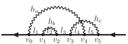
Figure 5: An example of q-type diagram.

A q-type diagram ${\cal G}$ is uniquely specified by the set of $n$ photon lines, i.e., the set of pairs of vertices as

$${\cal G}=\left\{(v_{i_{1}},v_{j_{1}}),\dots,(v_{i_{n}},v_{j_{n}})\right\}\,,$$ (95)

where $i_{1},j_{1},\dots,i_{n},j_{n}$ take values in $\{0,\dots,(2n-1)\}$ exclusively. To avoid the ambiguity of representation, we further impose the following condition:

$$i_{k}<j_{k}, \quad\text{for each pair}\ (v_{i_{k}},v_{j_{k}}),$$ (96)

$$i_{k}<i_{k^{\prime}}, \quad\text{between two pairs}\ k<k^{\prime}\,.$$

V.2 Circuits and loop matrix

Consider the chain diagram associated with a q-type diagram. A circuit of the graph is a self-nonintersecting closed path along the graph. The maximal independent set of them defines a fundamental set of circuits, which provides a complete basis of closed loops of the graph. The fundamental set of circuits of a graph is crucial in the calculation of $U$ and $B_{ij}$.

In the case of q-type diagram, a path ${\cal C}_{r}$ composed of a photon line $h_{r}=(v_{i_{r}},v_{j_{r}})$ and lepton lines $l_{i_{r}+1},\dots,l_{j_{r}}$ that lie between two endpoints of the photon line form a circuit. The direction of the circuit can be taken naturally along those of lepton and photon lines. The fundamental set is thus chosen by the set of paths $\left\{{\cal C}_{r}\right\}_{r=1,\dots,n}$.

The loop matrix $\xi_{j,{\cal C}_{r}}$ is given almost trivially. Once $\xi_{j,{\cal C}_{r}}$ is known, $U$ and $B_{ij}$ are calculated according to the formula (29), (30), and (31) given in Section II, or (109), (110), and (112) in Appendix B.

V.3 Time-reversal symmetry

By using the time-reversal symmetry of QED, we can further relate distinct diagrams to each other, to reduce independent set of diagrams. Two q-type Feynman diagrams are equivalent in time-reversal and give rise to the same contribution to anomalous magnetic moment if and only if they are the images of each other under the reversal of the directions of all lepton lines in ${\cal P}$.

For a time-reversal equivalent pair of diagrams, it is sufficient to evaluate either of the two. The asymmetric diagrams in time-reversal dominate at higher orders, which implies that the number of distinct diagrams to be evaluated is cut down to almost half by considering time-reversal symmetry.

V.4 Algorithms

Suppose $2n$ vertices are placed on a lepton line path ${\cal P}$. Then the complete set of topologically distinct q-type diagrams of $2n$th order is obtained as follows:

• Connect a pair of vertices by a photon line in every possible way.

• Pick only 1PI diagrams and discard others.

• Drop either of the pair of equivalent diagrams under time-reversal.

Step 1 is a process to list up all possible ways to make $n$ pairs out of the vertices $\{0,\dots,(2n-1)\}$. A procedure to make $k$ pairs from $2k$ elements is given as follows; the elements are assumed to be ordered in a line.

Pick an element at the left end of the line, and another one from the rest to form a pair. Repeat the process to the remaining $2k-2$ elements to make $k-1$ pairs until there is no element left.

By considering $2k-1$ ways to make a pair, we can generate all possible pairings recursively. The total number of ways is $(2k-1)!!$.

Next we go to step 2. The diagram corresponding to a pairing generated above may not satisfy the 1PI condition. Since a q-type diagram is connected by lepton lines, it is sufficient to check whether it stays connected when one of the lepton lines is eliminated.

A q-type diagram is 1PI if and only if for each lepton line $l_{k}$, there exists at least one photon line that steps over the lepton line, i.e., two end points of photon line, $(v_{i},v_{j})$, satisfy $v_{i}\leq v_{k-1}$ and $v_{j}\geq v_{k}$ simultaneously.

The diagrams that do not match the condition shall be discarded.

The time-reversal operation in step 3 is done by substituting the index $k$ of vertex $v_{k}$ by $2n-1-k$. A q-type diagram ${\cal G}$ is mapped to ${\cal G}^{\prime}$ by the substitution of indices followed by the reshuffling of pairs to satisfy the conventions (96). If ${\cal G}$ is invariant under the time-reversal, it should be kept with the symmetry factor one. Otherwise, either of ${\cal G}$ or ${\cal G}^{\prime}$ should be kept with the symmetry factor two; we adopt the rule that the diagram ${\cal G}$ is chosen when the lexicographical order of the patterns of indices representing the diagrams ${\cal G}$ is ahead of ${\cal G}^{\prime}$.

V.5 Number of diagrams

Based on the above consideration, the number of 1PI q-type diagrams ${\cal N}_{n}$ of $n$ loops is given recursively by the following relation (disregarding time-reversal symmetry):

$${\cal N}_{n}=(2n-1)!!-\sum_{(k_{1},\dots,k_{m})\in{\mathfrak{P}}_{n}}\prod_{j}\,{\cal N}_{k_{j}}\,,$$ (97)

where ${\mathfrak{P}}_{n}$ denotes the set of ordered partitions of $n$ (i.e. $(1,2)$ and $(2,1)$ should be distinguished).

Table 1 shows the number $N_{n}$ of independent q-type diagrams for $n\leq 7$ as well as that of symmetric ones and that of asymmetric ones under time-reversal. (${\cal N}_{n}=N_{n}^{\phantom{n}\text{sym}}+2N_{n}^{\phantom{n}\text{asym}}$.)

Table 1: The number of independent 1PI diagrams of q-type, $N_{n}$, with $n$ loops.

$n$	$N_{n}$	$N_{n}^{\phantom{n}\text{sym}}$	$N_{n}^{\phantom{n}\text{asym}}$
1	1	1	0
2	2	2	0
3	8	6	2
4	47	20	27
5	389	72	317
6	4226	290	3936
7	55804	1198	54606

It also demonstrates that the incorporation of time-reversal symmetry efficiently reduces the number of independent diagrams to be evaluated $\left(N_{n}^{\phantom{n}\text{sym}}+N_{n}^{\phantom{n}\text{asym}}\right)$ at higher orders.

VI UV divergence structure of q-type diagrams

For a given Feynman diagram, it is required in the renormalization process to pick up all the 1PI subdiagrams that have overall ultraviolet (UV) divergence. They are referred to as UV divergent 1PI subdiagrams. By the power counting of superficial divergence, there are two types of UV divergent subdiagrams in q-type diagrams in QED, namely, the lepton self-energy-like subdiagram, and the vertex subdiagram. Every subtraction term in the subtractive renormalization procedure corresponds to the Zimmermann’s forest, a combination of subdiagrams whose loop momenta go to infinity.

For a q-type diagrams, the above prescription is implemented quit simply, reflecting the graph theoretical properties of the diagram. In this section we discuss the UV structure of the q-type diagrams and describe an algorithm to compose subdiagrams and forests of the diagram.

VI.1 UV divergent subdiagrams

A subdiagram relevant for the UV divergence is either of the self-energy type or of the vertex type. For a q-type diagram in which all vertices are located on the lepton line path $\cal P$ a subset of vertices are denoted by one or more segments of the path. Thus a subdiagram of these types of a q-type diagram corresponds to a single segment of the path, and it is specified by the indices of two end-point vertices.

Therefore, to obtain all the divergent subdiagrams of a q-type diagram we have only to find every possible pair of indices $[i,j]$, $0\leq i<j\leq(2n-1)$ that satisfies the following two conditions:

The subdiagram corresponding to the segment $[i,j]$ is classified into the self-energy-like type or the vertex type. The number of ‘floating’ photon line (only either one of the two endpoints of the photon line lies on the segment $[i,j]$) is zero (for self-energy-like subdiagram) or one (for vertex subdiagram).

And,

It is one-particle irreducible, i.e., it stays connected when any one of the lepton lines that belong to the subdiagram is eliminated.

The second condition is satisfied when for every lepton line, $l_{i+1},\dots,l_{j}$, there is at least one photon line that belongs to the subdiagram (both endpoints of it lie between $v_{i}$ and $v_{j}$) which steps over the lepton line. The photon line $h_{k}=(v_{i_{k}},v_{j_{k}})$ steps over the lepton line $l_{s}=(v_{s-1},v_{s})$ when $i\leq i_{k}\leq s-1$ and $s\leq j_{k}\leq j$ simultaneously.

It is noted that subdiagrams of q-type diagrams also do not contain lepton loops. The residual diagram of a q-type diagram which is obtained by shrinking the subdiagram to a point is again of q-type. Recall that it is related to lower-order $g-2$ term. The UV subtraction procedure is closed within the q-type diagrams.

VI.2 Forests

To begin with, we define the inclusion relation between two subdiagrams, $S_{a}$ and $S_{b}$:

disjoint

if $S_{a}$ and $S_{b}$ do not share any vertices nor lines, i.e. $S_{a}\cap S_{b}=\emptyset$.

overlapping

if $S_{a}$ and $S_{b}$ share some vertices and lines though one is not completely included in the other.

nested

if $S_{a}$ (or $S_{b}$) is a subset of the other, i.e. $S_{a}\subset S_{b}$ or $S_{a}\supset S_{b}$.

For the q-type diagrams, the inclusion relation is mapped to that of two segments. The relation between two subdiagrams represented by $S_{a}=[i_{a},j_{a}]$ and $S_{b}=[i_{b},j_{b}]$ is one of the following (assuming that $i_{a}\leq i_{b}$):

disjoint  if $j_{a}<i_{b}$,
overlapping  if $i_{a}<i_{b}\leq j_{a}<j_{b}$,
nested  if $i_{a}\leq i_{b}$ and $j_{b}\leq j_{a}$.

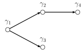
Figure 6: A forest composed of nested subdiagrams $\gamma_{1},\dots,\gamma_{4}$ (left), and the corresponding cascade structure (right).

A forest is defined as such a set of subdiagrams that any two of its elements are not overlapping with each other; they are disjoint or nested. Since we are currently interested in the magnetic form factor, it is sufficient to consider only the ‘normal’ forests which do not contain the diagram $\cal G$ itself. On the other hand, a forest that contains $\cal G$ is called ‘full’ forest.

A complete set of forests of a diagram is generated by finding all the combinations of the subdiagrams, and discarding those which contain the overlapping subdiagrams. (This particular procedure is not restricted to the q-type diagrams.) A cascade structure of subdiagrams of a forest is reproduced by referring to the inclusion relation between subdiagrams. This information is required during the subtraction process which is performed for the divergence corresponding to the inner subdiagrams first.

VII Automated flow of calculation

In this section we present the flow of the process to generate the numerical integration code for evaluating an individual diagram from its representation indicated by the rectangular box at the upper-left corner of Fig. 7.

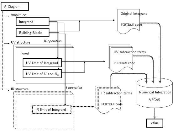
Figure 7: Flow of process to generate the numerical integration codes from the diagram representation.

The provided information enables us to construct the amplitude in the form of Feynman parametric integrals in terms of building blocks, $U$, $B_{ij}$, scalar currents, and so forth. This follows exactly the pattern developed for the sixth- and eighth-order cases Cvitanovic:1974uf ; kl1 . Next, the ultraviolet divergence is treated via K-operation which identifies and subtracts the most divergent part of the original integral, corresponding to a specific UV limit. The treatment of the whole divergence structure is organized by the Zimmermann’s forest formula. The infrared divergence remaining in the individual diagram should also be subtracted away, though this article does not cover this subject. Finally, the (intermediate-) renormalized amplitude constructed from the original amplitude and the set of subtraction terms is turned into a FORTRAN code, which is readily processed by the numerical integration system such as VEGAS lepage , an adaptive Monte-Carlo integration routine.

VII.1 Diagram generation

We begin by generating a complete set of topologically distinct q-type diagrams of a given order according to the algorithm in Section V.4. The implementation of the algorithm is achieved in C++. Each diagram is expressed by a single-line representation which describes the pattern of pairings of vertices by the photon propagators. The diagrams are then named after a certain convention and stored in a plain text file. All subsequent steps refer to this file for the diagram data.

Names and forms of all relevant diagrams of the sixth- and the eighth-orders are listed in Refs. kn2 ; Kinoshita_book . We adopt the following convention for the tenth-order diagrams. The W-T summed diagrams are classified into two groups, one of which is time-reversal symmetric (72 diagrams) and the other is asymmetric (317 diagrams). They are sorted in a lexicographical order within each group, and then given serial numbers with a prefix “X” which stands for the tenth-order in a Roman numeral, first for the symmetric ones (X001, …, X072), then for the asymmetric ones (X073, …, X389).

VII.2 Subdiagram search and forest construction

All UV divergent subdiagrams of a q-type diagram are identified according to the algorithms in Section VI.1. Then all forests are constructed according to the description in Section VI.2 by generating every possible combination of subdiagrams which does not contain any overlapping pairs. The inclusion relation between subdiagrams is examined prior to this step.

The cascade structure among the subdiagrams of a forest is also identified and stored in a tree form. It is, however, not mandatory since the order of successive subtraction operations of a forest is automatically respected if we adopt the regulation that the diagrams of smaller sizes are processed first. It is because the sizes of subdiagrams $S_{i}$ and $S_{j}$ satisfy $S_{i}<S_{j}$ whenever $S_{i}$ is contained in $S_{j}$.

The implementation is carried out in both Perl and C++. To demonstrate the fast algorithms and implementations we generated the diagrams and their forests up to 14th order, which took less than 10 minutes on an ordinary PC.

VII.3 Constructing unrenormalized integrand

A single-line representation of a q-type diagram may be directly translated into the form of unrenormalized integrand. Recall that the integrand $\mathbb{F}$ of a q-type diagram is given by Eq. (44):

$$\mathbb{F}=\gamma^{\mu_{1}}\left({\hskip 1.99997pt/\hskip-7.5pt{}D}{}_{1}+m_{1}\right)\gamma^{\mu_{2}}\cdots\gamma^{\mu_{2n\!-\!1}}\left({\hskip 1.99997pt/\hskip-7.5pt{}D}{}_{2n\!-\!1}+m_{2n\!-\!1}\right)\gamma^{\mu_{2n}}\,\times\prod_{k=1}^{n}\,g_{\mu_{i_{k}}\mu_{j_{k}}}\,,$$ (98)

where the diagram-specific product $\prod g_{\mu_{i_{k}}\mu_{j_{k}}}$ in this case is determined by the pairing pattern

$$\left\{(v_{i_{1}},v_{j_{1}}),\,(v_{i_{2}},v_{j_{2}}),\dots\right\}\,.$$ (99)

The basic form of integrand is common to all q-type diagrams, where we have only to make permutation of indices to construct the integrand of a particular diagram. Therefore we can make full use of a template to perform this step.

We implemented this step as a Perl program, which translates the single-line representation of the diagram into an explicit form of $\mathbb{F}$ and put it into a template of FORM program. It is then processed by FORM to perform the analytic integration over all loop momenta, the trace calculation, contractions of $D$ operators, and other algebraic manipulations, which yields the unrenormalized integrand expressed as a polynomial of the building blocks, $U$, $B_{ij}$, $C_{ij}$ and $A_{j}$, integrated over Feynman parameters. This follows exactly the method developed for the sixth- and eighth-order cases Cvitanovic:1974uf ; kl1 . The output is in the FORM-readable form for the subsequent steps of deriving various UV limits, as well as in the form of FORTRAN code.

VII.4 Constructing building blocks

The building blocks of integrand, $U$ and $B_{ij}$, are determined from the underlying topological structure of the diagram called chain diagram Cvitanovic:1974uf ; Kinoshita_book . First we identify chains and chain variables $z_{\alpha}=\sum_{i\in\alpha}z_{i}$. The fundamental set of circuits $\{{\cal C}_{r}\}_{r=1,\dots,n}$ of the diagram is identified according to the specification in Section V.2, and the loop matrix $\xi_{\alpha,{\cal C}_{r}}$ is constructed accordingly. Once $\xi_{\alpha,{\cal C}_{r}}$ is known the building blocks $U$, $B_{ij}$ are obtained as homogeneous polynomials of $\{z_{\alpha}\}$ by Eqs. (29), (30), and (31). Other building blocks, $\widetilde{C}_{ij}$ $(C_{ij}=\widetilde{C}_{ij}/U)$, $A_{j}$, and $V$ are also constructed in terms of $U$, $B_{ij}$ and Feynman parameters $\{z_{i}\}$ by Eqs. (50), (26), (16), and (52):

$$A_{j}=\frac{1}{U}\sum_{i}z_{i}\,B^{\prime}_{ij}\,,$$ (100)

$$V=\sum_{i}z_{i}-G\,,\qquad G=\sum_{i}z_{i}\,A_{i}\,,$$ (101)

where the sum runs over all lepton lines.

The calculation of $U$, $B_{ij}$ and $\widetilde{C}_{ij}$ involves algebraic manipulations such as determinants and cofactors of matrices whose elements are polynomials of Feynman parameters $\{z_{\alpha}\}$. We implemented this step in three ways.

1. The algebraic manipulations are performed by MAPLE. We identify the loop matrix from the diagram representation and prepare a MAPLE program to calculate $U$, $B_{ij}$, and $C_{ij}$ according to Eqs. (29), (30), (31), and (50). The output is in the FORM-readable form for the subsequent operations. The FORTRAN code is also generated from it via FORM.

2. We developed concise formulae, (109) and (110), to provide the coefficients of the $U$-function directly from the loop matrix. The coefficients $u_{p_{1}p_{2}\dots p_{m}}$ are defined by

   $$U=\sum_{\{p_{i}\}}\,u_{p_{1}p_{2}\dots p_{m}}\,z_{\alpha_{1}}^{\,p_{1}}\,z_{\alpha_{1}}^{\,p_{1}}\dots z_{\alpha_{n}}^{\,p_{m}}\,,$$ (102)

   for every possible combination of $\{p_{i}\}$, where $p_{i}$ takes $0$ or $1$ and $\displaystyle\sum_{i=1}^{m}p_{i}=n$. $m$ is the total number of chains. Similarly for $B_{ij}$ and $C_{ij}$ by the formulae described in Appendix B. They are implemented in C++.

3. The algebraic manipulations are also handled in C++ by constructing proper data structures (or classes). We developed a simple polynomial class and implemented the calculation of $U$ and $B_{ij}$ according to Eqs. (29), (30), and (31). We also developed another version with the help of GiNaC ginac , an algebraic manipulation library in C++.

The current version of automation system relies on the implementation i) for no particular reason. The scalar currents $A_{j}$ and the function $V$ are constructed from $U$ and $B_{ij}$ according to Eqs. (100) and (101).

VII.5 Constructing UV subtraction terms

The UV divergences of a diagram are identified as Zimmermann’s forests which are the combinations of UV divergent subdiagrams. We construct a set of UV subtraction terms, each of which corresponds to a particular forest, by the successive applications of K-operations to the unrenormalized integrand.

The subtraction term is constructed by the following three steps.

1. Find the UV limit of the building blocks.

2. Find the UV limit of the integrand.

3. Modify the UV limit of $V$-function in the denominator to satisfy the factorizability requirement of subtraction terms.

Those steps are achieved by simple power counting applied to the original (unrenormalized) integrand and building blocks, without referring to any lower-order constructs. The whole implementation is done in Perl with the help of MAPLE and FORM for symbolic manipulations. This follows exactly the scheme developed for the sixth- and eighth-order cases Cvitanovic:1974uf ; kl1 .

VII.5.1 UV limit of building blocks

The explicit form of building blocks, $U$, $B_{ij}$, and $\widetilde{C}_{ij}$, in the UV limit (55) related to a subdiagram ${\cal S}$ is given as the leading term in power series expansion by $\epsilon$ under the rescaling of the Feynman parameters as

$$z_{i}\to\epsilon\,z_{i}\,,\qquad i\in{\cal S}\,.$$ (103)

The procedure is implemented as a MAPLE or FORM program, in which the scaling rules (103) are generated from the information of the subdiagram.

For a forest consisting of more than one subdiagrams the above procedure is successively applied with each subdiagram ${\cal S}_{k}$. The order of operations is determined referring to the cascade structure of the forest so that the inner subdiagrams are applied first.

The UV limit of scalar current $A_{j}$ is constructed from the UV limits of $U$ and $B_{ij}$.

VII.5.2 UV limit of the integrand

According to the formulation in Section III.1, the UV divergent part of the integrand in the UV limit (55) is derived from the most contracted terms within the subdiagram $\cal S$. This part is simply extracted by counting the number of $B_{ij}$ with $i,j\in{\cal S}$ in each term of the unrenormalized integrand.

The procedure is implemented as a FORM program, which reads the expression of integrand constructed in Section VII.3 and picks up the terms which are the products of the specified number of $B_{ij}$ whose indices belong to the subdiagram ${\cal S}$. For a forest consisting of more than one subdiagrams, the above counting are applied successively according to the order with the inner subdiagrams first. The FORM program is generated referring to the forest data.

VII.5.3 UV limit of $V$-function in the denominator

The UV limit of $V$-function in the denominator $V_{{\cal G}/{\cal S}}$ is replaced as follows:

$$V_{{\cal G}/{\cal S}}\to V_{\cal S}+V_{{\cal G}/{\cal S}}$$ (104)

in the step (3) of K-operation to guarantee the factorization property. At a glance this operation might require the explicit construction of $V$-functions of lower order diagrams, $V_{\cal S}$ and $V_{{\cal G}/{\cal S}}$ individually. However, it turns out that this can be achieved by adopting the following rule: in the construction of $V$ by Eq. (101) the scalar currents $A_{j}$ with $j\in{\cal S}$ should be replaced by $\left[A_{j}\right]_{\cal S}$, where $\left[A_{j}\right]_{\cal S}$ is given by

1. dropping all terms containing $B_{ij}$ with $i\in{\cal S}$ and $j\in{{\cal G}/{\cal S}}$,

2. replacing other $B_{ij}$ and $U$ by their UV limits.

Thus the replacement of $V$-function is also accomplished solely by the limit operations from the original building blocks.

VII.6 Symbolic expressions of subtraction terms

The subtraction term has a symbolic expression in terms of the product of renormalization constants and lower order magnetic moment part, each term of which is related to the particular structure of the corresponding forest. The identification of the symbolic expression is achieved by pattern matching based on the rule set.

We prepare the rule set for recognizing the particular pattern of subdiagrams (after shrinking the inner subdiagrams to points) and identify the form of the expressions. The whole implementation is done in Perl and the rule set is also generated automatically from the basic representation of the self-energy-like diagrams.

The symbolic expression is better suited for human recognition. It will also be relevant when we perform the residual renormalization.

VII.7 Controlling the whole steps

Each step of code generation is achieved by separate Perl programs with the help of MAPLE and FORM, while the flow of the whole process is governed by a shell script. It takes the name of the diagram as an input and performs the following operations:

1. Pick out the corresponding expression of the diagram from data file.

2. Construct each component of the integration code.

3. Gather up the FORTRAN codes in the end.

The whole process of code generation for each W-T summed diagram of tenth order takes 10–20 minutes on an ordinary PC.

VIII Conclusion and Discussions

In this paper we presented an automated scheme of code generation for evaluating higher order QED corrections of the lepton anomalous magnetic moment by means of numerical method. We constructed an algorithm and concrete procedure to obtain UV-finite amplitudes for a particular set of diagrams without lepton loops, which we call q-type diagrams. Our current concern is the tenth-order corrections, though, the scheme itself is applicable to an arbitrary order.

We implemented our procedure as a set of Perl programs with the help of symbolic manipulation systems, FORM and MAPLE. From a single-line representation of a diagram it generates numerical integration codes in FORTRAN, which are ready to be processed by VEGAS, an adaptive Monte-Carlo integration routine.

The programs have been tested for lower-order diagrams and confirmed that they reproduce the codes for the sixth order and eighth order diagrams previously constructed. They are now being applied to tenth-order diagrams. At present, the diagrams which have only vertex renormalization were processed and test runs were performed. Those diagrams corresponds to 2232 vertex diagrams among 6354 q-type diagrams of tenth-order. Crude evaluation showed no sign of divergent behavior, which confirms that our scheme is working well. They are currently put to production runs.

The remaining 4122 diagrams have not only UV divergent self-energy subdiagrams but also infrared (IR) divergences. The simplest way to deal with the IR problem is to give a small mass $\lambda$ to photons, which requires no further work on the automating code, and is being pursued as the first step.

This scheme has thus far been tested successfully with the sixth-order q-type diagrams, and reproduced the analytic result after proper treatment of residual renormalization terms. For the eighth-order q-type diagrams it seems successful so far except for a few diagrams which suffer from more severe IR divergences than logarithmic. One remedy is to subtract full part of renormalization term by taking properly into account the effect of self-mass term of the leptons. This modification will be implemented within a slight extension to the current automation code and is being worked out.

To obtain a result independent of $\lambda$ it is necessary to incorporate IR subtraction terms in a manner similar to that of UV counterterms. The subsequent step of residual renormalization is our next issue.

Our scheme has been elucidated for the q-type diagrams in this paper, though the formalism is not restricted to that type of diagrams. The practical algorithm for the construction of building blocks, that are related to the underlying topological structure of the diagram, and the identification of UV divergent subdiagrams rely on the particular properties of the q-types. However, they can be extended to incorporate more general cases. We will then have a fully automatic scheme for evaluating QED diagrams of lepton $g\!-\!2$.

Appendix A Classification of Diagrams contributing to $A_{1}^{(10)}$

There are 12672 vertex-type Feynman diagrams at the tenth order. We classify them into six sets according to the type of virtual lepton loop(s) and how they appear in a Feynman diagram. Every figure in this appendix should be supplied with one external vertex in all non-trivial places of the internal lepton lines.

All diagrams in the sets I, II, III and IV are obtained by inserting vacuum-polarization and/or light-by-light-scattering subdiagrams of appropriate orders into lower-order q-type diagrams.

Figure 8: Set I. There are 208 Feynman diagrams in this set.

Set I consists of 208 diagrams of the form shown in Fig. 8. Each of these diagrams is obtained by inserting vacuum-polarization or light-by-light-scattering subdiagrams into a q-type diagram of the second order. Set I can be classified into ten gauge-invariant subsets.

I(a)

A diagram contains four vacuum-polarizations of the second order.

I(b)

Each diagram contains a fourth-order vacuum-polarization and two vacuum-polarizations of the second order.

I(c)

Each diagram contains two vacuum-polarizations of the fourth order.

I(d)

Each diagram contains a second-order vacuum-polarization and a sixth-order vacuum-polarization which consists of two lepton loops.

I(e)

Each diagram contains a second-order vacuum-polarization and a sixth-order vacuum-polarization which consists of a single lepton loop.

I(f)

Each diagram contains an eighth-order vacuum-polarization which consists of three lepton loops.

I(g)

Each diagram contains an eighth-order vacuum-polarization which contains a fourth-order vacuum-polarization as its subdiagram.

I(h)

Each diagram contains an eighth-order vacuum-polarization which contains a second-order vacuum polarization as its subdiagram.

I(i)

Each diagram contains an eighth-order vacuum-polarization which consists of a single lepton loop.

I(j)

Each diagram contains an eighth-order vacuum-polarization which consists of two light-by-light-scattering subdiagrams.

Figure 9: Set II. There are 600 Feynman diagrams in this set.

Set II consists of 600 diagrams of the form shown in Fig. 9, each of which is obtained by inserting vacuum-polarization subdiagrams and/or a light-by-light-scattering subdiagram into a q-type diagram of the fourth order. Set II can be further classified into six gauge-invariant subsets.

II(a)

Each diagram contains three vacuum-polarizations of the second order.

II(b)

Each diagram contains a second-order vacuum-polarization and a fourth-order vacuum-polarization.

II(c)

Each diagram contains a sixth-order vacuum-polarization which contains an internal lepton loop.

II(d)

Each diagram contains a sixth-order vacuum-polarization which consists of only one lepton loop.

II(e)

Each diagram contains a sixth-order light-by-light-scattering subdiagram.

II(f)

Each diagram contains a fourth-order light-by-light-scattering subdiagram and a second-order vacuum-polarization.

Figure 10: Set III. There are 1140 diagrams in this set.

Set III consists of 1140 diagrams of the form shown in Fig. 10, each of which is obtained by inserting a vacuum-polarization subdiagram and/or a light-by-light-scattering subdiagram into a sixth-order q-type diagram. Set III can be further classified into three gauge invariant subsets.

III(a)

Each diagram contains two vacuum-polarizations of the second order.

III(b)

Each diagram contains a fourth-order vacuum-polarization.

III(c)

Each diagram contains a fourth-order light-by-light-scattering subdiagram.

Figure 11: Set IV. There are 2072 Feynman diagrams in this set.

Set IV consists of 2072 diagrams of the form shown in Fig. 11, each of which is obtained by inserting a second-order vacuum-polarization into an eighth-order q-type diagram.

Set V in Fig. 12 consists of 6354 vertex diagrams of the q-type of the tenth order.

Figure 12: Set V. There are 6354 Feynman diagrams in this set.

Figure 13: Set VI. There are 2298 Feynman diagrams in this set.

Set VI consists of 2298 Feynman diagrams of the form shown in Fig. 13. They contain a light-by-light-scattering subdiagram, one of whose photon lines is supposed to be external. We call them as l-by-l-type diagrams hereafter. This set is further classified into eleven gauge invariant subsets. Each subset of diagrams also includes radiative corrections of respective types except for the subset VI(k).

VI(a)

Each diagram is obtained by inserting two vacuum-polarizations of the second order into a l-by-l-type diagram.

VI(b)

Each diagram is obtained by inserting a fourth-order vacuum-polarization into a l-by-l-type diagram.

VI(c)

Each diagram is obtained by inserting a second-order vacuum-polarization into one of virtual photon lines coming out of the lepton loop of the l-by-l-type diagram and attaching one internal photon line to the open lepton line.

VI(d)

Each diagram is obtained by attaching two internal photon lines to the open lepton line of a l-by-l-type diagram.

VI(e)

Each diagram is obtained by attaching an internal photon line with a second-order vacuum-polarization inserted to the open lepton line of a l-by-l-type diagram.

VI(f)

Each diagram is obtained by first attaching an internal photon line within the lepton loop of a l-by-l-type diagram and then inserting a second-order vacuum-polarization into one of the three photon lines which connect the lepton loop and the open lepton line.

VI(g)

Each diagram is obtained by first attaching an internal photon line within the lepton loop of a l-by-l-type diagram and then attaching an internal photon line to the open lepton line.

VI(h)

Each diagram is obtained by attaching two internal photon lines within the lepton loop of a l-by-l-type diagram.

VI(i)

Each diagram is obtained by attaching an internal photon line with a second-order vacuum-polarization inserted to the lepton loop of a l-by-l-type diagram.

VI(j)

Each diagram is obtained by inserting a light-by-light-scattering subdiagram of the fourth order into a l-by-l-type diagram

VI(k)

Each diagram contains a light-by-light-scattering amplitude with six photon legs.

Appendix B Alternate formulae for $U$ and $B$ polynomials

Definitions (30) and (31) are useful for the programs like MATHEMATICA and MAPLE. However, they turned out to be clumsy for developing programs by languages such as C++ and FORTRAN. This is why it is useful to find alternate formulae for $U$ and $B$ polynomials. Our strategy is to directly provide compact expression for each term which is homogeneous polynomial of Feynman parameters $\{z_{i}\}$.

B.1 Concise formula for $U$

Let us first consider the $U$ polynomial. We introduce the circuit matrix characterized by the chain indices $\alpha$ instead of the line indices $j$ by

$$\xi_{\alpha,\,r}=\xi_{j,\,r}\quad(j\in\alpha)\,.$$ (105)

This is unambiguously defined in our convention for orientations of chains and lines. Then, Eq. (29) can be rewritten in the form which expresses that $U$ and $U_{rs}$ are determined solely by the structure of chains:

$$U_{rs}=\sum_{{\rm all}\ \alpha}\xi_{\alpha,\,r}\,w_{\alpha}\,\xi_{\alpha,\,s}\,,$$ (106)

where $w_{\alpha}$ is defined by $w_{\alpha}=\sum_{i\in\alpha}z_{i}$. Now, $U$ of Eq. (30) can be expanded as

$$U = \det_{1\leq r,\,s\leq n}\,U_{rs}$$ (107)

$$= \sum_{\alpha_{1}}w_{\alpha_{1}}\,\xi_{\alpha_{1},\,1}\cdots\sum_{\alpha_{n}}w_{\alpha_{n}}\,\xi_{\alpha_{n},\,n}$$

$$\quad\times\sum_{\sigma\in{\mathfrak{S}}_{n}}\varepsilon(\sigma)\,\xi_{\alpha_{1},\,\sigma(1)}\cdots\xi_{\alpha_{n},\,\sigma(n)}\,,$$

where ${\mathfrak{S}}_{n}$ denotes the permutation group of degree $n$ and $\varepsilon(\sigma)=\pm 1$ is the signature of $\sigma\in{\mathfrak{S}}_{n}$. The right-hand side of the last equality shows that the terms with $\alpha_{r}=\alpha_{s}$ for $r\neq s$ vanishes. Thus $U$ is a homogeneous polynomial of degree $n$, where each monomial can be at most linear with respect to each $w_{\alpha}$. Such a monomial is characterized by a combination $\left\{\alpha_{1},\,\cdots,\,\alpha_{n}\right\}$ whose elements are picked up from the sets $\left\{1,\,\cdots,\,3n-3\right\}$. They can be ordered as $\alpha_{1}<\cdots<\alpha_{n}$ taking the permutation of the indices attached to the circuits in Eq. (107) into account. Then, Eq. (107) becomes

$$U = \sum_{1\leq\alpha_{1}<\cdots<\alpha_{n}\leq 3n-3}w_{\alpha_{1}}\cdots w_{\alpha_{n}}$$ (108)

$$\qquad\qquad\qquad\times\sum_{\sigma^{\prime}\in{\mathfrak{S}}_{n}}\xi_{\alpha_{1},\,\sigma^{\prime}(1)}\cdots\xi_{\alpha_{n},\,\sigma^{\prime}(n)}$$

$$\qquad\qquad\qquad\qquad\times\sum_{\sigma\in{\mathfrak{S}}_{n}}\varepsilon(\sigma)\,\xi_{\alpha_{1},\,\sigma(\sigma^{\prime}(1))}\cdots\xi_{\alpha_{n},\,\sigma(\sigma^{\prime}(n))}\,.$$

We replace the sum over $\sigma\in{\mathfrak{S}}_{n}$ by the sum over $\sigma^{\prime\prime}\equiv\sigma\circ\sigma^{\prime}\in{\mathfrak{S}}_{n}$. Then, noting $\varepsilon(\sigma^{\prime\prime})=\varepsilon(\sigma^{\prime})\,\varepsilon(\sigma)$, the quantities appearing in the second line and the third line on the right-hand side of Eq. (108) turn out to factorize and coincide with each other. Thus, we get the following formula for $U$:

$$U=\sum_{1\leq\alpha_{1}<\cdots<\alpha_{n}\leq 3n-3}w_{\alpha_{1}}\cdots w_{\alpha_{n}}\,\left(A(\alpha_{1},\,\cdots,\,\alpha_{n})\right)^{2}\,,$$ (109)

with

$$A(\alpha_{1},\,\cdots,\,\alpha_{n})\equiv\sum_{\sigma\in{\mathfrak{S}}_{n}}\varepsilon(\sigma)\,\xi_{\alpha_{1},\,\sigma(1)}\cdots\xi_{\alpha_{n},\,\sigma(n)}\,.$$ (110)

B.2 Concise formula for $B_{\alpha\beta}$

We also find a convenient formula for $B$ polynomials following a similar manipulation as above. We start with the expression

$$B_{\alpha\beta}=U\sum_{r,\,s=1}^{n}\xi_{\alpha,\,r}\left(U^{-1}\right)_{rs}\,\xi_{\beta,\,s}\,,$$ (111)

showing that they are also determined solely by the associated chain diagram. By deferring its derivation below, we obtain a compact formula

$$B_{\alpha,\,\beta} = \sum_{\alpha_{1}<\cdots<\alpha_{n-1}}w_{\alpha_{1}}\cdots w_{\alpha_{n-1}}$$ (112)

$$\qquad\qquad\qquad\times A(\alpha,\,\alpha_{1},\,\cdots,\,\alpha_{n-1})\,A(\beta,\,\alpha_{1},\,\cdots,\,\alpha_{n-1})\,,$$

with $A(\alpha,\,\alpha_{1},\,\cdots,\,\alpha_{n-1})$ given in Eq. (110). For $\alpha=\beta$, there is a particular equation which follows from Eqs. (109) and (112) Cvitanovic:1974uf ,

$$B_{\alpha\,\alpha}=\frac{\partial U}{\partial w_{\alpha}}\,.$$ (113)

Previously most hand calculation has been done using the Nakanishi formula

$$B_{\alpha\,\beta}=\sum_{c}\xi_{\alpha,\,c}\,\xi_{\beta,\,c}\,U_{{\cal G}/c}\,,$$ (114)

where the sum runs over all possible circuits (not necessarily limited to those of the fundamental set of circuits), $\xi_{\alpha,\,c}=(1,-1,0)$ is a projector to whether the chain $\alpha$ runs (along, against, outside of) the loop $c$, and $U_{{\cal G}/c}$ is the $U$ polynomial of the reduced diagram ${\cal G}/c$ obtained by shrinking the circuit $c$ and the vertices on it to a single vertex. The formula (114) requires a topological manipulation to pick up all circuits in a graph, while the formula (112) enables us to calculate $B$ polynomials algebraically.

Derivation of Eq. (112).

We derive the formula (112) for $B_{\alpha\,\beta}$. For that purpose, we introduce a set of functions $\{f_{r}\}_{r=1,\cdots,n}$ on the domain $\{1,\,\cdots,n-1\}$ by

$$f_{r}(x)=\begin{cases}x&\qquad(1\leq x\leq r-1)\\ x+1&\qquad(r\leq x\leq n-1)\\ \end{cases}\,.$$ (115)

Then, the elements of the $(n-1)\times(n-1)$ minor matrix $U_{\widehat{rs}}$ obtained by eliminating the $s$th column and the $r$th raw from $\left\{U_{sr}\right\}_{s,\,r=1,\,\cdots,\,n}$ are given by (also using the symmetric property of $U_{rs}$)

$$\left(U_{\widehat{rs}}\right)_{xy}=U_{f_{r}(x),\,f_{s}(y)}\,.$$ (116)

Inserting Eq. (116) into

$$U\,\left(U^{-1}\right)_{rs}=(-1)^{r+s}\,\det_{1\leq x,\,y\leq(n-1)}\left((U_{\widehat{rs}})_{xy}\right)\,,$$ (117)

the part $U(U^{-1})_{rs}$ in Eq. (111) can be written as

$$U(U^{-1})_{rs} = (-1)^{r+s}\sum_{\sigma\in{\mathfrak{S}}_{n-1}}\varepsilon(\sigma)\,U_{f_{r}(1),\,f_{s}(\sigma(1))}\cdots U_{f_{r}(n-1),\,f_{s}(\sigma(n-1))}$$ (118)

$$= (-1)^{r+s}\sum_{\alpha_{1}}w_{\alpha_{1}}\,\xi_{\alpha_{1},\,f_{r}(1)}\cdots\sum_{\alpha_{n-1}}w_{\alpha_{n-1}}\,\xi_{\alpha_{n-1},\,f_{r}(n-1)}$$

$$\qquad\times\sum_{\sigma\in{\mathfrak{S}}_{n-1}}\varepsilon(\sigma)\,\xi_{\alpha_{1},\,f_{s}(\sigma(1))}\cdots\xi_{\alpha_{n-1},\,f_{s}(\sigma(n-1))}$$

$$= (-1)^{r+s}\sum_{\alpha_{r^{\prime}}\neq\alpha_{s^{\prime}}}w_{\alpha_{1}}\cdots w_{\alpha_{n-1}}\,\xi_{\alpha_{1},\,f_{r}(1)}\cdots\xi_{\alpha_{n-1},\,f_{r}(n-1)}$$

$$\qquad\quad\times\sum_{\sigma\in{\mathfrak{S}}_{n-1}}\varepsilon(\sigma)\,\xi_{\alpha_{1},\,f_{s}(\sigma(1))}\cdots\xi_{\alpha_{n-1},\,f_{s}(\sigma(n-1))}$$

$$= (-1)^{r+s}\sum_{\alpha_{1}<\cdots<\alpha_{n-1}}w_{\alpha_{1}}\cdots w_{\alpha_{n-1}}$$

$$\qquad\quad\times\sum_{\sigma^{\prime}\in{\mathfrak{S}}_{n-1}}\xi_{\alpha_{\sigma^{\prime}(1)},\,f_{r}(1)}\cdots\xi_{\alpha_{\sigma^{\prime}(n-1)},\,f_{r}(n-1)}$$

$$\qquad\qquad\quad\times\sum_{\sigma\in{\mathfrak{S}}_{n-1}}\varepsilon(\sigma)\,\xi_{\alpha_{\sigma^{\prime}(1)},\,f_{s}(\sigma(1))}\cdots\xi_{\alpha_{\sigma^{\prime}(n-1)},\,f_{s}(\sigma(n-1))}$$

$$= (-1)^{r+s}\sum_{\alpha_{1}<\cdots<\alpha_{n-1}}w_{\alpha_{1}}\cdots w_{\alpha_{n-1}}$$

$$\qquad\quad\times\sum_{\sigma^{\prime}\in{\mathfrak{S}}_{n-1}}\xi_{\alpha_{1},\,f_{r}(\sigma^{\prime}(1))}\cdots\xi_{\alpha_{n-1},\,f_{r}(\sigma^{\prime}(n-1))}$$

$$\qquad\qquad\quad\times\sum_{\sigma\in{\mathfrak{S}}_{n-1}}\varepsilon(\sigma)\,\xi_{\alpha_{1},\,f_{s}((\sigma\circ\sigma^{\prime})(1))}\cdots\xi_{\alpha_{n-1},\,f_{s}((\sigma\circ\sigma^{\prime})(n-1))}$$

$$= (-1)^{r+s}\sum_{\alpha_{1}<\cdots<\alpha_{n-1}}w_{\alpha_{1}}\cdots w_{\alpha_{n-1}}$$

$$\qquad\quad\times\left(\sum_{\sigma\in{\mathfrak{S}}_{n-1}}\varepsilon(\sigma)\,\xi_{\alpha_{1},\,f_{r}(\sigma(1))}\cdots\xi_{\alpha_{n-1},\,f_{r}(\sigma(n-1))}\right)$$

$$\qquad\quad\times\left(\sum_{\sigma\in{\mathfrak{S}}_{n-1}}\varepsilon(\sigma)\,\xi_{\alpha_{1},\,f_{s}(\sigma(1))}\cdots\xi_{\alpha_{n-1},\,f_{s}(\sigma(n-1))}\right)\,.$$

By inserting this expression into Eq. (111), we get

$$B_{\alpha\,\beta}=\sum_{\alpha_{1}<\cdots<\alpha_{n-1}}w_{\alpha_{1}}\cdots w_{\alpha_{n-1}}\,B(\alpha;\,\alpha_{1},\,\cdots,\,\alpha_{n-1})\,B(\beta;\,\alpha_{1},\,\cdots,\,\alpha_{n-1})\,,$$ (119)

where

$$B(\alpha;\,\alpha_{1},\,\cdots,\,\alpha_{n-1})\equiv\sum_{r=1}^{n}(-1)^{r+1}\,\xi_{\alpha,\,r}\sum_{\sigma\in{\mathfrak{S}}_{n-1}}\varepsilon(\sigma)\,\xi_{\alpha_{1},\,f_{r}(\sigma(1))}\cdots\xi_{\alpha_{n-1},\,f_{r}(\sigma(n-1))}\,.$$ (120)

The remained task is to demonstrate that this $B(\alpha;\,\alpha_{1},\,\cdots,\,\alpha_{n-1})$ coincides with $A(\alpha,\,\alpha_{1}\,\cdots,\,\alpha_{n-1})$ appearing in the coefficient (110) of each monomial of $U$. For that purpose, the summation over all permutations of the circuits in a fundamental set is replaced by that over all permutations of indices distinguishing the chains;

$$B(\alpha;\,\alpha_{1},\,\cdots,\,\alpha_{n-1}) = \sum_{r=1}^{n}(-1)^{r+1}\xi_{\alpha,\,r}\sum_{\sigma\in{\mathfrak{S}}_{n-1}}\varepsilon(\sigma)\,\xi_{\alpha_{\sigma(1)},\,f_{r}(1)}\cdots\xi_{\alpha_{\sigma(n-1)},\,f_{r}(n-1)}$$ (121)

$$= \sum_{r=1}^{n}\sum_{\sigma\in{\mathfrak{S}}_{n-1}}(-1)^{r+1}\varepsilon(\sigma)\,\xi_{\alpha_{\sigma(1)},\,1}\cdots\xi_{\alpha_{\sigma(r-1)},\,r-1}\,\xi_{\alpha,\,r}$$

$$\qquad\qquad\qquad\qquad\times\xi_{\alpha_{\sigma(r)},\,r+1}\cdots\xi_{\alpha_{\sigma(n-1),\,n}}$$

$$= \sum_{\sigma\in{\mathfrak{S}}_{n}}\varepsilon(\sigma)\,\xi_{\alpha,\,\sigma(1)}\,\xi_{\alpha_{1},\,\sigma(2)}\cdots\xi_{\alpha_{n-1},\,\sigma(n)}$$

$$= A(\alpha,\,\alpha_{1},\,\cdots,\,\alpha_{n-1})\,.$$

In the above, we use the fact that a sequence of permutations

$$\left[\alpha_{\sigma(1)},\,\cdots,\,\alpha_{\sigma(r-1)},\,\alpha,\,\alpha_{\sigma(r)},\,\cdots,\,\alpha_{\sigma(n-1)}\right]$$

$$\qquad\mapsto\left[\alpha,\,\alpha_{\sigma(1)},\,\cdots,\,\alpha_{\sigma(r-1)},\,\alpha_{\sigma(r)},\,\cdots,\,\alpha_{\sigma(n-1)}\right]$$

$$\qquad\mapsto\left[\alpha,\,\alpha_{1},\,\cdots,\,\alpha_{n-1}\right]\,,$$ (122)

for $\sigma\in{\mathfrak{S}}_{n-1}$, combines to form all possible permutations of degree $n$ and each step produces a signature $(-1)^{r+1}$ and $\varepsilon(\sigma)$ respectively. Therefore, we obtain the desired result (112).

B.3 Concise formula for $C_{ij}$

A $C$-polynomial is a function characterized by a pair $(j_{1},\,j_{2})$ of two indices of lepton lines

$$C_{j_{1}\,j_{2}} \equiv\frac{1}{U}\widetilde{C}_{j_{1}\,j_{2}},$$ (123)

$$\widetilde{C}_{j_{1}\,j_{2}} =\frac{1}{U}{\sum_{k_{1}<k_{2}}}^{\prime}z_{k_{1}}\,z_{k_{2}}\left(B^{\prime}_{k_{1}\,j_{1}}\,B^{\prime}_{k_{2}\,j_{2}}-B^{\prime}_{k_{1}\,j_{2}}\,B^{\prime}_{k_{2}\,j_{1}}\right)\,,$$ (124)

where the summation ranges over all pairs $(k_{1},\,k_{2})$ of the indices of lepton lines. The reason why we call this function as a polynomial will be clarified shortly. From its definition, $\widetilde{C}_{j_{1}j_{2}}=-\widetilde{C}_{j_{2}j_{1}}$. Thus, we can assume that $j_{1}<j_{2}$ without loss of generality.

The expression (124) of $\widetilde{C}_{j_{1}j_{2}}$ needs a little bit care. The factor $\dfrac{1}{U}$ prior to the summation might imply that $\widetilde{C}_{j_{1}\,j_{2}}$ develops a singularity like $\dfrac{1}{U}$ when $U\to 0$. If it were the case, the maximally contracted terms containing $\widetilde{C}_{j_{1}j_{2}}$ would dominate over the other terms in the UV-limit. This should not be the case since the degree of ultraviolet singularities of the terms containing $C$-polynomials, would be higher than that expected from the original expression of Feynman amplitude. A closer examination shows that one factor of $U$ factorizes out from $\left(B^{\prime}_{k_{1}\,j_{1}}\,B^{\prime}_{k_{2}\,j_{2}}-B^{\prime}_{k_{1}\,j_{2}}\,B^{\prime}_{k_{2}\,j_{1}}\right)$ in Eq. (124). Thus, $\widetilde{C}_{j_{1}\,j_{2}}$ are actually polynomials, and the maximally contracted terms of $C$-polynomials have the same degree of singularity as that of the other maximally contracted terms. The factorization of $U$ could be realized at the numerical level with use of Eq. (124). However, to avoid round-off errors, it is desirable to obtain an analytic expression that calculates $\widetilde{C}_{j_{1}j_{2}}$ as a polynomial. Below, we write down such an expression that also enables us to control the UV limit of the $C$-polynomials.

Since $B^{\prime}_{k\,j}$ differs from $B_{k\,j}$ when $j=k$ (See Eq. (18)), we define the quantity

$$c(\,k_{1},\,k_{2};\,j_{1},\,j_{2})\equiv\frac{1}{U}\,z_{k_{1}}\,z_{k_{2}}\left(B^{\prime}_{k_{1},\,j_{1}}\,B^{\prime}_{k_{2},\,j_{2}}-B^{\prime}_{k_{1},\,j_{2}}\,B^{\prime}_{k_{2},\,j_{1}}\right)\,.$$ (125)

and distinguish the six cases;

I : $j_{1}=k_{1}<j_{2}=k_{2}$

$$c(j_{1},\,j_{2};\,j_{1},\,j_{2})=z_{j_{1}}\,z_{j_{2}}\,B_{\alpha_{j_{1}},\,\alpha_{j_{1}};\,\alpha_{j_{2}},\,\alpha_{j_{2}}}-\left(z_{j_{1}}\,B_{\alpha_{j_{1}},\,\alpha_{j_{1}}}+z_{j_{2}}\,B_{\alpha_{j_{2}},\,\alpha_{j_{2}}}\right)+U\,,$$

IIa : $j_{1}\neq k_{1}<j_{2}=k_{2}$

$$c(k_{1},\,j_{2};\,j_{1},\,j_{2})=z_{k_{1}}\,z_{j_{2}}\,B_{\alpha_{k_{1}},\,\alpha_{j_{1}};\,\alpha_{j_{2}},\,\alpha_{j_{2}}}-z_{k_{1}}\,B_{\alpha_{k_{1}},\,\alpha_{j_{1}}}\,,$$

IIb : $j_{1}=k_{1}<j_{2}\neq k_{2}$

$$c(j_{1},\,k_{2};\,j_{1},\,j_{2})=z_{j_{1}}\,z_{k_{2}}\,B_{\alpha_{j_{1}},\,\alpha_{j_{1}};\,\alpha_{k_{2}},\,\alpha_{j_{2}}}-z_{k_{2}}\,B_{\alpha_{k_{2}},\,\alpha_{j_{2}}}\,,$$

IIc : $j_{1}<j_{2}=k_{1}<k_{2}$

$$c(j_{2},\,k_{2};\,j_{1},\,j_{2})=-z_{j_{2}}\,z_{k_{2}}\,B_{\alpha_{j_{2}},\,\alpha_{j_{2}};\,\alpha_{k_{2}},\,\alpha_{j_{1}}}+z_{k_{2}}\,B_{\alpha_{k_{2}},\,\alpha_{j_{1}}}\,,$$

IId : $k_{1}<k_{2}=j_{1}<j_{2}$

$$c(k_{1},\,j_{1};\,j_{1},\,j_{2})=-z_{j_{1}}\,z_{k_{1}}\,B_{\alpha_{j_{1}},\,\alpha_{j_{1}};\,\alpha_{k_{1}},\,\alpha_{j_{2}}}+z_{k_{1}}\,B_{\alpha_{k_{1}},\,\alpha_{j_{2}}}\,,$$

III : all $j_{1},\,j_{2},\,k_{1},\,k_{2}$ are different

$$c(k_{1},\,k_{2};\,j_{1},\,j_{2})=z_{k_{1}}\,z_{k_{2}}\,B_{\alpha_{k_{1}},\,\alpha_{j_{1}};\,\alpha_{k_{2}},\,\alpha_{j_{2}}}\,,$$

where

$$B_{\alpha,\,\beta;\,\alpha^{\prime},\,\beta^{\prime}}\equiv\frac{1}{U}\left(B_{\alpha,\,\beta}\,B_{\alpha^{\prime},\,\beta^{\prime}}-B_{\alpha,\,\beta^{\prime}}\,B_{\alpha^{\prime},\,\beta}\right)\,,$$ (126)

and each $\alpha_{j}$ denotes the index of the chain containing the lepton line $l_{j}$.

The remained task is to find out a convenient expression of $B_{\alpha,\,\beta;\,\alpha^{\prime},\,\beta^{\prime}}$ as a polynomial of $w_{\alpha}$. Expressing $U^{-1}\,U_{rs}$ in Eq. (126) by Eq. (117), $B_{\alpha,\,\beta;\,\alpha^{\prime},\,\beta^{\prime}}$ reduces to a polynomial

$$B_{\alpha,\,\beta;\,\alpha^{\prime},\,\beta^{\prime}} = \sum_{1\leq r<s\leq n}\sum_{1\leq r^{\prime}<s^{\prime}\leq n}\left(\xi_{\alpha r}\xi_{\alpha^{\prime}s}-\xi_{\alpha s}\xi_{\alpha^{\prime}r}\right)\left(\xi_{\beta r^{\prime}}\xi_{\beta^{\prime}s^{\prime}}-\xi_{\beta s^{\prime}}\xi_{\beta^{\prime}r^{\prime}}\right)$$ (127)

$$\qquad\qquad\qquad\times(-1)^{r+r^{\prime}+s+s^{\prime}}\det\left(U(rs|r^{\prime}s^{\prime})\right)\,.$$

Here $\det\left(U(rs|r^{\prime}s^{\prime})\right)$ is the determinant of the $(n-2)\times(n-2)$ matrix $\left\{U(rs|r^{\prime}s^{\prime})_{xy}\right\}$ obtained from $\left\{U_{r^{\prime\prime}s^{\prime\prime}}\right\}_{1\leq r^{\prime\prime},\,s^{\prime\prime}\leq n}$ by eliminating the $r$th and $s$th columns and the $r^{\prime}$th and $s^{\prime}$th raws. If we define the function $f_{r<s}(x)$ on the domain $\left\{1,\,\cdots,\,n-2\right\}$ by

$$f_{r<s}(x)=\begin{cases}x&\qquad 1\leq x\leq r-1,\\ x+1&\qquad r\leq x\leq s-2,\\ x+2&\qquad s-1\leq x\leq n-2,\end{cases}$$ (128)

the matrix elements $U(rs|r^{\prime}s^{\prime})_{xy}$ are expressed in terms of $U_{r^{\prime\prime}s^{\prime\prime}}$ as

$$U(rs|r^{\prime}s^{\prime})_{xy}=U_{f_{r<s}(x),\,f_{r^{\prime}<s^{\prime}}(y)}\,.$$ (129)

The application of the similar manipulation as that gives Eq. (118) to $\det\left(U(rs|r^{\prime}s^{\prime})\right)$ yields

$$\det\left(U(rs|r^{\prime}s^{\prime})\right) = \sum_{\alpha_{1}<\cdots<\alpha_{n-2}}w_{\alpha_{1}}\cdots w_{\alpha_{n-2}}$$

$$\quad\times\left(\sum_{\sigma\in{\mathfrak{S}}_{n-2}}\varepsilon(\sigma)\,\xi_{\alpha_{1},\,f_{r<s}(\sigma(1))}\cdots\xi_{\alpha_{n-2},\,f_{r<s}(\sigma(n-2))}\right)$$

$$\quad\times\left(\sum_{\sigma\in{\mathfrak{S}}_{n-2}}\varepsilon(\sigma)\,\xi_{\alpha_{1},\,f_{r^{\prime}<s^{\prime}}(\sigma(1))}\cdots\xi_{\alpha_{n-2},\,f_{r^{\prime}<s^{\prime}}(\sigma(n-2))}\right)\,.$$

By inserting this expression into Eq. (127), $B_{\alpha,\,\beta;\,\alpha^{\prime},\,\beta^{\prime}}$ is expressed in a simple form

$$B_{\alpha,\,\beta;\,\alpha^{\prime},\,\beta^{\prime}}=\sum_{\alpha_{1}<\cdots<\alpha_{n-2}}w_{\alpha_{1}}\cdots w_{\alpha_{n-2}}\,\Theta(\alpha,\,\alpha^{\prime};\,\alpha_{1},\,\cdots,\,\alpha_{n-2})\,\Theta(\beta,\,\beta^{\prime};\,\alpha_{1},\,\cdots,\,\alpha_{n-2})\,,$$ (131)

with

$$\Theta(\alpha,\,\beta;\,\alpha_{1},\,\cdots,\,\alpha_{n-2})\, \equiv \sum_{1\leq r<s\leq n}(-1)^{r+s+1}\left(\xi_{\alpha,\,r}\xi_{\beta,\,s}-\xi_{\alpha,\,s}\xi_{\beta,\,r}\right)$$

$$\quad\times\sum_{\sigma\in{\mathfrak{S}}_{n-2}}\varepsilon(\sigma)\,\xi_{\alpha_{1},\,f_{r<s}(\sigma(1))}\cdots\xi_{\alpha_{n-2},\,f_{r<s}(\sigma(n-2))}\,.$$

The next task is to examine if $\Theta(\alpha,\,\beta;\,\alpha_{1},\,\cdots,\,\alpha_{n-2})$ coincides with $A(\alpha,\,\beta,\alpha_{1},\,\cdots,\,\alpha_{n-2})$. As was done to derive the first equality of Eq. (121), we replace the sum over the permutations of degree $(n-2)$ on the indices of loops with that over the permutations on the chain indices to get

$$\Theta(\alpha,\,\beta;\,\alpha_{1},\,\cdots,\,\alpha_{n-2}) = \sum_{1\leq r<s\leq n}(-1)^{r+s+1}\left(\xi_{\alpha,\,r}\xi_{\beta,\,s}-\xi_{\alpha,\,s}\xi_{\beta,\,r}\right)$$ (133)

$$\times\sum_{\sigma\in{\mathfrak{S}}_{n-2}}\varepsilon(\sigma)\,\xi_{\alpha_{\sigma(1)},\,f_{r<s}(1)}\cdots\xi_{\alpha_{\sigma(n-2)},\,f_{r<s}(n-2)}$$

$$= \sum_{1\leq r<s\leq n}\sum_{\sigma\in{\mathfrak{S}}_{n-2}}(-1)^{r+s+1}\varepsilon(\sigma)$$

$$\qquad\times\xi_{\alpha_{\sigma(1)},\,1}\cdots\xi_{\alpha_{\sigma(r-1)},\,r-1}\,\xi_{\alpha,\,r}\,\xi_{\alpha_{\sigma(r)},\,r+1}\cdots$$

$$\qquad\times\xi_{\alpha_{\sigma(s-2)},\,s-1}\,\xi_{\beta,\,s}\,\xi_{\alpha_{\sigma(s-1)},\,s+1}\cdots\xi_{\alpha_{\sigma(n-2)},\,n}$$

$$\ +\sum_{1\leq r<s\leq n}\sum_{\sigma\in{\mathfrak{S}}_{n-2}}(-1)^{r+s+2}\varepsilon(\sigma)$$

$$\qquad\times\xi_{\alpha_{\sigma(1)},\,1}\cdots\xi_{\alpha_{\sigma(r-1)},\,r-1}\,\xi_{\beta,\,r}\,\xi_{\alpha_{\sigma(r)},\,r+1}\cdots$$

$$\qquad\times\xi_{\alpha_{\sigma(s-2)},\,s-1}\,\xi_{\alpha,\,s}\,\xi_{\alpha_{\sigma(s-1)},\,s+1}\cdots\xi_{\alpha_{\sigma(n-2)},\,n}$$

$$= \sum_{\sigma\in{\mathfrak{S}}_{n}}\varepsilon(\sigma)\,\xi_{\alpha,\,\sigma(1)}\,\xi_{\beta,\,\sigma(2)}\,\xi_{\alpha_{1},\,\sigma(3)}\cdots\xi_{\alpha_{n-2},\,\sigma(n)}$$

$$= A(\alpha,\,\beta,\,\alpha_{1},\,\cdots,\,\alpha_{n-2})\,.$$

The third equality is given by using the fact that the sequences of permutations

$$\left[\alpha_{\sigma(1)},\,\cdots,\,\alpha_{\sigma(r-1)},\,\alpha,\,\alpha_{\sigma(r)},\,\cdots,\,\alpha_{\sigma(s-2)},\,\beta,\,\alpha_{\sigma(s-1)},\,\cdots,\,\alpha_{\sigma(n-2)}\right]$$

$$\quad\mapsto\left[\alpha,\,\beta,\,\alpha_{\sigma(1)},\,\cdots,\,\alpha_{\sigma(r-1)},\,\alpha_{\sigma(r)},\,\cdots,\,\alpha_{\sigma(s-2)},\,\alpha_{\sigma(s-1)},\,\cdots,\,\alpha_{\sigma(n-2)}\right]$$

$$\quad\mapsto\left[\alpha,\,\beta,\,\alpha_{1},\,\cdots,\,\alpha_{n-2}\right]\,,$$

$$\left[\alpha_{\sigma(1)},\,\cdots,\,\alpha_{\sigma(r-1)},\,\beta,\,\alpha_{\sigma(r)},\,\cdots,\,\alpha_{\sigma(s-2)},\,\alpha,\,\alpha_{\sigma(s-1)},\,\cdots,\,\alpha_{\sigma(n-2)}\right]$$

$$\quad\mapsto\left[\alpha,\,\beta,\,\alpha_{\sigma(1)},\,\cdots,\,\alpha_{\sigma(r-1)},\,\alpha_{\sigma(r)},\,\cdots,\,\alpha_{\sigma(s-2)},\,\alpha_{\sigma(s-1)},\,\cdots,\,\alpha_{\sigma(n-2)}\right]$$

$$\quad\mapsto\left[\alpha,\,\beta,\,\alpha_{1},\,\cdots,\,\alpha_{n-2}\right]\,,$$ (134)

where the two steps in the first case produce signatures $(-1)^{r+s+1}$ and $\varepsilon(\sigma)$ respectively, and the two steps in the second case produce $(-1)^{r+s+2}$ and $\varepsilon(\sigma)$ respectively. They combine to form all possible permutations of degree $n$. In this way, we finally reach at a compact formula for $B_{\alpha,\,\beta;\,\alpha^{\prime},\,\beta^{\prime}}$;

$$B_{\alpha,\,\beta;\,\alpha^{\prime},\,\beta^{\prime}} = \sum_{\alpha_{1}<\cdots<\alpha_{n-2}}z_{\alpha_{1}}\cdots z_{\alpha_{n-2}}$$ (135)

$$\qquad\qquad\times A(\alpha,\,\alpha^{\prime},\,\alpha_{1},\,\cdots,\,\alpha_{n-2})\,A(\beta,\,\beta^{\prime},\,\alpha_{1},\,\cdots,\,\alpha_{n-2})\,.$$

This formula provides a way to calculate $B_{\alpha,\,\beta;\,\alpha^{\prime},\,\beta^{\prime}}$ algebraically.

The cases (I), (II a), (II b), (II c)  (II d) contain $B_{\alpha,\,\beta;\,\alpha^{\prime},\,\beta^{\prime}}$, where at least two of the chain indices coincide with each other. Actually such polynomials can be calculated much rapidly instead of using Eq. (135). From Eq. (113) for $B_{\alpha\,\alpha}$ and the definition (111) of $B_{\alpha\,\beta}$, $B_{\alpha,\,\alpha;\,\alpha^{\prime},\,\beta^{\prime}}$ can be written as

$$B_{\alpha,\,\alpha;\,\alpha^{\prime},\,\beta^{\prime}} = \frac{1}{U}\left[\frac{\partial U}{\partial w_{\alpha}}\,\left(\sum_{r,\,s=1}^{n}\xi_{\alpha^{\prime},\,r}\,U(U^{-1})_{rs}\,\xi_{\beta^{\prime},\,s}\right)\right.$$ (136)

$$\qquad\left.-\sum_{r,\,s,\,u,\,v=1}^{n}\xi_{\alpha^{\prime},\,r}\,U(U^{-1})_{ru}\,\xi_{\alpha,\,u}\,\xi_{\alpha,\,v}U(U^{-1})_{vs}\,\xi_{\beta^{\prime},\,s}\right]$$

$$= \frac{\partial U}{\partial w_{\alpha}}\,\left(\sum_{r,\,s=1}^{n}\xi_{\alpha^{\prime},\,r}\,(U^{-1})_{rs}\,\xi_{\beta^{\prime},\,s}\right)$$

$$\qquad-U\sum_{r,\,s,\,u,\,v=1}^{n}\xi_{\alpha^{\prime},\,r}\,(U^{-1})_{ru}\,\frac{\partial U_{uv}}{\partial w_{\alpha}}(U^{-1})_{vs}\,\xi_{\beta^{\prime},\,s}$$

$$= \sum_{r,\,s=1}^{n}\xi_{\alpha^{\prime},\,r}\,\frac{\partial\left(U(U^{-1})_{rs}\right)}{\partial w_{\alpha}}\,\xi_{\beta^{\prime},\,s}\,.$$

This yields an equality

$$B_{\alpha,\,\alpha;\,\alpha^{\prime},\,\beta^{\prime}}=\frac{\partial B_{\alpha^{\prime}\,\beta^{\prime}}}{\partial w_{\alpha}}\,.$$ (137)

This equality also follows from the expression (112) for $B_{\alpha^{\prime}\,\beta^{\prime}}$ and Eq. (135). While Eq. (135) requires the calculation of two $A(\alpha,\,\alpha^{\prime},\,\alpha_{1},\,\cdots,\,\alpha_{n-2})$, the formula (137) allows us to obtain $B_{\alpha,\,\alpha;\,\alpha^{\prime},\,\beta^{\prime}}$ simply by looking for the monomials containing $w_{\alpha}$ in $B_{\alpha^{\prime},\,\beta^{\prime}}$. The use of Eq. (137) is very efficient for the calculation of $B_{\alpha,\,\alpha;\,\alpha^{\prime},\,\beta^{\prime}}$. Finally, these results can be translated into those for $C_{ij}$ through Eqs. (124), (125), and (126).

References

- (1) P. Kusch and H. M. Foley, Phys. Rev. 72 (1947) 1256.
- (2) A. Rich and J. C. Wesley, Rev. Mod. Phys. 44 (1972) 250.
- (3) R. S. Van Dyck, P. B. Schwinberg and H. G. Dehmelt, Phys. Rev. Lett. 59 (1987) 26.
- (4) G. Gabrielse, in LEPTON MOMENTS International Symposium, Cape Cod, MA, 9-12 June 2003; G. Gabrielse and J. Tan, in Cavity Quantum Electrodynamics, edited by P. Berman (Academic, New York, 1992); B. Odom, Harvard University PhD thesis, 2005.
- (5) L. S. Brown and G. Gabrielse, Phys. Rev. Lett. 55 (1985) 44.
- (6) A. Wicht, J. M. Hensley, E. Sarajlic, and S. Chu, Physica Scripta T102 (2002) 82.
- (7) T. Kinoshita and M. Nio, hep-ph/0507249.
- (8) P. J. Mohr and B. N. Taylor, Rev. Mod. Phys. 77 (2005) 1.
- (9) Th. Udem, J. Reichert, R. Holzwarth, and T. W. Hänsch, Phys. Rev. Lett. 82 (1999) 3568–3571
- (10) J. S. Schwinger, Phys. Rev. 73 (1948) 416.
- (11) C. M. Sommerfield, Phys. Rev. 107 (1957) 328; Ann. Phys. (N. Y.) 5 (1958) 26; A. Petermann, Helv. Phys. Acta 30 (1957) 407.
- (12) S. Laporta and E. Remiddi, Phys. Lett. B 265 (1991) 182; 356 (1995) 390; 379 (1996) 283; S. Laporta, Phys. Rev. D 47 (1993) 4793; Phys. Lett. B 343 (1995) 421.
- (13) P. Cvitanović and T. Kinoshita, Phys. Rev. D 10 (1974) 3978.
- (14) P. Cvitanović and T. Kinoshita, Phys. Rev. D 10 (1974) 3991.
- (15) P. Cvitanović and T. Kinoshita, Phys. Rev. D 10 (1974) 4007.
- (16) T. Kinoshita and W. B. Lindquist, Phys. Rev. D 27 (1983) 867; 27 (1983) 877; 27 (1983) 886; 39 (1989) 2407; 42 (1990) 636.
- (17) T. Kinoshita and M. Nio, in preparation.
- (18) T. Kinoshita, Nucl. Phys. B (Proc. Suppl.) 144 (2005) 206.
- (19) T. Kinoshita, in Proceedings of the 7th International Symposium on Radiative Corrections, October 2-7, 2005, Shonan Village, Japan.
- (20) T. Kinoshita and M. Nio, Phys. Rev. Lett. 90 (2003) 021803.
- (21) T. Kinoshita, in Quantum Electrodynamics, edited by T. Kinoshita (World Scientific, Singapore, 1990), pp. 218 - 321.
- (22) H. Strubbe, Compt. Phys. Commun. 8 (1974) 1; 18 (1979) 1.
- (23) J. A. M. Vermaseren, FORM ver. 3.1 (2003), math-ph/0010025
- (24) W. Zimmermann, Commun. Math. Phys. 15 (1969) 208.
- (25) G. P. Lepage, J. Comput. Phys. 27 (1978) 192.
- (26) J. Aldins, T. Kinoshita, S. J. Brodsky and A. J. Dufner, Phys. Rev. Lett. 23 (1969) 441; Phys. Rev. D 1 (1970) 2378.
- (27) N. Nakanishi, Graph theory and Feynman integrals (Gordon and Breach, Science Publishers, New York, 1971).
- (28) C. Bauer, A. Frink and R. Kreckel, arXiv:cs.sc/0004015.