Signals of sneutrino-antisneutrino mixing in an $e^{-}\gamma$ collider in anomaly-mediated supersymmetry breaking

Abstract

Sneutrino-antisneutrino mixing occurs in a supersymmetric model where neutrinos have nonzero Majorana masses. This can lead to the sneutrino decaying into a final state with a “wrong-sign charged lepton”. Hence, in an $e^{-}\gamma$ collider, the signal of the associated production of an electron-sneutrino and the lighter chargino and their subsequent decays can be $e^{-}\gamma\rightarrow e^{+}{\tilde{\tau}}_{1}^{-}{\tilde{\tau}}_{1}^{-}+p_{T}/\;\>$ where the ${\tilde{\tau}}_{1}$s are long-lived and can produce heavily ionizing charged tracks. This signal is free of any Standard Model background and the supersymmetric backgrounds are small. Such a signal can be experimentally observable under certain conditions which are possible to obtain in an anomaly-mediated supersymmetry breaking scenario. Information on a particular combination of the neutrino masses and mixing angles can also be extracted through the observation of this signal. Possible modifications in the signal event and the accompanying Standard Model background have been discussed when the ${\tilde{\tau}}_{1}$s decay promptly.

I Introduction

There has been a tremendous experimental progress in neutrino physics in recent years, and the present data from the solar and atmospheric neutrino experiments contain compelling evidence that neutrinos have tiny masses altarelli-kayser . It is widely believed that the lepton number ($L$) may be violated in nature and the neutrinos are Majorana particles. In this case, the smallness of the neutrino masses can be explained by the seesaw mechanism or by dimension-five non-renormalizable operators with a generic structure. In the context of supersymmetric theories, such $\Delta L$ = 2 Majorana neutrino mass terms can induce mixing between the sneutrino and the antisneutrino and a mass splitting ($\Delta m_{\tilde{\nu}}$) between the physical states hirschetal ; grossman-haber1 ; grossman-haber2 ; chun ; davidson-king . The effect of this mass splitting is to induce sneutrino-antisneutrino oscillations, and the lepton number can be tagged in sneutrino decays by the charge of the final state lepton. This situation is similar to the flavour oscillation in the $B^{0}$–$\bar{B}^{0}$ system bsystem . Suppose the physical sneutrino states are denoted by $|{\tilde{\nu}}_{1}\rangle$ and $|{\tilde{\nu}}_{2}\rangle$. An initially (at $t=0$) produced pure $|\tilde{\nu}\rangle$ state is related to the mass eigenstates as

$$|\tilde{\nu}\rangle=\frac{1}{\sqrt{2}}[|{\tilde{\nu}}_{1}\rangle+i|{\tilde{\nu}}_{2}\rangle].$$ (1)

The state at time $t$ is

$$|{\tilde{\nu}}(t)\rangle=\frac{1}{\sqrt{2}}[e^{-i(m_{1}-i\Gamma_{\tilde{\nu}}/2)t}|{\tilde{\nu}}_{1}\rangle+ie^{-i(m_{2}-i\Gamma_{\tilde{\nu}}/2)t}|{\tilde{\nu}}_{2}\rangle],$$ (2)

where the difference between the total decay widths of the two mass eigenstates has been neglected, and the total decay width is set to be equal to $\Gamma_{\tilde{\nu}}$. Since the sneutrinos decay, the probability of finding a “wrong-sign charged lepton” in the decay of a sneutrino should be the time-integrated one and is given by

$$P(\tilde{\nu}\rightarrow\ell^{+})={\frac{x^{2}_{\tilde{\nu}}}{2(1+x^{2}_{\tilde{\nu}})}}\times B({\tilde{\nu}}^{*}\rightarrow\ell^{+}),$$ (3)

where the quantity $x_{\tilde{\nu}}$ is defined as

$$x_{\tilde{\nu}}\equiv\frac{\Delta m_{\tilde{\nu}}}{\Gamma_{\tilde{\nu}}},$$ (4)

and $B(\tilde{\nu}^{*}\rightarrow\ell^{+})$ is the branching fraction for $\tilde{\nu}^{*}\rightarrow\ell^{+}$. Here, we assume that sneutrino flavour oscillation is absent and the lepton flavour is conserved in the decay of antisneutrino/sneutrino. If $x_{\tilde{\nu}}\sim 1$ and if the branching ratio of the antisneutrino into the corresponding charged lepton final state is also significant, then one can have a measurable “wrong-sign charged lepton” signal from the single production of a sneutrino in colliders. In a similar way, lepton flavour oscillation has been discussed in Ref. leptonflavor .

It is evident from the above discussion that the probability of the sneutrino-antisneutrino oscillation depends crucially on $\Delta m_{\tilde{\nu}}$ and $\Gamma_{\tilde{\nu}}$. Taking into account the radiative corrections to the Majorana neutrino mass $m_{\nu}$ induced by $\Delta m_{\tilde{\nu}}$, one faces the bound grossman-haber1 $\Delta m_{\tilde{\nu}}/m_{\nu}\lower 2.15277pt\hbox{$\>\buildrel<\over{\sim}\>$}\mathcal{O}(4\pi/\alpha)$. If we consider $m_{\nu}$ to be $\sim$ 0.1 eV, then $\Delta m_{\tilde{\nu}}\lower 2.15277pt\hbox{$\>\buildrel<\over{\sim}\>$}0.1$ keV. Thus, in order to get $x_{\tilde{\nu}}\sim 1$, one also needs the sneutrino decay width $\Gamma_{\tilde{\nu}}$ to be $\sim 0.1$ keV or so. In other words, this small decay width means that the sneutrino should have enough time to oscillate before it decays. However, such a small decay width is difficult to obtain in most of the scenarios widely discussed in the literature with the lightest neutralino ($\tilde{\chi}^{0}_{1}$) being the lightest supersymmetric particle (LSP). In this case, the two-body decay channels $\tilde{\nu}\rightarrow\nu\tilde{\chi}^{0}$ and/or $\tilde{\nu}\rightarrow\ell^{-}\tilde{\chi}^{+}$ involving the neutralinos ($\tilde{\chi}^{0}$) and the charginos ($\tilde{\chi}^{+}$) will open up. In order to have a decay width $\Gamma_{\tilde{\nu}}\lower 2.15277pt\hbox{$\>\buildrel<\over{\sim}\>$}{\cal O}(1)$ keV, these two-body decay modes should be forbidden so that the three-body decay modes $\tilde{\nu}\rightarrow\ell^{-}{\tilde{\tau}}_{1}^{+}\nu_{\tau}$ and $\tilde{\nu}\rightarrow\nu{\tilde{\tau}}_{1}^{\pm}\tau^{\mp}$ are the available ones. In addition, one should get a reasonable branching fraction for the $\ell^{-}{\tilde{\tau}}_{1}^{+}\nu_{\tau}$ final state in order to get the wrong-sign charged lepton signal. It has been pointed out in Ref. grossman-haber1 that, in order to achieve these requirements, one should have a spectrum

$$m_{{\tilde{\tau}}_{1}}<m_{\tilde{\nu}}<m_{\tilde{\chi}^{0}_{1}},m_{\tilde{\chi}^{\pm}_{1}},$$ (5)

where the lighter stau (${\tilde{\tau}}_{1}$) is the LSP. However, having ${\tilde{\tau}}_{1}$ as a stable charged particle is strongly disfavoured by astrophysical grounds staulsp . This could be avoided, for example, by assuming a very small $R$-parity-violating coupling which induces the decay ${\tilde{\tau}}_{1}\rightarrow\ell\nu$ but still allows ${\tilde{\tau}}_{1}$ to have a large enough decay length to produce a heavily ionizing charged track inside the detector. As we will discuss later on, the spectrum (5) can be obtained in some part of the parameter space in the context of anomaly-mediated supersymmetry breaking (AMSB) with $\Delta m_{\tilde{\nu}}\lower 2.15277pt\hbox{$\>\buildrel<\over{\sim}\>$}\mathcal{O}(4\pi m_{\nu}/\alpha)$. Hence, AMSB seems to have a very good potential to produce signals of sneutrino-antisneutrino oscillation which can be tested in colliders.

Like-sign dilepton signals from sneutrino-antisneutrino mixing with or without $R$-parity have been discussed in the context of an $e^{+}e^{-}$ linear collider and hadron colliders grossman-haber1 ; like-sign-rp ; like-sign-norp . In the context of $R$-parity-conserving supersymmetry, like-sign dilepton signal has also been calculated in an $e^{-}\gamma$ collider like-sign-rp . Some other phenomenological implications of sneutrino-antisneutrino mass splitting have also been discussed in Refs. majoranasnu ; shaouly for various present and future colliders. In this paper, we consider the signal of sneutrino-antisneutrino oscillation via the observation of a “wrong-sign charged lepton” in the context of an $e^{-}\gamma$ collider. In particular, we look at the process $e^{-}\gamma\rightarrow{\tilde{\nu}}_{e}\tilde{\chi}^{-}_{1}$ which will eventually lead to the final state $e^{+}{\tilde{\tau}}_{1}^{-}{\tilde{\tau}}_{1}^{-}+p_{T}/\;\>$ if the initial ${\tilde{\nu}}_{e}$ oscillates into a ${\tilde{\nu}}_{e}^{*}$. The long-lived staus will then produce two heavily ionizing charged tracks, making this signal rather unique in the context of an $e^{-}\gamma$ collider. As discussed above, AMSB can give an observable rate for such a signal. In section II of our paper, we will briefly discuss the basic features of the AMSB scenario which we consider, and calculate the sneutrino-antisneutrino mass splitting. In this respect, we will broadly follow the philosophy of Ref. like-sign-norp . We will also calculate the total decay width of the sneutrino/antisneutrino and the probability of the sneutrino/antisneutrino decaying to a final state with a “wrong-sign charged lepton” given in Eq. (3). Section III discusses in brief the properties of an $e^{-}\gamma$ collider and the photon spectrum. In Section IV, numerical results of our calculation of the signal and the background in the available region of the parameter space are discussed, and we finally conclude in Section V.

II Anomaly mediation and sneutrino-antisneutrino mixing

In anomaly-mediated supersymmetry breaking, one assumes that the hidden sector and the observable sector superfields are not directly connected, e.g. they are localized on two different parallel 3-branes in higher dimensions. These branes are separated by a distance of the order of the compactification radius $r_{c}$ along the extra dimension. SUSY breaking is communicated by the super-Weyl anomaly through the Weyl compensator superfield $\Phi_{0}$ of the supergravity multiplet amsb1 :

$$\Phi_{0}=1+\theta^{2}F_{\Phi_{0}},$$ (6)

where $F_{\Phi_{0}}$ is $\mathcal{O}(m_{3/2})$, the gravitino mass.

In its simplest form, the AMSB scenario predicts tachyonic sleptons and should hence be modified. Theoretical motivations for suitable modifications have been discussed e.g. in amsbmod . Here, we adopt the minimal model in which one assumes that a universal term $m^{2}_{0}$ is added to all the soft scalar squared masses at the grand unified theory (GUT) scale $M_{GUT}\approx 2\times 10^{16}$ GeV. The expression for the scalar masses is given by

$$m^{2}_{i}=m^{2}_{0}-\frac{1}{4}{\frac{d\gamma_{i}}{d\ln Q}}{|F_{\Phi_{0}}|}^{2},$$ (7)

where $\gamma_{i}=d\ln Z_{i}/d\ln Q$ is the anomalous dimension. The gaugino masses are given by

$$M_{i}={\frac{{b_{i}}{g^{2}_{i}}}{16\pi^{2}}}F_{\Phi_{0}},$$ (8)

where $b_{i}$ = (33/5,1,$-3$) are the one-loop beta function coefficients for the ${\mathrm{U}(1)}$, ${\mathrm{SU}}(2)$ and ${\mathrm{SU}}(3)$ gauge couplings, respectively. For the trilinear soft SUSY breaking parameters, one has

$$A_{ijk}={\frac{1}{2}}(\gamma_{i}+\gamma_{j}+\gamma_{k})F_{\Phi_{0}}.$$ (9)

The minimal AMSB (mAMSB) model is described by the following parameters$\colon$ the gravitino mass $m_{3/2}$, the common scalar mass parameter $m_{0}$, the ratio of Higgs vacuum expectation values $\tan\beta$ and the sign of the higgsino mass parameter sign($\mu$). The characteristic signatures of the mAMSB model with a wino LSP have been studied in the context of hadron colliders amsb-hadron1 ; amsb-hadron2 , as well as for high energy linear colliders amsb-linearee ; amsb-lineareg-gg . A brief review on the signals of the mAMSB model in linear colliders can be found in Ref. reviewamsb . In this work, we will concentrate on an $e^{-}\gamma$ collider and discuss the signatures of an AMSB model which can accommodate a small Majorana mass for the neutrino and consequently generate a $\Delta L=2$ sneutrino mass splitting.

In order to generate small neutrino masses in this scenario, one should include the dimension-5 operators in the effective superpotential at the weak scale and also the associated soft SUSY breaking interactions like-sign-norp . The high energy SUSY preserving dynamics, which generates the small neutrino masses, can be the exchange of a heavy right-handed neutrino with mass $M$ or the exchange of a heavy triplet Higgs boson. Here, we assume that the scale $M$ is far above the weak scale. The relevant part of the superpotential and the soft SUSY breaking interactions are given by like-sign-norp

$$\Delta W_{\rm eff}=\frac{\Phi_{0}}{M}\lambda_{ij}(L_{i}H_{2})(L_{j}H_{2}),$$ (10)

$$\Delta{\cal L}_{\rm soft}=\frac{C_{ij}\lambda_{ij}}{M}({\tilde{\ell}}_{i}h_{2})({\tilde{\ell}}_{j}h_{2}),$$ (11)

where $H_{2}$ is the Higgs doublet superfield giving masses to the up-type quarks and $L_{i}$ are the lepton doublet superfields. The scalar components of $L_{i}$ and $H_{2}$ are denoted by ${\tilde{\ell}}_{i}$ and $h_{2}$, respectively, and $C_{ij}\approx F_{\Phi_{0}}$. $\lambda$ is a matrix in flavour space.

Once the electroweak symmetry is broken, a neutrino mass matrix is generated from Eq. (10) and is given by

$$(m_{\nu})_{ij}={\frac{2}{M}}\lambda_{ij}{\langle h_{2}\rangle}^{2}.$$ (12)

The operator in Eq. (11) gives rise to the $\Delta L=2$ sneutrino mass-squared matrix given by

$$\frac{1}{2}{\left(\frac{1}{2}\Delta m^{2}_{\tilde{\nu}}\right)}_{ij}{\tilde{\nu}}_{i}{\tilde{\nu}}_{j}+\mathrm{H.c.},$$ (13)

where ${(\Delta m^{2}_{\tilde{\nu}})}_{ij}=2(C_{ij}-2\mu{\cot\beta})(m_{\nu})_{ij}$. In addition, sneutrinos have also the usual “Dirac” masses which are written as

$$(m^{2}_{\tilde{\nu}})_{ij}{\tilde{\nu}}^{*}_{i}{\tilde{\nu}}_{j},$$ (14)

where $(m^{2}_{\tilde{\nu}})_{ij}\approx m^{2}_{\tilde{\nu}}\delta_{ij}$ with $m^{2}_{\tilde{\nu}}=\frac{1}{2}M^{2}_{Z}{\rm cos}2\beta+m^{2}_{\tilde{\ell}}$, and the slepton doublet mass-squared matrix is assumed to be of the form $(m^{2}_{\tilde{\ell}})_{ij}\approx m^{2}_{\tilde{\ell}}\delta_{ij}$.

In the AMSB scenario, $C_{ij}\approx F_{\Phi_{0}}$ and ${F_{\Phi_{0}}}/{m_{\tilde{\nu}}}=\mathcal{O}(4\pi/\alpha)$. Using the relation $\Delta m^{2}_{\tilde{\nu}}=2m_{\tilde{\nu}}\Delta m_{\tilde{\nu}}$, we can write

$$(\Delta m_{\tilde{\nu}})_{ij}\approx{\frac{F_{\Phi_{0}}}{m_{\tilde{\nu}}}}(m_{\nu})_{ij}=\mathcal{O}(4\pi(m_{\nu})_{ij}/\alpha).$$ (15)

Since we want to produce an electron-sneutrino, the relevant sneutrino-antisneutrino mass splitting in our case is given by $(\Delta m_{\tilde{\nu}})_{ee}=\frac{4\pi}{\alpha}(m_{\nu})_{ee}$, where we have neglected the effects suppressed by ${\Delta m_{\tilde{\nu}}}/{\delta m_{\tilde{\nu}}}$. Here, $\delta m_{\tilde{\nu}}$ represents the deviation from the exact degeneracy of the $\Delta L$ = 0 sneutrino masses, and ${\delta m_{\tilde{\nu}}}\gg{\Delta m_{\tilde{\nu}}}$. Thus, for a given neutrino mass, the AMSB model predicts a larger sneutrino-antisneutrino mass splitting compared to the models where ${C_{ij}}/{m_{\tilde{\nu}}}$ is $\mathcal{O}(1)$. As mentioned in the Introduction, it is also possible to have the mass spectrum (5) in a significant portion of the allowed region of the parameter space of the minimal AMSB model, which can lead to a small decay width of the sneutrino ($\Gamma_{\tilde{\nu}}\lower 2.15277pt\hbox{$\>\buildrel<\over{\sim}\>$}$ 1 keV). These two features make the minimal AMSB model a potential candidate to produce a sizeable “wrong-sign charged lepton” signal in an $e^{-}\gamma$ collider. In section IV of our paper, we will show the allowed region of the parameter space where an appreciable number of signal events can be seen.

As we know, the neutrino oscillation experiments determine only the mass-squared differences, but not the absolute scale of the neutrino masses. Information on the sum of the neutrino masses can be obtained from the galaxy power spectrum combined with the measurements of the cosmic microwave background anisotropies altarelli-kayser ; bilenky . Several recent analyses of cosmological data cosmo-neut , which are using results of different measurements, give an upper limit in the range $\Sigma_{i}|m_{i}|\leq$ (0.4–1.7) eV (at 95$\%$ C.L.). However, if we consider only the lower end of this limit, then we have $m_{\nu}\lower 2.15277pt\hbox{$\>\buildrel<\over{\sim}\>$}0.14$ eV for three degenerate neutrinos of mass $m_{\nu}$. On the other hand, neutrinoless double beta decay provides direct information on the absolute scale of the neutrino masses. The neutrinoless double beta decay is also important due to the fact that it is related to the lepton number violating Majorana mass of the neutrino. The present limit from the neutrinoless double beta decay is $|(m_{\nu})_{ee}|\leq$ 0.2 eV altarelli-kayser ; bilenky , where $(m_{\nu})_{ee}=\Sigma U^{2}_{ei}m_{i}$ in terms of the mixing matrix ($U_{ei}$) and the mass eigenvalues ($m_{i}$). Recently, some evidence for the neutrinoless double beta decay has been reported neutrinoless . If this result were confirmed, it would favour the degenerate neutrino scenario. From Eq. (15) and the probability (3), one can see that the “wrong-sign charged lepton” signal depends on the neutrino mass matrix elements $(m_{\nu})_{ee}$. Thus, we see that one can get information on $(m_{\nu})_{ee}$ also from sneutrino-antisneutrino mixing sneu-double ; like-sign-norp . It is important to note here that the one-loop contribution to the neutrino mass coming from the sneutrino mass splitting can also be significant grossman-haber1 . In our analysis, we have considered this loop effect so that the contribution to $(m_{\nu})_{ee}$ comes from both tree and one-loop level. Writing this total contribution as $(m_{\nu})_{ee}=(m_{\nu})^{0}_{ee}+(m_{\nu})^{1}_{ee}$, we use the constraint $|(m_{\nu})_{ee}|<$ 0.2 eV. Here, $(m_{\nu})^{0}_{ee}$ is the tree-level value discussed in Eq. (15) and $(m_{\nu})^{1}_{ee}$ is the one-loop contribution. We will also discuss how far below we can go with $|(m_{\nu})_{ee}|$ so that the signal significance is $\geq 5\sigma$. In order to show an example of the strength of this one-loop contribution, let us choose a sample point in the parameter space : $m_{3/2}$ = 50 TeV, $m_{0}$ = 250 GeV, $\tan\beta$ = 7 and $\mu<$ 0. If we now choose the tree-level value $({m_{\nu}})^{0}_{ee}$ = 0.079 eV, then the loop contribution is $(m_{\nu})^{1}_{ee}$ $\approx$ 0.117 eV and the total contribution is consistent with the bound of 0.2 eV. In this case, the sneutrino mass splitting is $\approx$ 127 eV.

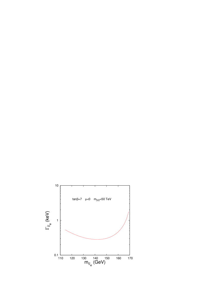
Figure 1: Total decay width of the electron-sneutrino (${\tilde{\nu}}_{e}$) as a function of the sneutrino mass. Here, we have fixed $m_{3/2}=50$ TeV and $\tan\beta=7$. The sign of $\mu$ is taken to be negative.

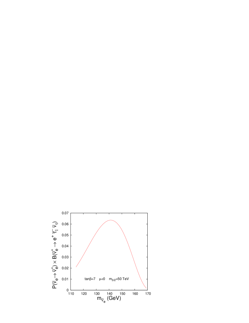
Figure 2: The probability of observing a positron in the decay of the ${\tilde{\nu}}_{e}$ (defined in Eq. (3)) as a function of $m_{{\tilde{\nu}}_{e}}$. Other parameter choices are the same as in Fig. 1.

Let us now show plots of the total decay width of the sneutrino/antisneutrino ($\Gamma_{\tilde{\nu}}$) and the probability of observing an opposite sign charged lepton in the final state of the decay of the sneutrino/antisneutrino given by Eq. (3). We have plotted these quantities for a fixed value of $m_{3/2}$ and $\tan\beta$, and the sign of $\mu$ is negative. The value of $m_{0}$ is changed in such a way that the condition (5) is satisfied. In Fig. 1, we have plotted the total decay width of the ${\tilde{\nu}}_{e}$ as a function of the sneutrino mass. The total width is calculated for the available three-body decay modes ${\tilde{\nu}}_{e}\rightarrow e^{-}{\tilde{\tau}}_{1}^{+}\nu_{\tau}$ and ${\tilde{\nu}}_{e}\rightarrow\nu_{e}{\tilde{\tau}}_{1}^{\pm}\tau^{\mp}$ mediated by virtual charginos and neutralinos, respectively. It is worth mentioning here that the neutralino-mediated modes ${\tilde{\nu}}_{e}\rightarrow\nu_{e}{\tilde{\tau}}_{1}^{-}\tau^{+}$ and ${\tilde{\nu}}_{e}\rightarrow\nu_{e}{\tilde{\tau}}_{1}^{+}\tau^{-}$ can, in general, have quite different partial decay widths. From Fig. 1, we can see that the total decay width is $\sim$ a few hundreds of eV in this region of the parameter space, being consistent with the requirement of observing a sizeable signal. In Fig. 2, we have plotted the probability of observing a positron in the decay of the ${\tilde{\nu}}_{e}$ (defined in Eq. 3) as a function of the mass of the ${\tilde{\nu}}_{e}$ for the same choice of parameters as in Fig. 1. The probability shows a peak for $m_{{\tilde{\nu}}_{e}}\approx 140$ GeV, since the total decay width $\Gamma_{{\tilde{\nu}}_{e}}$ is smallest for this value of $m_{{\tilde{\nu}}_{e}}$, and, hence, the quantity $x_{\tilde{\nu}}$ defined in Eq. (4) is largest for a fixed $\Delta m_{\tilde{\nu}}$. On the other hand, the branching ratio of ${\tilde{\nu}}_{e}^{*}\rightarrow e^{+}{\tilde{\tau}}_{1}^{-}{\bar{\nu}_{\tau}}$ does not change much for the range of $m_{{\tilde{\nu}}_{e}}$ shown in the figure. We can also see that the probability is not so small for this choice of parameters, and if the production cross section $e^{-}\gamma\rightarrow{\tilde{\chi}}_{1}^{-}{\tilde{\nu}}_{e}$ is large, a sizeable number of positron events can be seen.

Let us then move to discussing the physics of the electron-photon colliders and the production cross section of $\tilde{\chi}^{-}_{1}{\tilde{\nu}}_{e}$ with polarized and unpolarized beams. We will show the available region of the parameter space of the AMSB model where a reasonable number of signal events can be seen, while satisfying various experimental constraints. In addition, we will discuss the conditions under which the long-lived ${\tilde{\tau}}_{1}$s produce heavily ionizing charged tracks before decaying eventually to lepton and neutrino pairs so that they can be easily distinguished from other sleptons.

III $e^{-}\gamma$ collider and the photon spectrum

The way to obtain very high energy photon beams is to induce laser back-scattering off an energetic $e^{\pm}$ beam egammacollider . The reflected photon beam carries off only a fraction ($y$) of the energy of $e^{\pm}$ with

$$y_{max}=\frac{z}{1+z},~{}~{}~{}~{}z\equiv{\frac{4E_{b}E_{L}}{m^{2}_{e}}}{\rm cos}^{2}{\frac{\theta_{bL}}{2}},$$ (16)

where $E_{b(L)}$ are the energies of the incident electron/positron beam and the laser, respectively, and $\theta_{bL}$ is the incidence angle. The energy of the photon can be increased, in principle, by increasing the energy of the laser beam. However, a large $E_{L}$ (or, equivalently a large $z$) also enhances the probability of $e^{+}e^{-}$ pair creation through interactions between the laser and the scattered photon, consequently resulting in beam degradation. An optimal choice is $z=2(1+\sqrt{2})$, and this is the value we use in our analysis. The use of perfectly polarized electron and photon beams maximizes the signal cross section, though, in reality, it is almost impossible to achieve perfect polarizations. It is also extremely unlikely to have even near monochromatic high energy photon beams.

For an $e^{-}\gamma$ collider, the cross sections can be obtained by convoluting the fixed-energy cross sections ${\hat{\sigma}}({\hat{s}},P_{\gamma},P_{e^{-}})$ with the appropriate photon spectrum:

$$\sigma(s)=\int{\mathrm{d}y}{\mathrm{d}{\hat{s}}}{\frac{\mathrm{d}n}{\mathrm{d}y}}(P_{b},P_{L}){\hat{\sigma}}({\hat{s}},P_{\gamma},P_{e^{-}})\delta({\hat{s}}-ys),$$ (17)

where the photon polarization $P_{\gamma}$ is a function of $P_{b,L}$ and the momentum fraction $y$ through the relation $P_{\gamma}={P_{\gamma}}(y,P_{b},P_{L})$. In our analysis, we shall, for simplicity, consider circularly polarized laser beam scattering off polarized electron(positron) beams. The corresponding number-density $n(y)$ and average helicity for the scattered photons are then given by egammacollider ; egamma-tdr

$${\frac{dn}{dy}} = {\frac{2\pi\alpha^{2}}{m^{2}_{e}z\sigma_{C}}}C(y),$$

$${P_{\gamma}(y)} = {\frac{1}{C(y)}}\left[P_{b}\left\{{\frac{y}{1-y}}+y(2r-1)^{2}\right\}-P_{L}(2r-1)\left(1-y+{\frac{1}{1-y}}\right)\right],$$

$$C(y) \equiv {\frac{1}{1-y}}+(1-y)-4r(1-r)-P_{b}P_{L}rz(2r-1)(2-y),$$ (18)

where $r\equiv{y\over{z(1-y)}}$, and the total Compton cross section $\sigma_{C}$ provides the normalization.

It is also important to address another experimental issue regarding the long low-energy tail of the photon spectrum. In a realistic situation egamma-tdr , it is possible that these low-energy photons might not participate in any interaction. The harder back-scattered photons are emitted at smaller angles with respect to the direction of the initial electron, whereas softer photons are emitted at larger angles. Since the photons are distributed according to an effective spectrum (Eq. (18)), the low-energy photons which are produced at a wide angle are essentially thrown out, since they do not contribute significantly to any interaction. However, the exact profile of this effective spectrum is not simple, and it depends somewhat on the distance between the interaction point and the point where the laser photons are back-scattered and on the shape of the electron beam. Unfortunately, we are not in a position to include this effect in our simulations. It has been indicated in chou-cuypers that neglecting this effect does not change the total signal cross section to any significant extent.

Perfect polarization is relatively easy to obtain for the laser beam, and we shall use $|P_{L}|=1$. However, the same is not true for electrons or positrons, and we use $|P_{b}|=|P_{e^{-}}|=0.8$ as a conservative choice. Since we want to produce the sneutrino in this study, the $e^{-}$ should be left-polarized, i.e. $P_{e^{-}}=-0.8$. In order to improve the monochromaticity of the outgoing photons, the laser and the $e^{\pm}$ beam should be oppositely polarized berge , which means $P_{L}\times P_{b}<$ 0. In our analysis, we shall use both choices of polarizations consistent with $P_{L}\times P_{b}<$ 0.

IV Signal and backgrounds

As explained in the Introduction, we will focus on the production process egamma-prod $e^{-}\gamma\to{\tilde{\nu}}_{e}{\tilde{\chi}^{-}_{1}}$ and then look at the oscillation of the ${\tilde{\nu}}_{e}$ into a ${\tilde{\nu}}^{*}_{e}$. The resulting antisneutrino then decays through the three-body channel ${\tilde{\nu}}^{*}_{e}\to e^{+}{\tilde{\tau}}_{1}^{-}{\bar{\nu}}_{\tau}$ with a large branching ratio. The chargino $\tilde{\chi}^{-}_{1}$ subsequently decays into a ${\tilde{\tau}}_{1}^{-}$ and an antineutrino ($\bar{\nu}_{\tau}$). The neutrinos escape detection and give rise to an imbalance in momentum. The signal is then

$$e^{-}\gamma\to{\tilde{\nu}}_{e}{\tilde{\chi}^{-}_{1}}\to e^{+}+{\tilde{\tau}}_{1}^{-}+{\tilde{\tau}}_{1}^{-}+p_{T}/\;\>,$$ (19)

where the two ${\tilde{\tau}}_{1}^{-}$s are long-lived and can produce heavily ionizing charged tracks inside the detector after traversing a macroscopic distance. The positron serves as the trigger for the event. The probability that the chargino decays before travelling a distance $\delta$ is given by $P(\delta)=1-{\rm exp}(-\delta/L)$, where $L$ is the average decay length of the chargino. We assume that the ${\tilde{\tau}}_{1}^{-}$ decays through a tiny $R$-parity-violating coupling rpv-review $\lambda_{233}=5\times 10^{-9}$ into charged lepton + neutrino pairs so that a substantial number of events do have a reasonably large decay lengths for which the displaced vertex may be visible. At the end of this section, we will discuss the possible modifications in the signal event in order to accommodate a larger $R$-parity-violating coupling that will allow faster decay rates of the ${\tilde{\tau}}_{1}^{-}$s. Obviously, in such a situation, the Standard Model (SM) backgrounds would arise. We shall give numerical estimates of these SM backgrounds and discuss their implications.

The cross section of the signal event in Eq.(19) has been calculated in the narrow width approximation. We have calculated the $2\to 2$ differential cross section ${d\sigma(e^{-}\gamma\to{\tilde{\nu}}_{e}{\tilde{\chi}^{-}_{1}})}/{d\cos\theta}$ and then folded into it the probability of the sneutrino oscillation and proper branching fractions of the corresponding decay channels mentioned earlier to get the final state described above.

We select the signal events in Eq. (19) according to the following criteria$\colon$
$\bullet$ The transverse momentum of the positron must be large enough : $p^{e^{+}}_{T}>10$ GeV.
$\bullet$ The transverse momentum of the ${\tilde{\tau}}_{1}^{-}$s must satisfy $p^{{\tilde{\tau}}_{1}}_{T}>10$ GeV.
$\bullet$ The positron and both the staus must be relatively central, i.e. their pseudorapidities must fall in the range $|\eta^{{e^{+}},{\tilde{\tau}}_{1}}|<2.5$.
$\bullet$ The positron and the staus must be well-separated from each other$\colon$ i.e. the isolation variable $\Delta R\equiv\sqrt{(\Delta\eta)^{2}+(\Delta\phi)^{2}}$ (where $\eta$ and $\phi$ denote the separation in rapidity and the azimuthal angle, respectively) should satisfy $\Delta R>0.4$ for each combination.
$\bullet$ The missing transverse momentum $p_{T}/\;\>>10$ GeV.
$\bullet$ Both the heavily ionizing charged tracks due to the long-lived staus should have a length $\geq 5$ cm.

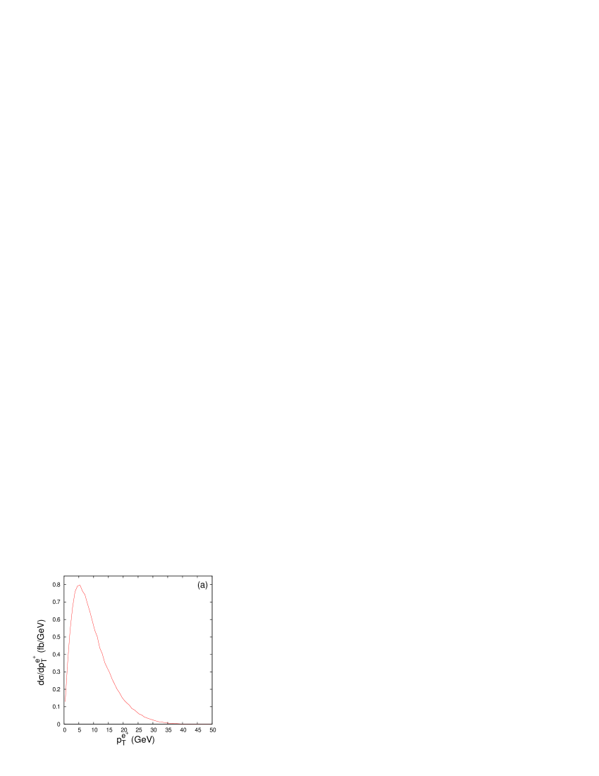
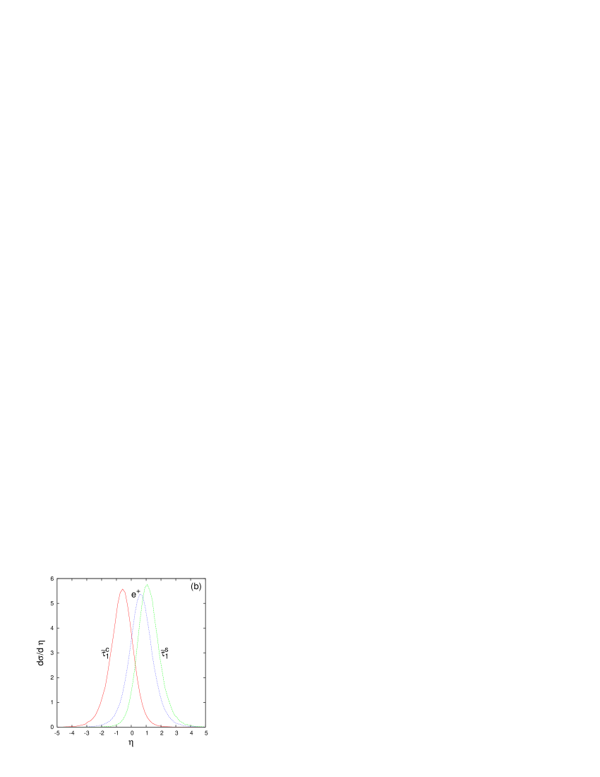
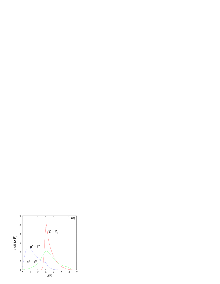
Figure 3: Kinematic distributions of signal events at a machine operating with $\sqrt{s_{ee}}$ = 500 GeV. The different plots correspond to (a) positron $p_{T}$; (b) rapidities; and (c) cone separations. Here, ${\tilde{\tau}}_{1}^{s}$ is the stau arising from the decay of the antisneutrino and ${\tilde{\tau}}_{1}^{c}$ is the other stau arising from the decay of the chargino. The choice of the beam polarization and other parameters are described in the text.

IV.1 The signal profile

In order to understand the profile of the signal we are looking for and to see the effects of the cuts we have employed, it is important to look at the kinematic distributions of various quantities. We will illustrate this for a sample point in the parameter space : $m_{0}=250$ GeV, $m_{3/2}=50$ TeV, $\tan\beta=7$ and $\mu<0$, leading to ($m_{\tilde{\chi}^{\pm}_{1}}$, $m_{{\tilde{\nu}}_{e}}$, $m_{{\tilde{\tau}}_{1}}$) $\approx$ (170, 142, 122) GeV. Beam polarization choices are $P_{L}=+1$, $P_{b}=P_{e^{-}}=-0.8$. As explained earlier, these distributions have been calculated in the narrow width approximation by convoluting the distributions of the “wrong-sign charged lepton” with those of the sneutrino from the $2\to 2$ process $e^{-}\gamma\to{\tilde{\nu}}_{e}{\tilde{\chi}^{-}_{1}}$. For such a choice of parameters, the total cross section is $\approx 10.26$ fb without any cuts for a machine operating at $\sqrt{s_{ee}}=500$ GeV. The transverse momentum of the positron in Fig. 3(a) shows its peak around 5 GeV and then falls sharply. This is due to the fact that the positron is coming from the decay of the ${\tilde{\nu}}_{e}^{*}$. Since the mass difference between the ${\tilde{\nu}}_{e}^{*}$ and the ${\tilde{\tau}}_{1}$ is not large, most of the positrons are softer. Hence, the requirement of the minimum positron transverse momentum of 10 GeV rejects quite a few signal events. However, this $p_{T}$ cut of 10 GeV is needed in order to trigger the event. Since the positron is coming out of the decay of the antisneutrino, it is quite central, which can also be seen from its rapidity distribution in Fig. 3(b). On the other hand, one of the staus comes from the decay of the chargino and the other one comes from the decay of the sneutrino. The one (${\tilde{\tau}}_{1}^{s}$) arising from the sneutrino decay shows quite similar behaviour as the positron, whereas the other (${\tilde{\tau}}_{1}^{c}$) arising from the chargino decay, though being quite central, is somewhat boosted in the opposite direction (Fig. 3(b)). One can immediately understand that the ${\tilde{\tau}}_{1}^{c}$ is well-separated from the positron and the other stau (${\tilde{\tau}}_{1}^{s}$). This feature is evident from the distribution shown in Fig. 3(c). This conclusion holds almost over the entire allowed parameter space which we are considering. On the other hand, the angular separation between the positron and ${\tilde{\tau}}_{1}^{s}$ is much smaller, and the position of the peak moves slightly depending on the point chosen in the allowed parameter space. Because of the choice of a very small $R$-parity-violating coupling, both the staus leave a substantial track, and, for most of the events, the decay lengths are greater than 10 cm. Some of the events can have charged tracks which may extend up to a meter or greater than that.

IV.2 The SUSY backgrounds

As one can see, due to the presence of these heavily ionizing charged tracks, the signal is entirely free of any Standard Model (SM) background. However, there are backgrounds from SUSY processes. One possibility is the associated production of the left-selectron (${\tilde{e}}_{L}^{-}$) and the lightest neutralino (${\tilde{\chi}}^{0}_{1}$). If the mass of the left-selectron is larger than the mass of the lighter chargino, then it may subsequently decay into an ($e^{-}$ + ${\tilde{\chi}}^{0}_{1}$) pair or a (${\tilde{\chi}}^{-}_{1}$ + $\nu_{e}$) pair with the branching fractions $B({\tilde{e}}_{L}^{-}\rightarrow e^{-}+{\tilde{\chi}}^{0}_{1})\approx 33-39$ % and $B({\tilde{e}}_{L}^{-}\rightarrow\nu_{e}+{\tilde{\chi}}^{-}_{1})\approx 60-66$ %, due to the fact that both ${\tilde{\chi}}^{0}_{1}$ and ${\tilde{\chi}}^{-}_{1}$ are predominantly winos. Two-body decays into heavier neutralinos (charginos) are kinematically forbidden for most of the parameter space. In order to have the same visible final state as in the case of our signal, we concentrate on the neutrino-chargino channel. The lightest neutralino (${\tilde{\chi}}^{0}_{1}$) may decay into an electron-neutrino ($\nu_{e}$) and the associated antisneutrino (${\tilde{\nu}}_{e}^{*}$). Due to the choice of our spectrum in Eq. (5), ${\tilde{\chi}}^{0}_{1}$ always has this two-body mode available. The resulting antisneutrino can go to the three-body channel ${\tilde{\nu}}_{e}^{*}\rightarrow e^{+}{\tilde{\tau}}^{-}_{1}{{\bar{\nu}}_{\tau}}$, and the chargino arising from the selectron decay may go into a (${\tilde{\tau}}_{1}^{-}+{\bar{\nu}}_{\tau}$) pair. The final background event is then $e^{-}\gamma\rightarrow{\tilde{e}}_{L}^{-}{\tilde{\chi}^{0}_{1}}\rightarrow e^{+}{\tilde{\tau}}^{-}_{1}{\tilde{\tau}}^{-}_{1}{\nu_{e}}{{\bar{\nu}}_{\tau}}{\nu_{e}}{{\bar{\nu}}_{\tau}}$, where the neutrinos give rise to the missing transverse momentum $p_{T}/\;\>$.

In order to compare the strength of the background and the signal event, let us give an example. For $m_{0}=255$ GeV, $m_{3/2}=50$ TeV, $\tan\beta=7$ and $\mu<0$, the spectrum is $m_{{\tilde{e}}_{L}}=171.4$ GeV, $m_{{\tilde{\nu}}_{e}}=151.1$ GeV, $m_{{\tilde{\chi}}_{1}^{-}}=170.1$ GeV, $m_{{\tilde{\chi}}_{1}^{0}}=169.94$ GeV and $m_{{\tilde{\tau}}_{1}}=131.8$ GeV. After imposing our cuts at $\sqrt{s_{ee}}=500$ GeV, the surviving background is 0.48 fb and the signal is 2.33 fb. Here, the polarization choices are the same as in the previous subsection. If we now calculate the signal significance $\equiv$ $N_{e}/\sqrt{N_{e}+N_{B}}$, where $N_{e}$ is the number of signal events and $N_{B}$ is the number of background events, then, for this particular example, the ratio is much greater than 5 for an integrated luminosity of 500 ${\rm fb}^{-1}$. If we increase the value of $m_{0}$, then the masses of both the ${\tilde{e}}_{L}$ and the ${\tilde{\nu}}_{e}$ increase, and, as a result, the signal as well as the background cross sections decrease. However, the signal significance always remains greater than 5. On the other hand, if we keep $m_{0}$ fixed and change the value of $m_{3/2}$ in such a way that ${\tilde{e}}_{L}$ is always heavier than ${\tilde{\chi}}_{1}^{-}$ and ${\tilde{\chi}}_{1}^{0}$, then the signal significance remains again greater than 5. One of the reasons for this small cross section of the background event is that the branching ratio $B({\tilde{\chi}}_{1}^{0}\rightarrow\nu_{e}{\tilde{\nu}}_{e}^{*}$) is very small (less than 10 %). It is worth mentioning that the decay ${\tilde{\chi}}_{1}^{0}\rightarrow{\bar{\nu}}_{e}{\tilde{\nu}}_{e}$ could contribute to the signal through the ${\tilde{\nu}}_{e}$–${\tilde{\nu}}_{e}^{*}$ oscillation, but this process is further suppressed by the small oscillation probability (less than 0.1) and is hence negligible.

In the case when ${\tilde{e}}_{L}^{-}$ is lighter than ${\tilde{\chi}}_{1}^{-}$ and ${\tilde{\chi}}_{1}^{0}$, it can decay into the chargino-mediated three-body mode ${\tilde{e}}_{L}^{-}\rightarrow\nu_{e}{\tilde{\tau}}_{1}^{-}{\bar{\nu}}_{\tau}$, which contributes to the background. In this case, one should notice that ${\tilde{\chi}}_{1}^{0}$ goes to the two-body mode ${\tilde{\nu}}_{e}^{*}\nu_{e}$ with a branching ratio smaller than in the earlier case. There are other three-body decay modes available for the left-selectron in this case, namely, ${\tilde{e}}_{L}^{-}\rightarrow e^{-}\tau^{\pm}{\tilde{\tau}}_{1}^{\mp}$, ${\tilde{e}}_{L}^{-}\rightarrow{\nu_{e}}{\ell^{-}}{\tilde{\nu}}^{*}_{\ell}$, ${\tilde{e}}_{L}^{-}\rightarrow e^{-}{\nu_{\mu,\tau}}{{\tilde{\nu}}_{\mu,\tau}^{*}},e^{-}{\bar{\nu}_{\mu,\tau}}{{\tilde{\nu}}_{\mu,\tau}}$ and ${\tilde{e}}_{L}^{-}\rightarrow{\tilde{\nu}}_{e}\ell^{-}{\bar{\nu}}_{\ell}$ where $\ell=e,\mu,\tau$. Here, we have neglected the three-body decays involving ${\tilde{e}}_{R}$ and ${\tilde{\mu}}_{R}$ in the final state. From the above discussion, we can conclude that the cross section for the background event still remains quite small in the case when ${\tilde{e}}_{L}$ is lighter than ${\tilde{\chi}}_{1}^{-}$ and ${\tilde{\chi}}_{1}^{0}$. On the other hand, the signal also suffers a suppression due to a smaller branching ratio of ${\tilde{\chi}}^{-}_{1}$ in the (${\tilde{\tau}}_{1}^{-}+\nu_{\tau}$) mode. However, this suppression is such that the ratio $N_{e}/\sqrt{N_{e}+N_{B}}$ always remains greater than or equal to 5.

Another source of background could be the associated production $e^{-}\gamma\rightarrow{\tilde{e}}_{L}^{-}{\tilde{\chi}}^{0}_{2}$. However, this production process is kinematically forbidden for the entire region of the parameter space we are investigating for a machine operating at $\sqrt{s_{ee}}$ = 500 GeV. For a $\sqrt{s_{ee}}$ = 1 TeV collider, this process is allowed, but the production cross section is too small to contribute significantly. The 2 $\rightarrow$ 3 process $e^{-}\gamma\rightarrow{\nu_{e}}{{\tilde{e}}_{L}^{-}}{\tilde{\nu}}_{e}^{*}$ could also contribute to the background, but the production cross section in this case is very small ($<{\mathcal{O}}(10^{-2})$ fb) like-sign-rp .

IV.3 The signal strength and the parameter space

Let us now discuss the signal event in more detail. The number of signal events and the kinematical distributions depend crucially on the sneutrino and the chargino masses and also on the mass of ${\tilde{\tau}}_{1}$. In our analysis, the evolution of gauge and Yukawa couplings as well as that of scalar masses are computed using two-loop renormalization group equations (RGE) martin-vaughn . We have also incorporated the unification of gauge couplings at the scale $M_{G}\sim 2\times 10^{16}$ GeV with $\alpha_{3}(M_{Z})\approx 0.118$. The boundary conditions for the scalar masses are given at the unification scale via Eq. (7). The magnitude of the higgsino mass parameter $\mu$ is computed from the requirement of a radiative electroweak symmetry breaking and at the complete one-loop level of the effective potential potential . The optimal choice of the renormalization scale is expressed in terms of the masses of the top-squarks through the relation $Q^{2}=m_{{\tilde{t}}_{1}}m_{{\tilde{t}}_{2}}$. We have also included the supersymmetric QCD corrections to the bottom-quark mass susy-qcd , which is significant for large $\tan\beta$. It should be noted at this point that gaugino masses and trilinear scalar couplings can be computed from the expressions in Eqs. (8) and (9) at any scale once the appropriate values of the gauge and Yukawa couplings at that scale are known. A particularly interesting feature of the mAMSB model is that the lighter chargino ${\tilde{\chi}}^{\pm}_{1}$ and the lightest neutralino ${\tilde{\chi}}^{0}_{1}$ are both almost exclusively a wino and, hence, nearly mass-degenerate. A small mass difference is generated from the tree-level gaugino-higgsino mixing as well as from the one-loop corrections to the chargino and the neutralino mass matrices mass-diff . The numerical results of the spectrum of mAMSB model have been obtained using the fortran codes developed in muong-2-1 and in the first two references of amsb-linearee . We have checked that our results agree with those of previous authors amsb-hadron1 for a few sample choices of parameters.

It is important to look at the total number of signal events as a function of the model parameters with the condition on the spectrum given in Eq. (5). In order to do this, we will fix the value of $\tan\beta$ and take the signature of $\mu$ to be negative and then allow $m_{0}$ and $m_{3/2}$ to vary in a region which satisfies the experimental constraints on the sparticle masses. Later on, we will also discuss how the total cross section changes with $\tan\beta$ and the sign of $\mu$. As above, we make a specific choice for the beam polarization, namely, $P_{L}=+1$, $P_{b}=P_{e^{-}}=-0.8$.

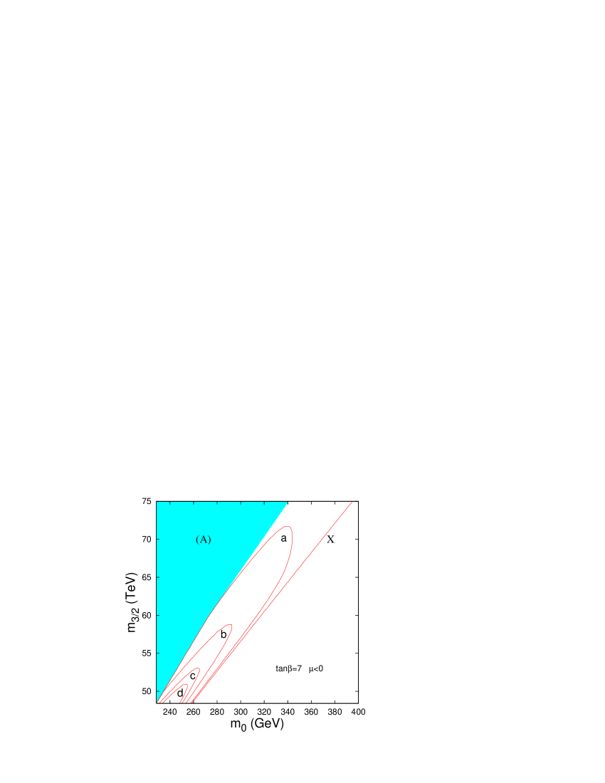
Figure 4: Parameter regions with $\tan\beta=7$ and $\mu<0$. The area (A) represents the parameter region forbidden by the stau mass bound. The mass spectrum (5) is obtained in the region between the area (A) and the line X. Assuming an integrated luminosity of $500$ fb^-1 at $\sqrt{s_{ee}}=500$ GeV, the numbers of positron events per year inside the contours are: (a) $N_{e}\geq 50$, (b) $N_{e}\geq 500$, (c) $N_{e}\geq 1000$ and (d) $N_{e}\geq 1300$ for $(m_{\nu})^{0}_{ee}$ = 0.079 eV so that the total contribution $(m_{\nu})_{ee}\approx$ 0.2 eV, while satisfying $N_{e}\geq 5\sqrt{N_{e}+N_{\mathrm{B}}}$.

In Fig. 4, we show our results for the total number of positron events for a machine operating at $\sqrt{s_{ee}}$ = 500 GeV with 500 fb^-1 integrated luminosity, after imposing the kinematical cuts discussed above. The region marked by (A) corresponds to a lighter stau mass of less than 86 GeV PDG . The area below the line X does not satisfy the mass hierarchy of Eq. (5). Thus, the allowed region in the ($m_{0}-m_{3/2}$) plane is the one between the area (A) and the line X. The other experimental constraints PDG which we have used are the mass of the lighter chargino ($m_{\tilde{\chi}^{\pm}_{1}}>$ 104 GeV), the mass of the sneutrino ($m_{\tilde{\nu}}>$ 94 GeV) and the mass of the lightest Higgs boson haber-carena ($m_{h}>$ 113 GeV). Apart from these direct bounds, one should also consider the constraints on the parameter space arising from the virtual exchange contributions to low-energy observables. For example, the constraints on the minimal AMSB model parameters from the measurement of muon anomalous magnetic moment have been studied in several works muong-2-1 ; muong-2-2 ; muong-2-3 . However, the numerical results of those papers should be modified due to the reevaluation of the light by light hadronic contribution lightbylight and the results published by the E821 experiment E821 . In addition, one should bear in mind that the theoretical calculation of the SM contribution to muon $(g-2)$ has many remaining theoretical uncertainties. The measurement of the rare decay $\Gamma(B\rightarrow X_{s}\gamma)$ can set additional bounds muong-2-2 ; muong-2-3 on the parameters, but they are not very restrictive. Bounds can also be obtained by demanding that the electroweak vacuum corresponds to the global minimum of the scalar potential vacuumstability . However, as long as it can be ensured that the local minimum has a life time longer than the present age of the Universe, these additional bounds can be evaded universe .

We have used the value of $\tan\beta=7$, and the sign of $\mu$ is taken to be negative. It has already been mentioned that, in the AMSB scenario, the positron events in an $e^{-}\gamma$ collider via the sneutrino-antisneutrino mixing can provide information on the neutrino mass matrix elements $(m_{\nu})_{ee}$. In Fig. 4, we have chosen the value of $(m_{\nu})_{ee}^{0}=0.079$ eV which corresponds to $(m_{\nu})_{ee}\approx$ 0.2 eV. Later on, we will make comments on the smallest value of $(m_{\nu})_{ee}$ which can be probed in this scenario. In this figure, we have plotted contours of total number of positron events $N_{e}$, starting with $N_{e}$ = 50. It is evident from this figure that an experiment of this type can easily explore $m_{3/2}$ as high as $\approx$ 72 TeV whereas the reach in $m_{0}$ is $\approx$ 340 GeV for a negative $\mu$, $\tan\beta$=7 and $(m_{\nu})_{ee}\approx$ 0.2 eV. Even with an integrated luminosity of 100 fb^-1, it is possible to explore values of $m_{3/2}$ and $m_{0}$ up to $\approx$ 64 TeV and 315 GeV, respectively, with $N_{e}\geq 50$.

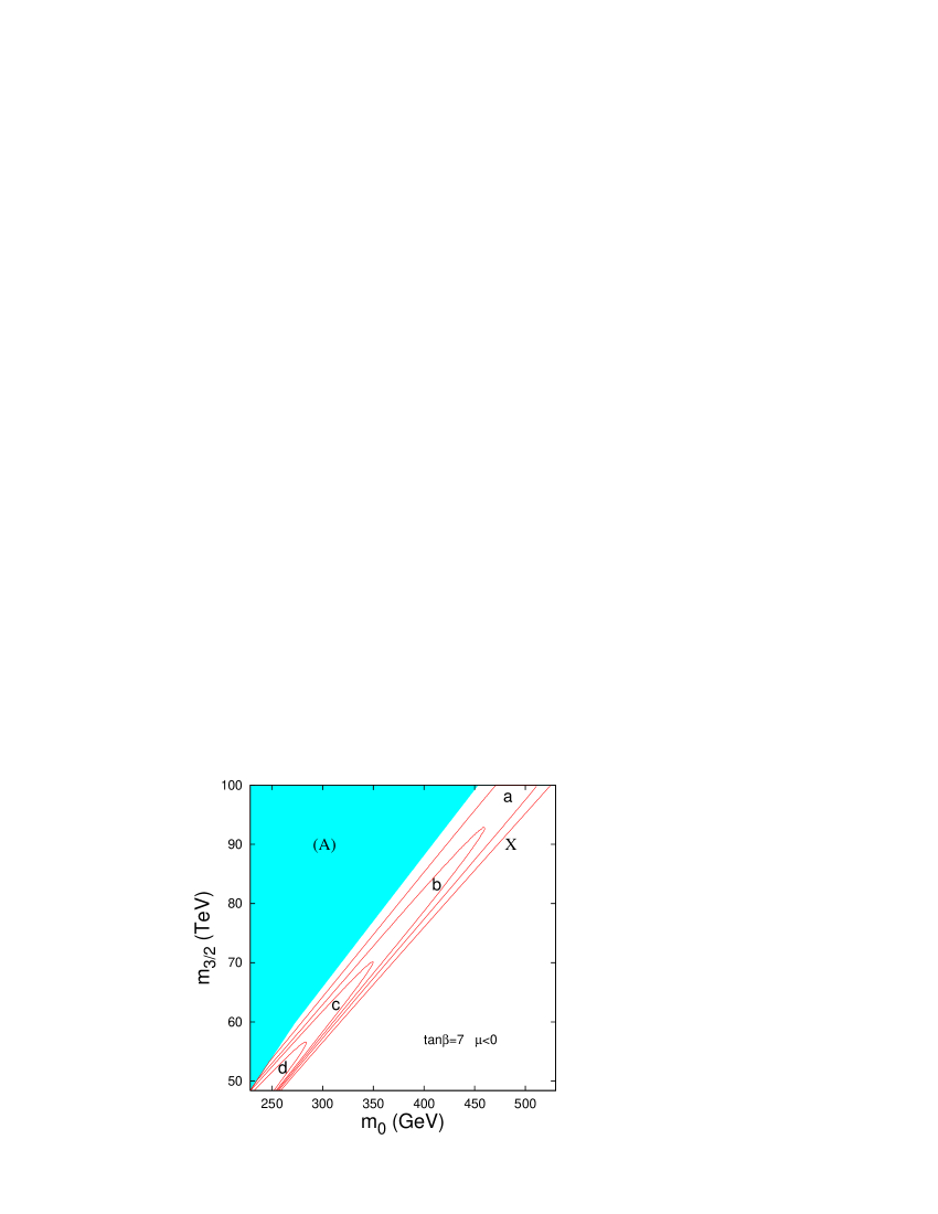
Figure 5: Parameter regions with $\tan\beta=7$ and $\mu<0$. The area (A) represents the parameter region forbidden by the stau mass bound. The mass spectrum (5) is obtained in the region between the area (A) and the line X. Assuming an integrated luminosity of $500$ fb^-1 at $\sqrt{s_{ee}}=1$ TeV, the numbers of positron events per year inside the contours are: (a) $N_{e}\geq 100$, (b) $N_{e}\geq 200$, (c) $N_{e}\geq 300$ and (d) $N_{e}\geq 500$ for $(m_{\nu})^{0}_{ee}$ = 0.079 eV so that the total contribution $(m_{\nu})_{ee}\approx$ $0.2$ eV, while satisfying $N_{e}\geq 5\sqrt{N_{e}+N_{\mathrm{B}}}$.

In Fig. 5, we show a similar plot in the ($m_{0}$ – $m_{3/2}$) plane for a machine operating at $\sqrt{s}$ = 1 TeV with other inputs remaining the same. We can see similar features in both the Figures 4 and 5, with the obvious enhancement in the reach in the latter case.

So far, we have discussed the strength of the signal for a fixed value of the parameter $\tan\beta$. Let us now see how the signal cross section changes with varying $\tan\beta$. For a fixed $m_{3/2}$ and with increasing $\tan\beta$, a larger value of $m_{0}$ is required to obtain the spectrum (5) for both choices of the sign of $\mu$. This leads to a larger value of $m_{{\tilde{\nu}}_{e}}$. On the other hand, $m_{{\tilde{\tau}}_{1}}$ becomes smaller due to a stronger left-right mixing in the stau sector. Thus, the ratio ${m_{{\tilde{\nu}}_{e}}}/{m_{{\tilde{\tau}}_{1}}}$ increases with $\tan\beta$, making the sneutrino decay width $\Gamma_{{\tilde{\nu}}_{e}}$ an increasing function of $\tan\beta$. Hence, in order to get a sizeable number of positron events $N_{e}$, one needs a small value of the parameter $\tan\beta$ for a fixed neutrino mass. This feature has also been observed in Ref. like-sign-norp . For $\mu>$ 0, the Higgs boson mass is a bit lower, so we need a higher $\tan\beta$ for a fixed $m_{3/2}$ to satisfy the constraint on the light Higgs boson mass $m_{h}>113$ GeV. This makes the number of positron events very small. When $\tan\beta$ is fixed, the allowed region in the $m_{0}$ – $m_{3/2}$ plane is shortened for $\mu>0$, since a higher value of $m_{3/2}$ is required in order to satisfy the Higgs boson mass bound. For a negative $\mu$, the requirement of observing the signal with at least $5\sigma$ significance implies that the highest allowed value of $\tan\beta$ is $\approx 8.1$ with a machine operating at $\sqrt{s_{ee}}=500$ GeV, and $\tan\beta$ is $\approx 8.0$ for a machine with $\sqrt{s_{ee}}$ = 1 TeV. The lowest allowed value of $\tan\beta$ for a fixed $m_{3/2}$ is limited by the Higgs boson mass bound. For a negative $\mu$, we can have $\tan\beta$ as low as $\approx 4.9$, which will still produce an acceptable Higgs boson mass and at least $5\sigma$ signal significance for $\sqrt{s_{ee}}=500$ GeV. For a value of $\tan\beta$ as low as 4.9, it is notable that the value of $m_{0}$ and $m_{3/2}$ should be quite high ($m_{0}\approx 375$ GeV and $m_{3/2}\approx 88$ TeV) in order to have enough signal events. For $\sqrt{s_{ee}}=1$ TeV, the lowest allowed value of $\tan\beta$ is approximately the same. In order to have $5\sigma$ signal significance for a positive $\mu$, we must have $\sqrt{s_{ee}}=1$ TeV in which case the $\tan\beta$ range is quite small $\approx$ $6.1$–$6.3$, while the value of $m_{3/2}$ is of the order of $100$ TeV and $m_{0}$ is in the range $460$–$590$ GeV.

( $m_{0}~{}{\rm(GeV)},~{}m_{3/2}~{}{\rm(TeV)},~{}\tan\beta$ )	(250, 50, 7)			(350, 70, 7)
( $m_{\tilde{\chi}^{-}_{1}},m_{{\tilde{\nu}}_{e}},m_{{\tilde{\tau}}_{1}}~{})~{}{\rm(GeV)}$	( 170.1, 142.5, 121.9 )			( 239.6, 208.9, 179.3)
	$(P_{L},P_{b},P_{e^{-}})$			$(P_{L},P_{b},P_{e^{-}})$
	($-,+,-$)	($+,-,-$)	($0,0,0$)	($-,+,-$)	($+,-,-$)	($0,0,0$)
Total $\sigma$ (without cuts) (fb)	7.15	5.93	3.21	1.29	1.45	0.66
Total $\sigma$ (with cuts) (fb)	2.12	1.58	0.92	0.56	0.59	0.28

Table 1: Illustrating the effects of various polarization choices on the signal cross sections for two specimen points in the parameter space and for $\sqrt{s_{ee}}=1$ TeV. In either case, $\mu<0$. Whenever nonzero, $|P_{L}|=1$, $|P_{b}|=|P_{e^{-}}|=0.8$.

In order to discuss the effect of the beam polarizations, we choose two sample points in the parameter space and show the results in Table 1 for a machine with $\sqrt{s_{ee}}$ = 1 TeV. One can see that the cross sections for polarized beams are larger than the unpolarized ones. The effect of the cuts can also be seen. Depending on the choice of the parameters, the kinematical cuts can reduce the number of events by more than 50 %.

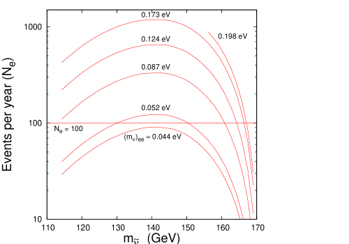
Figure 6: Number of events ($N_{e}$) per year (with an integrated luminosity of 500 $\mathrm{fb}^{-1}$) as a function of $m_{{\tilde{\nu}}_{e}}$ for different choices of $(m_{\nu})^{0}_{ee}$ as dicussed in the text. Here, $\tan\beta=7$, $\mu<0$ and $m_{3/2}$ = 50 TeV. The values of the total contribution $(m_{\nu})_{ee}$ corresponding to each line are shown in the figure. The horizontal line stands for $N_{e}$ = 100 satisfying $N_{e}\geq 5\sqrt{N_{e}+N_{\mathrm{B}}}$.

Let us now discuss the change in the number of events when $(m_{\nu})^{0}_{ee}$ is varied in such a way that it is consistent with the upper limit of $0.2$ eV for the total contribution $(m_{\nu})_{ee}$. For the purpose of this discussion, we choose a machine operating at $\sqrt{s_{ee}}$ = 500 GeV. It is evident from our discussion so far that larger values of $(m_{\nu})^{0}_{ee}$ give a larger cross section. This is also shown in Fig. 6 for a sample choice of $m_{3/2}$ = 50 TeV, $\tan\beta$ = 7 and $\mu<$ 0. Assuming an integrated luminosity of 500 $\mathrm{fb}^{-1}$, we have plotted the number of events per year as a function of $m_{{\tilde{\nu}}_{e}}$ for different choices of $(m_{\nu})^{0}_{ee}$. The curves from below correspond to $(m_{\nu})^{0}_{ee}$ = 0.018 eV, 0.021 eV, 0.035 eV, 0.05 eV, 0.07 eV and 0.081 eV. The corresponding values of the total contribution $(m_{\nu})_{ee}$ are shown in the figure. The horizontal line gives $N_{e}$ = 100 per year. This figure tells us that if we demand the value of $N_{e}$ to be $\geq$ 100, so that the signal significance is $\geq$ 5$\sigma$, then we can probe the value of $(m_{\nu})_{ee}$ down to $\approx$ 0.05 eV. On the other hand, the current upper limit of 0.2 eV on $(m_{\nu})_{ee}$ sets the upper limit of $(m_{\nu})^{0}_{ee}\approx$ 0.081 eV. The topmost curve in this figure starts from a slightly higher value of $m_{{\tilde{\nu}}_{e}}$, since the bound on $(m_{\nu})_{ee}$ is not satisfied before that. This figure can also be used to extract the value of $(m_{\nu})_{ee}$ with the knowledge of the number of events and other masses.

Finally, we will discuss the situation when a larger $R$-parity-violating (RPV) coupling is present. We shall assume that a single RPV coupling is dominant at a time, and our choice is $\lambda_{233}$. The reason behind this choice is that it will not affect the total decay width of ${\tilde{\nu}}_{e}^{*}$, since otherwise the $\Delta L$ = 2 effect will be diluted. The coupling $\lambda_{233}$ also allows observation of muons and taus in the final state from the decay of the ${\tilde{\tau}}_{1}^{-}$s, so that they can be clearly distinguished (assuming 100$\%$ detection efficiency) from the isolated $e^{+}$ produced due to the sneutrino mixing phenomena. The upper bound on the coupling $\lambda_{233}$ is given by rpv-bounds

$$|\lambda_{233}|<0.070\times\frac{m_{{\tilde{\tau}}_{R}}}{100~{}{\mathrm{GeV}}}.$$ (20)

The bound in Eq. (20) has been obtained from measurements of $R_{\tau}=\Gamma(\tau\rightarrow e\nu\bar{\nu})/\Gamma(\tau\rightarrow\mu\nu\bar{\nu})$ and $R_{\tau\mu}=\Gamma(\tau\rightarrow\mu\nu\bar{\nu})/\Gamma(\mu\rightarrow e\nu\bar{\nu})$. Using this upper limit on $\lambda_{233}$, we see that the ${\tilde{\tau}}_{1}^{-}$s will decay promptly to either a $(\tau+\nu_{\mu})$ pair or a $(\mu+\nu_{\tau})$ pair. Taking into account all possible final states involving $\mu$ and/or $\tau$, the signal event in this situation looks like $e^{-}\gamma\rightarrow e^{+}\ell^{-}\ell^{-}+p_{T}/\;\>$ where $\ell=\mu,\tau$.

The SM background to this process arises from the resonant production of three $W^{\pm}$ bosons through the $2\rightarrow 4$ process $e^{-}\gamma\rightarrow W^{-}W^{-}W^{+}\nu_{e}$ and the subsequent decays of the $W^{\pm}$s. The background to the signal $e^{-}\gamma\rightarrow e^{+}\ell^{-}\ell^{-}+p_{T}/\;\>$ originates when the $W^{+}$ decays through $W^{+}\rightarrow e^{+}\nu_{e}$ and the two $W^{-}$s decay through $W^{-}\rightarrow\ell^{-}{\bar{\nu}}_{\ell}$. This process has already been calculated in Ref. pilaftsis for two values of the c.m. energy, namely, $\sqrt{s_{\mathrm{ee}}}$ = 500 GeV and $\sqrt{s_{\mathrm{ee}}}$ = 1 TeV. As can be seen from the Table 1 of Ref. pilaftsis , the background cross section for $\sqrt{s_{\mathrm{ee}}}$ = 500 GeV is $\approx$ 0.0089 fb (after dividing the number in the table by $B(W^{-}W^{-}\rightarrow hadrons)$ and multiplying by $B(W^{-}W^{-}\rightarrow(\mu+\tau))$, and that for $\sqrt{s_{\mathrm{ee}}}=1$ TeV is $\approx 0.1257$ fb. One should note here that these numbers for the background cross sections are without any cuts and should be reduced further after imposing suitable kinematical cuts. It should be mentioned here that the SUSY background analysis remains almost the same as discussed in the subsection IVB but now with prompt decays of the ${\tilde{\tau}}_{1}^{-}$s.

In order to look at the signal to background ratio in this case, let us choose $\sqrt{s_{ee}}=500$ GeV and two widely separated points in the parameter space$\colon$

(A) $m_{0}=255$ GeV, $m_{3/2}=50$ TeV, $\tan\beta=7$ and $\mu<0$; and
(B) $m_{0}=310$ GeV, $m_{3/2}=60$ TeV, $\tan\beta=7$ and $\mu<0$.

The polarization choices are the same as in the subsection IVA. The signal cross section for the point (A) is 3.3 fb (with only a cut on the positron $p_{T}$, which is the most effective one, and on the positron pseudorapidity) and the SUSY background cross section is 0.67 fb. Combining this background cross section with the SM background mentioned above, we see that the signal to background ratio is greater than $5\sigma$. Similarly, for the point (B), the signal cross section is 0.425 fb and the SUSY background cross section is 0.328 fb. Again, we see that the ratio $N_{e}/\sqrt{N_{e}+N_{B}}$ is greater than 5. Thus, even in the case of a larger RPV coupling, we can explore an appreciable region in the parameter space of our interest with the signal described above. We have also performed a similar analysis for a $\sqrt{s_{ee}}$ = 1 TeV collider, and, once again, it shows that a significant region in the parameter space of mAMSB model with a spectrum given in Eq. (5) can be probed by this signal.

V Conclusion

In conclusion, we have discussed the potential of an electron-photon collider to investigate the signature of $\tilde{\nu}_{e}$–${\tilde{\nu}}_{e}^{*}$ mixing in an AMSB model which can accommodate $\Delta L=2$ Majorana neutrino masses. A very interesting feature of such models is that the sneutrino-antisneutrino mass splitting $\Delta m_{\tilde{\nu}}$ is naturally large and is ${\mathcal{O}}({4\pi{m_{\nu}}}/\alpha)$. On the other hand, the total decay width of the sneutrino is sufficiently small in a significant region of the allowed parameter space of the model. These two features enhance the possibility of observing sneutrino oscillation signal in various colliders. We have demonstrated that the associated production of the lighter chargino and the sneutrino at an $e^{-}\gamma$ collider could provide a very clean signature of such a scenario.

The signal event consists of an energetic positron (resulting from the oscillation of a ${\tilde{\nu}}_{e}$ into a ${\tilde{\nu}}_{e}^{*}$), which serves as the trigger, two macroscopic heavily ionizing charged tracks in the detector coming from the long-lived staus and a large missing transverse momentum. Due to the presence of these macroscopic charged tracks in combination with the energetic positron, the signal is free of any Standard Model backgrounds. The backgrounds from supersymmetric processes are present, but they are small and become even smaller with the cuts we have imposed. Consequently, with an integrated luminosity of 500 fb^-1, one could see as many as 1300 signal events in some region of the parameter space for a machine operating at $\sqrt{s_{ee}}$ = 500 GeV with polarized beams. We have also seen that the signal significance is $\geq 5\sigma$ for almost the entire allowed region of parameter space. In the case of a $\sqrt{s_{ee}}$ = 1 TeV collider, the features are similar with an obvious enhancement in the reach. The signal cross section depends also on $(m_{\nu})_{ee}$, and, obviously, we get the best result with the value of $(m_{\nu})_{ee}$ (including both tree and one-loop contribution) close to its present upper limit. We have also discussed the effects on the signal cross section when lowering the value of $(m_{\nu})_{ee}$. This way, the signal discussed in this paper can be used to determine $(m_{\nu})_{ee}$ which provides important information on a particular combination of the neutrino masses and mixing angles, which is not possible to obtain from neutrino oscillation experiments. Slightly lower values of $\tan\beta$ ($\lower 2.15277pt\hbox{$\>\buildrel<\over{\sim}\>$}9$) and a negative $\mu$ are preferred to get a sizeable number of signal events. Taking into account various experimental constraints and demanding that the signal significance should be $\geq 5\sigma$, we see that the lower limit on $\tan\beta$ is $\approx 4.9$. We have also discussed the possible effects on the signal when a larger $R$-parity-violating coupling is introduced. Numerical estimates of the Standard Model backgrounds in this case have also been provided.

- (1) For recent reviews on neutrino physics, see, e.g. G. Altarelli, hep-ph/0508053 and B. Kayser, hep-ph/0506165.
- (2) M. Hirsch, H.V. Klapdor-Kleingrothaus, and S.G. Kovalenko, Phys. Lett. B398, 311 (1997).
- (3) Y. Grossman and H.E. Haber, Phys. Rev. Lett. 78, 3438 (1997).
- (4) Y. Grossman and H.E. Haber, Phys. Rev. D59, 093008 (1999); ibid. 63, 075011 (2001).
- (5) E.J. Chun, Phys. Lett. B525, 114 (2002).
- (6) S. Davidson and S.F. King, Phys. Lett. B445, 191 (1998).
- (7) For reviews, see, e.g. P.J. Franzini, Phys. Rep. 173, 1 (1989); H.R. Quinn, Eur. Phys. J. C 3, 555 (1998).
- (8) N. Arkani-Hamed, H-C. Cheng, J.L. Feng, and L.J. Hall, Phys. Rev. Lett. 77, 1937 (1996).
- (9) A. Gould, B.T. Draine, R.W. Romani, and S. Nussinov, Phys. Lett. B238, 337 (1990); G. Starkman, A. Gould, R. Esmailzadeh, and S. Dimopoulos, Phys. Rev. D41, 3594 (1990); T. Hemmick et al., Phys. Rev. D41, 2074 (1990); P. Verkerk et al., Phys. Rev. Lett. 68, 1116 (1992).
- (10) S. Kolb, M. Hirsch, H.V. Klapdor-Kleingrothaus, and O. Panella, Phys. Rev. D64, 115006 (2001).
- (11) K. Choi, K. Hwang, and W.Y. Song, Phys. Rev. Lett. 88, 141801 (2002).
- (12) M. Hirsch, H.V. Klapdor-Kleingrothaus, S. Kolb, and S.G. Kovalenko, Phys. Rev. D57, 2020 (1998).
- (13) S. Bar-Shalom, G. Eilam, and A. Soni, Phys. Rev. Lett. 80, 4629 (1998); Phys. Rev. D59, 055012 (1999).
- (14) L. Randall and R. Sundrum, Nucl. Phys. B557, 79 (1999); G.F. Giudice, M.A. Luty, H. Murayama, and R. Rattazzi, J. High Energy Phys. 12, 027 (1998).
- (15) A. Pomarol, R. Rattazzi, J. High Energy Phys. 05, 013 (1999); E. Katz, Y. Shadmi, Y. Shirman, J. High Energy Phys. 08, 015 (1999); R. Rattazzi, A. Strumia, J.D. Wells, Nucl. Phys. B576, 3 (2000); Z. Chacko, M. Luty, E. Pontón, Y. Shadmi, Y. Shirman, Phys. Rev. D64, 055009 (2001); Z. Chacko, M.A. Luty, I. Maksymyk, E. Pontón, J. High Energy Phys. 04, 001 (2000); I. Jack, D.R.T. Jones, Phys. Lett. B482, 167 (2000); N. Arkani-Hamed, D.E. Kaplan, H. Murayama, Y. Nomura, J. High Energy Phys. 02, 041 (2001); M. Carena, K. Huitu, T. Kobayashi, Nucl. Phys. B592, 164 (2001).
- (16) J.L. Feng, T. Moroi, L. Randall, M. Strassler, and S. Su, Phys. Rev. Lett. 83, 1731 (1999); T. Gherghetta, G.F. Giudice, and J.D. Wells, Nucl. Phys. B559, 27 (1999); J.L. Feng and T. Moroi, Phys. Rev. D61, 095004 (2000); S. Su, Nucl. Phys. B573, 87 (2000); F. Paige and J. Wells, hep-ph/0001249; H. Baer, J.K. Mizukoshi, and X. Tata, Phys. Lett. B488, 367 (2000).
- (17) A. Datta, P. Konar and B. Mukhopadhyaya, Phys. Rev. Lett. 88, 181802 (2002); A.J. Barr, C.G. Lester, M.A. Parker, B.C. Allanach, and P. Richardson, J. High Energy Phys. 03, 045 (2003); A. Datta and K. Huitu, Phys. Rev. D67, 115006 (2003).
- (18) D.K. Ghosh, P. Roy, and S. Roy, J. High Energy Phys. 08, 031 (2000); D.K. Ghosh, A. Kundu, P. Roy, and S. Roy, Phys. Rev. D64, 115001 (2001); A. Datta and S. Maity, Phys. Lett. B513, 130 (2001); M.A. Díaz, R.A. Lineros, and M.A. Rivera, Phys. Rev. D67, 115004 (2003).
- (19) D. Choudhury, D.K. Ghosh, and S. Roy, Nucl. Phys. B646, 3 (2002); D. Choudhury, B. Mukhopadhyaya, S. Rakshit, and A. Datta, J. High Energy Phys. 01, 069 (2003).
- (20) S. Roy, Mod. Phys. Lett. A19, 83 (2004).
- (21) S. Bilenky, hep-ph/0509098.
- (22) C. L. Bennett et al., Astrophys. J. Suppl. 148, 1 (2003); D. N. Spergel et al., Astrophys. J. Suppl. 148, 175 (2003); P. Crotty, J. Lesgourgues, and S. Pastor, Phys. Rev. D69, 123007 (2004); G.L. Fogli, E. Lisi, A. Marrone, A. Melchiorri, A. Palazzo, P. Serra, and J. Silk, Phys. Rev. D70, 113003 (2004); U. Seljak et al., Phys. Rev. D71, 103515 (2005); S. Hannestad, Phys. Rev. Lett. 95, 221301 (2005).
- (23) H.V. Klapdor-Kleingrothaus et al., Mod. Phys. Lett., A16, 2409 (2001); H.V. Klapdor-Kleingrothaus, A. Dietz, I.V. Krivosheina, and O. Chkvorets, Nucl. Instrum. Meth. A 522, 371 (2004); Phys. Lett. B586, 198 (2004).
- (24) M. Hirsch, H.V. Klapdor-Kleingrothaus, and S.G. Kovalenko, Phys. Lett. B403, 291 (1997).
- (25) I.F. Ginzburg, G.L. Kotkin, V.G. Serbo, and V.I. Telnov, Nucl. Instrum. Methods 205, 47 (1983); I.F. Ginzburg, G.L. Kotkin, S.L. Panfil, V.G. Serbo, and V.I. Telnov, ibid. 219, 5 (1984).
- (26) B. Badelek et al. [ECFA/DESY Photon Collider Working Group], Int. J. Mod. Phys. A19, 5097 (2004).
- (27) D. Choudhury and F. Cuypers, Nucl. Phys. B451, 16 (1995).
- (28) S. Berge, M. Klasen, and Y. Umeda, Phys. Rev. D63, 035003 (2001).
- (29) V. Barger, T. Han, and J. Kelly, Phys. Lett. B419, 233 (1998).
- (30) For recent reviews on -parity violation, see, e.g. R. Barbier et al., Phys. Rep. 420, 1 (2005); M. Chemtob, Prog. Part. Nucl. Phys. 54, 71 (2005).
- (31) S.P. Martin and M.T. Vaughn, Phys. Rev. D50, 2282 (1994).
- (32) R. Arnowitt and P. Nath, Phys. Rev. D46, 3981 (1992); V. Barger, M.S. Berger, and P. Ohmann, ibid., 49, 4908 (1994).
- (33) L.J. Hall, R. Rattazzi, and U. Sarid, Phys. Rev. D50, 7048 (1994); R. Hempfling, ibid., 49, 6168 (1994); M. Carena, M. Olechowski, S. Pokorski, and C. Wagner, Nucl. Phys. B426, 269 (1994); D. Pierce, J. Bagger, K.T. Matchev, and R. Zhang, ibid., B491, 3 (1997).
- (34) H.C. Cheng, B.A. Dobrescu and, K.T. Matchev, Nucl. Phys. B543, 47 (1999).
- (35) U. Chattopadhyay, D.K. Ghosh, S. Roy, Phys. Rev. D62, 115001 (2000).
- (36) S. Eidelman et al., Phys. Lett. B592, 1 (2004).
- (37) M. Carena and H.E. Haber, Prog. Part. Nucl. Phys. 50, 63 (2003).
- (38) J.L. Feng, K.T. Matchev, Phys. Rev. Lett. 86, 3480 (2001); K. Choi, K. Hwang, S.K. Kang, K.Y. Lee, W.Y. Song, Phys. Rev. D64, 055001 (2001).
- (39) U. Chattopadhyay, P. Nath, Phys. Rev. Lett. 86, 5854 (2001); H. Baer, C. Balazs, J. Ferrandis, X. Tata, Phys. Rev. D64, 035004 (2001); K. Enqvist, E. Gabrielli, K. Huitu, Phys. Lett. B512, 107 (2001).
- (40) M. Knecht, A. Nyffeler, Phys. Rev. D65, 073034 (2002); M. Knecht, A. Nyffeler, M. Perrottet, E. de Rafael, Phys. Rev. Lett. 88, 071802 (2002); M. Hayakawa, T. Kinoshita, hep-ph/0112102; I. Blokland, A. Czarnecki, K. Melnikov, Phys. Rev. Lett. 88, 071803 (2002); J. Bijnens, E. Pallante, J. Prades, Nucl. Phys. B626, 410 (2002); M. Ramsey-Musolf and M.B. Wise, Phys. Rev. Lett. 89, 041601 (2002).
- (41) Muon g – 2 Collaboration, G.W. Bennett, et al., Phys. Rev. Lett. 89, 101804 (2002).
- (42) A. Datta, A. Kundu, A. Samanta, Phys. Rev. D64, 095016 (2001); E. Gabrielli, K. Huitu, S. Roy, Phys. Rev. D65, 075005 (2002).
- (43) A. Riotto, E. Roulet, Phys. Lett. B 377, 60 (1996); A. Kusenko, P. Langacker, G. Segre, Phys. Rev. D54, 5824 (1996).
- (44) V. Barger, G.F. Giudice, and T. Han, Phys. Rev. D40, 2987 (1989); B.C. Allanach, A. Dedes, and H.K. Dreiner, Phys. Rev. D60, 075014 (1999); F. Ledroit and G. Sajot, Report No. GDR-S-008 (ISN, Grenoble, 1998). This can be obtained at http://qcd.th.u-psud.fr/GDRSUSY/GDRSUSYPUBLIC/entetenotepublique
- (45) S. Bray, J.S. Lee, and A. Pilaftsis, Phys. Lett. B628, 250 (2005).