Volume and Quark Mass Dependence
of the Chiral Phase Transition

Abstract

We investigate chiral symmetry restoration in finite spatial volume and at finite temperature by calculating the dependence of the chiral phase transition temperature $T_{c}$ on the size of the spatial volume and the current-quark mass for the quark-meson model, using the proper-time Renormalization Group approach. We find that the critical temperature is weakly dependent on the size of the spatial volume for large current-quark masses, but depends strongly on it for small current-quark masses. In addition, for small volumes we observe a dependence on the choice of quark boundary conditions.

I Introduction

Phase transitions in Quantum Chromodynamics (QCD) are currently very actively researched. Most of the attention is focused on the phase transition at finite baryon density and temperature Fodor and Katz (2002, 2004); Allton et al. (2002, 2003); Philipsen (2005); de Forcrand and Philipsen (2002, 2003); Schaefer and Wambach (2005), where the existence of a critical point in the phase diagram is not yet conclusively settled Gavai and Gupta (2005); Allton et al. (2003, 2005). Even at vanishing density, the order of the phase transition is still under discussion Pisarski and Wilczek (1984); D’Elia et al. (2005); Karsch et al. (2001a, b).

While QCD is perturbative at large momentum scales, the low-energy limit of the theory is dominated by non-perturbative phenomena. This makes non-perturbative methods indispensable, in particular for investigations of the phase transition. Effective low-energy theories such as chiral perturbation theory Weinberg (1979); Gasser and Leutwyler (1984, 1985) describe the low-energy limit of QCD well, but cannot address the restoration of chiral symmetry and the deconfinement transition: These questions require a connection to the high-momentum degrees of freedom. Lattice gauge theory, on the other hand, yields non-perturbative results, allows an investigation of the phase transition, and can in principle provide the necessary effective couplings for the description by a low-energy effective theory Farchioni et al. (2003, 2005). But even in the light of recent advances with light fermions on the lattice Chen et al. (2001); Aoki et al. (2004), most lattice simulations still require extrapolations to small, realistic pion masses. In any case extrapolations to the continuum limit and to infinite volume are necessary. In particular, finite volume effects are more severe when the pion mass approaches the chiral limit Colangelo et al. (2003); Colangelo and Dürr (2004); Colangelo et al. (2005); Braun et al. (2005a, b). Therefore, the influence of the finite volume for small pion masses should be studied with other methods in parallel.

In addition, lattice gauge theory provides little guidance to understand the emergence of low-energy dynamics. The interplay between lattice gauge theory and other non-perturbative methods such as Dyson-Schwinger equations Fischer and Alkofer (2002); Maas et al. (2004, 2005); Maas (2005); Fischer and Pennington (2005) and the Renormalization Group Pawlowski et al. (2004); Gies (2002); Fischer and Gies (2004); Gies and Jaeckel (2005); Braun and Gies (2005) should prove fruitful to further our understanding. There is also a need for model systems that describe particular aspects of the dynamical generation of the low-momentum physics from the high-momentum theory. One example is the description of chiral symmetry breaking via the Nambu–Jona-Lasinio model Nambu and Jona-Lasinio (1961) and its modifications. The quark-meson model that we use in the present work belongs to this class of models Bijnens (1996).

Of course, such a model approach cannot answer questions outside the applicability of the model. For example, the order of the phase transition is in our case already fixed by the $O(4)$-symmetry of the model, while the order of the transition in QCD has not yet been unambiguously determined D’Elia et al. (2005); Philipsen (2005). We must also limit our investigation to the chiral phase transition. In QCD, there is no requirement that the chiral and deconfinement phase transitions occur at the same point Pisarski and Wilczek (1984), although so far there is no indication for two transitions. On the other hand, the model has been successfully used to investigate the quark mass dependence of the chiral transition Berges et al. (1999) and the critical behavior at finite density Schaefer and Wambach (2005) with Renormalization Group methods. It has also recently been combined with Polyakov loop results from the lattice to describe thermodynamical observables from lattice QCD Ratti et al. (2005).

The Renormalization Group (RG) is an important tool for the investigation of non-perturbative physics Wilson and Kogut (1974); Wegner and Houghton (1973); Wetterich (1993); Liao (1996). In particular, RG methods are well suited to describe physics across different momentum scales, and generation of the low-energy effective theories from the dynamics. While we do not directly address this issue here, the study of critical behavior is of course also well within the scope of an RG approach, and in the present context it has been applied to determine critical exponents, for example for the quark-meson model Berges et al. (1999); Schaefer and Pirner (1999).

In this paper, we consider the chiral phase transition in the framework of the quark-meson model. We will apply Renormalization Group methods to calculate the transition temperature, its dependence on the quark mass, and its dependence on the size of a finite volume. In addition, we investigate the effects of different boundary conditions for the quark fields. In calculations based on an effective field theory like chiral perturbation theory, chiral symmetry breaking is assumed from the beginning and the values of the effective low-energy constants are fixed. In contrast, in our model chiral symmetry is broken dynamically and effects of the finite volume on quark condensation are taken into account. We believe that such effects could still be important in simulations at the current lattice sizes of order $L\simeq 2\;\mathrm{fm}$, in particular for realistic quark masses.

In finite volume, strictly speaking no phase transition is possible, since non-analyticities cannot appear in the thermodynamic potential (see e.g. Goldenfeld (1992)). In general, the investigation of phase transitions and critical behavior from results obtained in a finite volume is difficult and requires an extrapolation to the large-volume limit. In addition, if a symmetry is restored across the transition, this usually requires the introduction of an external field which explicitly breaks the symmetry. Even if there is no true order parameter that vanishes strictly in one of the phases, rapid changes over a small temperature range are an indication of a (crossover) transition. Often, peaks in susceptibilities or other higher-order derivatives of the thermodynamic potential are used as criterion to define a pseudo-transition. Here we propose to use the mass of the scalar mode, which corresponds to the inverse correlation length for fluctuations in the quark condensate, to identify the transition point: A distinct minimum of the mass appears at almost the same temperature at which the chiral quark condensate drops rapidly. We stress that the implementation of an explicitly chiral-symmetry-breaking term is essential, since the finite-volume system will otherwise always be in a regime with restored chiral symmetry, once all quantum fluctuations are taken into account.

Lattice simulations are affected by similar problems. Thus, finite volume effects are actually of profound importance in lattice determinations of the order of the phase transition. For the determination of the universality class and the critical exponents of the transition, a scaling analysis of thermodynamic observables is necessary Karsch and Laermann (1994); Aoki et al. (1998); Bernard et al. (2000a); D’Elia et al. (2005); Philipsen (2005). It remains difficult to assess whether current lattice sizes are sufficiently large to observe the expected scaling Aoki et al. (1998); D’Elia et al. (2005); Philipsen (2005). On the other hand, the volume dependence of the (pseudo-) critical behavior can be turned into a tool for the analysis: Finite-size scaling of the results has been used to test the compatibility of critical exponents with lattice data Aoki et al. (1998); D’Elia et al. (2005). We expect that future progress in RG analysis will provide much useful insight into these questions.

The paper is divided into five sections. In the next section, we will give a short review of the quark-meson model and the derivation of RG flow equations in the proper-time formulation of the RG. In section III, we will concentrate on the chiral phase transition in infinite volume, and its dependence on the parameter of explicit chiral symmetry breaking. In section IV, we will then look at the finite volume effects and the influence of the additional momentum scale introduced by the finite volume. We close with a summary and conclusions in section V.

II RG-Flow Equations for the Quark-Meson Model

To determine the chiral phase transition temperature for finite volumes and finite current quark masses, we use the chiral quark-meson model. This model is an $O(4)$-invariant linear $\sigma$-model with $N_{f}^{2}=4$ mesonic degrees of freedom $(\sigma,\vec{\pi})$ coupled to $N_{f}=2$ flavors of constituent quarks in an $SU(2)_{L}\times SU(2)_{R}$ invariant way. It is an effective low-energy model for dynamical spontaneous chiral symmetry breaking at intermediate scales of $k\lesssim\Lambda_{UV}\approx 1.5\;\mathrm{GeV}$, but it does not contain gluonic degrees of freedom and is not confining. The ultraviolet (UV) scale $\Lambda_{UV}\approx 1.5\;\mathrm{GeV}$ is determined by the validity of a hadronic representation of QCD. At the scale $\Lambda_{UV}$, the quark-meson model is defined by the bare effective action

$$\Gamma_{\Lambda_{UV}}[\phi]=\int d^{4}x\left\{\bar{q}(\hbox to0.0pt{\hbox to5.30904pt{\hfil/\hfil}\hss}\partial+gm_{c})q+g\bar{q}(\sigma+i\vec{\tau}\cdot\vec{\pi}\gamma_{5})q+\frac{1}{2}(\partial_{\mu}\phi)^{2}+U_{\Lambda_{UV}}(\phi)\right\}$$ (1)

with a current quark mass term $gm_{c}$ which explicitly breaks the chiral symmetry, and with $\phi^{\mathrm{{T}}}=(\sigma,\pi^{1},\pi^{2},\pi^{2})$. The mesonic potential is characterized by two couplings:

$$U_{\Lambda_{UV}}(\phi)=\frac{1}{2}m_{UV}^{2}\phi^{2}+\frac{1}{4}\lambda_{UV}(\phi^{2})^{2}\,.$$ (2)

In a Gaussian approximation, we can perform the functional integration of the bosonic and fermionic fields and obtain the one-loop effective action for the scalar fields $\phi$,

$$\Gamma[\phi]=\Gamma_{\Lambda_{UV}}[\phi]-\mathrm{Tr}\log\left(\Gamma_{F}^{(2)}[\phi]\right)+\frac{1}{2}\mathrm{Tr}\log\left(\Gamma_{B}^{(2)}[\phi]\right)$$ (3)

where $\Gamma_{B}^{(2)}[\phi]$ and $\Gamma_{F}^{(2)}[\phi]$ are the inverse two-point functions. We neglect a possible space dependence of the expectation value and take the wave-function renormalization and the Yukawa-coupling to be constant. Since the traces in Eq. (3) are infrared (IR) divergent, we use the Schwinger proper-time representation of the logarithms and introduce an infrared cutoff function $f_{a}(\tau k^{2})$, where the variable $\tau$ denotes Schwinger’s proper time and $k$ is a cutoff scale. The derivative of the cutoff function with respect to the scale $k$ is given by

$$k\frac{\partial}{\partial k}f_{a}(\tau k^{2})=-\frac{2}{\Gamma(a+1)}(\tau k^{2})^{a+1}e^{-\tau k^{2}}\,.$$ (4)

The inverse two-point functions in Eq. (3) depend on the second derivatives of the effective potential $U$. By replacing the bare masses and couplings in the inverse two-point functions with the scale-dependent quantities, we obtain the so-called renormalization group improved flow equation for the effective potential $U_{k}$, in infinite volume for zero temperature and finite current quark mass Braun et al. (2005a):

$$k\frac{\partial}{\partial k}U_{k}(\sigma,\vec{\pi}^{2},T \rightarrow 0,L\to\infty)={\displaystyle\frac{k^{2(a+1)}}{16a(a-1)\pi^{2}}\Bigg{\{}-\frac{4N_{c}N_{f}}{(k^{2}+M_{q}^{2}(\sigma,\vec{\pi}^{2}))^{a-1}}}$$ (5)

$$+\frac{1}{(k^{2}+M_{\sigma}^{2}(\sigma,\vec{\pi}^{2}))^{a-1}}+\frac{N_{f}^{2}-1}{(k^{2}+M_{\pi}^{2}(\sigma,\vec{\pi}^{2}))^{a-1}}\Bigg{\}}\,.$$

Integrating the flow equation from the UV scale to $k\to 0$, we obtain an effective potential in which quantum corrections from all scales have been systematically included.

Since we allow for explicit symmetry breaking, the $O(4)$-symmetry of the effective potential is lost. However, it remains $O(3)$-symmetric in the pion-subspace, so that the pion-fields can only appear in the combination $\vec{\pi}^{2}$ on the right-hand side. In order to be able to perform the Schwinger proper-time integration in infinite volume, we have to choose $a\geq 2$ Schaefer and Pirner (1999).

The meson masses $M_{\sigma}$ and $M_{\pi}$ in Eq. (5) are the eigenvalues of the second-derivative matrix of the mesonic potential, cf. Braun et al. (2005a) for an explicit representation, and the constituent quark mass $M_{q}$ is given by

$$M_{q}^{2}=g^{2}[(\sigma+m_{c})^{2}+\vec{\pi}^{2}]\,.$$ (6)

We generalize the renormalization group flow equations to a finite four-dimensional Euclidean volume $L^{3}\times T$ by replacing the integrals over the momenta in the evaluation of the trace in Eq. (3) by a sum

$$\int dp_{i}\,\ldots\rightarrow\frac{2\pi}{L}\sum_{n_{i}=-\infty}^{\infty}\ldots\,.$$ (7)

The boundary conditions in the Euclidean time direction are fixed by the statistics of the fields. The thermal Matsubara frequencies take the values

$$\omega_{n_{0}}=2\pi n_{0}T\quad\mathrm{and}\quad\nu_{n_{0}}=(2n_{0}+1)\pi T\,,$$ (8)

for bosons and for fermions, respectively, where the temperature is denoted by $T$. However, we are free in the choice of boundary conditions for the bosons and fermions in the space directions. In the following we use the short-hand notation

$$p_{p}^{2}=\frac{4\pi^{2}}{L^{2}}\sum_{i=1}^{3}n_{i}^{2}\quad\mathrm{and}\quad p_{ap}^{2}=\frac{4\pi^{2}}{L^{2}}\sum_{i=1}^{3}\left(n_{i}+\frac{1}{2}\right)^{2}$$ (9)

for the three-momenta in the case of periodic (p) and anti-periodic (ap) boundary conditions. We will consider both choices for the quark fields, but employ only periodic boundary conditions for mesonic fields. Then the flow equation for finite temperature and finite volume reads

$$k\frac{\partial}{\partial k}U_{k}(\sigma,\vec{\pi}^{2},T,L) = \frac{k^{2(a+1)}}{\Gamma(a+1)}\frac{T}{L^{3}}{\displaystyle\sum_{n_{0}}\sum_{\vec{n}}\int_{0}^{\infty}d\tau\tau^{a}\Bigg{(}-4N_{c}N_{f}\mathrm{e}^{-\tau(k^{2}+\nu_{n_{0}}^{2}+p_{ap,p}^{2}+M_{q}^{2}(\sigma,\vec{\pi}^{2}))}}$$ (10)

$$\qquad\qquad+\sum_{i=1}^{N_{f}^{2}=4}\mathrm{e}^{-\tau(k^{2}+\omega_{n_{0}}^{2}+p_{p}^{2}+M_{i}^{2}(\sigma,\vec{\pi}^{2}))}\Bigg{)}.\,$$

The sums in Eq. (10) run from $-\infty$ to $+\infty$, where the vector $\vec{n}$ denotes $(n_{1},n_{2},n_{3})$. Since we have to solve the flow equation numerically, we rewrite it in terms of Jacobi-Elliptic-Theta functions:

$$k\frac{\partial}{\partial k}U_{k}(\sigma,\vec{\pi}^{2},T,L) = \frac{T}{L^{3}}\frac{(kL)^{2(a+1)}}{(4\pi)^{a+1}\Gamma(a+1)}{\displaystyle\Bigg{(}\!-4N_{c}N_{f}\Theta_{ap,p}^{(F)}\Big{(}a,(k^{2}\!+\!M_{q}^{2}(\sigma,\vec{\pi}^{2}))L^{2},TL\Big{)}}$$ (11)

$$\qquad\qquad+\sum_{i=1}^{N_{f}^{2}=4}\Theta_{p}^{(B)}\Big{(}a,(k^{2}\!+\!M_{i}^{2}(\sigma,\vec{\pi}^{2}))L^{2},TL\Big{)}\Bigg{)}.\,$$

We have introduced the auxiliary (dimensionless) functions

$$\Theta_{ap}^{(F)}(a,\omega,t) = \int_{0}^{\infty}ds\,s^{a}\mathrm{e}^{-\frac{s\omega}{4\pi}}\vartheta_{ap}(st^{2})\Big{(}\vartheta_{ap}(s)\Big{)}^{3}\,,$$ (12)

$$\Theta_{p}^{(F)}(a,\omega,t) = \int_{0}^{\infty}ds\,s^{a}\mathrm{e}^{-\frac{s\omega}{4\pi}}\vartheta_{ap}(st^{2})\Big{(}\vartheta_{p}(s)\Big{)}^{3}\,,$$ (13)

$$\Theta_{p}^{(B)}(a,\omega,t) = \int_{0}^{\infty}ds\,s^{a}\mathrm{e}^{-\frac{s\omega}{4\pi}}\vartheta_{p}(st^{2})\Big{(}\vartheta_{p}(s)\Big{)}^{3}\,,$$ (14)

where $\vartheta_{p}$ and $\vartheta_{ap}$ are Jacobi-Elliptic-Theta functions defined as

$$\vartheta_{ap}(x) = \sum_{n=-\infty}^{\infty}\mathrm{e}^{-x\pi(n+\frac{1}{2})^{2}}=x^{-\frac{1}{2}}+2\sum_{q=1}^{\infty}(-1)^{q}x^{-\frac{1}{2}}\mathrm{e}^{-\frac{\pi q^{2}}{x}}\,,$$ (15)

$$\vartheta_{p}(x) = \sum_{n=-\infty}^{\infty}\mathrm{e}^{-x\pi n^{2}}=x^{-\frac{1}{2}}+2\sum_{q=1}^{\infty}x^{-\frac{1}{2}}\mathrm{e}^{-\frac{\pi q^{2}}{x}}\,.$$ (16)

The representation in terms of these functions accelerates the numerical calculations by a factor of about a hundred, compared to the representation used in Refs. Braun et al. (2005a, b). The first representation in Eq. (15) and (16) is the standard Matsubara summation of the momenta. The second representation on the right hand side in Eq. (15) and (16) is obtained by applying Poisson’s formula to the first representation. One can use this representation to separate the zero-temperature and infinite-volume contribution of the flow equation. Indeed, using the approximation $\vartheta_{ap}(s)=\vartheta_{p}(s)\approx s^{-\frac{1}{2}}$ in Eqs. (12), (13), and (14) yields

$$\Theta_{ap}^{(F)}(a,\omega,t)=\Theta_{p}^{(F)}(a,\omega,t)=\Theta_{p}^{(B)}(a,\omega,t)\approx\frac{1}{t}\frac{\Gamma(a-1)}{\omega^{a-1}}\,.$$ (17)

Inserting this in Eq. (11), we obtain the flow equation (5) for infinite volume and zero temperature. From now on, we use $a=2$ for both the infinite-volume and finite-volume calculations.

The flow equations (5) and (11) are partial differential equations which can be solved by using a projection of these flow equations on the following ansatz for the mesonic potential Braun et al. (2005a, b):

$$U_{k}(\sigma,\vec{\pi}^{2})=\sum_{i=0}^{N_{\sigma}}\sum_{j=0}^{i+j\leq N_{\sigma}}a_{ij}(k)(\sigma-\sigma_{0}(k))^{i}(\sigma^{2}+\vec{\pi}^{2}-\sigma_{0}^{2}(k))^{j}$$ (18)

Such a projection results in an infinite set of coupled first-order differential equations for the coefficients $a_{ij}(k)$. In order to solve this set of equations, we limit the sum in Eq. (18) by choosing $N_{\sigma}=2$ Braun et al. (2005a, b). The boundary conditions for the differential equations for the coefficients $a_{ij}(k)$ are determined at the ultraviolet scale $k=\Lambda_{UV}$. For a given current quark mass $gm_{c}$, we determine the initial conditions $a_{ij}(\Lambda_{UV})$ for infinite four-dimensional Euclidean volume in such a way that we obtain values of $m_{\pi}$ and $f_{\pi}=\sigma_{0}$ which are consistent with chiral perturbation theory Colangelo and Dürr (2004). Consequently, our calculation cannot predict the values of $m_{\pi}$ and $f_{\pi}=\sigma_{0}$ in infinite volume, but allows to study the behavior of the masses and the pion decay constant in a finite four-dimensional Euclidean volume. The parameter sets which we have used for the calculations in Sec. III and IV are listed in Appendix A, where the relations between the meson masses and the coefficients $a_{ij}$ are summarized as well.

III Chiral Phase Transition Temperature in Infinite Volume

In this section, we discuss the dependence of the chiral phase transition temperature in infinite volume on the zero-temperature pion mass $m_{\pi}^{(0)}=m_{\pi}(T=0)$. In order to define a chiral phase transition temperature in the presence of explicit symmetry breaking, we use the dependence of the $\sigma$-mass on the temperature. We define the phase transition temperature $T_{c}$ through the minimum of the $\sigma$-mass,

$$\left.\frac{\partial m_{\sigma}(T)}{\partial T}\right|_{T=T_{c}}=0\quad\mathrm{{and}\quad}\left.\frac{\partial^{2}m_{\sigma}(T)}{\partial T^{2}}\right|_{T=T_{c}}>0\,.$$ (19)

Alternatively, one can define the phase transition temperature as turning point of the pion decay constant as a function of temperature. We have checked that the values for the chiral phase transition temperature $T_{c}$ obtained from these two different definitions agree within a few percent. For example, in Fig. 1 we compare the normalized $\sigma$-mass $R[m_{\sigma}](T)=\frac{m_{\sigma}(T)}{m_{\sigma}(0)}$ and the normalized pion decay constant $R[f_{\pi}](T)=\frac{f_{\pi}(T)}{f_{\pi}(0)}$ for $m_{\pi}^{(0)}=100\,\mathrm{{MeV}}$. One observes that both definitions for the critical temperature yield for practical purposes the same result.

Figure 1: Normalized sigma mass $R[m_{\sigma}](T)=\frac{m_{\sigma}(T)}{m_{\sigma}(0)}$ and normalized pion decay constant $R[f_{\pi}](T)=\frac{f_{\pi}(T)}{f_{\pi}(0)}$ as a function of the temperature, in infinite volume for a pion mass $m_{\pi}^{(0)}=100\,\mathrm{MeV}$.

In Tab. 1 and Fig. 2, we show the chiral phase transition temperature $T_{c}$ obtained in this way as a function of the pion mass $m_{\pi}^{(0)}$. We find that the transition temperature $T_{c}$ depends on the pion mass in the following way,

$$T_{c}(m_{\pi}^{(0)})=a_{0}+a_{1}m_{\pi}^{(0)}+a_{2}(m_{\pi}^{(0)})^{2}+\mathcal{O}((m_{\pi}^{(0)})^{3}),$$ (20)

where the parameters can be determined from a fit to our numerical results as

$$a_{0}=149.58\,\mathrm{{MeV}},\quad a_{1}=0.24258,\quad a_{2}=0.00029\,\mathrm{{MeV}}^{-1}\,.$$ (21)

$a_{0}$ is then the value for the chiral phase transition temperature in the chiral limit as obtained from the fit. A similar relation was also found in lattice simulations Karsch et al. (2001a); Bernard et al. (2005) with two or three quark flavors. The corresponding relation is

$$\frac{T_{c}(N_{f},\,m_{PS})}{\sqrt{\bar{\sigma}}}=\frac{T_{c}(N_{f},\,m_{PS}=0)}{\sqrt{\bar{\sigma}}}+l_{1}(N_{f})\frac{m_{PS}^{2/\beta\delta}}{\sqrt{\bar{\sigma}}}+\mathcal{O}(m_{PS}^{2})\,,$$ (22)

where $m_{PS}$ denotes the mass of the pseudoscalar meson, and the string tension $\bar{\sigma}$ is used to set the scale in the lattice calculation. $\beta$ and $\delta$ are the critical exponents of the $O(4)$-model in three dimensions. The coefficient $l_{1}(N_{f})$ depends slightly on the number of quark flavors Karsch et al. (2001a).

$m_{\pi}\,\mathrm{[{MeV}]}$	0	30	50	75	100	125	150	175	200	225	250	275	300
$T_{c}\,[\mathrm{{MeV}]}$	147.6	157.5	163.9	170.5	178.1	184.2	191.8	200.2	208.3	218.1	228.0	238.5	249.3
$R_{c}(m_{\pi}^{(0)})$	0	0.067	0.104	0.155	0.207	0.250	0.300	0.356	0.411	0.478	0.545	0.616	0.689

Table 1: Dependence of $T_{c}$ and $R_{c}(m_{\pi}^{(0)})=\frac{T_{c}(m_{\pi}^{(0)})-T_{c}(0)}{T_{c}(0)}$ on $m_{\pi}^{(0)}$.

The analysis in Eq. (22) assumes that the transition falls into the $O(4)$ universality class, where the ratio of the critical exponents obeys $1/\beta\delta=0.55$. Then, the first order correction term is approximately linear, in agreement with our result. On the lattice, however, the coefficient of the approximately linear term is about one order of magnitude smaller than the result of our calculation. For $N_{f}=3$, a lattice QCD calculation Karsch et al. (2001a) gives $l_{1}(N_{f}=3)\approx 0.039$. While the exact value for $l_{1}(N_{f}=2)$ is not given in Karsch et al. (2001a), the authors point out that it is of the same order of magnitude as the value for $N_{f}=3$.

As we will see in the next section, it is not possible to explain the smaller value of the (approximately) linear term found on the lattice as a finite volume effect: Since a finite volume effect is more severe for smaller pion masses and since it leads to a significantly reduced transition temperature in our model, we expect that the slope of $T_{c}(m_{\pi}^{(0)})$ should actually increase in a finite volume, compared to the infinite-volume result. We think that the discrepancy may be a consequence of neglecting the gauge sector in the quark-meson model. In the chiral limit, the chiral phase transition temperature on the lattice is about $30\,\mathrm{{MeV}}$ larger Karsch et al. (2001a) than the value obtained in the quark-meson model.

Work on the quark-meson model within the Functional RG suggests that the transition temperature becomes even smaller if one includes wave function renormalizations Berges et al. (1999). In spite of this, the slope of the function $T_{c}(m_{\pi}^{(0)})$ is roughly the same as in our study. This is an additional hint that neglecting the gauge degrees of freedom could indeed be responsible for the difference in the results from the quark-meson model compared to lattice calculations.

A recent study in terms of the Functional RG (FRG), which incorporates gluonic degrees of freedom and four-fermion interactions, shows reasonable agreement with results from lattice studies of the chiral phase transition temperature for two and three massless quark-flavors Braun and Gies (2005).

Results for $T_{c}$ in the chiral limit from various lattice and RG approaches are summarized in Tab. 2. As can be seen from the table, there is some uncertainty in the value of the chiral phase transition temperature in lattice calculations, which is mainly due to different implementations of the fermions.

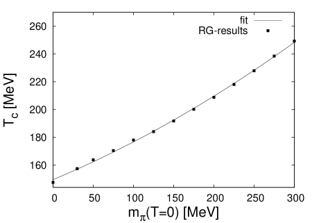
Figure 2: Chiral phase transition temperature $T_{c}$ in infinite volume as a function of $m_{\pi}(T=0)$. The dots show the result of our RG-calculation, and the line shows the result of the fit function defined in Eq. (20).

Reference	Method	$T_{c}$ [MeV]
this work	Proper-time RG	$148$
Berges (1997) Berges et al. (1999)	Functional RG, quark-meson model	$100.7$
Schaefer (1999) Schaefer and Pirner (1999)	Proper-time RG, quark-meson model	$149$
Braun (2003) Braun et al. (2004)	Proper-time RG, quark-meson model	$154$
Schaefer (2004) Schaefer and Wambach (2005)	Proper-time RG, quark-meson model	$142$
Braun (2005) Braun and Gies (2005)	Functional RG, QCD (see caption)	$186$
Gottlieb (1996) Gottlieb et al. (1997)	lattice $16^{3}\times 8$ (staggered)	$128\pm 9$
Karsch (2000) Karsch et al. (2001a)	lattice $16^{3}\times 4$ (improved staggered)	$173\pm 8$
CP-PACS (2000) Ali Khan et al. (2001)	lattice $16^{3}\times 4$ (improved Wilson)	$171\pm 4$
Bornyakov (2005) Bornyakov et al. (2005)	lattice $16^{3}\times 8$ (improved Wilson)	$173\pm 3$

Table 2: Chiral phase transition temperature in the chiral limit ($m_{\pi}\to 0$) from different RG approaches for the quark-meson model and for QCD, and from lattice simulations. We have restricted our choice of lattice references to the case of $N_{f}=2$ flavors that we have treated here. More recent lattice results have been obtained for $N_{f}=2+1$ flavors, see e.g. Karsch et al. (2001b); Fodor and Katz (2004); Bernard et al. (2005). The difference in the RG results arises from a weak dependence of $T_{c}$ on the initial values at the UV scale and on the choice of the cutoff-function Eq. (4). In Ref. Braun and Gies (2005), $T_{c}$ is calculated from a study which incorporates the running QCD coupling and all possible four-fermion interactions in the chiral symmetric regime.

IV Chiral Phase Transition Temperature in Finite Spatial Volumes

We now turn to the investigation of the chiral phase transition temperature in finite spatial volumes. As in section III, we define the phase transition temperature $T_{c}$ via the minimum of the $\sigma$-mass. Putting the system in a finite volume introduces an additional scale. Let us first discuss the influence of this additional length scale $L$ on the $\sigma$-mass and $\pi$-mass. In Fig. 3, we show the $\sigma$-mass and $\pi$-mass for $m_{\pi}^{(0)}=100\,\mathrm{{MeV}}$ and with periodic boundary conditions for the quarks, as a function of the temperature, for both a small volume $L=1\,\mathrm{{fm}}$ and a large volume $L=4\,\mathrm{{fm}}$. The minimum of the $\sigma$-mass is clearly visible in the plot. Above the transition temperature $T_{c}$, where chiral symmetry is restored, the $\sigma$- and $\pi$-mass are degenerate, independent of the size of the volume. In order to gain a better understanding of the meson masses and their dependence on the scales $L$ and $T$ in this temperature regime, we peform a perturbative one-loop calculation. Since the chiral phase is a non-perturbative phenomena, such a one-loop calculation is not trustworthy in the vicinity of the critical temperature: The extraction of the critical temperature fails, leading to an unphysical complex temperature Dolan and Jackiw (1974). Here, higher-loop terms contribute significantly, as pointed out by earlier RG flow studies, eg. Ref. Berges et al. (1999); Schaefer and Pirner (1999); Braun et al. (2004), and a study in terms of many-body resummation techniques Dumitru et al. (2004). Moreover, we neglect the quark contributions in this calculation, since they are suppressed by the appearance of a thermal Matsubara mass. In contrast, the bosonic fields have vanishing Matsubara mass and therefore their contributions dominate at high temperature. Thus our starting point for the calculation of the mass correction is the scalar $O(N=N_{f}^{2})$-model with the Lagrangian

$$\mathcal{L}=\frac{1}{2}(\partial_{\mu}\phi)^{2}+\frac{1}{2}m^{2}\phi^{2}+\frac{\lambda}{4}\phi^{4}\,,$$ (23)

where we have introduced the $O(N)$-vector $\phi=(\phi_{1},...,\phi_{N})$, and the parameters are $m=m_{UV}$ and $\lambda=\lambda_{UV}$.

The mass correction $\delta m^{2}(T,L)$, which is due to finite volume and finite temperature effects, can be decomposed into a sum of two contributions, $\delta m_{1}^{2}(T,L\!\rightarrow\!\infty)$ and $\delta m_{2}^{2}(T,L)$. We refer to Appendix B for details of the calculation.

First, in the regime defined by $0<\frac{1}{T}\ll L$, the contribution $\delta m_{1}^{2}(T,L\!\rightarrow\!\infty)$ dominates. One can estimate $\delta m_{1}^{2}(T,L\!\rightarrow\!\infty)$ for large temperatures and volumes as

$$\delta m_{1}^{2}(T,L\!\rightarrow\!\infty)\approx(N+2)\frac{\lambda}{12}T^{2}\,\;\mbox{for}\;\;T\to\infty.$$ (24)

In this case, the meson masses depend linearly on the temperature, in agreement with the result from Ref. Dolan and Jackiw (1974).

Second, if $T$ and $L$ are of the same order of magnitude, the mass correction is in essence given by

$$\delta m_{2}^{2}(T,L)\approx\frac{(N+2)\lambda}{(2\pi)^{\frac{3}{2}}}\frac{T}{L}\sum_{n=-\infty}^{\infty}\sum_{\{l_{i}\}}\!^{\prime}\Big{(}\frac{(mL)^{2}+4\pi^{2}n^{2}(TL)^{2}}{\vec{{l}}^{2}}\Big{)}^{\frac{1}{4}}K_{\frac{1}{2}}\Big{(}\sqrt{\vec{{l}}^{2}((mL)^{2}+4\pi^{2}n^{2}(TL)^{2})}\Big{)},$$ (25)

where $K_{n}$ denotes the modified Bessel-functions with index $n=\frac{1}{2}$. The vector $\vec{l}$ is defined as $\vec{{l}}=\{l_{1},l_{2},l_{3}\}$ and the prime indicates that the term with $\vec{{l}}=0$ is excluded from the summation. Note that $\delta m_{2}^{2}(T,L)$ has a complicated dependence on $T$ and $L$, but we observe that it scales with $\frac{T}{L}$, rather than with $T^{2}$. This explains the difference between the slopes of the meson masses in the regime defined by $\frac{1}{T_{c}}>\frac{1}{T}\gtrsim L$, and in the regime defined by $0<\frac{1}{T}\ll L$, which can be seen in Fig. 3.

In contrast, in the limit $TL\gg 1$ one obtains

$$\delta m_{2}^{2}(T,L)\approx\frac{3(N+2)\lambda}{\sqrt{8}\pi}\frac{T}{L}\sum_{n=-\infty}^{\infty}\sum_{\{l_{i}\}}{}^{\prime}\frac{1}{\sqrt{\vec{l}^{2}}}\exp\Big{(}-\sqrt{\vec{{l}}^{2}((mL)^{2}+4\pi^{2}n^{2}(TL)^{2})}\Big{)}.$$ (26)

The contributions from the non-vanishing thermal Matsubara-modes to $\delta m_{2}^{2}(T,L)$ drop exponentially, and $\delta m_{2}^{2}(T,L)$ becomes a linear function in the temperature $T$, due to the zeroth thermal Matsubara-mode $n=0$. Therefore, for $TL\gg 1$, $\delta m_{2}^{2}(T,L)$ is a sub-leading correction to the meson masses, compared to the contribution $\delta m_{1}^{2}(T,L)$. This describes the results for periodic quark boundary conditions well.

Similar behavior is found for anti-periodic boundary conditions of the quark fields. However, there is one essential difference between periodic and anti-periodic boundary conditions: In the case of anti-periodic boundary conditions, the quark fields have a finite minimal infrared momentum

$$p_{ap}^{\mathrm{min}}=\frac{\pi}{L}\,,$$ (27)

which is illustrated in Fig. 4. In the quark-propagator, the minimal value $p_{ap}^{\mathrm{min}}$ acts as an additional mass term which increases for decreasing volume sizes. The quark fields decouple from the RG flow as soon as the IR-cutoff scale $k$ in Eq. (11) drops below $p_{ap}^{\mathrm{min}}$. Consequently, the mesons are the only dynamical degrees of freedom in the theory for $k\leq p_{ap}^{\mathrm{min}}$: The system becomes equivalent to an $O(4)$-model, which remains in the symmetric phase for $k\rightarrow 0$.

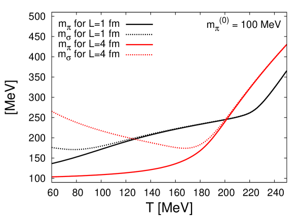
Figure 3: Sigma- and Pion-mass as functions of the temperature $T$, with $m_{\pi}^{(0)}=100\;\mathrm{MeV}$ and periodic quark boundary conditions, for $L=1\;\mathrm{{fm}}$ and $L=4\;\mathrm{{fm}}$. The solid black and the red/gray lines show the pion mass for $L=1\mathrm{{fm}}$ and $L=4\,\mathrm{{fm}}$, respectively, whereas the dotted black and red/gray lines show the sigma mass for $L=1\;\mathrm{{fm}}$ and for $L=4\;\mathrm{{fm}}$.

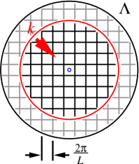
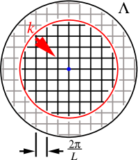
Figure 4: Schematic representation of the relation between the momentum summation and the UV- and IR-cutoff in momentum space, for anti-periodic boundary conditions (left panel) and for periodic boundary conditions (right panel). The UV-cutoff is denoted by $\Lambda$, while $k$ denotes the variable IR-cutoff of the RG scheme. The arrow indicates the direction of the RG flow from $k=\Lambda_{UV}$ to $k=0$.

Figure 5: The chiral phase transition temperature $T_{c}$ as a function of the volume size $L$, for different pion masses $m_{\pi}^{(0)}$, and for both choices of spatial quark boundary conditions. Results for periodic (anti-periodic) boundary conditions are denoted by circles (triangles), values for the pion mass at $T=0$ in infinite volume are given in the panels.

In general, the momentum scale $\frac{2\pi}{L}$ should be much smaller than the UV cut off $\Lambda_{UV}$,

$$p_{p}^{L}=\frac{2\pi}{L}\ll\Lambda_{UV}\,.$$ (28)

If $p_{p}^{L}$ becomes comparable to $\Lambda_{UV}$, there are no dynamical degrees of freedom left in our model.

We now present our main results for the volume dependence of the chiral phase transition temperature. Fig. 5 contains plots of the transition temperature $T_{c}$ as a function of the volume size, for different values of the pion mass at zero temperature, $m_{\pi}^{(0)}$, and for different choices for the quark boundary conditions. For small, realistic pion masses, $m_{\pi}^{(0)}=100\,\mathrm{MeV}$, already for $L=4\,\mathrm{{fm}}$ the results in the upper panel of Fig. 5 show a deviation of $T_{c}$ from its infinite volume value of about 6%, independent of the choice of boundary conditions. For small volume sizes $L<\frac{1}{m_{\pi}^{(0)}}$, $T_{c}$ is strongly affected by the choice of the boundary conditions for the fermions. For anti-periodic boundary conditions, we observe that $T_{c}$ decreases strongly for small volume sizes. As already discussed above, this is because of the additional infrared cutoff $p_{ap}^{\mathrm{min}}$ for the momenta of the quark fields. It is due to this additional IR-cutoff for the quarks that the system remains in the symmetric phase for small volume sizes Braun et al. (2005a, b).

For periodic quark boundary conditions, we observe a weaker volume dependence of $T_{c}$, since the condensation of the quarks is not prevented by the additional IR-cutoff $p_{ap}^{\mathrm{min}}$. For $m_{\pi}^{(0)}=100\,\mathrm{{MeV}}$ and $L\lesssim 1.5\,\mathrm{{fm}}$, we observe that $T_{c}$ is almost independent of $L$, which may be due to the fact that $p_{p}^{L}$ approaches $\Lambda_{UV}$.

For large pion masses, $m_{\pi}^{(0)}\gtrsim 300\,\mathrm{MeV}$, and for $L\geq 2\,\mathrm{{fm}}$, $T_{c}$ depends only weakly on the box size. The deviation from its infinite volume value is less than $1\%$ already for $L\approx 2.5\,\mathrm{{fm}}$. We observe only a weak dependence on the choice of the fermionic boundary conditions, as well. The reason is that the length scale set by the pion mass, $L_{\pi}\sim\frac{1}{m_{\pi}^{(0)}}$, is much smaller than the box size $L$. Therefore the volume dependence of $T_{c}$ is governed by the pion mass scale $m_{\pi}^{(0)}$, rather than the scale set by the spatial box size: pion fluctuations are more strongly suppressed by their large mass than by the long-wavelength cutoff from the finite volume. This observation implies that lattice results for $T_{c}$ are not affected by the finite volume to any considerable degree, provided the pion mass is large, $m_{\pi}^{(0)}\gtrsim 300\,\mathrm{MeV}$.

Finally, we stress that finite volumes make the coefficient $a_{1}$ in Eq. (20) bigger for smaller volumes. This can be seen from Tab. 3 and Fig. 6, where the slope of $T_{c}(m_{\pi}^{(0)},L)$ as a function of $m_{\pi}^{(0)}$ is even larger at smaller values of $L$.

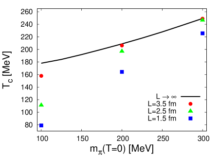
Figure 6: Chiral phase transition temperature $T_{c}$ as a function of $m_{\pi}(T=0)$ for different box sizes. We show the results for $L=1.5,\,2.5,\,3.5\;\;\mathrm{fm}$ from bottom to top. For comparison, we also show the results for infinite volume (solid line) from Fig. 2.

$L\;\mathrm{[fm]}$	$m_{\pi}^{(0)}=100\,\mathrm{{MeV}}$	$m_{\pi}^{(0)}=200\,\mathrm{{MeV}}$	$m_{\pi}^{(0)}=300\,\mathrm{{MeV}}$
$1.5$	79.0 MeV	164.3 MeV	225.7 MeV
$2.5$	111.3 MeV	197.1 MeV	246.6 MeV
$3.5$	157.9 MeV	206.3 MeV	249 MeV
$\infty$	178.1 MeV	208.3 MeV	249.3 MeV

Table 3: Chiral phase transition temperatures $T_{c}(m_{\pi}^{(0)},L)$ as function of the pion mass $m_{\pi}^{(0)}$ and the box size $L$ for periodic boundary conditions for the quark-fields. For comparison, the corresponding values in infinite spatial volume are also given.

V Conclusions

In this article, we have presented results for the volume dependence of the phase transition temperature for the chiral symmetry restoration transition. Our investigation is based on the quark-meson model and uses Renormalization Group methods. In this way, we obtain non-perturbative results for the transition temperature for various values of the pion mass.

In general, no phase transition can occur in a system of finite volume. The evaluation of lattice results therefore uses a scaling analysis in quark mass and temperature Karsch and Laermann (1994); Aoki et al. (1998); Bernard et al. (2000b); D’Elia et al. (2005), and recently finite-size scaling D’Elia et al. (2005) as an analytical tool. We expect that a Renormalization Group analysis of the critical behavior can complement these approaches.

In the present paper, we have focused on the chiral phase transition temperature, which is not universal and also model-dependent. However, the relative shift of the temperature from infinite to finite volume should depend mainly on the pion mass and the pion decay constant, which are independent of the model and represent an external input to our calculations.

We find that finite volume effects for the transition temperature remain small for large pion masses $m_{\pi}\gtrsim 300\,\mathrm{{MeV}}$, as long as the volume is of the order $L\geq 2\,\mathrm{{fm}}$ in the spatial directions. The scale for the appearance of sizable finite-volume effects is given by the pion mass $m_{\pi}$, and the effects remains small as long as $L\gg\frac{1}{m_{\pi}}$.

On the other hand, finite size effects are sizable already at a lattice extent of $L\simeq 2\,\mathrm{fm}$ for realistic pion masses of the order of $100\,\mathrm{MeV}$. We expect therefore that finite volume effects will become more relevant in future simulations with realistic pion masses. The strategy for lattice calculations should then be to simulate in volumes where the value $m_{\pi}L$ is large enough to keep the finite volume effects down to an acceptable size, and to extrapolate to smaller pion masses and the chiral limit.

We note that the choice of periodic boundary conditions in spatial directions for the quark fields, which is commonly employed in lattice simulations, leads to a much smaller finite volume effect on the transition temperature. This conclusion agrees with our results for the volume dependence of the pion mass and pion decay constant Braun et al. (2005b).

The dependence of the transition temperature on the quark mass in the quark-meson model is much stronger than that observed in lattice simulations. This must remain a puzzle in the present approach and calls for a more extensive consideration of the gluon dynamics. Work in this direction has already been started Braun and Gies (2005). In concert with other non-perturbative methods, the Renormalization Group approach should prove to be valuable as a complement to QCD lattice calculations.

Appendix A Initial Values at the UV-Scale

$m_{UV}\,\mathrm{[{MeV}]}$	$gm_{c}\,\mathrm{[{MeV}]}$	$m_{\pi}(k\rightarrow 0)\,\mathrm{[{MeV}]}$	$f_{\pi}(k\rightarrow 0)\,[\mathrm{{MeV}}]$
794	00.036	030	087
792	00.390	050	087
788	01.080	075	088
779	02.100	100	090
775	03.430	125	091
767	05.150	150	093
757	07.275	175	095
748	09.850	200	097
737	12.930	225	099
725	17.000	250	101
711	20.800	275	103
698	25.700	300	105

Table 4: Boundary conditions $a_{ij}(\Lambda_{UV})$ for the differential equations for the coefficients $a_{ij}(k)$. The corresponding values for $m_{\pi}$ and $f_{\pi}$ which result from the RG flow at zero temperature and in infinite volume are shown in the last two columns. The coefficients $a_{01}$ and $a_{02}$, which are initially non-zero, can be expressed in terms of the two parameters $m_{UV}$ and $\lambda_{UV}$, for the relation see text. As an initial condition for the flow equation for $\lambda(k)$, we have chosen $\lambda(\Lambda_{UV})=\lambda_{UV}=60$ for all parameter sets. The initial conditions for the differential equations for the remaining coefficients $a_{ij}(k)$ of the potential Eq. (18) are $a_{ij}(\Lambda_{UV})=0$. In addition, we use $g=3.258$ for the Yukawa-coupling. In our notation, $gm_{c}$ is the current quark mass.

In this section, we give an overview of the initial values for the flow equations of the coefficients $a_{ij}(k)$. As already discussed in Sec. II, we fix the values of the coefficients $a_{ij}(\Lambda_{UV})$ at the scale $\Lambda_{UV}$ in the infinite four-dimensional Euclidean volume in such a way that the values of $m_{\pi}$ and $f_{\pi}$ given by chiral perturbation Colangelo and Dürr (2004) are reproduced. However, some freedom remains in the choice of the starting values for the coefficients. But as discussed in Braun et al. (2005b), different sets of parameters give the same dependence on the size of the four dimensional volume, provided that they lead to the same values of the pion decay constant and pion mass in infinite volume. The values which we have used for our calculation can be determined from Tab. 4. In this table, we give the value for the parameter $m_{UV}$. Together with the parameter $\lambda_{UV}=\lambda(\Lambda_{UV})$ and the evolving minimum of the potential $\sigma_{0}(k)$, the two coefficients that are initially non-zero can be expressed as

$$a_{01}(\Lambda_{UV}) = \frac{1}{2}(m_{UV}^{2}+\lambda_{UV}\sigma_{0}^{2}(\Lambda_{UV}))$$ (29)

$$a_{02}(\Lambda_{UV}) = \frac{1}{4}\lambda_{UV}\,.$$ (30)

All other coefficients are initially set to zero. In principle, one should choose $\sigma_{0}(\Lambda_{UV})=0$ as initial condition, but in order to avoid numerical problems at the UV-scale, we choose a small but finite value for $\sigma_{0}$ at the UV-scale, e.g. $\sigma_{0}(\Lambda_{UV})=0.1\,\mathrm{{MeV}}$. The parameters $m_{UV}$ and $\lambda_{UV}$ can be interpreted as the usual meson masses and four-point couplings at the UV scale. The meson masses are related to the coefficients $a_{ij}$ and the minimum $\sigma_{0}$ of the potential by Braun et al. (2005a)

$$m_{\pi}^{2} = 2a_{01}$$ (31)

$$m_{\sigma}^{2} = m_{\pi}^{2}+2a_{20}+4a_{11}\sigma_{0}+8a_{02}\sigma_{0}^{2}$$ (32)

Appendix B One-Loop Calculation of the Meson Masses

In order to gain a better understanding of the slope of the meson masses as a function of temperature in the symmetric phase, we compared the RG results to a one-loop calculation for the mass of a scalar $O(N)$-model, as defined by the Lagrangian in Eq. (23). More details of the calculation are given here.

The effective potential in one-loop approximation in a $d$-dimensional Euclidean space reads

$$U^{\mathrm{{1L}}}(\phi) = \frac{1}{2}\mathrm{Tr}\log(-\partial^{2}+M^{2}(\phi))$$ (33)

$$= -\frac{1}{2}\frac{T}{L^{d-1}}\sum_{j=1}^{N}\sum_{\{n_{i}\}}\int_{\frac{1}{\Lambda^{2}}}^{\infty}\frac{ds}{s}\exp\Big{(}-s(4\pi^{2}T^{2}n_{0}^{2}+\frac{4\pi^{2}}{L^{2}}\sum_{i=1}^{d-1}n_{i}^{2}+M_{j}^{2}(\phi))\Big{)}\,,$$

where we have used Schwinger’s proper time representation of the logarithm, supplemented by a UV-cutoff $\Lambda$. In addition, we have introduced the abbreviations $M_{1}^{2}(\phi)=m^{2}+3\lambda\phi^{2}$ and $M_{j}^{2}(\phi)=m^{2}+\lambda\phi^{2}$ for $j=2,...,N$. The sum runs over all permutations of $\{n_{1},...,n_{d}\}$. Here $L$ denotes the length of the $d$-dimensional box in space directions, and $\frac{1}{T}$ denotes the length of the box in the Euclidean time direction. In order to calculate the mass of the scalar field, we use the Jacobi-Elliptic-Theta function $\vartheta_{p}(s)$, defined in Eq. (16). Both representations of this function given in Eq. (16) deserve some comments: The first representation in Eq. (16) is essentially the usual Matsubara summation, where a truncation of the Matsubara sum can be used to perform a high-temperature or small-volume expansion of the one-loop effective potential. In order to get the second representation in Eq. (16), we have applied Poisson’s formula to the first representation. This second representation allows to separate the UV divergence of the effective potential: the divergent infinite-volume contribution, which is given by the first term of the left-hand side of Eq. (16), can be separated from the volume and temperature dependent parts. In addition, a truncation of the sum in the second representation can be used to perform a low-temperature or large-volume expansion of the one-loop effective potential.

With the second representation of the Jacobi-Elliptic-Theta function from Eq. (16), we can divide the one-loop effective potential in three contributions,

$$U^{\mathrm{{1L}}}=U_{\infty}^{\mathrm{{1L}}}(T\!\rightarrow\!0,L\!\rightarrow\!\infty)+U_{1}^{\mathrm{{1L}}}(T,L\!\rightarrow\!\infty)+U_{2}^{\mathrm{{1L}}}(T,L)\,.$$ (34)

We do not consider the contribution $U_{\infty}^{\mathrm{{1L}}}$ in the following, since we are only interested in the finite-temperature and finite-volume corrections to the mass. We start with the calculation of the mass correction due to the volume-independent contribution $U_{1}^{\mathrm{{1L}}}(T)=U_{1}^{\mathrm{{1L}}}(T,L\!\rightarrow\!\infty)$ which is given by

$$U_{1}^{\mathrm{{1L}}}(T)=-\frac{1}{(4\pi)^{\frac{d}{2}}}\sum_{j=1}^{N}\sum_{q=1}^{\infty}\int_{0}^{\infty}\frac{ds}{s^{1+\frac{d}{2}}}\exp\Big{(}-\frac{q^{2}}{4sT^{2}}-sM_{j}^{2}(\phi)\Big{)}\,.$$ (35)

We stress that the regulator $\Lambda$ of the Schwinger proper-time integral can be removed here, $\Lambda\rightarrow\infty$. In order to calculate the mass correction in the symmetric phase, we have to take the second derivative of $U_{1}^{\mathrm{{1L}}}(T)$ with respect to the field $\phi$ and evaluate the resulting expression at $\phi=0$:

$$\delta m_{1}^{2}(T)=\left.\frac{\partial^{2}}{\partial\phi^{2}}U_{1}^{\mathrm{{1L}}}(T)\right|_{\phi=0}=\frac{2(N+2)\lambda}{(2\pi)^{\frac{d}{2}}}(mT)^{\frac{d-2}{2}}\sum_{q=1}^{\infty}\frac{1}{q^{\frac{d-2}{2}}}\,K_{\frac{d-2}{2}}\big{(}\frac{qm}{T}\big{)}\,.$$ (36)

Now we make use of the integral representation of the modified Bessel Functions,

$$2\left(\frac{x}{2}\right)^{\nu}K_{\nu}(x)=\int_{{}_{0}}^{\infty}dss^{\nu-1}\mathrm{e}^{-s-\frac{\pi^{2}}{4s}}\,.$$ (37)

For $T\rightarrow\infty$ and $d=4$, we use

$$K_{1}(x)\approx\frac{1}{x}\quad(x\ll 1)\,,$$ (38)

and obtain the simple expression

$$\delta m_{1}^{2}(T)\approx\frac{(N+2)\lambda}{12}T^{2}$$ (39)

for the correction $\delta m_{1}^{2}(T)$, which agrees with the result found in Dolan and Jackiw (1974).

Now we turn to the calculation of the mass correction due to the contribution $U_{2}^{\mathrm{{1L}}}(T,L)$. Since we are interested in small spatial volumes and high temperatures, we use the Poisson-representation for the spatial contributions, but we still use the usual Matsubara sum for the thermal contribution. The contribution $U_{2}^{\mathrm{{1L}}}(T,L)$ to the potential is

$$U_{2}^{\mathrm{{1L}}}(T,L)=-\frac{T}{2(4\pi)^{\frac{d-1}{2}}}\sum_{j=1}^{N}\sum_{n=-\infty}^{\infty}\sum_{\{l_{i}\}}\!^{\prime}\int_{0}^{\infty}\frac{ds}{s^{1+\frac{d-1}{2}}}\exp\Big{(}-s(M_{j}^{2}(\phi)+4\pi^{2}n^{2}T^{2})-\frac{\vec{{l}}^{2}L^{2}}{4s}\Big{)}\,.$$ (40)

The vector $\vec{l}$ is defined as $\vec{{l}}=\{l_{1},l_{2},l_{3}\}$, and the prime indicates that the term with $\vec{{l}}=0$ is excluded from the summation. The regulator $\Lambda$ can also be removed here. Taking the second derivative with respect to the fields $\phi$ and evaluating at $\phi=0$, we obtain the corresponding mass correction

$$\delta m_{2}^{2}(T,L) =\left.\frac{\partial^{2}}{\partial\phi^{2}}U_{2}^{\mathrm{{1L}}}(T,L)\right|_{\phi=0}$$

$$=\frac{(N+2)\lambda TL^{-\frac{d-3}{2}}}{(2\pi)^{\frac{d-1}{2}}}\sum_{n=-\infty}^{\infty}\sum_{\{l_{i}\}}\!^{\prime}\Big{(}\frac{m^{2}+4\pi^{2}n^{2}T^{2}}{\vec{{l}}^{2}}\Big{)}^{\frac{d-3}{4}}K_{\frac{d-3}{2}}\Big{(}\sqrt{\vec{{l}}^{2}((mL)^{2}+4\pi^{2}n^{2}(TL)^{2})}\Big{)}\,.$$

We used again the integral representation of the modified Bessel functions Eq. (37). Finally, we show that this contribution becomes proportional to the temperature $\frac{T}{L}$ for $TL\gg 1$. For this purpose, we use the asymptotic expansion of the Bessel-functions for large arguments, given by

$$K_{\nu}(x)\approx\sqrt{\frac{\pi}{x}}\mathrm{e}^{-x}\quad(x\gg 1)\,.$$ (42)

Using Eq. (42), the mass correction $\delta m_{2}^{2}(T,L)$ for $TL\gg 1$ and $d=4$ reads

$$\delta m_{2}^{2}(T,L)\approx\frac{3(N+2)\lambda}{8^{\frac{1}{2}}\pi}\frac{T}{L}\sum_{n=-\infty}^{\infty}\sum_{\{l_{i}\}}\!^{\prime}\frac{1}{\sqrt{\vec{{l}}^{2}}}\exp\left(-\sqrt{\vec{{l}}^{2}\left((mL)^{2}+4\pi^{2}n^{2}(TL)^{2}\right)}\right),$$ (43)

which drops exponentially in the limit $TL\rightarrow\infty$ for non-vanishing thermal Matsubara-modes, whereas the contribution from the zeroth thermal Matsubara-mode ($n=0$) remains finite and is proportional to the temperature $T$. For $TL\gg 1$, the mass-correction $\delta m_{2}^{2}(T,L)$ is therefore sub-leading, compared to the contribution $\delta m_{1}^{2}(T)$.

References

- Fodor and Katz (2002) Z. Fodor and S. D. Katz, JHEP 03, 014 (2002), eprint hep-lat/0106002.
- Fodor and Katz (2004) Z. Fodor and S. D. Katz, JHEP 04, 050 (2004), eprint hep-lat/0402006.
- Allton et al. (2002) C. R. Allton et al., Phys. Rev. D66, 074507 (2002), eprint hep-lat/0204010.
- Allton et al. (2003) C. R. Allton et al., Phys. Rev. D68, 014507 (2003), eprint hep-lat/0305007.
- Philipsen (2005) O. Philipsen (2005), eprint hep-lat/0510077.
- de Forcrand and Philipsen (2002) P. de Forcrand and O. Philipsen, Nucl. Phys. B642, 290 (2002), eprint hep-lat/0205016.
- de Forcrand and Philipsen (2003) P. de Forcrand and O. Philipsen, Nucl. Phys. B673, 170 (2003), eprint hep-lat/0307020.
- Schaefer and Wambach (2005) B.-J. Schaefer and J. Wambach, Nucl. Phys. A757, 479 (2005), eprint nucl-th/0403039.
- Gavai and Gupta (2005) R. V. Gavai and S. Gupta, Phys. Rev. D71, 114014 (2005), eprint hep-lat/0412035.
- Allton et al. (2005) C. R. Allton et al., Phys. Rev. D71, 054508 (2005), eprint hep-lat/0501030.
- Pisarski and Wilczek (1984) R. D. Pisarski and F. Wilczek, Phys. Rev. D29, 338 (1984).
- D’Elia et al. (2005) M. D’Elia, A. Di Giacomo, and C. Pica (2005), eprint hep-lat/0503030.
- Karsch et al. (2001a) F. Karsch, E. Laermann, and A. Peikert, Nucl. Phys. B605, 579 (2001a), eprint hep-lat/0012023.
- Karsch et al. (2001b) F. Karsch, E. Laermann, and C. Schmidt, Phys. Lett. B520, 41 (2001b), eprint hep-lat/0107020.
- Weinberg (1979) S. Weinberg, Physica A96, 327 (1979).
- Gasser and Leutwyler (1984) J. Gasser and H. Leutwyler, Ann. Phys. 158, 142 (1984).
- Gasser and Leutwyler (1985) J. Gasser and H. Leutwyler, Nucl. Phys. B250, 465 (1985).
- Farchioni et al. (2003) F. Farchioni, I. Montvay, E. Scholz, and L. Scorzato (qq+q), Eur. Phys. J. C31, 227 (2003), eprint hep-lat/0307002.
- Farchioni et al. (2005) F. Farchioni et al., Eur. Phys. J. C42, 73 (2005), eprint hep-lat/0410031.
- Chen et al. (2001) P. Chen et al., Phys. Rev. D64, 014503 (2001), eprint hep-lat/0006010.
- Aoki et al. (2004) Y. Aoki et al. (2004), eprint hep-lat/0411006.
- Colangelo et al. (2003) G. Colangelo, S. Dürr, and R. Sommer, Nucl. Phys. Proc. Suppl. 119, 254 (2003), eprint hep-lat/0209110.
- Colangelo and Dürr (2004) G. Colangelo and S. Dürr, Eur. Phys. J. C33, 543 (2004), eprint hep-lat/0311023.
- Colangelo et al. (2005) G. Colangelo, S. Dürr, and C. Haefeli, Nucl. Phys. B721, 136 (2005), eprint hep-lat/0503014.
- Braun et al. (2005a) J. Braun, B. Klein, and H. J. Pirner, Phys. Rev. D71, 014032 (2005a), eprint hep-ph/0408116.
- Braun et al. (2005b) J. Braun, B. Klein, and H. J. Pirner, Phys. Rev. D72, 034017 (2005b), eprint hep-ph/0504127.
- Fischer and Alkofer (2002) C. S. Fischer and R. Alkofer, Phys. Lett. B536, 177 (2002), eprint hep-ph/0202202.
- Maas et al. (2004) A. Maas, J. Wambach, B. Gruter, and R. Alkofer, Eur. Phys. J. C37, 335 (2004), eprint hep-ph/0408074.
- Maas et al. (2005) A. Maas, J. Wambach, and R. Alkofer, Eur. Phys. J. C42, 93 (2005), eprint hep-ph/0504019.
- Maas (2005) A. Maas, Mod. Phys. Lett. A20, 1797 (2005), eprint hep-ph/0506066.
- Fischer and Pennington (2005) C. S. Fischer and M. R. Pennington (2005), eprint hep-ph/0512233.
- Pawlowski et al. (2004) J. M. Pawlowski, D. F. Litim, S. Nedelko, and L. von Smekal, Phys. Rev. Lett. 93, 152002 (2004), eprint hep-th/0312324.
- Gies (2002) H. Gies, Phys. Rev. D66, 025006 (2002), eprint hep-th/0202207.
- Fischer and Gies (2004) C. S. Fischer and H. Gies, JHEP 10, 048 (2004), eprint hep-ph/0408089.
- Gies and Jaeckel (2005) H. Gies and J. Jaeckel (2005), eprint hep-ph/0507171.
- Braun and Gies (2005) J. Braun and H. Gies (2005), eprint hep-ph/0512085.
- Nambu and Jona-Lasinio (1961) Y. Nambu and G. Jona-Lasinio, Phys. Rev. 122, 345 (1961).
- Bijnens (1996) J. Bijnens, Phys. Rept. 265, 369 (1996), eprint hep-ph/9502335.
- Berges et al. (1999) J. Berges, D. U. Jungnickel, and C. Wetterich, Phys. Rev. D59, 034010 (1999), eprint hep-ph/9705474.
- Ratti et al. (2005) C. Ratti, M. A. Thaler, and W. Weise (2005), eprint hep-ph/0506234.
- Wilson and Kogut (1974) K. G. Wilson and J. B. Kogut, Phys. Rept. 12, 75 (1974).
- Wegner and Houghton (1973) F. J. Wegner and A. Houghton, Phys. Rev. A8, 401 (1973).
- Wetterich (1993) C. Wetterich, Phys. Lett. B301, 90 (1993).
- Liao (1996) S.-B. Liao, Phys. Rev. D53, 2020 (1996), eprint hep-th/9501124.
- Schaefer and Pirner (1999) B.-J. Schaefer and H.-J. Pirner, Nucl. Phys. A660, 439 (1999), eprint nucl-th/9903003.
- Goldenfeld (1992) N. Goldenfeld (1992), reading, USA: Addison-Wesley (1992) 394 p. (Frontiers in physics, 85).
- Karsch and Laermann (1994) F. Karsch and E. Laermann, Phys. Rev. D50, 6954 (1994), eprint hep-lat/9406008.
- Aoki et al. (1998) S. Aoki et al. (JLQCD), Phys. Rev. D57, 3910 (1998), eprint hep-lat/9710048.
- Bernard et al. (2000a) C. W. Bernard et al., Phys. Rev. D61, 054503 (2000a), eprint hep-lat/9908008.
- Asakawa and Yazaki (1989) M. Asakawa and K. Yazaki, Nucl. Phys. A504, 668 (1989).
- Lutz et al. (1992) M. Lutz, S. Klimt, and W. Weise, Nucl. Phys. A542, 521 (1992).
- Boyd et al. (1994) G. Boyd, S. Gupta, F. Karsch, and E. Laermann, Z. Phys. C64, 331 (1994), eprint hep-lat/9405006.
- Rezaeian and Pirner (2005) A. H. Rezaeian and H.-J. Pirner (2005), eprint nucl-th/0510041.
- Rezaeian (2005) A. H. Rezaeian (2005), eprint nucl-th/0512027.
- Klevansky (1992) S. P. Klevansky, Rev. Mod. Phys. 64, 649 (1992).
- Bernard et al. (2005) C. Bernard et al. (MILC), Phys. Rev. D71, 034504 (2005), eprint hep-lat/0405029.
- Braun et al. (2004) J. Braun, K. Schwenzer, and H.-J. Pirner, Phys. Rev. D70, 085016 (2004), eprint hep-ph/0312277.
- Gottlieb et al. (1997) S. A. Gottlieb et al., Phys. Rev. D55, 6852 (1997), eprint hep-lat/9612020.
- Ali Khan et al. (2001) A. Ali Khan et al. (CP-PACS), Phys. Rev. D63, 034502 (2001), eprint hep-lat/0008011.
- Bornyakov et al. (2005) V. G. Bornyakov et al., Proc. Sci. LAT2005, 157 (2005), eprint hep-lat/0509122.
- Dolan and Jackiw (1974) L. Dolan and R. Jackiw, Phys. Rev. D9, 3320 (1974).
- Dumitru et al. (2004) A. Dumitru, D. Roder, and J. Ruppert, Phys. Rev. D70, 074001 (2004), eprint hep-ph/0311119.
- Bernard et al. (2000b) C. W. Bernard et al. (MILC), Phys. Rev. D61, 111502 (2000b), eprint hep-lat/9912018.