Improved Measurement of $ttZ$ Couplings at the LHC

Abstract

We consider QCD $t\bar{t}Z$ production at the LHC with $Z\to\bar{\nu}\nu$ and all-hadronic $t\bar{t}$ decays, i.e. $pp\to p\hbox to0.0pt{\hss/}_{T}b\bar{b}$+4 jets, as a tool to measure $ttZ$ couplings. This channel has a significantly larger cross section than those where the $Z$ boson decays leptonically. However, $t\bar{t}$, $b\bar{b}+4$ jet, $t\bar{t}j$ and $t\bar{t}jj$ production give rise to potentially large backgrounds. We show that these processes can be suppressed to an acceptable level with suitable cuts, and find that adding the $p\hbox to0.0pt{\hss/}_{T}b\bar{b}+4$ jet channel to the final states used in previous $ttZ$ couplings analyses will improve the sensitivity by $10-60\%$. We also discuss how the measurement of the $ttZ$ couplings may constrain Little Higgs models.

I Introduction

Although the top quark was discovered more than ten years ago topcdf ; topd0 , many of its properties are still only poorly known Chakraborty:2003iw . In particular, the couplings of the top quark to the electroweak (EW) gauge bosons have not yet been directly measured.  The large top quark mass PDF2005 suggests that it may play a special role in EW symmetry breaking (EWSB). New physics connected with EWSB may thus be found first in top quark precision observables. A possible signal for new physics is a deviation of the any of the $tt\gamma$, $ttZ$ or $tbW$ couplings from the values predicted by the Standard Model (SM). For example, in technicolor and other models with a strongly coupled Higgs sector examples , and in Little Higgs models Berger:2005ht , anomalous top quark couplings may be induced at the $5-10\%$ level.

Current data provide only weak constraints on the top quark couplings to EW gauge bosons, except for the $ttZ$ vector and axial vector couplings, which are rather tightly but indirectly constrained by LEP/SLC $Z$-pole data (see Ref. Baur:2004uw and references therein); and the right-handed $tbW$ coupling, which is severely bounded by the observed $b\to s\gamma$ rate Larios:1999au . Future collider experiments offer many possibilities to probe the EW top quark couplings. The most promising ones with respect to the $ttV$ ($V=\gamma,\,Z$) couplings are provided by an $e^{+}e^{-}$ linear collider via $e^{+}e^{-}\to\gamma^{*}/Z^{*}\to t\bar{t}$ Grzadkowski:1998bh ; Grzadkowski:2000nx ; Lin:2001yq ; Abe:2001nq ; Aguilar-Saavedra:2001rg ; Frey:1995ai ; Ladinsky:1992vv , and the LHC via $t\bar{t}V$ production Baur:2004uw ; Zhou:1998bh ; Baur:2001si .

At an $e^{+}e^{-}$ linear collider operating at $\sqrt{s}=500$ GeV and with an integrated luminosity of $100-200$ fb^-1, one could measure the $ttV$ couplings in top pair production with a few-percent precision Abe:2001nq . However, the process $e^{+}e^{-}\to\gamma^{*}/Z^{*}\to t\bar{t}$ is sensitive to both $tt\gamma$ and $ttZ$ couplings simultaneously, and significant cancellations between the various couplings can occur. At hadron colliders, $t\bar{t}$ production is so dominated by the QCD processes $gg,q\bar{q}\to t\bar{t}$ that a measurement of the EW neutral couplings via $q\bar{q}\to\gamma^{*}/Z^{*}\to t\bar{t}$ is hopeless. Instead, they can be measured in QCD $t\bar{t}Z/\gamma$ production and radiative top quark decays in $t\bar{t}$ events ($t\bar{t}\to\gamma W^{+}W^{-}b\bar{b}$). Each of the processes is sensitive to the EW couplings of only the boson emitted: $Z$ and photon independently. This obviates having to disentangle potential cancellations between the different couplings. In these three processes one can also hope to separate the dimension-four and -five couplings which appear in the effective Lagrangian describing $ttV$ interactions.

In Ref. Baur:2004uw we presented a detailed analysis of $t\bar{t}V$ production at hadron colliders. We found that while the $tt\gamma$ couplings can be measured at the LHC with a precision of typically a few percent, the bounds on the $ttZ$ couplings are a factor $3-10$ weaker, in particular for the vector and axial vector couplings, $F_{1V}^{Z}$ and $F_{1A}^{Z}$. A major factor which limits their sensitivity is the relatively small cross section for $t\bar{t}Z$ production when one requires the $Z$ boson to decay leptonically (where we mean $\ell^{+}\ell^{-}$ ($\ell=e,\mu$) throughout), as in our previous analysis.

In this paper, we extend our $t\bar{t}Z$ analysis to the case where the $t\bar{t}$ pair decays hadronically and the $Z$ boson decays into neutrinos. Due to the larger branching ratio for $Z\to\bar{\nu}\nu$ relative to leptonic decays, this effectively triples the number of events which can be utilized, thus our present analysis may significantly improve the limits on anomalous $ttZ$ couplings. However, the increased statistics comes at the price of a background which is potentially much larger than the signal. After reviewing the definition of the $ttZ$ couplings, we present a detailed discussion of the signal and all relevant backgrounds (Sec. II), showing that the most important backgrounds can be adequately suppressed by imposing suitable cuts. In Sec. III we derive sensitivity bounds for the $b\bar{b}\bar{\nu}\nu$+$4j$ final state and combine them with those we obtained previously Baur:2004uw . We also explore how a $ttZ$ coupling measurement at the LHC may help constrain parameters of Little Higgs models. We summarize our findings in Sec. IV.

II Calculation of Signal and Background

II.1 Definition of general $ttZ$ couplings

The most general Lorentz-invariant vertex function describing the interaction of a $Z$ boson with two top quarks can be written in terms of ten form factors Hollik:1998vz , which are functions of the kinematic invariants. In the low energy limit, these correspond to couplings which multiply dimension-four or -five operators in an effective Lagrangian, and may be complex. If the $Z$ boson couples to effectively massless fermions, the number of independent form factors is reduced to eight. In addition, if both top quarks are on-shell, the number is further reduced to four. In this case, the $ttZ$ vertex can be written in the form

$$\Gamma_{\mu}^{ttZ}(k^{2},\,q,\,\bar{q})=-ie\left\{\gamma_{\mu}\,\left(F_{1V}^{Z}(k^{2})+\gamma_{5}F_{1A}^{Z}(k^{2})\right)+\frac{\sigma_{\mu\nu}}{2m_{t}}~{}(q+\bar{q})^{\nu}\left(iF_{2V}^{Z}(k^{2})+\gamma_{5}F_{2A}^{Z}(k^{2})\right)\right\}\,,$$ (1)

where $e$ is the proton charge, $m_{t}$ is the top quark mass, $q~{}(\bar{q})$ is the outgoing top (anti-top) quark four-momentum, and $k^{2}=(q+\bar{q})^{2}$. The terms $F_{1V}^{Z}(0)$ and $F_{1A}^{Z}(0)$ in the low energy limit are the $ttZ$ vector and axial vector form factors. The coefficients $F_{2V}^{Z}(M_{Z}^{2})$ and $F_{2A}^{Z}(M_{Z}^{2})$, where $M_{Z}$ is the $Z$ boson mass, are related to the the weak magnetic and ($CP$-violating) weak electric dipole moments, $g_{t}^{Z}$ and $d_{t}^{Z}$. At tree level in the SM,

$$F^{Z,SM}_{1V} =-\frac{1}{4\sin\theta_{W}\cos\theta_{W}}\left(1-\frac{8}{3}\,\sin^{2}\theta_{W}\right), \qquad F^{Z,SM}_{1A} =\frac{1}{4\sin\theta_{W}\cos\theta_{W}}\,,$$

$$F^{Z,SM}_{2V} =0\,, \qquad F^{Z,SM}_{2A} =0\,,$$

where $\theta_{W}$ is the weak mixing angle. The numerically most important radiative corrections to the vector and axial vector couplings can be taken into account by replacing the factor $(1-8\sin^{2}\theta_{W}/3)$ in $F^{Z,SM}_{1V}$ by $(1-8\sin^{2}\theta_{eff}^{t}/3)$, where $\sin^{2}\theta_{eff}^{t}$ is the effective mixing angle; and by expressing the remaining factors of $\sin\theta_{W}$ and $\cos\theta_{W}$ in $F^{Z,SM}_{1V,A}$ in terms of the physical $W$ and $Z$ masses. Numerically, the one-loop corrections to $F^{Z}_{1V,A}$ are typically of ${\cal O}(10^{-2}-10^{-3})$ Hollik:1988ii . The weak magnetic dipole form factor $F^{Z}_{2V}$ receives contributions of the same magnitude Bernabeu:1995gs at the one-loop level in the SM. However, there is no such contribution to the weak electric dipole form factors, $F^{Z}_{2A}$ Hollik:1998vz .

$S$-matrix unitarity restricts $\Delta F^{Z}_{1V,A}(0)=F^{Z}_{1V,A}(0)-F^{Z,SM}_{1V,A}$ to be $\lesssim{\cal O}(1)$ if the scale of new physics is of the order of a few TeV Baur:2004uw ; Hosch:1996wu .

II.2 Signal

The process $pp\to t\bar{t}Z$ with leptonic $Z$ boson decay was considered in detail in Ref. Baur:2004uw . Here we concentrate on final states where $Z\to\bar{\nu}\nu$. Since the $t\bar{t}Z$ cross section is too small to be observable at the Tevatron, we concentrate our efforts on the LHC. The neutrinos escape undetected and, thus, manifest themselves in the form of missing transverse momentum, $p\hbox to0.0pt{\hss/}_{T}$. If one or both $W$ bosons originating from the top decay, $t\to Wb$, decay leptonically, the observed states, $\ell p\hbox to0.0pt{\hss/}_{T}b\bar{b}jj$ and $\ell\ell^{\prime}p\hbox to0.0pt{\hss/}_{T}b\bar{b}$, are identical to those resulting from ordinary $t\bar{t}$ production. As the $t\bar{t}$ cross section is more than a factor 1000 larger than that of $t\bar{t}Z$, it will be very difficult to sufficiently suppress this background. We therefore consider only the case where both $W$ bosons decay hadronically,

$$pp\to p\hbox to0.0pt{\hss/}_{T}b\bar{b}+4j\,.$$ (2)

We assume that both $b$ quarks are tagged with a combined efficiency of $\epsilon_{b}^{2}=0.4$. Note that, since there is essentially no phase space for $t\to WZb$ decays ($BR(t\to WZb)\approx 3\cdot 10^{-6}$ Mahlon:1994us ; Altarelli:2000nt ), $t\bar{t}$ production with one top decaying into $WZb$ does not contribute to the final state of Eq. (2).

We perform our calculation for general $ttZ$ couplings of the form of Eq. (1). At LHC energies, $Z$ boson transverse momenta of at most a few hundred GeV are accessible in $t\bar{t}Z$ production. The scale of new physics responsible for anomalous $ttZ$ couplings would be expected to be of ${\cal O}(1$ TeV) or higher. Form factor effects will thus be small and are therefore neglected in the following. We also assume that all $ttZ$ couplings are real. We otherwise assume the SM to be valid. Our calculation includes top quark and $Z$ boson decays with full spin correlations and finite width effects. All top quark resonant Feynman diagrams are included. To ensure gauge invariance of the SM result, we use the so-called overall-factor scheme of Ref. Baur:1991pp as implemented in the madgraph Stelzer:1994ta -derived code of Ref. Maltoni:2002jr .

All signal and background cross sections in this paper are computed using CTEQ6L1 Pumplin:2002vw parton distribution functions with the strong coupling constant evaluated at leading order and $\alpha_{s}(M_{Z}^{2})=0.130$. We set the top quark mass to $m_{t}=178$ GeV topmass . All signal cross sections in this paper are calculated for factorization and renormalization scales equal to $m_{t}$.

The basic acceptance cuts for $p\hbox to0.0pt{\hss/}_{T}b\bar{b}$+$4j$ events at the LHC are

$$p_{T}(b)>20~{}{\rm GeV}\;,\qquad|\eta(b)|<2.5\;,\qquad\Delta R(b,b)>0.4\;,$$

$$p_{T}(j)>30~{}{\rm GeV}\;,\qquad|\eta(j)|<2.5\;,\qquad\Delta R(j,j)>0.4\;,\qquad\Delta R(j,b)>0.4\;,$$ (3)

where $\Delta R=[(\Delta\phi)^{2}+(\Delta\eta)^{2}]^{1/2}$ is the separation in pseudorapidity–azimuth space. We include minimal detector effects via Gaussian smearing of parton momenta according to CMS cms expectations, and take into account the $b$ jet energy loss via a parameterized function. To ensure that the LHC experiments can trigger on the events of interest, we require at least three ($b$- or non-$b$) jets to have

$$p_{T}(j)>50~{}{\rm GeV}$$ (4)

and

$$p\hbox to0.0pt{\hss/}_{T}>5~{}{\rm GeV}^{1/2}\sqrt{\sum p_{T}}\,,$$ (5)

where the sum extends over jets and $b$ quarks in the final state. Furthermore, to reduce the background from non-resonant $Zb\bar{b}+4j$ production and singly-resonant processes such as $pp\to t\bar{b}Zjj$, we require that the two $b$ quarks and four jets are consistent with originating from a $t\bar{t}$ pair. This is accomplished by selecting events which satisfy

$$\chi^{2}_{min}=\min_{b_{1}j_{1}j_{2}b_{2}j_{3}j_{4}~{}perm}\left[\chi^{2}(b_{1}j_{1}j_{2};b_{2}j_{3}j_{4})\right]<3$$ (6)

where $\chi^{2}_{min}$ is the minimum of the $\chi^{2}(b_{1}j_{1}j_{2};b_{2}j_{3}j_{4})$ values of all possible combinations of jet pairs and $bjj$ combinations, and

$$\chi^{2}(b_{1}j_{1}j_{2};b_{2}j_{3}j_{4}) = \frac{(m(j_{1}j_{2})-M_{W})^{2}}{\sigma_{W}^{2}}+\frac{(m(j_{3}j_{4})-M_{W})^{2}}{\sigma_{W}^{2}}+$$

$$\frac{(m(b_{1}j_{1}j_{2})-m_{t})^{2}}{\sigma_{t}^{2}}+\frac{(m(b_{2}j_{3}j_{4})-m_{t})^{2}}{\sigma_{t}^{2}}\;.$$

For the $W\to jj$ and $t\to bjj$ invariant mass resolutions we take $\sigma_{W}=7.8$ GeV and $\sigma_{t}=13.4$ GeV Beneke:2000hk .

As we discuss in more detail below, potentially large backgrounds arise from ordinary $t\bar{t}$ and $b\bar{b}$+$4j$ production where the four momentum vector of one or more jets is badly mismeasured. In contrast to signal events, the azimuthal opening angle $\Delta\phi(p\hbox to0.0pt{\hss/}_{T},p_{T}(b\bar{b}))$ between the missing transverse momentum and the transverse momentum of the two $b$ quarks,

$${\mathbf{p}}_{T}(b\bar{b})={\mathbf{p}}_{T}(b)+{\mathbf{p}}_{T}(b)$$ (8)

in $t\bar{t}$ and $b\bar{b}+4j$ background events is typically smaller than $90^{\circ}$. The same is also true for the azimuthal opening angle $\Delta\phi(p\hbox to0.0pt{\hss/}_{T},p_{T}(had))$ between the missing transverse momentum and the transverse momentum of the four leading non-$b$ jets,

$${\mathbf{p}}_{T}(had)=\sum_{i=1}^{4}{\mathbf{p}}_{T}(j_{i}).$$ (9)

In addition to the cuts listed in Eqs. (II.2)– (6), we therefore require

$$\Delta\phi(p\hbox to0.0pt{\hss/}_{T},p_{T}(b\bar{b}))>100^{\circ},\qquad\Delta\phi(p\hbox to0.0pt{\hss/}_{T},p_{T}(had))>100^{\circ}~{}.$$ (10)

Imposing the cuts listed in Eqs. (II.2)– (10), and before taking into account $b$-tagging efficiencies, we obtain a signal cross section of about 3.4 fb.

II.3 Background processes

The potentially most dangerous irreducible background to $p\hbox to0.0pt{\hss/}_{T}b\bar{b}$+$4j$ production originates from $t\bar{t}j$ production, where one top quark decays hadronically, $t\to Wb\to bjj$, and the other via $t\to Wb\to\tau\nu_{\tau}b$ with the $\tau$-lepton decaying hadronically, $\tau\to h\nu_{\tau}$. We calculate this process using tree level matrix elements which include all decay correlations. Because of its small mass and typically high transverse momentum, we simulate $\tau$ decays in the collinear approximation. All $\tau$ decays are calculated following the approach described in Ref. wbf_ll . For the probability that a $\tau$-jet is misidentified as a light quark/gluon jet we assume a constant value of $P_{h\to j}=20\%$. Ref. tauveto found that $P_{h\to j}$ decreases with increasing jet transverse momentum, from $20\%$ for $p_{T}(j)=20$ GeV to $5\%$ at $p_{T}(j)=60$ GeV. Our results for the $t\bar{t}j$ background thus should be regarded as conservative.

Other contributions to the irreducible background arise from singly-resonant top quark production ($t\bar{b}Zjj$ and $\bar{t}bZjj$), and from non-resonant $WZb\bar{b}jj$ and $Zb\bar{b}+4j$ production. The calculation of these backgrounds was discussed in detail in Ref. Baur:2004uw for $Z\to\ell^{+}\ell^{-}$ decays. It is straightforward to adapt the calculation to $Z\to\bar{\nu}\nu$ decays. Finally, $t\bar{t}jj$ production with $t\bar{t}\to\tau^{+}\nu_{\tau}\tau^{-}\bar{\nu}_{\tau}b\bar{b}$ and both $\tau$-leptons decaying hadronically has to be considered. We calculate this background using alpgen Mangano:2002ea , treating $\tau$ decays the same as for the $t\bar{t}j$ background discussed above.

There are also several reducible backgrounds which result from missing transverse momentum arising from badly-mismeasured jet momenta, or from not detecting a charged lepton. The main contributions to the first category arise from $t\bar{t}$, $b\bar{b}$+$4j$ and $6j$ production. We calculate the latter two processes using alpgen. QCD $6j$ production contributes only if two light jets are misidentified as $b$ jets. To estimate the contribution of this process we assume the probability for a light jet to be misidentified as a $b$ jet to be $P_{j\to b}=1/100$. QCD $t\bar{t}jj$ production contributes to the background if $t\bar{t}\to\ell^{\pm}\nu_{\ell}b\bar{b}jj$ ($\ell=e,\,\mu$) and the charged lepton is missed. Likewise, $pp\to t\bar{t}W$ contributes if the $t\bar{t}$ system decays hadronically, $t\bar{t}\to b\bar{b}$+$4j$, and the lepton in $W\to\ell\nu$ is missed; or if $t\bar{t}\to\ell^{\pm}\nu_{\ell}b\bar{b}jj$ and $W\to jj$. We assume that an electron or muon is missed if $|\eta(\ell)|>2.5$, $p_{T}(\ell)<10$ GeV, or if either $\Delta R(\ell,j)<0.4$ or $\Delta R(\ell,b)<0.4$. Since electrons can be detected, albeit with reduced efficiency, at rapidities larger than 2.5 using the forward electromagnetic calorimeter, our estimates of the $t\bar{t}jj$ and $t\bar{t}W$ backgrounds are conservative. We calculate the $t\bar{t}jj$ background again using alpgen.

Our calculation of the $t\bar{t}j(j)$ backgrounds does not include contributions from $t\bar{t}(j)$ production where one or both top quarks decay radiatively, $t\to Wbj(j)$. Due to the $p\hbox to0.0pt{\hss/}_{T}$ and $\chi^{2}$ cuts of Eqs. (5) and (6), such contributions are strongly suppressed.

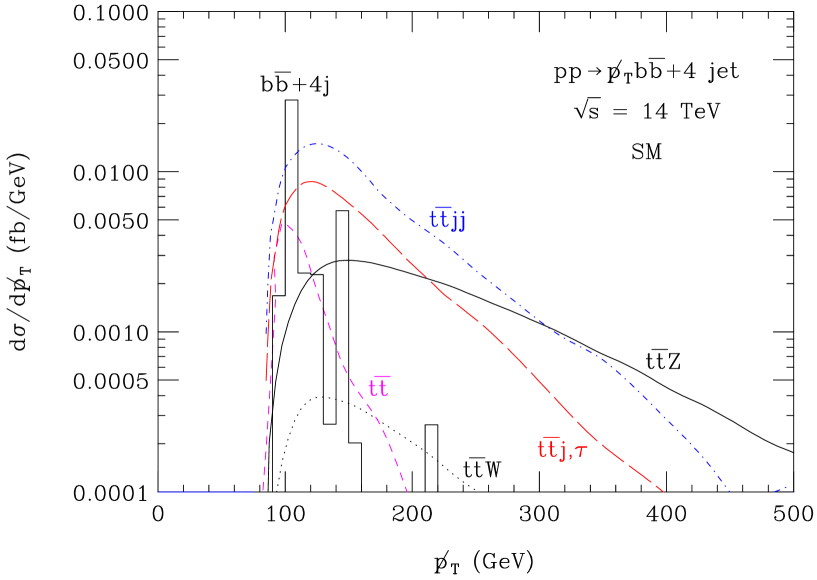
Figure 1: The differential cross sections as a function of missing transverse momentum for $p\hbox to0.0pt{\hss/}_{T}b\bar{b}+4j$ production at the LHC. Shown are the SM predictions for $t\bar{t}Z$ production and various backgrounds. We impose the cuts of Eqs. (II.2–10), but do not include the double $b$-tag efficiency common to all curves.

In Fig. 1 we show the missing transverse momentum distributions for the SM $t\bar{t}Z$ signal (solid curve) and for various backgrounds. The $p\hbox to0.0pt{\hss/}_{T}$ requirement of Eq. (5) implies that $p\hbox to0.0pt{\hss/}_{T}>80$ GeV. The most important backgrounds originate from $t\bar{t}jj$ and $t\bar{t}j$ production. However, the missing transverse momentum distribution from these processes falls considerably faster than that of the signal: for $p\hbox to0.0pt{\hss/}_{T}>300$ GeV, the SM signal dominates. The $t\bar{t}W$ background (dotted line) is about one order of magnitude smaller than the signal. The $t\bar{t}$ (dashed line) and $b\bar{b}$+$4j$ (histogram) backgrounds are important only at low values of $p\hbox to0.0pt{\hss/}_{T}$. Since the missing transverse momentum in these events originates entirely from $b$-decays and mismeasurements, their $p\hbox to0.0pt{\hss/}_{T}$ distributions fall very rapidly. This is even more the case for the $6j$ background which we found to essentially vanish after cuts. The $t\bar{t}jj$, $t\bar{t}\to\tau^{+}\nu_{\tau}\tau^{-}\bar{\nu}_{\tau}b\bar{b}\to p\hbox to0.0pt{\hss/}_{T}b\bar{b}jj$ background is found to be about four orders of magnitude smaller than the signal, thus is not shown.

The background contributions of $Zb\bar{b}$+$4j$, calculated with alpgen Mangano:2002ea , and $WZb\bar{b}jj$, $t\bar{b}Zjj$ and $\bar{t}bZjj$ production, calculated with madevent Maltoni:2002qb , are not shown in Fig. 1. As discussed in Ref. Baur:2004uw , these cross sections are one to two orders of magnitude smaller than the signal and can safely be neglected here.

It should be noted that the background cross sections as calculated at tree level depend significantly on the choice of factorization and renormalization scales, $\mu_{F}$ and $\mu_{R}$, which were taken to be $\mu_{F}=\mu_{R}=m_{t}$ in all cases, even for backgrounds without resonant top quarks. Including next-to-leading order (NLO) corrections in most cases significantly reduces the scale dependence of a process. Unfortunately, the NLO QCD corrections are not presently known for any of the background processes, except for $t\bar{t}$ production Beneke:2000hk ; lhctop . However, as we shall discuss in Sec. III.1, it may be possible to extract the background cross sections using data. For the dominant $t\bar{t}j(j)j$ backgrounds this should provide a more accurate estimate of the cross section than the leading order QCD predictions.

The $p\hbox to0.0pt{\hss/}_{T}$ distribution for $pp\to t\bar{t}Z$ in the SM (after decays), and for various anomalous $ttZ$ couplings, together with the combined $p\hbox to0.0pt{\hss/}_{T}$ distribution of the $t\bar{t}$, $b\bar{b}+4j$, $t\bar{t}j$ and $t\bar{t}jj$ backgrounds, are shown in Fig. 2.

Figure 2: The differential cross sections as a function of missing transverse momentum for $p\hbox to0.0pt{\hss/}_{T}b\bar{b}$+$4j$ production at the LHC. Shown are the SM predictions for $t\bar{t}Z$ production (solid line), the combined $t\bar{t}$, $b\bar{b}+4j$, $t\bar{t}j$ and $t\bar{t}jj$ background, and the predictions for several non-standard $ttZ$ couplings. Only one coupling at a time is allowed to deviate from its SM value. We impose the cuts of Eqs. (II.2–10), but do not include the double $b$-tag efficiency common to all curves.

Only one coupling at a time is allowed to deviate from its SM prediction. Fig. 2 shows that, as in the case when the $Z$ boson decays leptonically Baur:2004uw , varying $F^{Z}_{1V,A}$ leads mostly to a normalization change of the SM signal cross section, hardly affecting the shape of the $p\hbox to0.0pt{\hss/}_{T}$ distribution. Thus, the low-$p\hbox to0.0pt{\hss/}_{T}$ region contributes most of the statistical weight when extracting bounds on $F^{Z}_{1V,A}$. Since the signal $p\hbox to0.0pt{\hss/}_{T}$ distribution is approximately proportional to $(F^{Z}_{1V})^{2}+(F^{Z}_{1A})^{2}$, it is difficult to disentangle vector and axial vector couplings in the $p\hbox to0.0pt{\hss/}_{T}b\bar{b}$+$4j$ final state. Furthermore, $F^{Z}_{1V,A}=F^{Z,SM}_{1V,A}$ and $F^{Z}_{1V,A}=-F^{Z,SM}_{1V,A}$ yield approximately the same cross sections.

The dimension five couplings, $F^{Z}_{2V,A}$, on the other hand, lead to a missing transverse momentum distribution significantly harder than that predicted by the SM. As a result, most of the sensitivity to $F^{Z}_{2V,A}$ originates from the high-$p\hbox to0.0pt{\hss/}_{T}$ region. While the background is about one order of magnitude larger than the signal close to $p\hbox to0.0pt{\hss/}_{T}$ threshold, it is smaller than the signal for $p\hbox to0.0pt{\hss/}_{T}>380$ GeV. As a result, the limits extracted for $F^{Z}_{2V,A}$ depend considerably less on the background than those for $F^{Z}_{1V,A}$.

As stated before, we require that both $b$ quarks be tagged. A looser requirement of at least one tagged $b$ quark would result in a signal cross section increase of a factor $(2/\epsilon_{b}-1)$, about 2.2 using our $b$-tagging assumption. But this larger signal rate comes at the expense of an increased background. In particular, the $6j$ and $b\bar{b}$+$4j$ backgrounds increase drastically due to the larger combinatorial background from grouping jets and the tagged $b$ quark. Detailed calculations would be needed for a quantitative estimate of the increase. However, since the single-$b$-tagged background is probably considerably larger than that for the double $b$-tagged channel, we do not consider it here.

III Anomalous Couplings Limits and Model Implications

III.1 Limits on anomalous $\boldsymbol{ttZ}$ couplings

The shape and normalization changes of the $p\hbox to0.0pt{\hss/}_{T}$ spectrum can be used to derive quantitative sensitivity bounds on anomalous $ttZ$ couplings. We do this by performing a log-likelihood test on the distribution and calculating $68\%$ confidence level (CL) limits. To calculate the statistical significance, we split the $p\hbox to0.0pt{\hss/}_{T}$ distribution into bins, each with typically more than five events. We impose the cuts described in Sec. II.2 and assume a double $b$-tag efficiency of $\epsilon_{b}^{2}=0.4$. Except for the $ttZ$ couplings we assume the SM to be valid: the $tbW$ and $ttg$ couplings can be independently and precisely measured at the LHC in single top Boos:1999dd and $t\bar{t}$ production Beneke:2000hk , respectively. We perform multi-parameter fits for the different anomalous couplings, which we assume to be real.

The log-likelihood function we use to compute confidence levels is

$$-2\log L = -2\left[\sum_{i}\left(-f_{S}S_{i}-f_{B}B_{i}+n_{0i}\log(f_{S}S_{i}+f_{B}B_{i})-\log(n_{0i}!)\right)\right]$$ (11)

$$+\frac{(f_{S}-1)^{2}}{(\Delta f_{S})^{2}}+\frac{(f_{B}-1)^{2}}{(\Delta f_{B})^{2}}\,,$$

where the sum extends over the number of bins, $S_{i}$ and $B_{i}$ are the number of signal and background events in the $i$th bin, and $n_{0i}$ is the number of SM events in the $i$th bin. The uncertainties on the signal and background normalizations are taken into account via two multiplicative factors, $f_{S}$ and $f_{B}$, which are allowed to vary but are constrained within the relative uncertainties of the signal and background cross sections, $\Delta f_{S}$ and $\Delta f_{B}$, respectively.

To derive sensitivity bounds, we take into account the dominant $t\bar{t}jj$, $t\bar{t}j$, $t\bar{t}$ and $b\bar{b}$+$4j$ backgrounds. We calculate limits for 300 fb^-1 and 3000 fb^-1. An integrated luminosity of 300 fb^-1 corresponds to 3 years of running at the LHC design luminosity of ${\cal L}=10^{34}\,{\rm cm}^{-2}\,s^{-1}$, while the larger value of 3000 fb^-1 can be achieved in about 3 years of running at the luminosity-upgraded LHC (SLHC) Gianotti:2002xx .

As mentioned in Sec. II, the dimension five couplings $F^{Z}_{2V,A}$ lead to a considerably harder $p\hbox to0.0pt{\hss/}_{T}$ distribution than that predicted by the SM. Most of the sensitivity to these couplings thus originates from the high missing transverse momentum region. In this region, the signal to background ratio is of ${\cal O}(1)$ or better (cf. Fig. 2). The sensitivity bounds on $F^{Z}_{2V,A}$ should therefore depend very little on the normalization uncertainties of signal and background.

For $F^{Z}_{1V,A}$, however, the situation is different. Since the vector and axial vector couplings essentially change only the overall normalization of the $t\bar{t}Z$ cross section, precise knowledge of the SM signal cross section is very important. Most of the sensitivity to $F^{Z}_{1V,A}$ comes from the region of small $p\hbox to0.0pt{\hss/}_{T}$ where the background dominates over the signal. The achievable bounds on these couplings are thus expected to depend sensitively on the signal and background cross section uncertainties.

As explained before, except for the $t\bar{t}$ background, QCD corrections for neither the signal nor the background cross sections are known. The cross sections of the main backgrounds, $t\bar{t}jj$ and $b\bar{b}$+$4j$ production, are proportional to $\alpha_{s}^{4}$ and $\alpha_{s}^{6}$, respectively, whereas the signal cross section scales as $\alpha_{s}^{2}$. The background thus depends more strongly on the factorization and renormalization scales than the signal. Its normalization can be fixed by relaxing the selection cuts (Eqs. (6) and (10)), measuring the cross section in a background-dominated region of phase space, and then extrapolating to the analysis region. Since the cross sections for $t\bar{t}jj$ and $b\bar{b}$+$4j$ production are large, this should make it possible to determine the background with an uncertainty ($\Delta f_{B}$) of a few percent, provided that the systematic uncertainties can be adequately controlled and that the QCD corrections do not significantly change the shape of the $p\hbox to0.0pt{\hss/}_{T}$ distribution of the background. Exactly how well this will work in practice remains an open question.

To reduce the signal cross section uncertainty, the NLO QCD corrections to $t\bar{t}Z$ production must be calculated. This appears to be feasible with current techniques. Once the corrections are known, the remaining uncertainty ($\Delta f_{S}$) is likely to be of order $10\%$.

To derive quantitative sensitivity limits for anomalous $ttZ$ couplings, we assume $\Delta f_{S}=0.1$ and $\Delta f_{B}=0.05$. Unfortunately, the minimization of $-2\log L$ with respect to $f_{S}$ and $f_{B}$ cannot be performed analytically. Doing it numerically becomes very time consuming when more than one of the $ttZ$ couplings are varied at the same time. However, if one does not allow the signal and background normalizations to vary independently, i.e. if $f_{S}=f_{B}=f$, $\log L$ can be minimized analytically. In this case, one finds the minimum of $\log L$ to occur at

$$f=\frac{1}{2}\left(1-(\Delta f)^{2}N+\sqrt{(1-(\Delta f)^{2}N)^{2}+4(\Delta f)^{2}N_{0}}\right)\,,$$ (12)

where

$$N=\sum_{i}(S_{i}+B_{i})$$ (13)

is the total number of events,

$$N_{0}=\sum_{i}n_{0i}$$ (14)

the total number of SM events, and $\Delta f$ is the SM cross section uncertainty. The computer time required to derive sensitivity limits for anomalous $ttZ$ couplings is now much reduced.

The $68\%$ CL bounds on $\Delta F^{Z}_{1V,A}$ we obtain for $\Delta f_{S}=0.1$ and $\Delta f_{B}=0.05$ agree with those derived for $f_{S}=f_{B}=f$ and $\Delta f=0.3$ within $10-30\%$. In view of the current signal and background cross section uncertainties, an analysis with $f_{S}=f_{B}=f$ and $\Delta f=0.3$ when all couplings are varied should be sufficient. At first, it may be somewhat surprising that one needs $\Delta f$ to be significantly larger than $\Delta f_{S}$ and $\Delta f_{B}$ in order to arrive at similar bounds for non-standard $ttZ$ couplings. However, varying the signal and background cross section normalizations separately allows for changes in both the normalization and the shape of the SM cross section. On the other hand, requiring $f_{S}=f_{B}=f$ allows for only a change in the normalization. Since the anomalous $ttZ$ coupling sensitivity results from both normalization and $p\hbox to0.0pt{\hss/}_{T}$ distribution shape changes, taking into account the uncertainty on both naturally has a relatively larger impact than if only the normalization uncertainty is included in the analysis. One can partially compensate for this effect by increasing $\Delta f$.

Figure 3: Projected $68.3\%$ CL bounds on anomalous $ttZ$ couplings from the LHC with an integrated luminosity of 300 fb^-1, for: (a) $\Delta F^{Z}_{1A}$ versus $\Delta F^{Z}_{1V}$, (b) $\Delta F^{Z}_{2V}$ versus $\Delta F^{Z}_{1A}$, (c) $\Delta F^{Z}_{2V}$ versus $\Delta F^{Z}_{1V}$, and (d) $\Delta F^{Z}_{2A}$ versus $\Delta F^{Z}_{2V}$. Shown are the limits obtained from the $p\hbox to0.0pt{\hss/}_{T}b\bar{b}$+$4j$ (dashed) and the dilepton and trilepton final states (dotted), and the combined limits (solid). To derive limits for the dilepton and trilepton final states, we use the results of Ref. Baur:2004uw . In each graph, only those couplings which are plotted against each other are assumed to be different from their SM values.

Figure 4: Projected $68.3\%$ CL bounds on anomalous $ttZ$ couplings from the SLHC with an integrated luminosity of 3000 fb^-1, for: (a) $\Delta F^{Z}_{1A}$ versus $\Delta F^{Z}_{1V}$, (b) $\Delta F^{Z}_{2V}$ versus $\Delta F^{Z}_{1A}$, (c) $\Delta F^{Z}_{2V}$ versus $\Delta F^{Z}_{1V}$, and (d) $\Delta F^{Z}_{2A}$ versus $\Delta F^{Z}_{2V}$. Shown are the limits obtained from the $p\hbox to0.0pt{\hss/}_{T}b\bar{b}$+$4j$ (dashed) and the dilepton and trilepton final states (dotted), and the combined limits (solid). To derive limits for the dilepton and trilepton final states, we use the results of Ref. Baur:2004uw . In each graph, only those couplings which are plotted against each other are assumed to be different from their SM values.

Our results are shown in Figs. 3 and 4, and in Table 1. Fig. 3 shows the correlations between various anomalous $ttZ$ couplings for an integrated luminosity of 300 fb^-1; Fig. 4 displays the bounds one can hope to achieve at the SLHC with 3000 fb^-1. Shown are the results for the $p\hbox to0.0pt{\hss/}_{T}b\bar{b}$+$4j$ final state (dashed lines), the combined limits from the dilepton and trilepton final states analyzed in Ref. Baur:2004uw (dotted lines), and the limits resulting from combining all final states (solid lines). Including the $p\hbox to0.0pt{\hss/}_{T}b\bar{b}$+$4j$ final state in the extraction of bounds improves the limits by $10-60\%$. For an integrated luminosity of 300 fb^-1, it will be possible to measure the $ttZ$ axial vector coupling with a precision of about $10\%$, and $F^{Z}_{2V,A}$ with a precision of $40\%$. At the SLHC, these bounds can be improved by factors of about 1.6 ($F^{Z}_{2V,A}$) and $2.3-3$ ($F^{Z}_{1A}$). The achievable bounds on $F^{Z}_{1V}$ are much weaker than those projected for $F^{Z}_{1A}$: as mentioned in Sec. III, the $p\hbox to0.0pt{\hss/}_{T}$ distributions for the SM and for $F^{Z}_{1V,A}=-F^{Z,SM}_{1V,A}$ are almost degenerate. As a result, an area centered at $\Delta F^{Z}_{1V,A}=-2F^{Z,SM}_{1V,A}$ remains, which cannot be excluded, even at the SLHC where one expects several thousand $t\bar{t}Z$ events. For $F^{Z}_{1V}$, the two regions merge, resulting in rather poor limits. For $F^{Z}_{1A}$, the two regions are distinct. Since the area centered at $\Delta F^{Z}_{1A}=-2F^{Z,SM}_{1A}$ is incompatible with the indirect limits on the $ttZ$ vector and axial vector couplings from $Z$-pole data Baur:2004uw , we do not include this are in Table 1 or Figs. 3 and 4.

While the bounds on $\Delta F^{Z}_{1A}$ improve by $20-60\%$ when the $p\hbox to0.0pt{\hss/}_{T}b\bar{b}$+$4j$ channel is included in the analysis, the gain is limited to about $10\%$ for $\Delta F^{Z}_{1V}$. The global limits on the dimension-five couplings $F^{Z}_{2V,A}$ improve by about $20\%$. However, if only $F^{Z}_{2V}$ and $F^{Z}_{2A}$ are varied, including the $p\hbox to0.0pt{\hss/}_{T}b\bar{b}$+$4j$ final state strengthens their bounds by about $35\%$. The relatively larger importance of the $p\hbox to0.0pt{\hss/}_{T}b\bar{b}$+$4j$ channel in this case can be understood by recalling that most of the sensitivity to the dimension-five couplings originates from high $p\hbox to0.0pt{\hss/}_{T}$ values where the background is less important. This allows one to take better advantage of the larger $p\hbox to0.0pt{\hss/}_{T}b\bar{b}$+$4j$ final state cross section.

The correlations between $F^{Z}_{2A}$ and $F^{Z}_{1A}$ ($F^{Z}_{2A}$ and $F^{Z}_{1V}$) are similar to those for $F^{Z}_{2V}$ and $F^{Z}_{1A}$ ($F^{Z}_{2V}$ and $F^{Z}_{1V}$), thus are not shown in Figs. 3 and 4.

300 fb-1 (LHC)				3000 fb-1 (SLHC)
coupling	$p\hbox to0.0pt{\hss/}_{T}b\bar{b}$+$4j$	$2\ell$+$3\ell$	combined	coupling	$p\hbox to0.0pt{\hss/}_{T}b\bar{b}$+$4j$	$2\ell$+$3\ell$	combined
$\Delta F^{Z}_{1V}$	–	$\begin{matrix}+0.84\\[-4.0pt] -0.43\end{matrix}$	$\begin{matrix}+0.75\\[-4.0pt] -0.36\end{matrix}$	$\Delta F^{Z}_{1V}$	–	$\begin{matrix}+0.60\\[-4.0pt] -0.18\end{matrix}$	$\begin{matrix}+0.54\\[-4.0pt] -0.16\end{matrix}$
$\Delta F^{Z}_{1A}$	$\begin{matrix}+0.12\\[-4.0pt] -\end{matrix}$	$\begin{matrix}+0.16\\[-4.0pt] -0.13\end{matrix}$	$\begin{matrix}+0.096\\[-4.0pt] -0.112\end{matrix}$	$\Delta F^{Z}_{1A}$	$\begin{matrix}+0.047\\[-4.0pt] -\end{matrix}$	$\begin{matrix}+0.049\\[-4.0pt] -0.060\end{matrix}$	$\begin{matrix}+0.031\\[-4.0pt] -0.048\end{matrix}$
$\Delta F^{Z}_{2V}$	$\begin{matrix}+0.59\\[-4.0pt] -0.55\end{matrix}$	$\begin{matrix}+0.47\\[-4.0pt] -0.47\end{matrix}$	$\begin{matrix}+0.38\\[-4.0pt] -0.39\end{matrix}$	$\Delta F^{Z}_{2V}$	$\begin{matrix}+0.34\\[-4.0pt] -0.32\end{matrix}$	$\begin{matrix}+0.28\\[-4.0pt] -0.28\end{matrix}$	$\begin{matrix}+0.25\\[-4.0pt] -0.24\end{matrix}$
$\Delta F^{Z}_{2A}$	$\begin{matrix}+0.57\\[-4.0pt] -0.58\end{matrix}$	$\begin{matrix}+0.48\\[-4.0pt] -0.49\end{matrix}$	$\begin{matrix}+0.40\\[-4.0pt] -0.40\end{matrix}$	$\Delta F^{Z}_{2A}$	$\begin{matrix}+0.33\\[-4.0pt] -0.33\end{matrix}$	$\begin{matrix}+0.28\\[-4.0pt] -0.29\end{matrix}$	$\begin{matrix}+0.25\\[-4.0pt] -0.25\end{matrix}$

Table 1: Sensitivities achievable at $68.3\%$ CL for anomalous $ttZ$ couplings at the LHC and SLHC for integrated luminosities of 300 fb^-1, and 3000 fb^-1. The limits shown represent the maximum and minimum values obtained when taking into account the correlations between any possible pair of anomalous couplings. Results are for the $p\hbox to0.0pt{\hss/}_{T}b\bar{b}$+$4j$ final state, the combined dilepton and trilepton final states analyzed in Ref. Baur:2004uw (labeled $2\ell+3\ell$), and for all channels combined. The cuts imposed are described in Sec. II.2.

The $ttZ$ couplings are indirectly constrained by precision $Z$-pole data collected at LEP and SLC. Vector and axial vector couplings are bound by $Z$-boson data to within a few percent of their SM values if one assumes that no other sources of new physics contribute. In contrast, the limits obtained for $F^{Z}_{2V}$ are much weaker, $|F^{Z}_{2V}|\lesssim{\cal O}(0.2)$, and depend on the value of the anomalous magnetic moment of the top quark Eboli:1997kd . The effect of $F^{Z}_{2A}$ on LEP/SLC observables has not yet been studied. Thus, $t\bar{t}Z$ production at the LHC will provide valuable information on the dimension-five couplings. Since the LEP/SLC constraints arise from one-loop corrections which diverge for non-standard $ttZ$ couplings, they are cutoff-dependent. When taking into account the $p\hbox to0.0pt{\hss/}_{T}b\bar{b}$+$4j$ final state, the achievable sensitivity on $F^{Z}_{1A}$ at the SLHC begins to approach that of the indirect bounds from $Z$-pole data. For the $ttZ$ vector coupling, it will be impossible to match that precision at the LHC, even for an integrated luminosity of 3000 fb^-1 and including the $p\hbox to0.0pt{\hss/}_{T}b\bar{b}$+$4j$ final state in the analysis.

The $ttZ$ couplings can also be tested in $e^{+}e^{-}\to t\bar{t}$. However, as mentioned in Sec. I, the process $e^{+}e^{-}\to\gamma^{*},\,Z^{*}\to t\bar{t}$ is sensitive to both $tt\gamma$ and $ttZ$ couplings simultaneously. If only one coupling at a time is allowed to deviate from its SM value, a linear $e^{+}e^{-}$ collider operating at $\sqrt{s}=500$ GeV with an integrated luminosity of $100-200$ fb^-1 would be able to probe all $ttZ$ couplings with a precision of $1-5\%$ Abe:2001nq . With the possible exception of $F^{Z}_{1A}$, a linear collider will thus be able to significantly improve the sensitivity limits expected from the LHC, even when the $p\hbox to0.0pt{\hss/}_{T}b\bar{b}$+$4j$ channel is included and assuming 3000 fb^-1 from the SLHC. It should be noted, however, that this picture could change once cancellations between different non-standard $ttZ$ couplings, and between $tt\gamma$ and $ttZ$ couplings, are allowed. While beam polarization at an $e^{+}e^{-}$ collider would provide a very powerful tool to disentangle the effects of different couplings, unfortunately no realistic studies on the simultaneous measurement of couplings in $e^{+}e^{-}\to t\bar{t}$ have been performed so far.

III.2 Constraints on Little Higgs parameter space

As noted in Sec. I, the $ttZ$ couplings may deviate substantially from their SM values in Little Higgs (LH) models. Here we explore how their measurement at the LHC may constrain parameter space in the $SU(5)/SO(5)$ Littlest Higgs model with T-parity Cheng:2003ju ; Cheng:2004yc ; Low:2004xc . In this model, the $ttZ$ vector and axial vector couplings are modified by mixing of the left-handed top quark and a heavy top quark partner, $T$. One finds

$$\Delta F^{Z}_{1V}=-\Delta F^{Z}_{1A}=\frac{\lambda_{T}^{2}v^{2}}{2m_{T}^{2}}\,F^{Z,SM}_{1A}\,,$$ (15)

where $\lambda_{T}$ is the $tTh$ coupling ($h$ is the Higgs boson), $v\approx 246$ GeV is the SM Higgs vacuum expectation value, and $m_{T}$ is the $T$ quark mass. Eq. (15) and the log likelihood function can be used to derive lower $68.3\%$ CL limits for $m_{T}/\lambda_{T}$:

$$\frac{m_{T}}{\lambda_{T}} \geq 600~{}{\rm GeV}\qquad{\rm for~{}300~{}fb^{-1},}$$ (16)

$$\frac{m_{T}}{\lambda_{T}} \geq 1000~{}{\rm GeV}\qquad{\rm for~{}3000~{}fb^{-1}.}$$ (17)

For comparison, current EW precision data require $m_{T}/\lambda_{T}>650$ GeV Hubisz:2005tx . We thus expect the SLHC will be able to improve this bound, while the LHC should be able to discover a $T$ quark with a mass of $m_{T}\leq 2$ TeV with 300 fb^-1 of data Azuelos:2004dm . If a $T$-quark candidate were found, a measurement of $F^{Z}_{1A}$ would be valuable in helping to pin down $\lambda_{T}$.

In LH models without T-parity, anomalous $ttZ$ couplings may receive additional contributions from mixing of the $W$ and $Z$ bosons with a heavy $SU(2)$ triplet of vector bosons, $W^{\pm}_{H}$ and $W^{3}_{H}$, which are characteristic for LH models Berger:2005ht . However, constraints from precision EW data severely restrict these additional contributions.

IV Summary and Conclusions

Currently, little is known about top quark couplings to the $Z$ boson. There are no direct measurements of these couplings; indirect measurements, using LEP and SLC data, tightly constrain only the $ttZ$ vector and axial vector couplings. The $ttZ$ couplings could be measured directly in $e^{+}e^{-}\to t\bar{t}$ at a future $e^{+}e^{-}$ linear collider. However, such a machine is at least a decade away. In addition, the process $e^{+}e^{-}\to t\bar{t}$ is simultaneously sensitive to $tt\gamma$ and $ttZ$ couplings, and significant cancellations between various couplings may occur.

In this paper, we considered $t\bar{t}Z$ production with $Z\to\bar{\nu}\nu$ and $t\bar{t}\to b\bar{b}$+$4j$ at the LHC as a tool to measure $ttZ$ couplings. At the Tevatron, the $t\bar{t}Z$ cross section is too small to be observable. When the $Z$ boson decays leptonically, the small $Z\to\ell^{+}\ell^{-}$ branching ratio is one of the main factors which limits the achievable sensitivity to anomalous $ttZ$ couplings. The larger $Z\to\bar{\nu}\nu$ branching ratio (relative to $Z\to\ell^{+}\ell^{-}$) effectively triples the number of signal events and thus has the potential to significantly improve the sensitivity to non-standard couplings.

We calculated the signal cross sections taking into account all top quark-resonant Feynman diagrams. All relevant background processes were included in estimating limits on the couplings. Once $t\bar{t}Z$ selection cuts are imposed, the background drops significantly faster with missing transverse momentum than the signal, and for $p\hbox to0.0pt{\hss/}_{T}>380$ GeV the signal dominates. The largest background source is $t\bar{t}jj$ production, where one of the top quarks decays semi-leptonically and the charged lepton is lost. In all our calculations we assumed that both $b$ quarks are tagged, to bring the backgrounds to a controllable level.

Our analysis reveals that the achievable sensitivity limits utilizing final states where the $Z$ decays leptonically Baur:2004uw can be improved by $10-60\%$ when the $p\hbox to0.0pt{\hss/}_{T}b\bar{b}$+$4j$ mode is taken into account. The improvement is particularly pronounced for the $ttZ$ axial vector coupling $F^{Z}_{1A}$ which can be measured with a precision of $3-5\%$ at the luminosity-upgraded LHC (3000 fb^-1). Measuring $F^{Z}_{1A}$ with such precision will make it possible constrain the parameter space in Little Higgs models which predict deviations of the $ttZ$ vector and axial vector couplings of up to $10\%$.