Production and decays of supersymmetric Higgs bosons in spontaneously broken R-parity

Abstract

We study the mass spectra, production and decay properties of the lightest supersymmetric CP-even and CP-odd Higgs bosons in models with spontaneously broken R-parity (SBRP). We compare the resulting mass spectra with expectations of the Minimal Supersymmetric Standard Model (MSSM), stressing that the model obeys the upper bound on the lightest CP-even Higgs boson mass. We discuss how the presence of the additional scalar singlet states affects the Higgs production cross sections, both for the Bjorken process and the “associated production”. The main phenomenological novelty with respect to the MSSM comes from the fact that the spontaneous breaking of lepton number leads to the existence of the majoron, denoted $J$, which opens new decay channels for supersymmetric Higgs bosons. We find that the invisible decays of CP-even Higgses can be dominant, while those of the CP-odd bosons may also be sizeable.

I Introduction

Unveiling the mechanism of symmetry breaking and mass generation constitutes one of the main goals in the agenda of upcoming accelerators, like CERN’s Large Hadron Collider (LHC) and the International Linear Collider (ILC). Precision electroweak data currently hint that the mechanism responsible for electroweak symmetry breaking Carena:2002es involves a weakly-coupled Higgs sector, as predicted by supersymmetry. Supersymmetry also stabilizes the Higgs boson mass against quadratic divergences, thus accounting for the hierarchy between the electroweak and the Planck scales in a technically natural way. A very exciting possibility is that the experimentally observed McDonald:2004dd ; Kajita:2004ga ; Araki:2004mb neutrino masses and mixings Maltoni:2004ei have a supersymmetric origin Hirsch:2004he . The key requirement for this to be possible is that R–parity, defined as $R_{p}=(-1)^{3B+L+2S}$ (with $S$, $B$, $L$ denoting spin, baryon and lepton numbers, respectively) be violated. The simplest way to do this is through a bilinear term in the superpotential.

The resulting model is interesting in two ways. First it provides the most economical description of R-parity violation as a “perturbation” to the Minimal Supersymmetric Standard Model: it may be taken as the reference R-parity violation model, which we may call RMSSM diaz:1998xc . The model offers a minimal low-scale mechanism to generate neutrino masses, that successfully accounts for the observed pattern of neutrino masses and mixing Hirsch:2000ef ; romao:1999up  . In contrast to the seesaw mechanism, it makes well defined predictions that will be tested at upcoming colliders LHC/ILC, namely, the decay branching ratios of the lightest supersymmetric particle are related to the neutrino mixing angles measured in neutrino experiments porod:2000pw .

On the other hand the model also provides the simplest effective description of theories where the breaking of R-parity occurs spontaneously, like that of the electroweak gauge symmetry itself, due to the existence of non-zero singlet sneutrino vacuum expectation values (vevs) masiero:1990uj ; romao:1992vu ; romao:1997xf ; shiraishi:1993di . A general feature of models where neutrino masses arise from low-scale spontaneous violation of ungauged lepton number is that the lightest CP-even supersymmetric Higgs boson will have an important decay channel into the singlet Goldstone boson (called majoron) associated to lepton number violation Joshipura:1993hp :

$$h\to JJ\,.$$ (1)

Thus the Higgs boson may decay mainly to an invisible mode characterized by missing energy, instead of the Standard Model channels. This general possibility can also be realized in spontaneously broken R–parity supersymmety romao:1992zx .

We have recently reanalyzed this suggestion in view of the data on neutrino oscillations that indicate non-zero neutrino masses Hirsch:2004rw . We found that this proposal remains valid, despite the smallness of neutrino masses required to fit current neutrino oscillation data Maltoni:2004ei . In Ref. Hirsch:2004rw we have shown explicitly that the invisible decays of the lightest CP-even Higgs boson can be dominant, unsuppressed by the small neutrino masses, for the same parameter values for which Higgs production in $e^{+}e^{-}$ annihilation is comparable in cross section to that characterizing the standard case. A necessary ingredient in this case is the existence of an SU(2) $\otimes$ U(1) singlet superfield $\Phi$ coupling to the electroweak doublet Higgses, which may provide a solution to the so-called $\mu$-problem.

In this follow-up paper we extend the analysis and study in detail the possibility that the lightest CP-even Higgs boson is produced also in association with a CP-odd boson in electron-positron collisions. The first aspect to consider is the theoretically expected mass spectra of CP-even and CP-odd scalar bosons. An important feature of any supersymmetric model is the existence of an upper bound on the mass of the lightest CP-even scalar boson. We verify explicitly that this feature emerges in the present model. We also explain how the supersymmetric Higgs boson mass upper limit should be understood in terms of the SBRP model fields.

Then we turn to the Higgs production cross sections. Although individual Higgs boson production cross sections, via the familiar Bjorken process or the associated mode, are potentially suppressed with respect to those of the MSSM, given enough center-of-mass energy and luminosity, all Higgses can be potentially explored due to unitarity. We carefully analyze the decay properties of the first and second lightest Higgs bosons. The case of the lightest CP-even Higgs boson was already considered in Ref. Hirsch:2004rw . We revisit this case, and confirm that the invisible dacay mode for either the first or the second lightest CP-even Higgs boson can easily dominate, in contrast to that of the lightest CP-odd which may arise at subleading level up to 20 % level at most.

II The Model

For completeness we recall here the main ingredients of the model. In addition to the Minimal Supersymmetric Standard Model superfields it contains SU(2) $\otimes$ U(1) singlet superfields $({\widehat{\nu}^{c}}_{i},\widehat{S}_{i},{\widehat{\Phi}})$ carrying lepton number assigned as $(-1,1,0)$. With this choice the most general superpotential terms conserving lepton number are given as romao:1992zx

$${\cal W} \hskip-11.38109pt=\hskip-11.38109pt \varepsilon_{ab}\Big{(}h_{U}^{ij}\widehat{Q}_{i}^{a}\widehat{U}_{j}\widehat{H}_{u}^{b}+h_{D}^{ij}\widehat{Q}_{i}^{b}\widehat{D}_{j}\widehat{H}_{d}^{a}+h_{E}^{ij}\widehat{L}_{i}^{b}\widehat{E}_{j}\widehat{H}_{d}^{a}+h_{\nu}^{ij}\widehat{L}_{i}^{a}\widehat{\nu}^{c}_{j}\widehat{H}_{u}^{b}\!-{\hat{\mu}}\widehat{H}_{d}^{a}\widehat{H}_{u}^{b}\!-(h_{0}\widehat{H}_{d}^{a}\widehat{H}_{u}^{b}+\delta^{2})\widehat{\Phi}\Big{)}$$ (2)

$$+\hskip 14.22636pth^{ij}\widehat{\Phi}\widehat{\nu}^{c}_{i}\widehat{S}_{j}+M_{R}^{ij}\widehat{\nu}^{c}_{i}\widehat{S}_{j}+\frac{1}{2}M_{\Phi}\widehat{\Phi}^{2}+\frac{\lambda}{3!}\widehat{\Phi}^{3}\,.$$

The first three terms together with the ${\hat{\mu}}$ term define the R-parity conserving MSSM, the terms in the last row involve only couplings among the SU(2) $\otimes$ U(1) singlet superfields $({\widehat{\nu}^{c}}_{i},\widehat{S}_{i},{\widehat{\Phi}})$. The remaining terms couple the singlets to the MSSM fields. We stress the importance of the Dirac-Yukawa term which connects the right-handed neutrino superfields to the lepton doublet superfields, thus fixing lepton number.

Like all other Yukawa couplings in general $h_{\nu}$ is an arbitrary non-symmetric complex matrix in generation space. However, for technical simplicity we will consider only the case with just one pair of lepton–number–carrying SU(2) $\otimes$ U(1) singlet superfields, $\widehat{\nu}^{c}$ and $\widehat{S}$, in order to avoid inessential complication. This in turn implies, $h^{ij}\to h$ and $h_{\nu}^{ij}\to h_{\nu}^{i}$.

The scalar potential along neutral directions is given by

$$V_{total} = |h\Phi\tilde{S}+h_{\nu}^{i}\tilde{\nu}_{i}H_{u}+M_{R}\tilde{S}|^{2}+|h_{0}\Phi H_{u}+\hat{\mu}H_{u}|^{2}+|h\Phi\tilde{\nu^{c}}+M_{R}\tilde{\nu^{c}}|^{2}$$

$$+|-h_{0}\Phi H_{d}-\hat{\mu}H_{d}+h_{\nu}^{i}\tilde{\nu}_{i}\tilde{\nu^{c}}|^{2}+|-h_{0}H_{u}H_{d}+h\tilde{\nu^{c}}\tilde{S}-\delta^{2}+M_{\Phi}\Phi+\frac{\lambda}{2}\Phi^{2}|^{2}$$

$$+\sum_{i=1}^{3}|h_{\nu}^{i}\tilde{\nu^{c}}H_{u}|^{2}+\Big{[}A_{h}h\Phi\tilde{\nu^{c}}\tilde{S}-A_{h_{0}}h_{0}\Phi H_{u}H_{d}+A_{h_{\nu}}h_{\nu}^{i}\tilde{\nu}_{i}H_{u}\tilde{\nu^{c}}-B\hat{\mu}H_{u}H_{d}$$

$$-C_{\delta}\delta^{2}\Phi+B_{M_{R}}M_{R}\tilde{\nu^{c}}\tilde{S}+\frac{1}{2}B_{M_{\Phi}}M_{\Phi}\Phi^{2}+\frac{1}{3!}A_{\lambda}\lambda\Phi^{3}+h.c.\Big{]}$$

$$+\sum_{\alpha}\tilde{m}_{\alpha}^{2}|z_{\alpha}|^{2}+\frac{1}{8}(g^{2}+{g^{\prime}}^{2})\Big{(}|H_{u}|^{2}-|H_{d}|^{2}-\sum_{i=1}^{3}|\tilde{\nu}_{i}|^{2}\Big{)}^{2}\,,$$

where $z_{\alpha}$ denotes any neutral scalar field in the theory. For simplicity we assume CP conservation in the scalar sector, taking all couplings real.

Electroweak symmetry breaking is driven by the isodoublet vevs $\left\langle{H_{u}}\right\rangle=\frac{v_{u}}{\sqrt{2}}$ and $\left\langle{H_{d}}\right\rangle=\frac{v_{d}}{\sqrt{2}}$, with the combination $v^{2}=v_{u}^{2}+v_{d}^{2}+\sum_{i}v_{Li}^{2}$ fixed by the $W$ mass, while the ratio of isodoublet vevs yields $\tan\beta=\frac{v_{u}}{v_{d}}$. Here, $\frac{v_{Li}}{\sqrt{2}}$ are the vevs of the left-scalar neutrinos. They vanish in the limit where $h^{i}_{\nu}\to 0$. In this limit R–parity is restored and neutrinos become massless, as in the MSSM, and, apart from $\Phi$, the extra singlets become phenomenologically irrelevant, one reaches the NMSSM limit Panagiotakopoulos:2000wp ; Dedes:2000jp .

The spontaneous breaking of R-parity is driven by nonzero vevs for the right-scalar neutrinos. The scale characterizing R-parity breaking is set by the isosinglet vevs $\left\langle\tilde{\nu^{c}}\right\rangle=\frac{v_{R}}{\sqrt{2}}$ and $\langle\tilde{S}\rangle=\frac{v_{S}}{\sqrt{2}}$. Finally, $\left\langle\Phi\right\rangle=\frac{v_{\Phi}}{\sqrt{2}}$ gives a contribution to the $\mu$–term.

With the above choices and definitions we can obtain the neutral scalar boson mass matrices as described in Ref. romao:1992vu . This results in $8\times 8$ mass matrices for the real and imaginary parts of the neutral scalars. Their complete definition can be found in  Hirsch:2004rw . The spontaneous breaking of SU(2) $\otimes$ U(1) and lepton number leads to two Goldstone bosons, namely $G^{0}$ , the one “eaten” by the $Z^{0}$, as well as $J$, the majoron. In the basis $P^{\prime 0}=(H_{d}^{0I},H_{u}^{0I},\tilde{\nu}^{1I},\tilde{\nu}^{2I},\tilde{\nu}^{3I},\Phi^{I},\tilde{S}^{I},\tilde{\nu}^{cI})$ these fields are given as,

$$G^{0} = (N_{0}\,v_{d},-N_{0}\,v_{u},N_{0}\,v_{L1},N_{0}\,v_{L2},N_{0}\,v_{L3},0,0,0)\,$$

$$J = N_{4}(-N_{1}v_{d},N_{1}v_{u},N_{2}v_{L1},N_{2}v_{L2},N_{2}v_{L3},0,N_{3}v_{S},-N_{3}v_{R})\,,$$ (4)

where the normalization constants $N_{i}$ are given as

$$N_{0} = \frac{1}{\sqrt{v_{d}^{2}+v_{u}^{2}+v_{L1}^{2}+v_{L2}^{2}+v_{L3}^{2}}}$$

$$N_{1} = v_{L1}^{2}+v_{L2}^{2}+v_{L3}^{2}$$

$$N_{2} = v_{d}^{2}+v_{u}^{2}$$

$$N_{3} = N_{1}+N_{2}$$

$$N_{4} = \frac{1}{\sqrt{N_{1}^{2}N_{2}+N_{2}^{2}N_{1}+N_{3}^{2}(v_{R}^{2}+v_{S}^{2})}}$$ (5)

and can easily be checked to be orthogonal, i. e. they satisfy $G^{0}\cdot J=0$.

The neutrino masses and mixings arising from this model Hirsch:2004rw have been shown to reproduce the current data on neutrino oscillations that indicate non-zero neutrino masses Maltoni:2004ei . Since neutrino masses are so much smaller than all other fermion mass terms in the model, once can find the effective neutrino mass matrix in a seesaw–type approximation. After some algebraic manipulation, the effective neutrino mass matrix can be cast into a very simple form

$$(\boldsymbol{m_{\nu\nu}^{\rm eff}})_{ij}=a\Lambda_{i}\Lambda_{j}+b(\epsilon_{i}\Lambda_{j}+\epsilon_{j}\Lambda_{i})+c\epsilon_{i}\epsilon_{j}\,,$$ (6)

where one can define the effective bilinear R–parity violating parameters $\epsilon_{i}$ and $\Lambda_{i}$ as

$$\epsilon_{i}=h_{\nu}^{i}\,\frac{v_{R}}{\sqrt{2}}$$ (7)

and

$$\Lambda_{i}=\epsilon_{i}v_{d}+\mu v_{L_{i}}\,.$$ (8)

Here the parameter $\mu$ is

$$\mu=\hat{\mu}+h_{0}\frac{v_{\Phi}}{\sqrt{2}}\,,$$ (9)

while the coefficients appearing in Eq. (6) are given in Ref. Hirsch:2004rw . Eq. (6) resembles closely the structure found for the explicit bilinear model at the one-loop level. However, the coefficients are different, see Hirsch:2004rw .

Neutrino physics puts a number of constraints on the parameters $\Lambda_{i}$ and $\epsilon_{i}$. For the current paper, however, exact details are unimportant, the most essential constraint for the following discussion is that $h_{\nu}^{i}\ll 1$ is required. (See later discussion of left-sneutrino mixing. In the limit $h_{\nu}^{i}=0$ left-sneutrinos do not mix at all with Higgses and singlets).

The requirement that $v_{L_{i}}\ll v$ can be used to find a simple approximation formula for the majoron, given by

$$J\simeq(\frac{-v_{d}v_{L}^{2}}{Vv^{2}},\frac{v_{u}v_{L}^{2}}{Vv^{2}},\frac{v_{L1}}{V},\frac{v_{L2}}{V},\frac{v_{L3}}{V},0,\frac{v_{S}}{V},-\frac{v_{R}}{V})\,,$$ (10)

where $V^{2}=v_{S}^{2}+v_{R}^{2}$. Thus, the majoron is essentially made up of the ${\tilde{\nu}}^{c}$ and ${\tilde{S}}$ fields. This will be important later, when we discuss the decays of the Higgs bosons.

III Higgs spectrum

Let us first briefly discuss the spectrum of the scalar and pseudo-scalar sectors in the model. For detailed definitions we refer the reader to Ref. Hirsch:2004rw . Since these mass matrices are too complicated for analytic diagonalization, we will solve the exact eigensystems numerically. However, before doing that, we discuss certain limits, where some simplifying approximations are made. This allows us to gain some insight into the nature of the spectra.

In the SBRP model there are 8 neutral CP-even states $S^{0}_{i}$. In the neutral CP-odd sector there are six massive states $P^{0}_{i}$ ($i=1,\ldots,6$), in addition to the majoron $J$, with $m_{J}=0$, and the Goldstone $G^{0}$. We introduce the convention, to be discussed below:

$$\left(S^{0}\right)^{T} = \left(S_{h^{0}},S_{H^{0}},S_{J},S_{J_{\perp}},S_{\Phi},S_{\tilde{\nu}_{i}}\right)$$ (11)

$$\left(P^{0}\right)^{T} = \left(P_{A^{0}},P_{J_{\perp}},P_{\Phi},P_{\tilde{\nu}_{i}},J,G^{0}\right).$$

Note, that the ordering of these states is not by increasing mass, as we have defined $P^{0}_{i}$ ($i=1,\ldots,6$) as the massive states.

First we note that all entries in the sub-matrices which mix the left-sneutrinos to the doublet Higgses and the singlet states are proportional to $h^{i}_{\nu}$. In the region of parameters where the model accounts for the observed neutrino masses we must have that $\epsilon_{i}=h^{i}_{\nu}v_{R}/\sqrt{2}$ is necessarily a small number and therefore $h^{i}_{\nu}\ll 1$. Thus, left sneutrinos mix very little with the other (pseudo-)scalars, unless entries in the sneutrino sector are, by chance, highly degenerate with the ones in the other sectors. The real (imaginary) parts of these nearly-sneutrino states are denoted by $S_{\tilde{\nu}_{i}}$ ($P_{\tilde{\nu}_{i}}$) in the definition given above. Barring fine-tuned situations, we conclude that mixing between Higgses and left sneutrinos will, in general, be small.

Consider now the pseudoscalar sector,

$$\boldsymbol{M^{P^{2}}}=\left[\begin{array}[]{lll}\boldsymbol{M^{P^{2}}_{HH}}&\boldsymbol{M^{P^{2}}_{H\widetilde{L}}}&\boldsymbol{M^{P^{2}}_{HS}}\\[5.69054pt] \boldsymbol{M^{P^{2}}_{H\widetilde{L}}}\!{}^{\rm T}&\boldsymbol{M^{P^{2}}_{\widetilde{L}\widetilde{L}}}&\boldsymbol{M^{P^{2}}_{\widetilde{L}S}}\\[5.69054pt] \boldsymbol{M^{P^{2}}_{HS}}\!{}^{\rm T}&\boldsymbol{M^{P^{2}}_{\widetilde{L}S}}\!{}^{\rm T}&\boldsymbol{M^{P^{2}}_{SS}}\end{array}\right],$$ (15)

where $\boldsymbol{M^{P^{2}}_{HH}}$ is a symmetric $2\times 2$ matrix, $\boldsymbol{M^{P^{2}}_{\widetilde{L}\widetilde{L}}}$ and $\boldsymbol{M^{P^{2}}_{SS}}$ are symmetric $3\times 3$ matrices, while $\boldsymbol{M^{P^{2}}_{H\widetilde{L}}}$ and $\boldsymbol{M^{P^{2}}_{HS}}$ are $2\times 3$ matrices and finally $M^{P^{2}}_{\widetilde{L}S}$ is (a non-symmetric) $3\times 3$ matrix. In this notation $\widetilde{L}$ denotes the sneutrinos and $S$ the singlet fields.

Neglecting terms proportional to $h^{i}_{\nu}$, $\boldsymbol{M^{P^{2}}_{HH}}$ can be written as

$$\boldsymbol{M^{P^{2}}_{HH}}=\left[\begin{array}[]{ll}\Omega\frac{v_{u}}{v_{d}}&\Omega\\ \Omega&\Omega\frac{v_{d}}{v_{u}}\end{array}\right],$$ (18)

where 

$$\Omega=B\hat{\mu}-\delta^{2}h_{0}+\frac{\lambda}{4}h_{0}v_{\Phi}^{2}+\frac{1}{2}hh_{0}v_{R}v_{S}+\frac{\sqrt{2}}{2}A_{h_{0}}h_{0}v_{\Phi}+\frac{\sqrt{2}}{2}h_{0}M_{\Phi}v_{\Phi}\,.$$ (19)

Note the presence of $h_{0}$-dependent terms in Eq. (19). If there were no mixing between the doublet and singlet Higgses, Eq. (18) would yield the eigenvalues,

$$m^{2}_{1,2}=\Big{(}0,\Omega(\frac{v_{u}}{v_{d}}+\frac{v_{d}}{v_{u}})\Big{)}\,,$$ (20)

with the massless state identified as the Goldstone boson, $G^{0}$, and the other state as the pseudo-scalar Higgs $A^{0}$ of the MSSM, with

$$m^{2}_{A^{0}}=\frac{2\Omega}{\sin 2\beta}\,.$$ (21)

The state most closely resembling the MSSM $A^{0}$, i.e. the state remaining in the spectrum when singlets are decoupled is called $P_{A^{0}}$ in Eq. (11). The sub-matrix $\boldsymbol{M^{P^{2}}_{SS}}$, on the other hand, in the limit $h^{i}_{\nu}=0$, can be written as,

$$\boldsymbol{M^{P^{2}}_{SS}}=\left[\begin{array}[]{lll}M^{P^{2}}_{SS_{11}}&M^{P^{2}}_{SS_{12}}&M^{P^{2}}_{SS_{13}}\\ M^{P^{2}}_{SS_{12}}&-\Gamma\frac{v_{R}}{v_{S}}&-\Gamma\\ M^{P^{2}}_{SS_{13}}&-\Gamma&-\Gamma\frac{v_{S}}{v_{R}}\end{array}\right],$$ (25)

where,

$$M^{P^{2}}_{SS_{11}} = \delta^{2}\left(C_{\delta}+M_{\Phi}\right)\frac{\sqrt{2}}{v_{\Phi}}-\frac{\sqrt{2}}{2}(v_{d}^{2}+v_{u}^{2})\frac{h_{0}\hat{\mu}}{v_{\Phi}}-\frac{\sqrt{2}}{4}\lambda\left(3A_{\lambda}+M_{\Phi}\right)v_{\Phi}$$ (26)

$$- 2B_{M_{\Phi}}M_{\Phi}-\frac{\sqrt{2}}{2}h\left(A_{h}+M_{\Phi}\right)\frac{v_{R}v_{S}}{v_{\Phi}}+\frac{\sqrt{2}}{2}h_{0}\left(A_{h_{0}}+M_{\Phi}\right)\frac{v_{u}v_{d}}{v_{\Phi}}$$

$$+ 2\delta^{2}\lambda+\lambda h_{0}\,v_{u}v_{d}-\lambda h\,v_{R}v_{S}-\frac{\sqrt{2}}{2}h\,M_{R}\frac{v_{S}^{2}+v_{R}^{2}}{v_{\Phi}}\,,$$

$$M^{P^{2}}_{SS_{12}} = -\frac{1}{\sqrt{2}}h(A_{h}-{\hat{M}}_{\Phi})v_{R}\,,$$ (27)

$$M^{P^{2}}_{SS_{13}} = -\frac{1}{\sqrt{2}}h(A_{h}-{\hat{M}}_{\Phi})v_{S}\,.$$ (28)

Here ${\hat{M}}_{\Phi}=M_{\Phi}+\lambda v_{\Phi}/\sqrt{2}$ and

$$\Gamma=B_{M_{R}}M_{R}-\delta^{2}h+\frac{1}{4}h\lambda v_{\Phi}^{2}-\frac{1}{2}hh_{0}v_{u}v_{d}+\frac{\sqrt{2}}{2}h\left(A_{h}+M_{\Phi}\right)v_{\Phi}\,.$$ (29)

Eq. (25) has one zero eigenvalue, approximately identified with the majoron, $J$, and two non-zero eigenvalues. If $M^{P^{2}}_{SS_{12}},M^{P^{2}}_{SS_{13}}\ll M^{P^{2}}_{SS_{11}}+\Gamma$ then the eigenvalues of Eq. (25) are approximately given by

$$m^{2}_{1,2,3}=\Big{(}0, - \Gamma(\frac{v_{R}}{v_{S}}+\frac{v_{S}}{v_{R}})-\frac{1}{2}\frac{h^{2}(A_{h}-{\hat{M}}_{\Phi})^{2}v_{R}^{2}v_{S}^{2}}{M^{P^{2}}_{SS_{11}}v_{R}v_{S}+\Gamma(v_{R}^{2}+v_{S}^{2})}+\cdots,$$ (30)

$$M^{P^{2}}_{SS_{11}}+\frac{1}{2}\frac{h^{2}(A_{h}-{\hat{M}}_{\Phi})^{2}v_{R}v_{S}(v_{R}^{2}+v_{S}^{2})}{M^{P^{2}}_{SS_{11}}v_{R}v_{S}+\Gamma(v_{R}^{2}+v_{S}^{2})}+\cdots\Big{)}\,,$$

where the dots stand for higher order terms. The eigenvalue proportional to $\Gamma$ is mainly a combination of $\tilde{S}^{I},\tilde{\nu}^{cI}$ fields and we call it $P_{J_{\perp}}$ in Eq. (11) above, because in the limit where $m_{P_{\Phi}}\rightarrow\infty$ and $v_{L_{i}}\to 0$ this massive state is orthogonal to the majoron. As we will discuss below, it is this state which preferably decays invisibly. The third eigenvalue in Eq. (30) is an approximation to the state called $P_{\Phi}$ above. Due to mixing between doublet and singlet states both Eq. (20) and Eq. (30), are only very crude estimates.

Consider the scalar sector of the model,

$$\boldsymbol{M^{S^{2}}}=\left[\begin{array}[]{lll}\boldsymbol{M^{S^{2}}_{HH}}&\boldsymbol{M^{S^{2}}_{H\widetilde{L}}}&\boldsymbol{M^{S^{2}}_{HS}}\\[5.69054pt] \boldsymbol{M^{S^{2}}_{H\widetilde{L}}}\!{}^{\rm T}&\boldsymbol{M^{S^{2}}_{\widetilde{L}\widetilde{L}}}&\boldsymbol{M^{S^{2}}_{\widetilde{L}S}}\\[5.69054pt] \boldsymbol{M^{S^{2}}_{HS}}\!{}^{\rm T}&\boldsymbol{M^{S^{2}}_{\widetilde{L}S}}\!{}^{\rm T}&\boldsymbol{M^{S^{2}}_{SS}}\end{array}\right],$$ (34)

where the blocks have the same structure as before. $\boldsymbol{M^{S^{2}}_{HH}}$ contains two eigenvalues which, in the limit of zero mixing, would be identified with the MSSM states $h^{0}$ and $H^{0}$. These states are the ones called $S_{h^{0}}$ and $S_{H^{0}}$ in Eq. (11) above.

The sub-matrix $\boldsymbol{M^{S^{2}}_{SS}}$ contains, in general, three non-zero eigenvalues. One can find an approximate analytic expression for them in the limit that the state $S_{\Phi}$ is much heavier than the remaining two eigenstates (called $S_{J}$ and $S_{J_{\perp}}$). Again in the limit of small mixing, the eigenvalues of the latter are approximately given by

$$m^{2}_{1,2}=\Big{(}2h^{2}\frac{v_{R}^{2}v_{S}^{2}}{(v_{R}^{2}+v_{S}^{2})}+\cdots,-\Gamma(\frac{v_{R}}{v_{S}}+\frac{v_{S}}{v_{R}})-2h^{2}\frac{v_{R}^{2}v_{S}^{2}}{(v_{R}^{2}+v_{S}^{2})}+\cdots\Big{)}$$ (35)

The first (second) of the eigenvalues in Eq. (35) is approximately the state $S_{J}$ ($S_{J_{\perp}}$).

Fig. 1, to the left, shows an example of the four lowest lying eigenvalues in the CP-even sector, as a function of $\Gamma$ for a random but fixed choice of the remaining parameters. One of the states, $S_{J_{\perp}}$, which is mainly singlet, is proportional to $\Gamma$, as indicated by Eq. (35). There is another singlet state, corresponding to $S_{J}$ of Eq. (35), and two mainly doublet states, identified with $S_{h^{0}}$ and $S_{H^{0}}$. We note in passing that $m_{S_{H^{0}}}$ is proportional to $\Omega$, as in the MSSM. Mixing between singlet and doublet states will be important always if the eigenvalues are comparable, as for the example shown in the figure. Thus, all the discussion above should be taken as qualitative only.

The right panel in Fig. 1 shows an example of the two lightest massive CP-odd eigenvalues as a function of $\Gamma$ for a fixed but random set of other parameters. That one eigenvalue is proportional to $\Gamma$ is obvious from Eq. (30). We note that $\Omega$ and $\Gamma$ are the main parameters which will determine associated production and influence the branching ratio into invisible states, as we will discuss in the following sections.

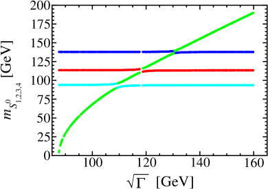
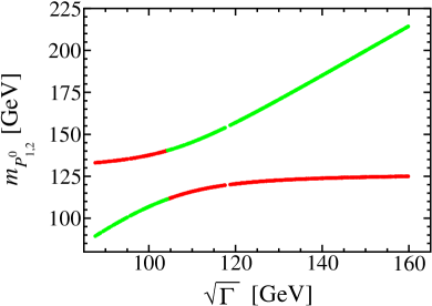
Figure 1: Typical CP-even (left) and CP-odd (right) Higgs masses as function of the parameter $\Gamma$. In this example there are four light CP-even states and two light massive CP-odd states (plus two massless states, $G^{0}$ and $J$, not shown). Just as in the MSSM there is always one light doublet state, coinciding with $h^{0}$ in the limit of zero mixing. Other states can (but need not) be light, depending on the parameters $\Omega$ and $\Gamma$, see text.

The model clearly exhibits decoupling, just as the MSSM. In the limit where $\Omega$ goes to infinity the masses of both states $P_{A^{0}}$ and $S_{H^{0}}$ go to infinity, just as what happens in the MSSM when $m_{A^{0}}$ goes to infinity. The states $S_{J_{\perp}}$ and $P_{J_{\perp}}$ are decoupled in the limit as $\Gamma$ goes to infinity. If, in addition, we require $h\ll 1$ also $S_{J}$ decouples and the SM Higgs phenomenology is recovered, as in the MSSM.

IV Higgs boson production

Supersymmetric Higgs bosons can be produced at an $e^{+}e^{-}$ collider through their couplings to $Z^{0}$, via the so–called Bjorken process ($e^{+}e^{-}\rightarrow Z^{0}S^{0}_{i}$), or via the associated production mechanism ($e^{+}e^{-}\rightarrow S^{0}_{i}P^{0}_{j}$). In our SBRP model there are 8 neutral CP-even states $S^{0}_{i}$ and 6 massive neutral CP-odd Higgs bosons $P^{0}_{i}$, in addition to the majoron $J$ and the Goldstone $G^{0}$, see Eq. (11).

One must diagonalize the (pseudo-)scalar boson mass matrices in order to find the couplings of the scalars to the $Z^{0}$. After doing that we obtain the Lagrangian terms

$${\cal L}\supset\sum_{i=1}^{8}(\sqrt{2}G_{F})^{1/2}M_{Z}^{2}Z^{0}_{\mu}Z^{0\mu}\,\eta_{{\rm B}_{i}}S^{0}_{i}+\sum_{i,j=1}^{8}(\sqrt{2}G_{F})^{1/2}M_{Z}\,\eta_{{\rm A}_{ij}}\left(Z^{0\mu}S^{0}_{i}\overleftrightarrow{\partial_{\mu}}P^{0}_{j}\right)$$ (36)

with each $\eta_{{\rm B}_{i}}$ given as a weighted combination of the five SU(2) $\otimes$ U(1) doublet scalars,

$$\eta_{{\rm B}_{i}}=\frac{v_{d}}{v}R^{S^{0}}_{i1}+\frac{v_{u}}{v}R^{S^{0}}_{i2}+\sum_{j=1}^{3}\frac{v_{Lj}}{v}R^{S^{0}}_{ij+2}$$ (37)

and the $\eta_{{\rm A}_{ij}}$ given by

$$\eta_{{\rm A}_{ij}}=R^{S^{0}}_{i1}R^{P^{0}}_{j1}-R^{S^{0}}_{i2}R^{P^{0}}_{j2}+\sum_{k=1}^{3}R^{S^{0}}_{ik+2}R^{P^{0}}_{jk+2}$$ (38)

where the subscripts ${\rm B}$ and ${\rm A}$ refer, respectively, to the Bjorken process or associated production mechanisms. From these Lagrangian terms we can easily derive the production cross sections. These are simple generalizations of the MSSM results Accomando:1997wt ; pocsik:1981bg and for completeness we give them in Appendix A.

In the MSSM, there are two sum rule rules, one concerning only the CP even sector

$$\eta_{{\rm B}_{h^{0}}}^{2}+\eta_{{\rm B}_{H^{0}}}^{2}=1\,,$$ (39)

and another relating the Bjorken and the associated production mechanisms,

$$\eta_{{\rm B}_{h^{0}}}^{2}+\eta_{{\rm A}_{h^{0}A^{0}}}^{2}=1\,,$$ (40)

with $\eta_{{\rm B}_{h^{0}}}=\sin(\alpha-\beta)$ and $\eta_{{\rm A}_{h^{0}A^{0}}}=\eta_{{\rm B}_{H^{0}}}=\cos(\alpha-\beta)$, in an obvious notation.

It is very easy, and instructive, to use our expressions for $\eta_{\rm A}$ and $\eta_{\rm B}$ to recover the MSSM result in the limit that we have only the $H_{d}$ and $H_{u}$ doublets. In fact, in this case

$$\frac{v_{d}}{v}=R^{P^{0}}_{22}\,,\qquad\frac{v_{u}}{v}=R^{P^{0}}_{21}\,,$$ (41)

so we have

$$\eta_{{\rm B}_{h^{0}}}=R^{P^{0}}_{22}R^{S^{0}}_{11}+R^{P^{0}}_{21}R^{S^{0}}_{12}\,,\quad\eta_{{\rm B}_{H^{0}}}=R^{P^{0}}_{22}R^{S^{0}}_{21}+R^{P^{0}}_{21}R^{S^{0}}_{22}\,,\quad\eta_{{\rm A}_{h^{0}A^{0}}}=R^{P^{0}}_{21}R^{S^{0}}_{11}-R^{P^{0}}_{22}R^{S^{0}}_{12}$$ (42)

and we get for the sum rule of Eq. (40)

$$\eta_{{\rm A}_{h^{0}A^{0}}}^{2}+\eta_{{\rm B}_{h^{0}}}^{2} = \left(R^{P^{0}}_{22}R^{S^{0}}_{11}+R^{P^{0}}_{21}R^{S^{0}}_{12}\right)^{2}+\left(R^{P^{0}}_{21}R^{S^{0}}_{11}-R^{P^{0}}_{22}R^{S^{0}}_{12}\right)^{2}$$ (43)

$$= \left(R^{S^{0}}_{11}R^{S^{0}}_{11}+R^{S^{0}}_{12}R^{S^{0}}_{12}\right)\left(R^{P^{0}}_{21}R^{P^{0}}_{21}+R^{P^{0}}_{22}R^{P^{0}}_{22}\right)$$ (44)

$$= 1\,,$$ (45)

where we have used the orthogonality of the rotation matrices

$$\sum_{k=1}^{2}R^{S^{0}}_{ik}R^{S^{0}}_{jk}=\delta_{ij}\,,\quad\sum_{k=1}^{2}R^{P^{0}}_{ik}R^{P^{0}}_{jk}=\delta_{ij}\,,\quad(i,j=1,2)\,.$$ (46)

For the sum rule of the CP-even sector, Eq. (39), we get

$$\eta_{{\rm B}_{h^{0}}}^{2}+\eta_{{\rm B}_{H^{0}}}^{2} = \cos^{2}\beta\left(R^{S^{0}}_{11}R^{S^{0}}_{11}+R^{S^{0}}_{21}R^{S^{0}}_{21}\right)+\sin^{2}\beta\left(R^{S^{0}}_{12}R^{S^{0}}_{12}+R^{S^{0}}_{22}R^{S^{0}}_{22}\right)$$ (48)

$$+2\sin\beta\cos\beta\left(R^{S^{0}}_{11}R^{S^{0}}_{12}+R^{S^{0}}_{21}R^{S^{0}}_{22}\right)$$

$$= 1\,,$$ (49)

using the result that in an orthogonal matrix also the vectors corresponding to the columns are orthonormal, that is

$$\sum_{k=1}^{2}R^{S^{0}}_{ki}R^{S^{0}}_{kj}=\delta_{ij}\,,\quad(i,j=1,2)\,.$$ (50)

How this differs in our case? The difference is that, in general,

$$\sum_{k=1}^{2}R^{S^{0},P^{0}}_{ik}R^{S^{0},P^{0}}_{jk}\not=\delta_{ij}\quad\hbox{and}\quad\sum_{k=1}^{2}R^{S^{0},P^{0}}_{ki}R^{S^{0},P^{0}}_{kj}\not=\delta_{ij}\,,$$ (51)

due to the fact that we now have more than two (pseudo-)scalars. As it was stated in the last section and will be discussed in more detail when we consider the decays, to have a sizeable invisible branching ratio we need the doublets to be close in mass to the singlet states related to the majoron and orthogonal combinations. This means that, in the CP-even sector, the first four states are $(S_{h^{0}},S_{H^{0}},S_{J_{\perp}},S_{J})$, while in the CP-odd sector we should have $(P_{A_{0}},P_{J_{\perp}},J,G^{0})$. If this situation happens then we can very easily find a generalization of the sum rule of the CP-even sector, as

$$\eta_{{\rm B}_{S_{h^{0}}}}^{2}+\eta_{{\rm B}_{S_{H^{0}}}}^{2}+\eta_{{\rm B}_{S_{J_{\perp}}}}^{2}+\eta_{{\rm B}_{S_{J}}}^{2}=1$$ (52)

to a good approximation. This is displayed in Fig. 2 where we plot the sum $\eta_{{\rm B}_{S_{H^{0}}}}^{2}+\eta_{{\rm B}_{S_{J_{\perp}}}}^{2}+\eta_{{\rm B}_{S_{J}}}^{2}$ against $\eta_{{\rm B}_{S_{h^{0}}}}^{2}$.

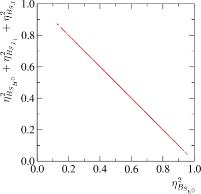
Figure 2: Sum rule in the CP-even sector, for the case explained in the text. The four states, $(S_{h^{0}},S_{H^{0}},S_{J_{\perp}},S_{J})$. For this example all scalar masses are taken below $200$ GeV.

The significance of this sum rule should be clear: if the lightest Higgs boson has a very small coupling to the $Z^{0}$ and hence a small production cross section, there should be another state nearby that has a large production cross section.

The other sum rule, relating the CP-even and CP-odd sectors, Eq. (40), is more difficult to generalize. In fact the $P_{A_{0}}$ state will now mix with the $P_{J_{\perp}}$ and the identification of Eq. (41) will be no longer true. However qualitatively the sum rule still holds in the sense that if the parameters are such that the production of the CP-odd states is reduced one always gets a CP-even state produced.

The above discussion has concentrated on Higgs boson production at an $e^{+}e^{-}$ collider. We now briefly comment on the differences with regards to Higgs production at the LHC Romao:1992dc . It has been suggested to search for an invisibly decaying Higgs at the LHC in $WW$ boson fusion Eboli:2000ze , in asociated production with a $Z^{0}$ boson Godbole:2003it , or in the $t{\bar{t}}$ channel Gunion:1993jf . For the production in $WW$ fusion or in asociated production with a $Z^{0}$ boson the above discussion applies straightforwardly, since the relevant coupling in both cases is $\eta_{B_{i}}$ (i.e. $sin(\beta-\alpha)$ in the MSSM limit). For the $t{\bar{t}}$ channel in the MSSM production cross section the factor $\cos\alpha$ has to be replaced by $R^{S^{0}}_{i2}$ for the SBRP model.

V Higgs boson decays

In the following we will discuss the decays of light CP-even and CP-odd supersymmetric Higgs bosons. Since the phenomenology of Higgs bosons within the MSSM is well-known hunters ; gunion:1986yn , we will concentrate on non-standard final states. Of these, the most important are the majoron Higgs boson decay modes, which are characteristic of the SBRP model, without an MSSM counterpart. We will limit ourselves to the discussion of light states, i.e. Higgs bosons with masses below the $2W$ threshold. As discussed below, the decays of heavier CP-odd states will be similar to the situation encountered in the (N)MSSM.

V.1 CP-even Higgs Boson Decays

In the MSSM light CP-even Higgs bosons decay dominantly to $b{\bar{b}}$ final states. In our calculation we take into account all fermion final states, including the leading QCD radiative corrections from Djouadi:1995gt . In the SBRP model new decay modes appear, such as $S^{0}_{i}\to JJ$ and, if kinematically allowed $S^{0}_{i}\to P^{0}_{j}J$ and $S^{0}_{i}\to P^{0}_{j}P^{0}_{k}$. From the latter usually only $S^{0}_{i}\to JJ$ has a large branching ratio (see appendix B).

In Ref. Hirsch:2004rw we have discussed the invisible decays of the lightest CP-even Higgs boson. We now extend that discussion so as to include also the next-to-lightest CP-even state which plays an important role, if the lightest CP-even state is mainly singlet.

It is well known that, in contrast to the Standard Model, in the MSSM (and in the NMSSM) the mass of the lightest CP-even supersymmetric Higgs boson obeys an upper bound that follows from the D-term origin of the quartic terms in the scalar potential, contained in Eq. (II). This mass acquires a contribution from the top-stop quark exchange haber:1991aw ; ellis:1991zd ; Okada:1990vk , a fact that modifies the numerical value of this upper bound haber:1991aw ; ellis:1991zd ; Okada:1990vk . Many other loops contribute, for a recent two-loop level calculation see, e.g. Ref. heinemeyer:1998np . This limit is slightly relaxed in the NMSSM as opposed to the MSSM ellwanger:1999ji .

How does this bound emerge in the SBRP model? Since the CP-even sector contains eight scalars, we cannot diagonalize the corresponding mass matrices analytically. Therefore we calculate the upper bound on the Higgs mass numerically, and including the most important radiative corrections, using formulas from ellis:1991zd . In the SBRP model it is possible that the lightest CP-even Higgs is mainly a singlet. However, if this happens, there must exist a light, mainly doublet Higgs, to which the NMSSM bounds apply. This is shown in Fig. 3, where we plot (to the left) $\eta_{{\rm B}_{2}}^{2}$ as function of the $\eta_{{\rm B}_{1}}^{2}$ and (to the right) the upper limit on the mass of the second lightest Higgs as function of $\eta_{{\rm B}_{2}}^{2}$. As is seen, if the lightest state is mainly singlet, $\eta_{{\rm B}_{1}}^{2}\simeq 0$, therefore $\eta_{{\rm B}_{2}}^{2}\simeq 1$, then there is an upper bound on the second lightest state mass. Vice versa the upper bound applies to the lightest state if it is mainly doublet.

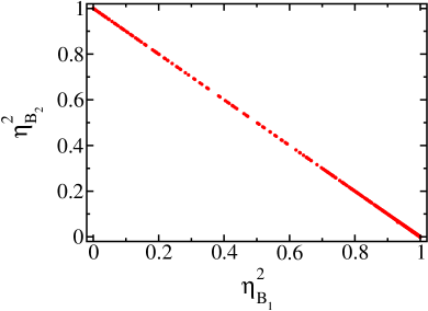
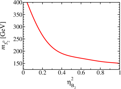
Figure 3: In the left panel we show the parameter characterizing direct production of the second lightest neutral CP-even Higgs boson, $\eta_{{\rm B}_{2}}^{2}$, as function of the corresponding one for the first lightest neutral CP-even Higgs boson, $\eta_{{\rm B}_{1}}^{2}$. To the right: Upper limit on the mass of the second lightest CP-even Higgs as a function of $\eta_{{\rm B}_{2}}^{2}$.

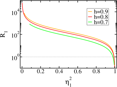
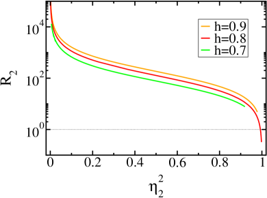
Figure 4: To the left (right): Ratio $R_{1}$ ($R_{2}$) as a function of the direct production parameter, $\eta_{{\rm B}_{1}}^{2}$ ($\eta_{{\rm B}_{2}}^{2}$), for the first (second) lightest neutral CP-even Higgs boson.

As shown previously Hirsch:2004rw , one can have large direct production cross section for the lightest neutral CP-even Higgs boson as well as a large branching ratio to the invisible final majoron states. This is demonstrated in the left panel of Fig. 4 for a random but fixed choice of undisplayed parameters. We note that a very similar behaviour is also found for the second lightest state, as seen from the right panel of Fig. 4. Thus if the lightest state is mainly singlet there must be a state nearby which is mainly doublet and decays invisibly.

In summary, we have seen that in the SBRP model there is always at least one light state, which is mainly doublet, and therefore can be produced at future colliders. Irrespectively of whether this state is the lightest or second-lightest Higgs state, it can decay with very large branching ratio to an invisible final state.

V.2 CP-odd Higgs Boson Decays

Light CP-odd Higgs bosons in the MSSM decay according to $P^{0}_{i}\to f{\bar{f}}$. The $WW$ channel becomes dominant as soon as kinematically allowed hunters ; gunion:1986yn , however we will not include it as we are mainly interested in the possibility of invisible decays of the lowest-lying pseudoscalar. The formulas for the CP-even and CP-odd Higgs boson MSSM decay branching ratios, apart from the larger number of Higgs bosons, are totally analogous to those of the MSSM Djouadi:1995gt , except for the prefactors which are determined by the diagonalizing matrices of our model. The corresponding matrix elements replace the familiar $\sin(\beta-\alpha)$ and $\cos(\beta-\alpha)$ factors.

In the SBRP we must take into account in addition the decays $P^{0}_{i}\to JJJ$ and, if kinematically allowed, also $P^{0}_{i}\to S^{0}_{j}J$, $P^{0}_{i}\to S^{0}_{j}P^{0}_{k}$, $P^{0}_{i}\to P^{0}_{j}JJ$, $P^{0}_{i}\to P^{0}_{j}P^{0}_{k}J$ and $P^{0}_{i}\to P^{0}_{j}P^{0}_{k}P^{0}_{m}$. For the lightest Higgs boson we are interested only in $P^{0}_{i}\to JJJ$ and $P^{0}_{i}\to S^{0}_{j}J$. The formulas for the CP-even and CP-odd Higgs boson non-MSSM decay widths are collected in appendix B.

V.3 $P^{0}_{i}\to S^{0}_{j}J$

The decay width of the CP-odd Higgs boson to a CP-even Higgs boson and a majoron is given in Eq. (63). Using the approximation Eq. (10) we can find the coupling $g^{\prime}_{ij}$ for the vertex $S^{\prime 0}_{i}P^{\prime 0}_{j}J$ of the majoron with the unrotated neutral scalar $S^{\prime 0}_{i}$ and pseudoscalar $P^{\prime 0}_{j}$ to leading order in the small parameter $\frac{v_{L}}{v}$ as

$$g^{\prime}_{11} = \frac{g^{2}+g^{\prime 2}}{4}\;\frac{v_{d}^{2}v_{L}^{2}}{Vv^{2}}\,,$$

$$g^{\prime}_{12} = \left(\frac{g^{2}+g^{\prime 2}}{4}-h_{0}^{2}\right)\frac{v_{d}v_{u}v_{L}^{2}}{Vv^{2}}\,,$$

$$g^{\prime}_{21} = -\left(\frac{g^{2}+g^{\prime 2}}{4}-h_{0}^{2}\right)\frac{v_{d}v_{u}v_{L}^{2}}{Vv^{2}}\,,$$

$$g^{\prime}_{22} = -\frac{g^{2}+g^{\prime 2}}{4}\;\frac{v_{u}^{2}v_{L}^{2}}{Vv^{2}}\,,$$

$$g^{\prime}_{i1} = \frac{-\mu\epsilon_{i-2}}{V}\qquad(i=3,\ldots,5)\,,$$

$$g^{\prime}_{i2} = \frac{-\epsilon_{i-2}}{V}\left(A_{h_{\nu}}+\frac{v_{S}}{v_{R}}\hat{M}_{R}\right)\qquad(i=3,\ldots,5)\,,$$

$$g^{\prime}_{61} = \frac{v_{L}^{2}}{v^{2}V}\left(\sqrt{2}h_{0}\mu v_{d}-\frac{1}{\sqrt{2}}\left(h_{0}\hat{M}_{\Phi}+A_{h_{0}}\right)v_{u}\right)\,,$$

$$g^{\prime}_{62} = \frac{v_{L}^{2}}{v^{2}V}\left(-\sqrt{2}h_{0}\mu v_{u}+\frac{1}{\sqrt{2}}\left(h_{0}\hat{M}_{\Phi}+A_{h_{0}}\right)v_{d}\right)\,,$$

$$g^{\prime}_{71} = \frac{-hh_{0}v_{u}v_{R}}{2V}\,,$$

$$g^{\prime}_{72} = \frac{-hh_{0}v_{d}v_{R}}{2V}\,,$$

$$g^{\prime}_{81} = \frac{hh_{0}v_{u}v_{S}}{2V}\,,$$

$$g^{\prime}_{82} = \frac{hh_{0}v_{d}v_{S}}{2V}\,.$$ (53)

Note that the first four of the above are suppressed by the smallness of sneutrino vevs, needed to reproduce the observed neutrino oscillation data. The coupling $g_{S^{0}_{i}P^{0}_{j}J}$ then appears through mixing, and is given as

$$g_{S^{0}_{i}P^{0}_{j}J}=g^{\prime}_{71}R^{S^{0}}_{i7}R^{P^{0}}_{j1}+g^{\prime}_{72}R^{S^{0}}_{i7}R^{P^{0}}_{j2}+g^{\prime}_{81}R^{S^{0}}_{i8}R^{P^{0}}_{j1}+g^{\prime}_{82}R^{S^{0}}_{i8}R^{P^{0}}_{j2}\,.$$ (54)

V.4 $P^{0}_{i}\to JJJ$

The decay width of the CP-odd Higgs boson to three majorons is given in Eq. (66). Using again the approximate equation giving the profile of the majoron, Eq. (10), the coupling $g^{\prime}_{i}$ for the vertex $P^{\prime 0}_{i}JJJ$ of the majorons with the unrotated neutral pseudoscalar $P^{\prime 0}_{i}$, is given as

$$g^{\prime}_{1} = -\frac{3v_{L}^{2}}{v^{2}V^{3}}h_{0}hv_{u}v_{R}v_{S}\,,$$

$$g^{\prime}_{2} = \frac{3v_{L}^{2}}{v^{2}V^{3}}h_{0}hv_{d}v_{R}v_{S}\,,$$

$$g^{\prime}_{3} \sim g^{\prime}_{4}\sim g^{\prime}_{5}\sim{\cal O}(\frac{v_{L}^{3}}{v^{3}})\,,$$

$$g^{\prime}_{6} \sim {\cal O}(\frac{v_{L}^{3}\epsilon}{v^{3}V})\,,$$

$$g^{\prime}_{7} = \frac{-3h^{2}v_{S}v_{R}^{2}}{V^{3}}\,,$$

$$g^{\prime}_{8} = \frac{3h^{2}v_{S}^{2}v_{R}}{V^{3}}\,.$$ (55)

Again, the first six of the above vanish in the limit $v_{L}\to 0$. Therefore the coupling $g_{P^{0}_{i}JJJ}$ for the vertex of the majorons with the neutral pseudoscalar $P^{0}_{i}$ mass eigenstate is

$$g_{P^{0}_{i}JJJ}=g^{\prime}_{7}R^{P^{0}}_{i7}+g^{\prime}_{8}R^{P^{0}}_{i8}.$$ (56)

V.5 Numerical results

We can see from Eq. (V.3) that if the CP-odd mass eigenstate is mainly a Higgs doublet (i.e., its main components are $P^{\prime 0}_{1}=H_{d}^{0I},\;P^{\prime 0}_{2}=H_{u}^{0I}$ so that its production is not reduced) then its decays to $S^{0}_{j}J$ and $JJJ$ are suppressed as the corresponding couplings are very small, suppressed by two powers in $\frac{v_{L}}{v}$. To find sizeable branching ratios for the decays of the lightest massive pseudoscalar $P^{0}_{1}$, mixing between doublet and singlet states is therefore required.

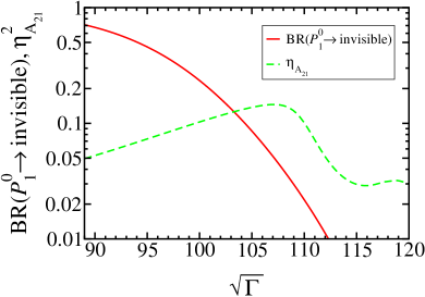
Figure 5: Production cross section (red/solid curve) and invisible final states decay branching ratio (green/dashed curve) for the lightest CP-odd Higgs boson.

As discussed in section III, in order to have sizeable mixing between doublet and singlet CP-odd Higgs bosons, we must require that at least one of the singlet states is light, i.e. the parameter $\Gamma$ should be very roughly of order $\Gamma\sim\Omega$. Fig. 5 shows an example. Here, we plot $\eta^{2}_{{\rm A}_{21}}$ and ${\rm BR}(P^{0}_{1}\to\hskip 2.84526pt{\rm inv})$ as function of $\sqrt{\Gamma}$ for one fixed, but arbitrary set of other model parameters. For small values of $\sqrt{\Gamma}$ the lightest massive CP-odd state is mainly singlet, therefore ${\rm BR}(P^{0}_{1}\to\hskip 2.84526pt{\rm inv})$ is close to 1. However, the production parameter $\eta^{2}_{{\rm A}_{21}}$ is small. Increasing $\sqrt{\Gamma}$ increases the mass of the lightest CP-odd state. From a certain point onwards, it is the doublet state which is lightest, compare to Fig. 1. This state can have a sizeable production, but the branching ratio to invisible final states typically is small. Only in the intermediate region of sizeable mixing between doublet and singlet states, i.e. in the region of $\sqrt{\Gamma}\sim 100-115$ GeV of Fig. 5 one can have both, sizeable production and sizeable invisible decay.

In summary, the CP-odd Higgs bosons in the SBRP model usually behave very similar to the situation discussed in the (N)MSSM. However, sizeable branching ratios to invisible final states are possible when there are light CP-odd Higgs bosons from both, the doublet and the singlet sectors.

VI Discussion

We have carefully analyzed the mass spectra, production and decay properties of the lightest supersymmetric CP-even and CP-odd Higgs bosons in models with spontaneously broken R-parity. We have compared the resulting mass spectra with what is predicted in the Minimal Supersymmetric Standard Model, stressing the validity of the upper bound on the lightest CP-even Higgs boson mass. We have seen how the presence of the additional scalar singlet states affects the Higgs production cross sections, both in the Bjorken and associated modes.

The main difference with respect to the MSSM case comes from the fact that the spontaneous breaking of lepton number necessarily implies the existence of the majoron, and this opens new decay channels for supersymmetric Higgs bosons into “invisible” final states. We have found that the invisible decays of CP-even Higgses can be dominant, despite the small values of the neutrino masses indicated by neutrino oscillation data. In contrast, although the decays of the CP-odd bosons into invisible final states can also be sizeable, this situation is not generic.

Therefore the existence of invisibly decaying Higgs bosons should be taken seriosly in the planning of future accelerators, like the LHC and the ILC. These decays may signal the weak-scale violation of lepton number in a wide class of theories. Within the supersymmetric context they are a characteristic feature of the SBRP models. These can account for the observed pattern of neutrino masses and mixings in a way which allows the neutrino mixing angles to be cross checked at high energy accelerators like LHC/ILC. For example, in our model there is a $b{\bar{b}}$ plus missing momentum signal associated to the invisible decay of the lightest CP-even Higgs boson produced in association with a pseudoscalar. Although this is a standard topology, also present in the Standard Model and the MSSM, its kinematical properties in our model differ, as the $JJ$ add up to the CP-even Higgs boson mass and $b{\bar{b}}$ to the CP-odd Higgs boson mass. Further studies to elucidate the impact of these decay modes for future colliders, should be conducted. While for the LHC we may encounter difficulties associated to missing energy measurements and/or b-tagging, these potential limitations do not affect in the same way the ILC.

Last, but not least, as already explained, we have restricted our analysis to Higgs bosons below the $WW$ threshold. Extension to relax this restriction is totally straightforward, though somewhat less interesting. Due to the validity of the supersymmetric Higgs boson mass upper limit we must have one light CP-even Higgs boson which, as we have shown, is likely to have an important decay into invisible final states.

Appendix A Production cross sections

In this section we give the formulas for the production cross section of both channels at an $e^{+}e^{-}$ machine.

A.1 Bjorken process

The cross section for the Bjorken process is Accomando:1997wt

$$\sigma(e^{+}e^{-}\to Z^{0}S^{0}_{i})=\eta_{{\rm B}_{i}}^{2}\ \frac{G_{F}^{2}M_{Z}^{4}}{96\pi s}\,\left(v_{e}^{2}+a_{e}^{2}\right)\,\beta\frac{\beta^{2}+12M_{Z}^{2}/s}{(1-M_{Z}^{2}/s)^{2}+\left(\Gamma_{Z}M_{Z}/s\right)^{2}}\,,$$ (57)

where

$$v_{e}=-1+4\sin\theta_{W}^{2},\ a_{e}=-1,\quad\beta=\frac{\lambda(s,M_{Z}^{2},M_{S^{0}_{i}}^{2})}{s}\ ,$$ (58)

$\lambda$ is the 2-body phase space function,

$$\lambda(a,b,c)=\sqrt{\left(a+b-c\right)^{2}-4ab}$$ (59)

and the $\eta_{{\rm B}_{i}}$ are given in Eq. (37).

A.2 Associated production

The cross section for the associated production is pocsik:1981bg

$$\sigma(e^{+}e^{-}\to S^{0}_{i}P^{0}_{j})=\eta_{{\rm A}_{ij}}^{2}\ \frac{G_{F}^{2}M_{Z}^{4}}{96\pi s}\,\left(v_{e}^{2}+a_{e}^{2}\right)\,\frac{\beta^{3}}{(1-M_{Z}^{2}/s)^{2}+\left(\Gamma_{Z}M_{Z}/s\right)^{2}}$$ (60)

with

$$\beta=\frac{\lambda(s,M_{P^{0}_{j}}^{2},M_{S^{0}_{i}}^{2})}{s}$$ (61)

and the $\eta_{{\rm A}_{ij}}$ are given in Eq. (38).

Appendix B Non-MSSM decays

The most characteristic decays of this model which do not exist in the (N)MSSM are those involving a majoron. In the following we collect the formulas for these decays. The most important ones are:

$$\Gamma(S^{0}_{i}\to JJ)=\frac{g_{S^{0}_{i}JJ}^{2}}{32\pi m_{S^{0}_{i}}}\,,$$ (63)

$$\Gamma(P^{0}_{i}\to S^{0}_{j}J)=\frac{g_{S^{0}_{j}P^{0}_{i}J}^{2}}{16\pi m_{P^{0}_{i}}^{3}}\left(m_{P^{0}_{i}}^{2}-m_{S^{0}_{j}}^{2}\right)\,.$$

For completeness we consider also:

$$\Gamma(S^{0}_{i}\to P^{0}_{j}J)=\frac{g_{S^{0}_{i}P^{0}_{j}J}^{2}}{16\pi m_{S^{0}_{i}}^{3}}\left(m_{S^{0}_{i}}^{2}-m_{P^{0}_{j}}^{2}\right)\,,$$ (64)

$$\Gamma(P^{0}_{i}\to S^{0}_{j}P^{0}_{k})=\frac{g_{S^{0}_{j}P^{0}_{i}P^{0}_{k}}^{2}}{16\pi m_{P^{0}_{i}}^{3}}\lambda(m_{P^{0}_{i}}^{2},m_{S^{0}_{j}}^{2},m_{P^{0}_{k}}^{2})\,,$$ (65)

$$\Gamma(P^{0}_{i}\to JJJ)=\frac{m_{P^{0}_{i}}\,g^{2}_{P^{0}_{i}JJJ}}{3072\pi^{3}}\,,$$ (66)

$$\Gamma(P^{0}_{i}\to P^{0}_{j}JJ)=\frac{g_{P^{0}_{i}P^{0}_{j}JJ}^{2}}{1024\pi^{3}m_{P^{0}_{i}}^{3}}\left(m_{P^{0}_{i}}^{4}-m_{P^{0}_{j}}^{4}\right)\,,$$ (67)

$$\Gamma(P^{0}_{i}\to P^{0}_{j}P^{0}_{k}J)=\frac{g_{P^{0}_{i}P^{0}_{j}P^{0}_{k}J}^{2}}{512\pi^{3}m_{P^{0}_{i}}^{3}}\lambda(m_{P^{0}_{i}}^{2},m_{P^{0}_{j}}^{2},m_{P^{0}_{k}}^{2})\;\times\left\{\begin{array}[]{l}\displaystyle\frac{1}{2}\,,\quad j=k\cr 1\,,\quad j\not=k\end{array}\right\}$$ (70)

$$\hskip 14.22636pt\times\,\frac{m_{P^{0}_{i}}^{2}\left(m_{P^{0}_{i}}^{2}-2m_{P^{0}_{j}}m_{P^{0}_{k}}\right)+2m_{P^{0}_{j}}m_{P^{0}_{k}}\left(m_{P^{0}_{j}}+m_{P^{0}_{k}}\right)^{2}-\left(m_{P^{0}_{j}}+m_{P^{0}_{k}}\right)^{4}}{m_{P^{0}_{i}}^{2}-\left(m_{P^{0}_{j}}+m_{P^{0}_{k}}\right)^{2}}\,.$$ (71)

The decays $P^{0}_{i}\to P^{0}_{j}P^{0}_{k}P^{0}_{l}$ are possible, but closed kinematically for the light states of interest, therefore we do not give here the explicit formulas for the widths.

References

• (1) M. Carena and H. E. Haber, Prog. Part. Nucl. Phys. 50, 63 (2003), [hep-ph/0208209].
• (2) A. B. McDonald, New J. Phys.  6, 121 (2004) [astro-ph/0406253].
• (3) T. Kajita, New J. Phys. 6, 194 (2004).
• (4) T. Araki et al. [KamLAND Collaboration], Phys. Rev. Lett.  94, 081801 (2005) [hep-ex/0406035].
• (5) M. Maltoni, T. Schwetz, M. A. Tortola and J. W. F. Valle, New J. Phys. 6, 122 (2004), [hep-ph/0405172].
• (6) M. Hirsch and J. W. F. Valle, New J. Phys. 6, 76 (2004), [hep-ph/0405015].
• (7) M. A. Diaz, J. C. Romao and J. W. F. Valle, Nucl. Phys. B524, 23 (1998), [hep-ph/9706315].
• (8) M. Hirsch et al., Phys. Rev. D 62, 113008 (2000) [Erratum-ibid. D 65, 119901 (2002)] [hep-ph/0004115]. M. A. Diaz et al., Phys. Rev. D68, 013009 (2003), [hep-ph/0302021].
• (9) J. C. Romao et al., Phys. Rev. D61, 071703 (2000), [hep-ph/9907499].
• (10) E. J. Chun and S. K. Kang, Phys. Rev. D61, 075012 (2000), [hep-ph/9909429].
• (11) A. Abada, S. Davidson and M. Losada, Phys. Rev. D65, 075010 (2002), [hep-ph/0111332].
• (12) W. Porod, D. Restrepo and J. W. F. Valle, hep-ph/0001033; M. Hirsch and W. Porod, Phys. Rev. D68, 115007 (2003), [hep-ph/0307364]; M. Hirsch, W. Porod, J. C. Romao and J. W. F. Valle, Phys. Rev. D66, 095006 (2002), [hep-ph/0207334]; W. Porod, M. Hirsch, J. Romao and J. W. F. Valle, Phys. Rev. D63, 115004 (2001), [hep-ph/0011248]; D. Restrepo, W. Porod and J. W. F. Valle, Phys. Rev. D64, 055011 (2001), [hep-ph/0104040].
• (13) A. Masiero and J. W. F. Valle, Phys. Lett. B251, 273 (1990).
• (14) J. C. Romao, C. A. Santos and J. W. F. Valle, Phys. Lett. B288, 311 (1992).
• (15) J. C. Romao, A. Ioannisian and J. W. F. Valle, Phys. Rev. D55, 427 (1997), [hep-ph/9607401].
• (16) M. Shiraishi, I. Umemura and K. Yamamoto, Phys. Lett. B313, 89 (1993).
• (17) A. S. Joshipura and J. W. F. Valle, Nucl. Phys. B397, 105 (1993).
• (18) J. C. Romao, F. de Campos and J. W. F. Valle, Phys. Lett. B292, 329 (1992), [hep-ph/9207269].
• (19) M. Hirsch, J. C. Romao, J. W. F. Valle and A. Villanova del Moral, Phys. Rev. D70, 073012 (2004), [hep-ph/0407269].
• (20) C. Panagiotakopoulos and A. Pilaftsis, Phys. Rev. D63, 055003 (2001), [hep-ph/0008268].
• (21) A. Dedes, C. Hugonie, S. Moretti and K. Tamvakis, Phys. Rev. D63, 055009 (2001), [hep-ph/0009125].
• (22) E. Accomando et al. [ECFA/DESY LC Physics Working Group], Phys. Rept.  299, 1 (1998) [hep-ph/9705442].
• (23) G. Pocsik and G. Zsigmond, Zeit. Phys. C10, 367 (1981).
• (24) J. C. Romao, J. L. Diaz-Cruz, F. de Campos and J. W. F. Valle, Mod. Phys. Lett. A9, 817 (1994), [hep-ph/9211258].
• (25) O. J. P. Eboli and D. Zeppenfeld, Phys. Lett. B495, 147 (2000), [hep-ph/0009158].
• (26) R. M. Godbole, M. Guchait, K. Mazumdar, S. Moretti and D. P. Roy, Phys. Lett. B571, 184 (2003), [hep-ph/0304137].
• (27) J. F. Gunion, Phys. Rev. Lett. 72, 199 (1994), [hep-ph/9309216].
• (28) J. Gunion, H. Haber, G. Kane and S. Dawson, The Higgs Hunter’s Guide, Frontiers in Physics (Westview Press, Boulder, Colorado, 1990).
• (29) J. F. Gunion and H. E. Haber, Nucl. Phys. B272, 1 (1986).
• (30) A. Djouadi, M. Spira and P. M. Zerwas, Z. Phys. C70, 427 (1996), [hep-ph/9511344].
• (31) H. E. Haber and R. Hempfling, Phys. Rev. Lett. 66, 1815 (1991).
• (32) J. R. Ellis, G. Ridolfi and F. Zwirner, Phys. Lett. B262, 477 (1991).
• (33) Y. Okada, M. Yamaguchi and T. Yanagida, Prog. Theor. Phys. 85, 1 (1991).
• (34) S. Heinemeyer, W. Hollik and G. Weiglein, Eur. Phys. J. C9, 343 (1999), [hep-ph/9812472].
• (35) U. Ellwanger and C. Hugonie, Eur. Phys. J. C25, 297 (2002), [hep-ph/9909260].