Chiral phase transition in effective models of QCD

Abstract:

Incorporating its most relevant global symmetry, chiral effective models are aimed at investigating, in a simplified framework, important aspects of the yet unsolved QCD. We review some recent results obtained in these models on the restoration of chiral and axial symmetries, on the boundary of the first order phase transition region in the $m_{\pi}-m_{K}$–plane at vanishing baryonic chemical potential $\mu_{B}$, and on the $\mu_{B}-T$ phase diagram.

1 Introduction

Although the issue of the deconfinement phase transition in strongly interacting matter can be addressed with first principle calculation in lattice field theory, it is of interest to see what can be obtained regarding the chiral symmetry restoration aspect of the transition within effective models sharing the same global symmetry as QCD. For vanishing chemical potential universality classes of the transitions of strongly interacting matter were predicted by effective models for three corners of the $m_{u,d}-m_{s}$–plane: the exact SU(3) chiral limit ($m_{u,d,s}=0$), the two flavor chiral case ($m_{u,d}=0,$ $m_{s}=\infty$) and the pure gauge theory ($m_{u,d,s}=\infty$). As a consequence of the compatibility of the conclusions there has to be also a tricritical point (TCP) on the $m_{u,d}=0$ line [1]. Apart from these corners and $m_{u,d}=0$ axis no universal arguments exist and the order of the transition for different values of the chemical potentials (baryonic, isospin) and quark masses, as well as the shape of the transition line between regions of crossover and first order transitions are a matter of calculation.

It is expected that at vanishing baryonic chemical potential for low values of the masses there is a line of second order phase transitions as a boundary of the first order phase transition region. Increasing the value of $\mu_{B}$ the second order line sweeps along a critical surface. Theoretically it is important to map the phase-diagram as a function of the parameters of QCD, and also there can be experimentally accessible interesting points, like the critical end point (CEP) occurring at finite $\mu_{B}$, for physical values of the quark masses.

Apart from helping the mapping out of the QCD phase transition, the effective models can give insights in the interplay between chiral and $U_{A}(1)$ symmetry restoration, and how meson and baryon properties change during the chiral transition. They can tell us what is the soft mode at the CEP, and by predicting specific signatures they might help finding its actual location [2]. They can also give information on the non-equilibrium dynamics near TCP or CEP [3, 4].

Effective models play also an important role whenever particle physics is applied to cosmological or astrophysical studies. In cosmology, it is in important to know what the cold dark matter is made of. The relic density of one of the candidates, the weakly interacting massive particles (WIMPs), depends on the variation of the number of relativistic degrees of freedom and the energy density of the universe. It was shown in [5] that if WIMPs freeze out in the range of the QCD transition temperature the prediction of their relic concentration depends on the QCD equation of state, which below $T_{c}$ is taken from an effective model. In astrophysics the structure of compact stars is actively investigated due to increasingly available new data that indirectly provides information on the state of matter in their core. At present effective models are the only tools for determining the equation of state of strongly interacting matter at very low temperature and high density.

In the present article a brief overview of some of the effective models will be given, and then some recent results on the issues enumerated in the Abstract will be summarised.

2 Effective chiral models

A common feature of the effective models is that they are constructed using the global chiral symmetry of the massless QCD and its spontaneous symmetry breaking pattern $SU_{L}(3)\times SU_{R}(3)\rightarrow SU_{V}(3)$. For equal quark-masses the four-divergence of the vector current vanishes, while the divergence of the axial vector current vanishes only in the massless case:

$$\partial_{\mu}\big{[}\bar{q}\gamma^{\mu}\lambda^{a}q\big{]} = i\bar{q}[M,\lambda^{a}]q=\bar{q}_{i}(m_{i}-m_{j})\lambda^{a}_{ij}q_{j},$$ (1)

$$\partial_{\mu}\big{[}\bar{q}\gamma^{\mu}\gamma_{5}\lambda^{a}q\big{]} = i\bar{q}\{\lambda^{a},M\}\gamma_{5}q=\bar{q}_{i}(m_{i}+m_{j})\lambda^{a}_{ij}\gamma_{5}q_{j},$$

where for three flavors $M=\mbox{diag}(m_{u},m_{d},m_{s})$ and there is an order parameter (OP), the chiral condensate $\displaystyle\langle 0|[Q^{a}_{A},\bar{q}\gamma_{5}\lambda^{b}q]|0\rangle=-{1\over 2}\langle 0|\bar{q}\{\lambda^{a},\lambda^{b}\}q|0\rangle=-{2\over 3}\delta_{ab}\langle 0|\bar{q}q|0\rangle$, which when vanishes indicates the restoration of chiral symmetry.

The Lagrangian contains explicit symmetry breaking terms of two kinds. One is the quark mass term, or in the linear sigma model the term containing the external sources, which gives mass to the pseudo-Goldstone bosons. The other type is the instanton motivated ’t Hooft determinant which breaks the $U_{A}(1)$ symmetry.

The effective models are built upon mesons and/or baryons with the lowest mass and are expected to be most relevant in case of a crossover transition when the mesons are well defined degrees of freedom even above the pseudo-critical temperature or in case of a second order phase transition where the change of the order parameter is directly accessible.

The effective models differ essentially from QCD in that they miss the mechanism for confinement and incorporate only the degrees of freedom thought to be relevant for the chiral transition. Because of this latter feature it is very important to have a faithful, fine-tuned parametrisation of any effective model. I mention, however, that recently there have been studies [6], [7] that included confinement in chiral models through an effective potential constructed with its (approximate) order parameter, the Polyakov loop, in an attempt to give account of the lattice result which shows that both chiral and deconfinement transitions happen at about the same temperature [8].

The chiral perturbation theory–ChPT

Chiral perturbation theory [9] describes exactly the low energy dynamics of the Goldstone particles collected in a hermitian traceless matrix $\Phi(x)$:

$$\Phi(x)=\begin{pmatrix}{\pi^{0}/\sqrt{2}}+{\eta_{8}/\sqrt{6}}&\pi^{+}&K^{+}\cr\pi^{-}&-{\pi^{0}/\sqrt{2}}+{\eta_{8}/\sqrt{6}}&K^{0}\cr K^{-}&\bar{K}^{0}&-{2\eta_{8}/\sqrt{6}}\end{pmatrix}.$$ (2)

The most general Lagrangian invariant under $SU_{L}(3)\times SU_{R}(3)$ chiral symmetry is written down in terms of the exponential of $\Phi$, $U(\Phi)=e^{i\sqrt{2}\Phi/f}$ and appears as a systematic expansion in momenta and quark masses:

$${\cal L}^{SU(3)}_{\mathrm{ChPT}}(U)=\sum_{n}{\cal L}_{2n}={f^{2}\over 4}\mbox{Tr}(\partial_{\mu}U^{\dagger}\partial^{\mu}U)+\frac{f^{2}B_{0}}{2}\mbox{Tr}(MU^{\dagger}+UM^{\dagger})+{\mathcal{O}}(p^{4}).$$ (3)

In the general $U_{L}(3)\times U_{R}(3)$ case [10] this is more complicated because each term of (3) can be multiplied by some function of $\eta_{0}=-if\log\mbox{det}U/\sqrt{6}$ (in this case $U=e^{i(\sqrt{2}\Phi+\eta_{0}\lambda^{0})/f}$). What is important for us from the point of view of the parametrisation of the linear sigma model in the $m_{\pi}-m_{K}$–plane is that ChPT determines the $m_{\pi}$ and $m_{K}$ dependence of the decay constants for pions ($f_{\pi}$) and the kaons ($f_{K}$) as well as of $M_{\eta}^{2}=m_{\eta}^{2}+m_{\eta^{\prime}}^{2}$:

$$f_{\pi} = f\left[1-\frac{1}{f^{2}}(2\mu_{\pi}+\mu_{K}-4m_{\pi}^{2}(L_{4}+L_{5})-8m_{K}^{2}L_{4})\right],$$ (4)

$$f_{K} = f\left[1-\frac{1}{f^{2}}\left(\frac{3}{4}(\mu_{\pi}+\mu_{\eta}+2\mu_{K})-4m_{\pi}^{2}L_{4}-4m_{K}^{2}(L_{5}+2L_{4})\right)\right],$$ (5)

$${M_{\eta}^{2}} = 2m_{K}^{2}-3v_{0}^{(2)}+2(2m_{K}^{2}+m_{\pi}^{2})(3v_{2}^{(2)}-v_{3}^{(1)})+\frac{1}{f^{2}}\Big{[}8v_{0}^{(2)}(2m_{K}^{2}+m_{\pi}^{2})(L_{5}+3L_{4})$$ (6)

$$+m_{\pi}^{2}(\mu_{\eta}-3\mu_{\pi})-4m_{K}^{2}\mu_{\eta}+\frac{16}{3}(6L_{8}-3L_{5}+8L_{7})(m_{\pi}^{2}-m_{K}^{2})^{2}$$

$$+\frac{32}{3}L_{6}(m_{\pi}^{4}-2m_{K}^{4}+m_{K}^{2}m_{\pi}^{2})+\frac{16}{3}L_{7}(m_{\pi}^{2}+2m_{K}^{2})^{2}\Big{]}.$$

where $\displaystyle\mu_{PS}:=\frac{m_{PS}^{2}}{32\pi^{2}}\ln\frac{m_{PS}^{2}}{M_{0}^{2}}$ are the so–called chiral logarithms, determined at an appropriate scale (e.g. $M_{0}=4\pi f$) by the masses of the members of the pseudoscalar octet. $f$ is the pion decay constant in the chiral limit. The low energy constants $L_{i}$ are determined by the values of the masses and decay constants taken in the physical point.

The Nambu–Jona-Lasinio (NJL) model

The Lagrangian of the chiral $SU(3)$ symmetric NJL model is written in terms of the current quarks with mass matrix $\hat{m}=\textrm{diag}(m_{u},m_{d},m_{s})$

$${\mathcal{L}}_{\mathrm{NJL}}^{SU3}=\bar{q}(i\partial/-\hat{m})q+\frac{g_{S}}{2}\sum_{a=0}^{8}[(\bar{q}\lambda^{a}q)^{2}+(\bar{q}i\gamma_{5}\lambda^{a}q)^{2}]+g_{D}\big{\{}\mbox{det}[\bar{q}(1+\gamma_{5})q]+\mbox{det}[\bar{q}(1-\gamma_{5})q]\big{\}}.$$ (7)

The determinant term breaks the $U_{A}(1)$ symmetry while the second term is invariant under chiral U(3) group transformations. For two flavors the determinant term can be rewritten as

$$2\big{\{}\mbox{det}[\bar{q}(1+\gamma_{5})q]+\mbox{det}[\bar{q}(1-\gamma_{5})q]\big{\}}=\big{\{}({\bar{q}}q)^{2}-({\bar{q}}\vec{\tau}q)^{2}-({\bar{q}}i\gamma_{5}q)^{2}+({\bar{q}}i\gamma_{5}\vec{\tau}q)^{2}\big{\}},$$

and by taking equal couplings $g_{D}=g_{S}\equiv G$ one arrives at the original form of the NJL Lagrangian [11]:

$${\cal L}_{\mathrm{NJL}}^{SU2}=\bar{q}(i\partial/-\hat{m})q+G\big{\{}(\bar{q}q)^{2}+(\bar{q}i\gamma_{5}\vec{\tau}q)^{2}\big{\}}.$$ (8)

This is invariant under axial transformations $q\rightarrow\big{(}1-{\textstyle{1\over 2}}i\vec{\alpha}\cdot\vec{\tau}\gamma_{5}\big{)}q$ since $\bar{q}q\rightarrow\bar{q}q-\vec{\alpha}\cdot\bar{q}i\vec{\tau}\gamma_{5}q$ and $\bar{q}i\vec{\tau}\gamma_{5}q\rightarrow\bar{q}i\vec{\tau}\gamma_{5}q+\vec{\alpha}\bar{q}q$. In the mean-field approximation the square of the quark bilinear is linearised with the replacement $(\bar{q}q)^{2}\rightarrow 2\langle\bar{q}q\rangle(\bar{q}q)-\langle\bar{q}q\rangle^{2}$ and the vacuum expectation value of the quark bilinear, the order parameter, determines the constituent quark mass $M$ for which the self-consistent gap-equation reads:

$$M=m_{ud}-2G\langle\bar{q}q\rangle=m_{ud}+2N_{c}N_{f}G\int_{|{\bf p}|<\Lambda}\frac{M}{\sqrt{{\bf p}^{2}+M^{2}}}\left[1-n_{q}(T,\mu)-n_{\bar{q}}(T,\mu)\right].$$ (9)

The natural, mesonic degrees of freedom $\pi,\sigma$ are obtained through the procedure of bosonisation. Monitoring the expectation value $\langle\bar{q}q\rangle$, one can study the restoration of chiral symmetry. For a review of recent developments in the NJL model see [12] and references therein.

The linear sigma model (L$\sigma$M)

The Lagrangian of the linear sigma model with symmetry breaking terms is constructed in terms of a $N_{f}\times N_{f}$ complex matrix $M=T_{a}(\sigma_{a}+i\pi_{a})$ which contains scalar ($\sigma_{a}$) as well as pseudo-scalar ($\pi_{a}$) fields [13]. For $N_{f}\leq 4$ the Lagrangian reads:

$${\mathcal{L}}_{M}={\rm tr}(\partial_{\mu}M^{{\dagger}}\partial^{\mu}M+\mu_{0}^{2}M^{{\dagger}}M)-f_{1}{\rm tr}^{2}(M^{{\dagger}}M)-f_{2}{\rm tr}(M^{{\dagger}}M)^{2}-g\big{(}\det M+\det M^{{\dagger}}\big{)}+{\rm tr}H(M+M^{{\dagger}}).$$ (10)

For $N_{f}=3$ the generators $T_{a}$ are proportional to the Gell-Mann matrices. There are two independent quartic couplings $f_{1}$ and $f_{2}$. The explicit symmetry breaking term contains the external fields $h_{a}$ ($H=T_{a}h_{a}$) which gives mass to the pseudo-Goldstone bosons. The role of the determinant term is to break the chiral $U(N_{f})$ symmetry down to $SU(N_{f})$.

In the broken symmetry phase the scalars associated with the diagonal generators display vacuum expectation values. Considering only the case of degenerate u, d quarks one has for two, three, and four flavors one, two, or three condensates, called non-strange, strange and charmed condensates, respectively.

It is important to stress that the determinant term enters with a relative opposite sign into the expressions of the tree-level masses of scalars and pseudo-scalars:

$$\left[m_{S}^{2}(\bar{\sigma})\right]_{ab} = \mu_{0}^{2}\delta_{ab}-6[\delta_{N_{f},2}\ {\cal G}_{ab}+\delta_{N_{f},3}\ {\cal G}_{abc}\bar{\sigma}_{c}]+4[{\cal F}_{abcd}+\delta_{N_{f},4}\ {\cal G}_{abcd}]\bar{\sigma}_{c}\bar{\sigma}_{d},$$

$$\left[m_{P}^{2}(\bar{\sigma})\right]_{ab} = \mu_{0}^{2}\delta_{ab}+6[\delta_{N_{f},2}\ {\cal G}_{ab}+\delta_{N_{f},3}\ {\cal G}_{abc}\bar{\sigma}_{c}]+4[{\cal H}_{abcd}\,-\,\delta_{N_{f},4}\ {\cal G}_{abcd}]\bar{\sigma}_{c}\bar{\sigma}_{d}.$$ (11)

The various tensors appearing in (11) are explicitly given in [14]. The parameters of the model are determined using the zero temperature mass spectra and decay constants. For the case $N_{f}=3$ this will be explained in Section 7.

O(N) model

For two flavors the 8 d.o.f. of the complex matrix $M$ introduced previously form a reducible representation of $SU_{L}(2)\times SU_{R}(2)$. The irreducible representations are given by two O(4) multiplets $(\sigma,\pi)$ and $(a_{0},\eta)$, whose masses are split by the determinant term: $m_{\eta}^{2}-m_{\pi}^{2}=2g,$ $m_{a_{0}}^{2}-m_{\sigma}^{2}=2g-2f_{1}\bar{\sigma}_{0}$. Assuming that the $(a_{0},\eta)$ multiplet is heavier (formally $g\to\infty$) one can neglect it, (integrate it out) and one arrives at the O(4) model. An equivalent formulation is to use instead of general complex matrices unitary matrices with positive determinant $M=\sigma{\bf 1}+i\vec{\pi}\cdot\vec{\tau}$ written with the help of sigma and pion fields [15]. If one increases the number of pions and rescales the couplings in such a way that the energy density is proportional to the number of d.o.f. per site ($\sim N^{2}$) and the masses stay finite ($\sim N^{0}$), one obtains a form of the Lagrangian suitable for a large N approximation (see the meson part in the Lagrangian (12), below).

The chiral constituent quark model

This model extends the L$\sigma$M by including some effective fermionic degrees of freedom, the constituent quarks. For a large N treatment $SU_{L}(2)\times SU_{R}(2)$ L$\sigma$M model is extended to $N_{f}$ flavors, that is the number of pions is increased and the appearance of an other quartic coupling is disregarded. The constituent quark mass is generated by the scalar condensate. In the broken symmetry phase characterised by the vacuum expectation value $\Phi$, the Lagrangian is parameterised in a way to be used in a large N approximation. Fermions couple with a Yukawa coupling to the mesons:

$${\mathcal{L}}_{\mathrm{CQM}} = -\left[\frac{\lambda}{24}\Phi^{4}+\frac{1}{2}m^{2}\Phi^{2}\right]N-\left[\frac{\lambda}{6}\Phi^{3}+m^{2}\Phi+h\right]\sigma\sqrt{N}+\frac{1}{2}\bigl{[}(\partial^{\mu}\sigma)^{2}+(\partial^{\mu}\pi^{a})^{2}\bigr{]}$$ (12)

$$- \frac{1}{2}\bigl{[}m^{2}+\frac{\lambda}{2}\Phi^{2}\bigr{]}\sigma^{2}-\frac{1}{2}\bigl{[}m^{2}+\frac{\lambda}{6}\Phi^{2}\bigr{]}\pi^{a}\pi^{a}-\frac{\lambda}{6\sqrt{N}}\Phi\bigl{[}\sigma^{3}+\sigma\pi^{a}\pi^{a}\bigr{]}-\frac{\lambda}{24N}\bigl{[}\sigma^{2}+\pi^{a}\pi^{a}\bigr{]}^{2}$$

$$+ \bar{\psi}(x)\left[i\partial^{\mu}\gamma_{\mu}-m_{q}-\frac{g}{\sqrt{N}}\left(\sigma(x)+i\sqrt{2N_{f}}\gamma_{5}T^{a}\pi^{a}(x)\right)\right]\psi(x),$$

where $m_{q}=g\Phi$ and $\Phi(0)=f_{\pi}/2$. This parametrisation was obtained by requiring that the fermion mass stays finite as $N\to\infty$. We can see that due to the large N treatment the fermion coupling to the pions is enhanced over the sigma. The fermion contribution is of order $1/\sqrt{N}$ and thus it precedes in an $1/N$ expansion the NLO meson contribution, which is of order $1/N$.

3 Solving the effective models, thermodynamics

Since the perturbation theory fails to account for non-trivial features of phase transitions, resummation of perturbative series is needed. Such method is the optimised perturbation theory (OPT) proposed in [16]. It consists of introducing into the Lagrangian a temperature dependent mass with the change $-\mu^{2}_{0}\to M^{2}(T)$ and treating the difference between this and the original one as a finite counter-term $\Delta m^{2}=M^{2}(T)+\mu_{0}^{2}$:

$${\mathcal{L}}_{\mathrm{mass}}=-\frac{1}{2}M^{2}(T)\textnormal{Tr}\ \Phi^{\dagger}\Phi+\frac{1}{2}\Delta M\textnormal{Tr}\ \Phi^{\dagger}\Phi.$$ (13)

The introduced mass-term is fixed through the Principle of Minimal Sensitivity by requiring that the one loop pion-mass defined at zero external momentum, calculated using tree-level masses in the propagators appearing in the self-energy, equals the tree level mass for the pions:

$$M_{\pi}^{2}(T)=\left.iG^{-1}({\bf p=0},T)\right|_{\textnormal{1-loop}}=\left.-m_{\pi}^{2}(T)\right|_{\textnormal{tree}}-\Delta m^{2}-{\displaystyle\sum_{\displaystyle{k\,l}}}\raisebox{-11.38092pt}{\includegraphics[width=113.81102pt]{se_1.eps}}\left.\overset{\displaystyle!}{=}m_{\pi}^{2}(T)\right|_{\textnormal{tree}}$$ (14)

This results in a self-consistent gap equation for the pions, since all the other tree level masses can be expressed with the pion mass and the vacuum expectation values:

$$m_{\pi}^{2}(T)=-\mu_{0}^{2}+2(2f_{1}+f_{2})x^{2}+4f_{1}y^{2}+2gy+\sum^{\alpha=\sigma,\,\pi}_{i=\pi,\,K,\,\eta,\eta^{{}^{\prime}}}c^{\pi}_{\alpha_{i}}\textnormal{I}_{\textrm{tp}}(m_{\alpha_{i}}(T))\,.$$ (15)

The summation is understood over the members of both the scalar and pseudoscalar multiplets.

In oder to determine the order of the phase transition the gap-equation (15) has to be solved simultaneously with the equations of state which read as:

$$-\epsilon_{x}-\mu_{0}^{2}x+2gxy+4f_{1}xy^{2}+2(2f_{1}+f_{2})x^{3}+\sum^{\alpha=\sigma,\pi}_{i=\pi,\,K,\,\eta,\eta^{{}^{\prime}}}J_{i}t^{x}_{\alpha_{i}}\textnormal{I}_{\textrm{tp}}(m_{\alpha_{i}}(T)) =0\,,$$ (16)

$$-\epsilon_{y}-\mu_{0}^{2}y+gx^{2}+4f_{1}x^{2}y+4(f_{1}+f_{2})y^{3}+\sum^{\alpha=\sigma,\pi}_{i=\pi,\,K,\,\eta,\eta^{{}^{\prime}}}J_{i}t^{y}_{\alpha_{i}}\textnormal{I}_{\textrm{tp}}(m_{\alpha_{i}}(T)) =0\,,$$ (17)

where the weights  $t^{x}_{\alpha_{i}}$ and $t^{y}_{\alpha_{i}}$ of the tadpoles and the isospin multiplicity factors $J_{i}$ are listed in Appendix C of [18]. The renormalization was discussed in [16] (see also [17]). With the definition of the mass given in (14) only tadpole type integrals appear, and the only complication is due to the mixing sector where the eigenstates are the $\eta$ and $\eta^{\prime}$, and $\sigma$ and $f_{0}$ respectively. Because OPT does not modify the form of the relations upon which the Goldstone theorem relies, this method preserve the Goldstone theorem for the pions. However, as explained in [18] resumming only one parameter in this model with two order parameters has the consequence that the Goldstone theorem for kaons is not satisfied at finite T.

Another (approximate) solution of the linear sigma model was given using the Hartree approximation within the CJT formalism [19], see also [20]. Using Euclidean metric, we illustrate this method for the case of the O(N) model with an explicit symmetry breaking external field, in the large N approximation. For the chiral $SU(N)$ symmetry there is an additional complication due to the mixing sectors. The effective potential parameterised with the vacuum expectation value $\Phi$ and the dressed pion propagator $G_{\pi}$, includes all the diagrams that do not become disconnected upon cutting two lines (in the Hartree approximation only the pion “double scoop” diagram arises)

$$V[\Phi,G_{\pi}] = N\left[\frac{m^{2}}{2}\Phi^{2}+\frac{\lambda}{24}\Phi^{4}-h\Phi\right]+\frac{N-1}{2}\left[\int_{\beta}\ln G_{\pi}^{-1}(\Phi;k)+\int_{\beta}\Big{[}{\cal D_{\pi}}^{-1}(\Phi;k)G_{\pi}(\Phi;k)-1\Big{]}\right]$$ (18)

$$+\frac{\lambda(N^{2}-1)}{24N}\left[\int_{\beta}G_{\pi}(\Phi;k)\right]^{2}.$$

The vacuum expectation value and the dressed propagator are determined from the two stationarity conditions $\displaystyle\frac{\delta V[\Phi,G_{\pi}]}{\delta G_{\pi}}=0,\frac{\delta V[\Phi,G_{\pi}]}{\delta\Phi}=0$. The first one gives a Dyson-Schwinger equation

$$G_{\pi}^{-1}(\Phi;k)={\cal D_{\pi}}^{-1}(\Phi;k)+\frac{\lambda}{6}\int_{\beta}G_{\pi}(\Phi;k)=k^{2}+m^{2}+\frac{\lambda}{6}\Phi^{2}+\frac{\lambda}{6}\int_{\beta}G_{\pi}(\Phi;k),$$ (19)

and since the self energy is momentum independent, with the parametrisation $\displaystyle G_{\pi}(\Phi;k)=\frac{1}{k^{2}+M_{\pi}^{2}}$ one arrives at a gap equation for the resummed pion mass: $\displaystyle M_{\pi}^{2}=m^{2}+\frac{\lambda}{6}\Phi^{2}+\frac{\lambda}{6}\int_{\beta}\frac{1}{k^{2}+M^{2}_{\pi}}.$

The second condition gives the equation of state:

$$\left[m^{2}+\frac{\lambda}{6}\Phi^{2}+\frac{\lambda}{6}\int_{\beta}\frac{1}{k^{2}+M^{2}}\right]\Phi=h.$$ (20)

We see from the gap equation (19) and the equation of state (20) that in the large N approximation $M_{\pi}^{2}=h/\Phi$, that is Goldstone’s theorem is satisfied. This is not the case in general because it is known that without the large N approximation Hartree approximation has two problems: it gives first order (instead of second order) phase transition in the chiral limit and Goldstone’s theorem is not fulfilled.

The last method for solving an effective model which we discuss now is the large N approximation applied here to the chiral constituent quark model of Sec. 2. We have solved this model in the leading order of the large N approximation by taking the fermions into account perturbatively at one loop order [21], although there is an infinite series of diagrams containing fermions and giving contribution at order $1/\sqrt{N}$ of the large N expansion.

Imposing a gap equation for the pions which performs the resummation of daisy–type diagrams one obtains the temperature dependence of the order parameter by simultaneously solving the gap equation and the equation of state:

$$\left.\begin{array}[]{l}\displaystyle\textnormal{gap equation:}\hskip 17.07182ptM^{2}=-iG_{\pi}^{-1}(p=0)=m^{2}+\frac{\lambda}{6}\Phi^{2}+\frac{\lambda}{6}T_{B}(M)-4\frac{g^{2}N_{c}}{\sqrt{N}}T_{F}(m_{q})\\ \displaystyle\textnormal{EoS:}\hskip 56.9055ptV_{\mathrm{eff}}^{\prime}(\Phi)=\Phi\left[m^{2}+\frac{\lambda}{6}\left(\Phi^{2}+T_{B}(M)\right)-\frac{4g^{2}N_{c}}{\sqrt{N}}T_{F}(m_{q})\right]-h=0\end{array}\right\}\Rightarrow\hfill\raisebox{21.33955pt}{{\parbox[t]{51.21504pt}{Goldstone\\ theorem\\ $\displaystyle M^{2}=\frac{h}{\Phi}$. }}}\hfil$$ (23)

$T_{B,F}$ are the temperature-dependent pion and fermion tadpole integrals, respectively ($m_{q}=g\Phi$).

The form of the $\sigma$ propagator can be inferred from the consistency condition $-iG_{\sigma}^{-1}(p=0)=d^{2}V_{\mathrm{eff}}(\Phi)/d\Phi^{2}$:

$$G_{\sigma}^{-1}(p)=p^{2}-\frac{h}{\Phi}-2\Phi^{2}\frac{\frac{\lambda}{6}-\frac{4g^{4}N_{c}}{\sqrt{N}}I_{F}(p,m_{q})}{1-\frac{\lambda}{6}I_{B}(p,M)},$$ (24)

where $I_{B,F}$ are the temperature-dependent pion and fermion one-loop “fish” integrals. Analytically continuing the sigma propagator to the second Riemann sheet the couplings were determined by requiring that the ratio of the real and imaginary parts of the sigma pole on this sheet is close to phenomenologically expected ratio of the mass to width of the sigma particle $m_{\sigma}/\Gamma_{\sigma}\approx 1$, while keeping the mass of the sigma in the range $m_{\sigma}\in(400,800)$ MeV. The Yukawa coupling g is fixed by the constituent quark mass (one third of the nucleon mass) and $f_{\pi}$: $g=m_{q}/\Phi(0)=6.72$. Consistency of the $T=0$ $\sigma$-pole with phenomenological values of $m_{\sigma}$ and $\Gamma_{\sigma}$ requires $\lambda\simeq 400$.

Once the couplings are fixed one returns to the solution at finite temperature/density.

4 Restoration of chiral and axial symmetry

We start the discussion with the effects of the restoration of chiral symmetry as felt by the sigma excitation.

In an effective theory the sigma particle is the quantum fluctuation of the amplitude of the chiral order parameter, hence any change in the ground state of the system is reflected upon its properties. Sigma couples strongly to the pions, measurable through the $\sigma\to 2\pi$ decay. Because of this, at $T=0$ sigma shows up as a broad resonance in the scalar–isoscalar channel. Hatsuda and Kunihiro conjectured [22] that since the sigma mass decreases during chiral symmetry restoration, the available phase space for $\sigma\to 2\pi$ squeezes, therefore one has a chance to see the sigma as a sharp resonance in matter. Observing the changes in the sigma one can infer features of the chiral symmetry restoration.

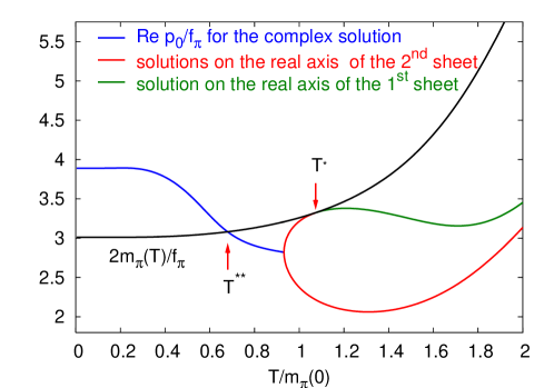
Figure 1: The temperature dependence if the real part of the sigma pole.

Following with the increasing temperature the trajectory of the complex sigma pole on the second Riemann sheet obtained in the O(N) model, with the help of the LO of the large N approximation, one can see that the real part of the sigma goes below the value of the two pion threshold at $T^{**}\approx 0.69m_{\pi}(0)=96.6$ MeV, which means the suppression of the $\sigma\to 2\pi$ decay channel [23]. This happens at a lower temperature than $T^{*}\approx 1.07m_{\pi}(0)$, where $\sigma$ is converted into a stable particle. So, for $T<T^{**}$ sigma is indeed a sharper resonance compared with the vacuum case. This scenario differs from the one in [24] where the pole that goes through the threshold is not connected with the complex sigma pole at $T=0$. By assuming certain analytic properties of the propagator, we have shown that there are universal features of the spectral function when a pole corresponding to a particle at high temperature approaches in the complex energy plane with the variation of the temperature the threshold position of its two-body decay [25].

It is interesting to note, that the value of the temperature where $m_{\sigma}=2m_{\pi}$ is quite close to what was found within the composite operator formalism applied to the QCD: $T^{**}=0.95T_{c}\simeq 98$ MeV [26]. Another interesting point is that within the large N formalism the mass of the sigma appears to be rather low (at NLO it is about 350 MeV, [27]).

The restoration of the chiral and axial symmetries was studied recently by many authors, using both the linear sigma model [28, 29],[14] and NJL [30]. The method of these studies was to identify the chiral partners and observe the convergence of their masses. The chiral partners are $(\pi,\sigma)$, $(\eta,a_{0})$ in the case of chiral SU(2) symmetry and $(\pi,a_{0})$, $(K,\kappa)$, $(\eta,\sigma)$ in the case of chiral SU(3) symmetry. The results of these investigations can be summarised as follows.

The scalar masses decrease at first but then start to increase during the transition while the pseudoscalar masses stay constant for a long while then increase monotonically with the temperature during the transition. The masses grow more rapidly when $N_{f}$ increases, and there is a tendency of the chiral partners towards degeneracy at some $T>T_{c}$. In the absence of $U_{A}(1)$ anomaly $T_{c}$ decreases, and the degeneracy is more rapidly reached. The melting of the strange condensate is much slower compared with the non-strange one.

For the effect of the $U(1)$ anomaly it was found that in the chiral limit with(out) $U_{A}(1)$ anomaly the transition temperature increases (decreases) with $N_{f}$ in contrast to (in agreement with) the QCD lattice results which according to [8] give for $N_{f}=2(3)$ $T_{c}\simeq 173(154)$ MeV. This signals that the anomaly is rapidly decreasing near the transition temperature. Indeed, this decrease can be observed, since the finite temperature lattice result on topological susceptibility [31] can be converted into the temperature-dependence of the strength of the determinant term, $g_{D}(T)$ by fitting the lattice result with the explicit formula of the susceptibility calculated in NJL [32]. In this case the determinant term decreases not only due to the very slow melting of the strange condensate, but also due to the decrease of $g_{D}(T)$. Hence $U_{A}(1)$ symmetry is restored and the degeneracy of the SU(3) chiral partners is completed. Without the restoration of the $U_{A}(1)$ symmetry the degeneracy among parity partners arises only at very high temperature at which the determinant term would eventually vanish due to the vanishing of the strange condensate. (We have to recall that the determinant enters with opposite sign into the expressions of the scalar and pseudoscalar masses.)

5 $\mu_{B}-T$ phase diagram for $N_{f}=2$

The left hand side figure of Fig. 2 shows a generic phase diagram typical for those obtained with effective models. In particular this figure was obtained for the chiral limit, solved in the LO of the large N approximation, with the fermions taken into account perturbatively at one loop order [21]. The emerging diagram is qualitatively correct, but when compared with lattice results, one observes that the transition temperature is too low (the lattice result of [33] is $T_{c}(\mu_{B}=0)=173(8)$MeV) and the present estimate for TCP is presumably located at a too high chemical potential.

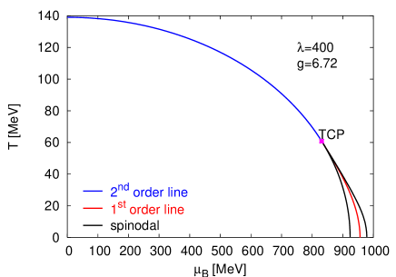
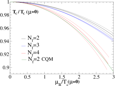
Figure 2: L.h.s.: The $\mu_{B}-T$ phase diagram of the constituent quark model in the chiral limit. R.h.s: Comparison of the CQM result from [21] with lattice results (from top to bottom): $N_{f}=2$ [34], $N_{f}=3$ [35], $N_{f}=4$ [36] (the original figure was taken from [35]).

The transition line, which is a parabola, and the location of TCP can be obtained analytically in terms of polylogarithms:

$$\left.\begin{array}[]{l}{2^{\textnormal{nd}}\,\textnormal{order+spinodal line}}\qquad\displaystyle m^{2}+\left(\frac{\lambda}{6}+g^{2}N_{c}\right)\frac{T^{2}_{c}}{12}+\frac{g^{2}\mu^{2}_{q}}{2\pi^{2}N_{f}}N_{c}=0,\vspace*{0.2cm}\\ {2^{\textnormal{nd}}\,\textnormal{order line ends when}}\qquad\displaystyle\frac{\lambda}{6}+\frac{g^{4}N_{c}}{4\pi^{2}}\left[\frac{\partial}{\partial n}\Big{(}\textrm{Li}_{n}\left(\frac{1}{z}\right)+\textrm{Li}_{n}\left(z\right)\Big{)}\Big{|}_{n=0}-\ln\frac{cT_{c}}{M_{0}}\right]=0\end{array}\right\}\Rightarrow\parbox[t]{34.14322pt}{$T_{TCP}$\\ $\mu_{TCP}.$}$$

These formulae are obtained by expanding the equation of state in a power series of the expectation value and by taking the coefficient of the linear and cubic terms, which correspond to the quadratic and quartic terms of the effective potential. In the formulae above $-z=e^{\frac{\mu_{q}}{T_{c}}}$ (the fugacity), $c=2e^{1-\gamma_{E}}$, $N_{c}=3$, and $M_{0}$ is the renormalisation scale.

The curvature of the line of second order phase transitions at $\mu_{q}=0$ is $\frac{T_{c}}{2}\frac{d^{2}T_{c}}{d\mu^{2}_{q}}\Big{|}_{\mu_{q}=0}=0.101$, which is somewhat higher than what is obtained on the lattice. (The masses are different, strictly speaking there is no much sense in comparing). This can be seen also in the r.h.s. of Fig. 2 taken from [35] in which we inserted our phase transition line (the green line which ends in the lower right corner of the figure). The reason for this is that the large value of the Yukawa coupling lowers the critical temperature at vanishing chemical potential and bends too strongly the transition line. We have checked that dynamical generation of the fermion mass, e.g. solving a gap equation for it, lowers the effective Yukawa coupling. This result and the fact that according to Fig. 2 the line of the reduced temperatures lies within 10% of the lattice result, mean that it might be worth thinking about a more complete inclusion of fermions, e.g. beyond one loop order.

By looking at different effective approaches published in the literature (see a list in [37]) we can see that all give low values for the temperature and high values for the chemical potential at TCP or CEP when compared with the result of Fodor and Katz [38]. This may be partly due to the fact that these results are for two flavors and not 2+1 ( it was emphasised in Ref. [39] how sensitive is the dependence of the critical value of $\mu_{B}$ on the value of the quark masses). But this also raises a conceptual problem of whether the QCD phase transition is driven by the chiral symmetry.

As was shown recently in [40] using renormalisation group techniques the inclusion of gluon degrees of freedom proves to be important at $T\approx 150$ MeV if one wants to compare the equation of state of the effective model with the one obtained on the lattice.

The conclusion of the resonance gas model (which includes 1026 resonances) is that the phase transition is driven by the higher excited hadrons rather than by the light degrees of freedom [41]. This model managed to reproduce the temperature dependence of the energy density measured on the lattice. It is interesting that a pion gas would give only 15% of the critical energy density at the transition temperature. Imposing constant energy density the resonance gas model also reproduced the phase boundary measured on the lattice using Taylor expansion in $\mu_{B}$.

The discrepancy between the freezout curve and phase boundary obtained with the resonance gas model shows that there are strong interactions between baryons and mesons when the density of the baryons exceeds the density of mesons and without interactions this model is not able to account for how criticality occurs.

I conclude that the investigation of the phase-diagram in the $\mu_{B}-T$ plane with an effective 3-flavor model is definitely of interest.

6 The nature of the soft mode

In the physical point of the quark mass-plane a critical end point was found on lattice [38] at a finite value of the chemical potential and the question is what causes criticality. At the critical end point two minima and a maximum meet which results in a very flat effective potential of the chiral order parameter $\Phi$. This is shown also by the diverging peak of the scalar susceptibility $d\Phi/dh$. This flattening of the effective potential does not necessarily imply the appearance of a gapless sigma mode (sigma meson with vanishing mass). This is because the non-interchangeability of two limits : ${\bf q}$-limit ($\omega\to 0$, then ${\bf q}\to{\bf 0}$), which applies to static quantities as the curvature of the effective potential, and $\omega$-limit (${\bf q}\to{\bf 0}$, then $\omega\to 0$), which applies to the study of a sigma pole at rest on the second Riemann sheet (resonance).

It was argued in Ref. [42] that what is important from the point of view of the signature of the genuinely singular end point is the dynamical feature rather than the static one. The time during which the correlation length $\xi$ reaches its equilibrium diverges as $\tau\sim\xi^{z}$ (critical slowing down), where $z$ is the dynamic scaling exponent. The finite evolution time limits the correlation length to $\xi<(\rm{time})^{1/z}$. Because $z>1$ and in heavy-ion collision the evolution times are of the same order as the spatial size, it is the finite time of the evolution rather than the spatial size limitation ($\xi<$size), which imposes a limit on the value of $\xi$. This is why, it is important to find the dynamical universality class CEP belongs to, according to the classification of [43], and also the correct identification of the soft mode, the mode whose characteristic frequency vanishes at CEP, and which determines the characteristic time of the evolution.

I refer the reader to the literature in questions which concern the hydrodynamical nature of the soft mode, in presence of conserved baryon number and energy densities, and on the demonstration that the dynamic universality class of CEP is that of model H, i.e. the liquid-gas phase transition [43], [42], [44]. Here I will discuss what can be found about the nature of the soft mode with model calculations focusing on the scalar order parameter.

In the O(4) model without explicit symmetry breaking there is a genuine second order transition accompanied by a change in the symmetry of the ground state. Here, what is responsible for the critical behaviour and dynamical scaling is the pole in the sigma channel [45]. Following the trajectory of the sigma pole (corresponding to the particle a rest) of the analytically continued Green’s function on the second Riemann sheet, it turns out that the pole arrives on the imaginary axis, splits up into two poles, and the one that goes to the origin will produce critical scaling. In the vicinity of the critical point the dynamical scaling and the equation for the soft mode were given in [45] (see also the references therein).

In the 2 flavor constituent quark model in the chiral limit, along the line of the chiral critical points, the soft mode is also the sigma meson, which becomes the degenerate chiral partner of the massless pions. The sigma pole on the 2nd Riemann sheet goes to the origin as the order parameter $\Phi(T)$ goes to zero. The real and imaginary parts of the pole scale as $\textnormal{Re}p_{0}\sim\Phi(T)$, $\textnormal{Im}p_{0}\sim\Phi^{2}(T)$, where $\Phi\sim(T-T_{c})^{\beta}$. For $\beta$ the mean-field exponent was obtained [21] : $\beta=1/2$ for the second order line and $\beta=1/4$ at the tricritical point. The case of TCP is interesting because it prompts the question of what kind of singular behaviour might appear additionally there, where the sigma meson mode is already gapless (see below).

For the physical pion mass and two flavors no symmetry change of the ground state accompanies the second order transition at CEP and in consequence from the point of view of the symmetry the existence of CEP is accidental. Both in CQM [46] and NJL [47] the sigma pole stays massive, and a peak develops in the scalar isoscalar spectral function in the space-like region $\omega<|{\bf q}|$. The location of its maximum goes to zero as the momentum goes to zero and it diverges in the ${\bf q}$-limit.

In the context of the NJL model what is responsible for the behaviour seen in the spectral functions is an imaginary pole of the scalar susceptibility ($\chi_{mm}=d^{2}F(T,\mu)/dm^{2}_{ud}=d\langle\bar{q}q\rangle/dm_{ud}$, where $F(T,\mu)$ is the free energy density) that goes to the origin as $|{\bf q}|\to 0$ (diffusive mode) [47]. In consequence the soft mode is the fluctuation of the scalar density. To study the relative weight of the diffusive mode in the susceptibility, the ratio $R=(\chi_{mm}(0,{\bf 0}^{+})-\chi_{mm}(0^{+},{\bf 0}))/\chi_{mm}(0,{\bf 0}^{+})$ was introduced, where the numerator is the difference between the ${\bf q}$-limit and $\omega$-limit. When the diffusive mode is absent $R=0$. Because there is no contribution from the diffusive mode in the second term of the numerator, when the diffusive mode dominates $R\to 1$. By studying this ratio $R$, it was shown in [44] that the switch of the soft mode from the sigma meson mode to the diffusive mode (hydrodynamical mode) occurs at the tricritical point, where $R=1$.

7 The boundary of the first order phase transition in the $m_{\pi}-m_{K}$–plane

There are several lattice studies of thermodynamics with varying degenerate quarks $m_{u}=m_{d}=m_{s}$, which show that the value of $m_{PS}^{c}$ on the boundary drops substantially when improved lattice actions are used, namely from $m_{\pi}^{c}\approx 290$ MeV [48] or $m_{\pi}^{c}\approx 270$ MeV [49] to $m_{\pi}^{c}=67(18)$ MeV [50] or ever further down to $m_{\pi}^{c}<65$ MeV [51] (see also the talk by O. Philipsen at this meeting). In view of this result we can think that the linear sigma model might complement lattice investigations if its coupling parameters can be determined accurately because the lighter are the pseudoscalars the better should become the approximate description based on L$\sigma$M. This model was claimed to give a low value for the critical pion mass: $m_{\pi}^{c}=51$ MeV [52] or $m_{\pi}^{c}=47$ MeV [53] (see also [29]). In these investigations only the Goldstone mass was tuned by varying the explicit symmetry breaking terms and the other parameters were kept fixed at their values determined in the physical point.

We have used ChPT when moving away from the physical point [18] for the determination of the pion and kaon decay constants and $M_{\eta}^{2}=m_{\eta}^{2}+m^{2}_{\eta^{\prime}}$, to obtain the value of the couplings at each point of the $m_{\pi}-m_{K}$–plane (see Eqs. (4), (5), and (6)). Below I present schematically how the process of the parametrisation is performed.

input:

output:

prediction:

$$\left.\begin{aligned} \left.\begin{aligned} f_{\pi}\,\,\\ f_{K}\,\,\end{aligned}\right\}&\Longrightarrow&\begin{aligned} x\quad\,\\ y\quad\,\end{aligned}\\ \left.\begin{aligned} m_{\pi}\,\\ m_{K}\,\\ M_{\eta}^{2}\end{aligned}\right\}&\Longrightarrow&\begin{aligned} g\quad\,\\ f_{2}\quad\\ M^{2}\,\,\,\end{aligned}\end{aligned}\right\}\Longrightarrow\begin{aligned} m_{\eta}\,\,\,\,\,\,\,\quad\quad\quad\\ m_{\eta^{\prime}}\,\,\,\,\quad\quad\quad\\ \theta_{\eta}\quad\quad\quad\quad\\ m_{a_{0}}\,\,\,\quad\quad\quad\\ m_{\kappa}\,\,\,\,\quad\quad\quad\end{aligned}$$

$$\begin{aligned} \left.\begin{aligned} \textnormal{A1 \& ${M}^{2}$}\,\\ \textnormal{A2 \& ${M}^{2}$}\,\end{aligned}\right\}&\Longrightarrow&\left.\begin{aligned} \mu_{0}^{2}\,\,\,\,\,\\ f_{1}\,\,\,\,\,\end{aligned}\right\}\Longrightarrow\begin{aligned} m_{\sigma}\\ m_{f_{0}}\\ \theta_{\sigma}\end{aligned}\,\,\qquad\quad\\ \left.\begin{aligned} E_{x}=0\,\,\,\\ E_{y}=0\,\,\,\end{aligned}\right\}&\Longrightarrow&\begin{aligned} h_{x}\quad\quad\quad\quad\quad\quad\,\,\,\quad\quad\quad\\ h_{y}\quad\quad\quad\quad\quad\quad\,\,\,\quad\quad\quad\end{aligned}\end{aligned}$$

The strange and non-strange condensates are determined through the PCAC relations $x=f_{\pi}$, $y=(2f_{K}-f_{\pi})/\sqrt{2}$, while the masses determine the couplings (for the explicit formulae see [28] or [18]). The predicted values of $m_{\eta}$ and $m_{\eta}^{\prime}$ are in remarkable agreement with the values of these masses given by ChPT up to $m_{K}=800$ MeV, even for vanishing pion mass. Unfortunately, at tree-level, in the pseudoscalar sector one of the quartic couplings, $f_{1}$ and the mass parameter $\mu_{0}^{2}$ appear only in the combination $M^{2}=-\mu_{0}^{2}+4f_{1}(x^{2}+y^{2})$. To disentangle them we have to use also the scalar sector. Since the dependence of scalar masses on $m_{\pi}$ and $m_{K}$ is not known, we need to make assumptions, which diminish the predictive power of our solution. This can be seen in Fig. 3 which shows the boundary of the first order transition region on the $(m_{\pi}-m_{K})$-plane for various assumptions made for the continuation of the scalar mass spectrum. We expect that the exact phase boundary curve lies in the light-grey shaded region.

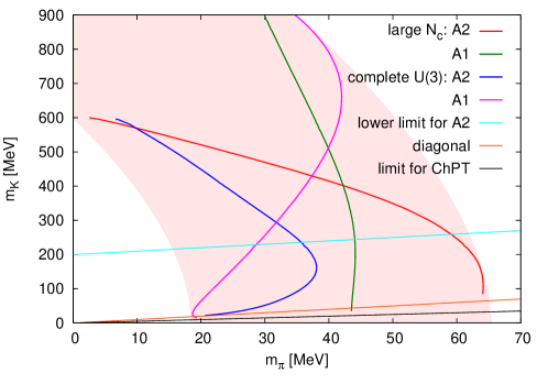
Figure 3: Phase boundary for different alternatives. A1: it is assumed that there is no mixing in the scalar $x-y$ sector ($m^{2}_{\sigma_{xy}}=0$) A2: it is assumed that the $SU_{L}(3)\times SU_{R}(3)$ Gell-Mann–Okubo mass formula for the scalars is satisfied in the full $(m_{\pi}-m_{K})$-plane with the same accuracy as at the physical point. We consider complete U(3) ChPT and the leading order large-$N_{c}$ ChPT at $\mathcal{O}(p^{2})$. Crossover (first order transition) takes places at the right (left) of the shaded region.

Our rough estimate for the critical pion mass on the diagonal is $m_{\textrm{crit}}(\textrm{diag})=40\pm 20$ MeV, in nice agreement with the results of the latest effective model and lattice studies. In order to be able to use the tree-level parametrisation we used a quasi-particle approximation, that is we neglected the finite parts of the $T=0$ quantum fluctuations. We note, that we were not able to locate the TCP on the $m_{u,d}=0$ axis. Recently a work performed in the NJL model found the TCP at the critical value of $m_{s}^{c}=10$ MeV [54], which is much lower than expected when extrapolating lattice results.

8 Conclusions

In this contribution we reviewed some of the results obtained with effective models of QCD on the chiral symmetry restoration. We have shown that one can parameterise the linear sigma model in the entire $m_{\pi}-m_{K}$–plane employing the results of the chiral perturbation theory. We have determined the boundary of the first order phase transition line which is below $m_{\pi}^{c}=65$ MeV. For a more reliable determination of the boundary, information on the quark-mass dependence of the scalar sector is needed.

We have shown that effective models correctly describe the changes of the meson properties during the chiral transition and indicate that $U_{A}(1)$ has to be restored as a prerequisite for restoration of $SU(3)$ chiral symmetry. The sigma meson is the soft mode at the critical point of the O(4) model with massless pions, and in both the 2 flavor constituent quark model and NJL model in the chiral limit along the line of the chiral critical points, but stays massive at CEP. At CEP the role of the chiral symmetry is rather secondary, here the soft mode has a hydrodynamical nature.

An analytical determination of the $\mu-T$ phase boundary was given for two flavors in the chiral limit. The obtained phase diagram is qualitatively correct, but the transition temperature is low and the value of the chemical potential at TCP/CEP is apparently too high. Light mesonic degrees of freedom, usually included into effective theories of QCD do not seem to be the single driving force behind the transition. In view of this, the extension of the 3-flavor chiral quark model to finite density is of imminent importance. It would be also interesting to develop large N techniques for $SU_{L}(N)\times SU_{R}(N)$ chiral models, since this approach has some advantage when used together with other resummation techniques (2PI or Dyson-Schwinger).

- [1] A. Ukawa, Lectures on Lattice QCD at finite temperature, in Uehling Summer School “Phenomenology and Lattice QCD” (1993), [available on-line on SPIRES-HEP].
- [2] M. Stephanov, K. Rajagopal, E. Shuryak Phys. Rev. D 60, 114028 (1999) [hep-ph/9903292].
- [3] B. Berdnikov and K. Rajagopal, Phys. Rev. D 61, 105017 (2000) [hep-ph/9912274].
- [4] Sz. Borsanyi, A. Patkos, D. Sexty, Zs. Szep, Phys. Rev. D 64, 125011 (2001) [hep-ph/0105332].
- [5] M. Hindmarsh and O. Philipsen, Phys. Rev. D 71, 087302 (2005) [hep-ph/0501232]; see also the talk of M. Hindmarsh at the present meeting.
- [6] A. Mocsy, F. Sannino, K. Tuominen, J. Phys. G30, S1255-S1258 (2004) [hep-ph/0403160].
- [7] K. Fukushima, Phys. Lett. B591, 277-284 (2004) [hep-ph/0310121].
- [8] F. Karsch, Lect. Notes Phys. 583, 209 (2002) [hep-lat/0106019].
- [9] J. Gasser and H. Leutwyler, Nucl. Phys. B250, 465 (1985).
- [10] N. Beisert and B. Borasoy, Eur. Phys. J. A 11, 329 (2001) [hep-ph/0107175].
- [11] Y. Nambu and G. Jona-Lasinio, Phys. Rev. 122, 345 (1961).
- [12] M.K. Volkov, A.E. Radzhabov, Forty-fifth anniversary of the Nambu-Jona-Lasinio model, [hep-ph/0508263].
- [13] S. Gasiorowicz and D. A. Geffen, Rev. Mod. Phys. 41, 531 (1969); L.-H. Chan and R. W. Haymaker, Phys. Rev. D 7, 402 (1973).
- [14] D. Röder, J. Ruppert, D. H. Rischke, Phys. Rev. D 68, 016003 (2003) [nucl-th/0301085] .
- [15] F. Wilczek, Int. J. Mod. Phys. D3, Suppl., 63-80 (1994) [available on-line on SPIRES-HEP].
- [16] S. Chiku, T. Hatsuda, Phys. Rev. D 58, 076001 (1998) [hep-ph/9803226].
- [17] A. Jakovác, Zs. Szép, Phys. Rev. D 71, 105001 (2005) [hep-ph/0405226].
- [18] T. Herpay, A. Patkós, Zs. Szép and P. Szépfalusy, Phys. Rev. D 71, 125017 (2005) [hep-ph/0504167].
- [19] J. M. Cornwall, R. Jackiw, and E. Tomboulis, Phys. Rev. D 10, 2428 (1974).
- [20] N. Petropoulos, J. Phys. G25, 2225 (1999) [hep-ph/9807331].
- [21] A. Jakovác, A. Patkós, Zs. Szép, P. Szépfalusy, Phys. Lett. B582, 179 (2004) [hep-ph/0312088].
- [22] T. Hatsuda, T. Kunihiro, Phys. Rev. Lett. 55, 158 (1985).
- [23] A. Patkós, Zs. Szép, P. Szépfalusy Phys. Rev. D 66, 116004 (2002). [hep-ph/0206040]
- [24] Y. Hidaka, O. Morimatsu, T. Nishikawa, Phys. Rev. D 67, 056004 (2003) [hep-ph/0211015].
- [25] A. Patkós, Zs. Szép, P. Szépfalusy, Phys. Rev. D 68, 047701 (2003) [hep-ph/0305100].
- [26] A. Barducci, R. Casalbuoni, R. Gatto, M. Modugno, G. Pettini, Phys. Rev. D 59, 114024 (1999) [hep-ph/9810245].
- [27] J. O. Andersen, D. Boer, H. J. Warringa, Phys. Rev. D 70, 116 (2004) [hep-ph/0408033].
- [28] J. T. Lenaghan, D. H. Rischke, J. Schaffner-Bielich, Phys. Rev. D 62, 085008 (2000) [nucl-th/0004006].
- [29] J. T. Lenaghan, Phys. Rev. D 63, 037901 (2001) [hep-ph/0005330].
- [30] P. Costa, M. C. Ruivo, C. A de Sousa and Yu. L. Kalinovsky, Phys. Rev. D 71, 116002 (2005) [hep-ph/0503258].
- [31] B. Allés, M. D’Elia, A. Di Giacomo, Nucl. Phys. B494, 281 (1997) [hep-lat/9605013] , Erratum-ibid. B679 (2004) 397-399.
- [32] K. Ohnishi, K. Fukushima, K. Ohta, Phys.Rev. C 63, 045203 (2001) [nucl-th/0101062].
- [33] F. Karsch, E. Laermann, A. Peikert, Nucl. Phys B605, 579 (2001) [hep-lat/0012023].
- [34] Ph. de Forcrand, O. Philipsen, Nucl. Phys. B642, 290 (2002) [hep-lat/0205016].
- [35] Ph. de Forcrand, O. Philipsen, Nucl. Phys. B673, 170 (2003) [hep-lat/0307020].
- [36] M. D’Elia, M.-P. Lombardo, Phys. Rev. D 67, 014505 (2003) [hep-lat/0209146].
- [37] M. Stephanov, Progress of Theoretical Physics Supplement 153, 139 (2004) [hep-ph/0402115].
- [38] Z. Fodor, S. D. Katz, JHEP 0404, 050 (2004) [hep-lat/0402006].
- [39] O. Philipsen, The QCD phase diagram at zero and small baryon density, in proc. of LATTICE 2005: XXIII International Symposium on Lattice Field Theory, PoS(LAT2005) 016, [hep-lat/0510077].
- [40] J. Braun, K. Schwenzer, H.-J. Pirner, Phys. Rev. D 70, 085016 (2004) [hep-ph/0312277].
- [41] F. Karsch, K. Redlich, A. Tawfik, Eur. Phys. J. C 29, 549 (2003) [hep-ph/0303108].
- [42] D. T. Son and M. A. Stephanov, Phys. Rev. D 70, 056001 (2004) [hep-ph/0401052].
- [43] P. C. Hohenberg and B. I. Halperin, Rev. Mod. Phys. 49, 435 (1977).
- [44] H. Fujii and M. Ohtani, Phys. Rev. D 70, 014016 (2004) [hep-ph/0402263].
- [45] A. Patkós, Zs. Szép, P. Szépfalusy, Phys. Lett. B537, 77 (2002) [hep-ph/0202261].
- [46] A. Jakovác, A. Patkós, Zs. Szép, P. Szépfalusy, in Proc. of SEWM 2004, Helsinki, Eds. K. J. Eskola et al., p. 196 [hep-ph/0409076].
- [47] H. Fujii, Phys. Rev. D 67, 094018 (2003) [hep-ph/0302167].
- [48] F. Karsch, E. Laermann, Ch. Schmidt, Phys. Lett. B520, 41 (2001) [hep-lat/0107020].
- [49] N. H. Christ, X. Liao, Nucl. Phys. Proc. Suppl. 119, 514 (2003).
- [50] F. Karsch, C. R. Allton, S. Ejiri, S. J. Hands, O. Kaczmarek, E. Laermann and C. Schmidt, Nucl. Phys. Proc. Suppl. 129-130, 614 (2004) [hep-lat/0309116].
- [51] The MILC Collaboration: C. Bernard, T. Burch, C. DeTar, S. Gottlieb, E.B. Gregory, U.M. Heller, J. Osborn, R.L. Sugar, D. Toussaint [hep-lat/0409097].
- [52] H. Meyer-Ortmanns and B. Schæfer, Phys. Rev. D 53, 6586 (1996) [hep-ph/9409430] .
- [53] C. Schmidt, PhD Thesis, Bielefeld University, 2003; result quoted in [50], [available online at ftp://ftp.uni-bielefeld.de/pub/papers/physik/theory/e6/dissertationen/schmidt.ps.gz].
- [54] A. Barducci, R. Casalbuoni, G. Pettini, L. Ravagli, Phys. Rev. D 72, 056002 (2005) [hep-ph/0508117].