DESY 05-238

Squarks and Sleptons between Branes and Bulk

Wilfried Buchmüller, Jörn Kersten and Kai Schmidt-Hoberg

Deutsches Elektronen-Synchrotron DESY, 22603 Hamburg, Germany

We study gaugino-mediated supersymmetry breaking in a six-dimensional $SO(10)$ orbifold GUT model where quarks and leptons are mixtures of brane and bulk fields. The couplings of bulk matter fields to the supersymmetry breaking brane field have to be suppressed in order to avoid large FCNCs. We derive bounds on the soft supersymmetry breaking parameters and calculate the superparticle mass spectrum. If the gravitino is the LSP, the $\tilde{\tau}_{1}$ or the $\tilde{\nu}_{\tau\mathrm{L}}$ turns out to be the NLSP, with characteristic signatures at future colliders and in cosmology.

1 Introduction

With the start of the LHC and the possible observation of superparticles approaching, there is an increasing interest in specific predictions for their mass spectrum, which results from the interplay between fermion mass models and models for supersymmetry breaking. Supersymmetric orbifold GUTs [1] are attractive candidates for unified theories explaining the masses and mixings of fermions. Features such as the doublet-triplet splitting and the absence of dimension-five operators for proton decay, which are difficult to realise in four-dimensional grand unified theories, are easily obtained. Given the higher-dimensional setup with various branes, the mechanism of supersymmetry breaking involves in general bulk as well as brane fields.

Following this rationale, we consider an $SO(10)$ theory in six dimensions, proposed in [8], in combination with gaugino-mediated SUSY breaking [9, 10]. The orbifold compactification of the two extra dimensions has four fixed points or “branes”. On three of them, three quark-lepton generations are localised. The Standard Model leptons and down-type quarks are linear combinations of these localised fermions and a partial fourth generation living in the bulk. This leads to the observed large neutrino mixings. On the fourth brane, we assume a gauge-singlet field $S$ to develop an $F$-term vacuum expectation value (vev) breaking SUSY. As the gauge and Higgs fields propagate in the bulk, they feel the effects of SUSY breaking. Thus, gauginos and Higgs scalars obtain soft masses. The soft masses and trilinear couplings of the scalar quarks and leptons approximately vanish at the compactification scale. Non-zero values are generated by the running to low energies, which leads to a realistic superparticle mass spectrum. If the gravitino is the lightest superparticle (LSP), it can be the dominant component of the dark matter. The next-to-lightest superparticle (NLSP) is then a scalar tau or a scalar neutrino, which is consistent with constraints from big bang nucleosynthesis.

In the next section, we will describe the orbifold model and the couplings needed for SUSY breaking. Subsequently, we will demonstrate that the presence of extra matter fields in the bulk leads to severe problems with flavour-changing neutral currents (FCNCs) unless the couplings of these fields to the SUSY-breaking field $S$ are suppressed. Using naïve dimensional analysis (NDA), we derive upper bounds on the unknown couplings of the theory and thus on the non-vanishing soft masses, $\mu$ and $B\mu$ at high energy. Finally, we calculate the low-energy superparticle mass spectrum. A realistic spectrum requires the soft Higgs masses to satisfy bounds which are slightly stronger than those estimated by NDA.

2 The Orbifold GUT Model

We consider an $N=1$ supersymmetric $SO(10)$ gauge theory in six dimensions compactified on the orbifold $T^{2}/\left({\mathbbm{Z}}_{2}\times{\mathbbm{Z}}_{2}^{\prime}\times{\mathbbm{Z}}_{2}^{\prime\prime}\right)$ [8]. The theory has four fixed points, $O_{\text{\sc i}}$, $O_{\text{\sc ps}}$, $O_{\text{\sc gg}}$ and $O_{\text{fl}}$, located at the corners of a “pillow” corresponding to the two compact dimensions. At $O_{\text{\sc i}}$ the full $SO(10)$ survives, whereas at the other fixed points, $O_{\text{\sc ps}}$, $O_{\text{\sc gg}}$ and $O_{\text{fl}}$, $SO(10)$ is broken to its three GUT subgroups ${G}_{\text{\sc ps}}={SU(4)}\times{SU(2)}\times{SU(2)}$, ${G}_{\text{\sc gg}}={SU(5)}\times{U(1)}_{X}$ and flipped $SU(5)$, ${G}_{\text{fl}}={SU(5)^{\prime}}\times{U(1)^{\prime}}$, respectively. The intersection of these GUT groups yields the Standard Model group with an additional $U(1)$ factor, ${G}_{\text{\sc sm}^{\prime}}={SU(3)}\times{SU(2)}\times{U(1)}_{Y}\times{U(1)}_{X}$, as unbroken gauge symmetry below the compactification scale, which we identify with the GUT scale.

The field content of the theory is strongly constrained by requiring the cancellation of bulk and brane anomalies. The brane fields are the three 16-plets $\psi_{i}$, $i=1,2,3$. The bulk contains six 10-plets, $H_{1},\dots,H_{6}$, and four 16-plets, $\Phi,\Phi^{c},\phi,\phi^{c}$, as hypermultiplets. Vevs of $\Phi$ and $\Phi^{c}$ break the surviving ${U(1)}_{B-L}$. The electroweak gauge group is broken by expectation values of the doublets contained in $H_{1}$ and $H_{2}$.

We choose the parities of $\phi,\phi^{c}$ and $H_{5},H_{6}$ such that their zero modes are

$$L=\left(\begin{array}[]{l}\nu_{4}\\ e_{4}\end{array}\right)\;,\quad L^{c}=\left(\begin{array}[]{l}n^{c}_{4}\\ e^{c}_{4}\end{array}\right)\;,\quad G^{c}_{5}=d^{c}_{4}\;,\quad G_{6}=d_{4}\;.$$ (5)

These zero modes act as a fourth generation of down (s)quarks and (s)leptons and mix with the three generations of brane fields. We allocate the three sequential 16-plets to the three branes where $SO(10)$ is broken to its three GUT subgroups, placing $\psi_{1}$ at $O_{\text{\sc gg}}$, $\psi_{2}$ at $O_{\text{fl}}$ and $\psi_{3}$ at $O_{\text{\sc ps}}$. The three “families” are then separated by distances large compared to the cutoff scale $\Lambda$. Hence, they can only have diagonal Yukawa couplings with the bulk Higgs fields. The brane fields, however, can mix with the bulk zero modes without suppression. As these mixings take place only among left-handed leptons and right-handed down-quarks, we obtain a characteristic pattern of mass matrices.

The model has the minimal amount of supersymmetry in six dimensions, corresponding to $N=2$ extended supersymmetry in four dimensions. The breaking to $N=1$ supersymmetry at the four-dimensional fixed points is achieved by the ${\mathbbm{Z}}_{2}$-symmetry. Soft SUSY-breaking terms are generated by gaugino mediation [9, 10]. We place the gauge-singlet chiral superfield $S$, which acquires a non-vanishing vev for its $F$-term component, at the fixed point $O_{\text{\sc i}}$. Supersymmetry is then fully broken and the breaking can be communicated to gauge, Higgs and other bulk fields by direct interactions. The MSSM squarks and sleptons that live on branes can obtain soft SUSY-breaking masses via loop contributions through the bulk, which are negligible here, and via renormalisation group running. To study the scalar masses and mixings we first have to discuss all couplings which can lead to mass terms.

2.1 The Superpotential

The superpotential determines the SUSY-conserving mass terms and Yukawa couplings. The allowed terms are restricted by $R$-invariance and an additional $U(1)_{\tilde{X}}$ symmetry with the charge assignments given in Tab. 1. Starting from the six-dimensional theory, the effective four-dimensional fields are obtained by integrating out the two extra dimensions. This leads to a volume factor between the original six-dimensional fields and the properly normalised fields we use here, $\Phi=\sqrt{V}\Phi_{6}$.

The most general brane superpotential without the singlet field $S$ is given in [8]. All zero modes which have not been given in Eq. (5) can be found in [11]. Since the fields $\psi_{i}$ and $\phi$ have the same quantum numbers, they are combined to the quartet $\psi_{\alpha}=(\psi_{i},\phi)$. When the bulk fields are replaced by their zero modes, only $9$ of the $23$ terms appearing in the superpotential remain. They are given by

$$W= \;M^{d}H_{5}H_{6}+M^{l}_{\alpha}\psi_{\alpha}\phi^{c}+\frac{1}{2}h^{(1)}_{\alpha\beta}\psi_{\alpha}\psi_{\beta}H_{1}+\frac{1}{2}h^{(2)}_{\alpha\beta}\psi_{\alpha}\psi_{\beta}H_{2}+f_{\alpha}\Phi\psi_{\alpha}H_{6}$$

$${}+\frac{h^{N}_{\alpha\beta}}{2\Lambda}\psi_{\alpha}\psi_{\beta}\Phi^{c}\Phi^{c}+\frac{g_{\alpha}^{d}}{\Lambda}\Phi^{c}\psi_{\alpha}H_{5}H_{1}+f^{D}\Phi^{c}\Phi^{c}H_{3}+f^{G}\Phi\Phi H_{4}\;.$$ (6)

	$H_{1}$	$H_{2}$	$\Phi^{c}$	$H_{3}$	$\Phi$	$H_{4}$	$\psi_{i}$	$\phi^{c}$	$\phi$	$H_{5}$	$H_{6}$	$S$
$R$	0	0	0	2	0	2	1	1	1	1	1	0
$\tilde{X}$	-2a	-2a	-a	2a	a	-2a	a	-a	a	2a	-2a	0

Table 1: Charge assignments for the symmetries $U(1)_{R}$ and $U(1)_{\tilde{X}}$

Consider now terms which involve the supersymmetry breaking singlet field $S$. We want the brane Lagrangian to yield gaugino masses, since they cannot be generated radiatively when starting from a vanishing mass at the compactification scale. Therefore, the source brane Lagrangian coupling the zero modes of the gauge fields to the chiral field on the source brane takes the form

$$\mathscr{L}_{S}\supset\frac{g_{4}^{2}h}{4\Lambda}\,\int\text{d}^{2}\theta\,S\,W^{\alpha}W_{\alpha}+\text{h.c.}\;,$$ (7)

where $g_{4}$ is the four-dimensional gauge coupling and $h$ is a dimensionless coupling. From this equation and the ordinary kinetic term $\frac{1}{4}\int\text{d}^{2}\theta\,W^{\alpha}W_{\alpha}+\text{h.c.}$ for the gauge fields we conclude that $S$ must have $U(1)_{\tilde{X}}$- and $R$-charge $0$ to leave the Lagrangian invariant. Therefore, terms respecting all the symmetries including $U(1)_{\tilde{X}}$ are simply given by

$$\mathscr{L}_{S}\propto\int\text{d}^{2}\theta\,\frac{S}{\Lambda}\,W+\text{h.c.}\;,$$ (8)

where $W$ is the superpotential given above and where we only keep those terms of $W$ which are at most cubic in the fields. Note that in addition $\psi_{\alpha}$ has to be replaced by $\phi$, since the matter fields $\psi_{i}$ cannot have direct couplings to the source brane. Moreover, we are interested only in terms which are non-zero when replacing the fields by their zero modes. A 16-plet $\psi$ of $SO(10)$ is written in standard notation as $\psi=(q,u^{c},e^{c},l,d^{c},n^{c}).$ When setting the chiral field $S$ to its vev $F_{S}$, the scalar components of the superfields remain, whereas the fermionic components are projected out. When furthermore the 16-plets $\Phi,\Phi^{c}$ acquire a vev $\langle\Phi\rangle=\langle\Phi^{c}\rangle=v_{N}\sim M_{\mathrm{GUT}}$ leading to the spontaneous breakdown of $U(1)_{B-L}$ we obtain (cf. Eq. (5))

$$\mathscr{L}_{S}\supset-\int\text{d}^{2}\theta\;\frac{S}{\Lambda}\left(\tilde{M}^{d}\tilde{d}_{4}^{c}\tilde{d}_{4}+\tilde{M}^{l}_{4}\tilde{l}_{4}\tilde{l}_{4}^{c}\right)+\text{h.c.}\,.$$ (9)

Additional terms involving the heavy fields $\Phi,\Phi^{c}$ have been dropped. Note that $U(1)_{B-L}$ is a subgroup of the local symmetry $U(1)_{Y}\times U(1)_{X}$. The vevs $\langle\Phi\rangle=\langle\Phi^{c}\rangle$ break $U(1)_{X}\times U(1)_{\tilde{X}}$ to a $U(1)$ subgroup. As discussed in [11], the superpotential (2.1) then yields masses of order $M_{\mathrm{GUT}}$ for unwanted colour triplets contained in $\Phi,\Phi^{c},H_{3}$ and $H_{4}$. In this way, the unification of gauge couplings is maintained.

2.2 The Kähler Potential

In addition, soft mass terms can arise from the Kähler potential. We assume the global $U(1)_{\tilde{X}}$ symmetry to be only approximate and allow for explicit breaking here. This is necessary in order to obtain a $\mu$-term, which is not allowed in the superpotential, since the combination $H_{1}H_{2}$ is not invariant under $U(1)_{\tilde{X}}$. Besides, an explicit breaking of $U(1)_{\tilde{X}}$ is in fact required in order to avoid Goldstone bosons. Terms which result in non-negligible effects have to involve fields which acquire a large vev in order to compensate for the suppression by the cutoff scale $\Lambda$. In our case, large vevs are acquired by $\Phi$, $\Phi^{c}$ and $S$. We find that all terms without the singlet field $S$ do not contribute to any soft masses but merely give corrections to the kinetic terms. Concentrating on the terms involving $S$, we do not consider terms with heavy fields that have no influence on low-energy physics. In terms of the zero modes, the relevant part of the Kähler potential is

$$\mathscr{L}_{S}\supset -\int\text{d}^{4}\theta\,\bigg{\{}\frac{S^{\dagger}}{\Lambda}\left(aH_{2}H_{1}^{c}+b_{1}H_{1}^{c\dagger}H_{1}^{c}+b_{2}H_{2}^{\dagger}H_{2}\right)+\text{h.c.}$$

$$\hskip 56.9055pt+\frac{1}{\Lambda^{2}}S^{\dagger}S\left[c_{1}H_{1}^{c\dagger}H_{1}^{c}+c_{2}H_{2}^{\dagger}H_{2}+\left(dH_{2}H_{1}^{c}+\text{h.c.}\right)\right]\bigg{\}}$$

$${}-\int\text{d}^{4}\theta\,\bigg{\{}\frac{e_{i}}{\Lambda}S^{\dagger}B_{i}^{\dagger}B_{i}+\text{h.c.}+\frac{e_{i}^{\prime}}{\Lambda^{2}}S^{\dagger}S\,B_{i}^{\dagger}B_{i}\bigg{\}}\;,$$ (10)

yielding an effective $\mu$-term, soft Higgs masses, a $B\mu$-term and soft masses for all other bulk fields. $B_{i}$ ($i=1,\dots$) stands for any bulk matter field except $H_{1,2}$. Although the $\mu$-term itself is not a soft term, it is generated only after the breaking of supersymmetry via the Giudice-Masiero mechanism [12]. Note that there would be no electroweak symmetry breaking without the breaking of SUSY and hence no massive (s)particles at the electroweak scale.

To see the contributions to the soft masses explicitly, we express the Lagrangian by component fields, plugging in the $F$-term vev $F_{S}$ and the scalar vev $v_{N}$. Furthermore, we employ the equations of motion for the auxiliary fields and assume real couplings for simplicity. Concentrating on the fourth generation and on the Higgs fields, this results in the following scalar mass terms:

$$\mathscr{L}_{S}\supset -\frac{F_{S}^{\dagger}F_{S}}{\Lambda^{2}}\Big{[}\left(a^{2}+b_{1}^{2}+c_{1}\right)\tilde{h}_{1}^{c\dagger}\tilde{h}_{1}^{c}+\left(a^{2}+b_{2}^{2}+c_{2}\right)\tilde{h}_{2}^{\dagger}\tilde{h}_{2}$$

$$\hskip 51.21495pt+\left(\vphantom{a_{1}^{2}}a\,(b_{1}+b_{2})+d\right)\tilde{h}_{1}^{c}\tilde{h}_{2}+\text{h.c.}\Big{]}$$

$$-\frac{F_{S}^{\dagger}F_{S}}{\Lambda^{2}}\Big{[}\left(e_{d}^{2}+e_{d}^{\prime}\right)\tilde{d}_{4}^{\dagger}\tilde{d}_{4}+\left(e_{d^{c}}^{2}+e_{d^{c}}^{\prime}\right)\tilde{d}_{4}^{c\dagger}\tilde{d}_{4}^{c}+\left(e_{l}^{2}+e_{l}^{\prime}\right)\tilde{l}_{4}^{\dagger}\tilde{l}_{4}+\left(e_{l^{c}}^{2}+e_{l^{c}}^{\prime}\right)\tilde{l}_{4}^{c\dagger}\tilde{l}_{4}^{c}\Big{]}$$

$$-\frac{F_{S}}{\Lambda}\Big{[}\tilde{M}^{d}\tilde{d}_{4}^{c}\tilde{d}_{4}+\tilde{M}^{l}_{4}\tilde{l}_{4}\tilde{l}_{4}^{c}\Big{]}+\text{h.c.}\;,$$ (11)

where we have included the contribution from Eq. (9) in the last line. We denote the components of a chiral multiplet by $(\tilde{\phi},\phi,F_{\Phi})$, with $\Phi=H_{1}^{c},H_{2},d_{4},d_{4}^{c},l_{4},l_{4}^{c}$. Note that the Higgs mass contribution proportional to $a^{2}$ is supersymmetric and hence the soft Higgs masses are given by the terms proportional to $(b_{1,2}^{2}+c_{1,2})$.

We assume that there are no sizable contributions to the scalar masses from $D$-terms, which can arise when a gauged $U(1)$ symmetry is broken or when there are soft SUSY breaking terms which lift a $D$-flat direction in the scalar potential [13].

3 The Scalar Mass Matrices and FCNCs

It is well known that in order to avoid flavour-changing neutral currents (FCNCs), the squark and slepton mass matrices have to be approximately diagonal in a basis where quark and lepton mass matrices are diagonal. In the following, we shall analyse this question for our orbifold GUT model. We have seen in the previous section that only the scalars of the fourth generation, which are very heavy, obtain soft masses, since they are bulk fields. We will demonstrate now that this leads to soft masses for the light scalars, too. At the compactification scale, we integrate out the heavy degrees of freedom to obtain an effective theory with three generations. This requires diagonalising the mass matrices, and the corresponding transformations transmit SUSY-breaking effects from the fourth to the light generations.

From the zero mode superpotential (2.1), one obtains the mass terms

$$W\supset d_{\alpha}m^{d}_{\alpha\beta}d^{c}_{\beta}+e^{c}_{\alpha}m^{e}_{\alpha\beta}e_{\beta}+n^{c}_{\alpha}m^{D}_{\alpha\beta}\nu_{\beta}+u^{c}_{i}m^{u}_{ij}u_{j}+\frac{1}{2}n^{c}_{i}M_{ij}n^{c}_{j}\;,$$ (12)

where $m^{d}$, $m^{e}$ and $m^{D}$ are $4\times 4$ mass matrices of the form

$$m=\left(\begin{array}[]{cccc}\mu_{1}&0&0&\widetilde{\mu}_{1}\\ 0&\mu_{2}&0&\widetilde{\mu}_{2}\\ 0&0&\mu_{3}&\widetilde{\mu}_{3}\\ \widetilde{M}_{1}&\widetilde{M}_{2}&\widetilde{M}_{3}&\widetilde{M}_{4}\end{array}\right).$$ (13)

Here $\mu_{i},\widetilde{\mu}_{i}\sim v$ and $\widetilde{M}_{i}\sim M_{\mathrm{GUT}}$. While $\mu_{i}$ and $\widetilde{\mu}_{i}$ have to be hierarchical, we assume no hierarchy between the $\widetilde{M}_{i}$. We have neglected corrections of order $\mathcal{O}(v_{N}/\Lambda)$. For simplicity, we assume all matrices to be real. The up-type quark and Majorana mass matrices $m^{u}$ and $M$ are diagonal $3\times 3$ matrices, since the corresponding fields do not have partners in the bulk.

The mass matrices $m$ can be brought to the block-diagonal form

$$m^{\prime}=U_{4}^{\dagger}mV_{4}=\begin{pmatrix}\widehat{m}&0\\ 0&\widetilde{M}\end{pmatrix}+\mathcal{O}\biggl{(}\frac{v^{2}}{\widetilde{M}}\biggr{)}$$ (14)

by the transformation

$$e\to e^{\prime}=V_{4}^{\dagger}e\quad,\quad e^{c}\to e^{c\prime}=e^{c}\,U_{4}\;,$$ (15)

where we have chosen the charged leptons for concreteness. Here $U_{4}$ and $V_{4}$ are the unitary matrices

$$U_{4} =\left(\begin{array}[]{cccc}1&0&0&\frac{\mu_{1}\widetilde{M}_{1}+\widetilde{\mu}_{1}\widetilde{M}_{4}}{\widetilde{M}^{2}}\\[2.15277pt] 0&1&0&\frac{\mu_{2}\widetilde{M}_{2}+\widetilde{\mu}_{2}\widetilde{M}_{4}}{\widetilde{M}^{2}}\\[2.15277pt] 0&0&1&\frac{\mu_{3}\widetilde{M}_{3}+\widetilde{\mu}_{3}\widetilde{M}_{4}}{\widetilde{M}^{2}}\\[2.15277pt] -\frac{\mu_{1}\widetilde{M}_{1}+\widetilde{\mu}_{1}\widetilde{M}_{4}}{\widetilde{M}^{2}}&-\frac{\mu_{2}\widetilde{M}_{2}+\widetilde{\mu}_{2}\widetilde{M}_{4}}{\widetilde{M}^{2}}&-\frac{\mu_{3}\widetilde{M}_{3}+\widetilde{\mu}_{3}\widetilde{M}_{4}}{\widetilde{M}^{2}}&1\end{array}\right)+\mathcal{O}\biggl{(}\frac{v^{2}}{\widetilde{M}^{2}}\biggr{)}\;,$$ (16e)

$$V_{4} =\left(\begin{array}[]{cccc}\frac{\widetilde{M}_{4}}{\widetilde{M}_{14}}&0&-\frac{\widetilde{M}_{1}\,\widetilde{M}_{23}}{\widetilde{M}\,\widetilde{M}_{14}}&\frac{\widetilde{M}_{1}}{\widetilde{M}}\\[3.87495pt] 0&\frac{\widetilde{M}_{3}}{\widetilde{M}_{23}}&\frac{\widetilde{M}_{2}\,\widetilde{M}_{14}}{\widetilde{M}\,\widetilde{M}_{23}}&\frac{\widetilde{M}_{2}}{\widetilde{M}}\\[3.87495pt] 0&-\frac{\widetilde{M}_{2}}{\widetilde{M}_{23}}&\frac{\widetilde{M}_{3}\,\widetilde{M}_{14}}{\widetilde{M}\,\widetilde{M}_{23}}&\frac{\widetilde{M}_{3}}{\widetilde{M}}\\[3.87495pt] -\frac{\widetilde{M}_{1}}{\widetilde{M}_{14}}&0&-\frac{\widetilde{M}_{4}\,\widetilde{M}_{23}}{\widetilde{M}\,\widetilde{M}_{14}}&\frac{\widetilde{M}_{4}}{\widetilde{M}}\end{array}\right)$$ (16j)

with $\widetilde{M}=\sqrt{\sum_{\alpha}\widetilde{M}_{\alpha}^{2}}$ and $\widetilde{M}_{\alpha\beta}=\sqrt{\widetilde{M}_{\alpha}^{2}+\widetilde{M}_{\beta}^{2}}$ [15]. The transformation $V_{4}$ contributes to the desired large mixing between the left-handed leptons. $U_{4}$, on the other hand, is close to the unit matrix, so that there is only small mixing among the right-handed fields. Note that the situation is reversed in the down-quark sector, where the right-handed fields are strongly mixed while the left-handed ones are not.

The SUSY-conserving charged slepton mass matrices are $m_{e_{\mathrm{L}}}^{2}=m^{e\dagger}m^{e}$ and $m_{e_{\mathrm{R}}}^{2}=m^{e}m^{e\dagger}$. In addition, there are the soft masses $m_{\tilde{e}_{\mathrm{L}}}^{2}$ etc. with non-zero 44-element. Among them is the matrix $m_{\tilde{e}_{\mathrm{LR}}}^{2}$, which arises from Eq. (9) and mixes $\tilde{l}_{4}$ and $\tilde{l}_{4}^{c}$, but it can be neglected for our purposes. For the complete mass matrices we use the notation $m_{\tilde{e}_{\mathrm{L}},\mathrm{tot}}^{2}=m_{e_{\mathrm{L}}}^{2}+m_{\tilde{e}_{\mathrm{L}}}^{2}$ etc. Under the transformation (15), they change to

$$m_{\tilde{e}_{\mathrm{L}},\mathrm{tot}}^{\prime 2} =V_{4}^{\dagger}\,m_{e_{\mathrm{L}}}^{2}\,V_{4}+V_{4}^{\dagger}\,m_{\tilde{e}_{\mathrm{L}}}^{2}\,V_{4}$$

$$=\begin{pmatrix}\widehat{m}^{\dagger}\widehat{m}&0\\ 0&\widetilde{M}^{2}\end{pmatrix}+V_{4}^{\dagger}\begin{pmatrix}0&0\\ 0&m^{2}_{\tilde{l}_{4\mathrm{L}}}\end{pmatrix}V_{4}+\mathcal{O}(v^{2})\begin{pmatrix}\frac{v^{2}}{\widetilde{M}^{2}}&1\\ 1&1\end{pmatrix},$$ (17a)

$$m_{\tilde{e}_{\mathrm{R}},\mathrm{tot}}^{\prime 2} =U_{4}^{\dagger}\,m_{e_{\mathrm{R}}}^{2}\,U_{4}+U_{4}^{\dagger}\,m_{\tilde{e}_{\mathrm{R}}}^{2}\,U_{4}$$

$$=\begin{pmatrix}\widehat{m}\widehat{m}^{\dagger}&0\\ 0&\widetilde{M}^{2}+m^{2}_{\tilde{l}_{4\mathrm{R}}}\end{pmatrix}+\mathcal{O}\biggl{(}\frac{v^{3}}{\widetilde{M}},\frac{v\,m^{2}_{\tilde{l}_{4\mathrm{R}}}}{\widetilde{M}}\biggr{)}\;,$$ (17b)

where the fourth-generation soft masses are denoted by $m^{2}_{\tilde{l}_{4\mathrm{L}}}$ and $m^{2}_{\tilde{l}_{4\mathrm{R}}}$, in analogy to those of the first three generations, although both $l_{4}$ and $l_{4}^{c}$ are $SU(2)_{\mathrm{L}}$ doublets. The matrices are block-diagonal up to rotations by angles of order $v^{2}/\widetilde{M}^{2}$ or smaller, which can safely be neglected. The soft masses of the light “right-handed” sleptons are highly suppressed. However, this is not true for their “left-handed” counterparts, whose $3\times 3$ mass matrix is given by

$$(m_{\tilde{e}_{\mathrm{L}},\mathrm{tot}}^{\prime 2})_{ij}=(\widehat{m}^{\dagger}\widehat{m})_{ij}+(V_{4})_{4i}(V_{4})_{4j}\,m_{\tilde{l}_{4\mathrm{L}}}^{2}=(\widehat{m}^{\dagger}\widehat{m})_{ij}+(\widehat{m}^{2}_{\tilde{e}_{\mathrm{L}}})_{ij}\;.$$ (18)

The light fermion mass matrix $\widehat{m}$ is diagonalised by a second change of basis,

$$m_{\mathrm{diag}}=V_{\mathrm{CKM}}\,\widehat{m}\,\widehat{V}\;.$$ (19)

In the approximation $\mu_{1}=\mu_{2}=0$, the transformation matrix $\widehat{V}$ is known explicitly [15],

$$\widehat{V}=\left(\begin{array}[]{ccc}-\frac{\widetilde{M}_{2}\,\widetilde{M}_{4}}{\widetilde{M}_{12}\,\widetilde{M}_{14}}&\frac{\widetilde{M}_{1}\left(\widetilde{\mu}_{3}\widetilde{M}_{3}\,\widetilde{M}_{4}-\mu_{3}\widetilde{M}_{124}^{2}\right)}{\bar{\mu}_{3}\,\widetilde{M}\,\widetilde{M}_{12}\,\widetilde{M}_{14}}&-\frac{\widetilde{\mu}_{3}}{\bar{\mu}_{3}}\frac{\widetilde{M}_{1}}{\widetilde{M}_{14}}\\[4.30554pt] \frac{\widetilde{M}_{1}\,\widetilde{M}_{3}}{\widetilde{M}_{12}\,\widetilde{M}_{23}}&\frac{\widetilde{M}_{2}\left(\widetilde{\mu}_{3}\widetilde{M}_{123}^{2}-\mu_{3}\widetilde{M}_{3}\,\widetilde{M}_{4}\right)}{\bar{\mu}_{3}\,\widetilde{M}\,\widetilde{M}_{12}\,\widetilde{M}_{23}}&-\frac{\mu_{3}}{\bar{\mu}_{3}}\frac{\widetilde{M}_{2}}{\widetilde{M}_{23}}\\[4.73611pt] \frac{\widetilde{M}_{1}\,\widetilde{M}_{2}\,\widetilde{M}}{\widetilde{M}_{12}\,\widetilde{M}_{14}\,\widetilde{M}_{23}}&-\frac{\widetilde{\mu}_{3}\widetilde{M}_{1}^{2}\,\widetilde{M}_{3}+\mu_{3}\widetilde{M}_{2}^{2}\,\widetilde{M}_{4}}{\bar{\mu}_{3}\,\widetilde{M}_{12}\,\widetilde{M}_{14}\,\widetilde{M}_{23}}&-\frac{\widetilde{\mu}_{3}}{\bar{\mu}_{3}}\frac{\widetilde{M}_{4}\,\widetilde{M}_{23}}{\widetilde{M}\,\widetilde{M}_{14}}+\frac{\mu_{3}}{\bar{\mu}_{3}}\frac{\widetilde{M}_{3}\,\widetilde{M}_{14}}{\widetilde{M}\,\widetilde{M}_{23}}\end{array}\right)$$ (23)

up to a rotation of the second and third generation by a small angle given by the ratio of the 23- and 33-elements of $\widehat{V}^{\dagger}\,\widehat{m}^{\dagger}\widehat{m}\,\widehat{V}$, $\Theta_{R}\simeq(\widetilde{\mu}_{1}^{2}+\widetilde{\mu}_{2}^{2})/\bar{\mu}_{3}^{2}\ll 1$. In Eq. (23), we have defined $\widetilde{M}_{\alpha\beta\gamma}^{2}=\widetilde{M}_{\alpha}^{2}+\widetilde{M}_{\beta}^{2}+\widetilde{M}_{\gamma}^{2}$ and

$$\bar{\mu}^{2}_{3}=\widetilde{\mu}_{3}^{2}\left(1-\frac{\widetilde{M}_{4}^{2}}{\widetilde{M}^{2}}\right)+\mu_{3}^{2}\left(1-\frac{\widetilde{M}_{3}^{2}}{\widetilde{M}^{2}}\right)-2\mu_{3}\widetilde{\mu}_{3}\frac{\widetilde{M}_{3}\widetilde{M}_{4}}{\widetilde{M}^{2}}\;.$$ (24)

We finally obtain for the charged slepton mass matrix in the basis where the charged fermion mass matrix is diagonal

$$\widehat{V}^{\dagger}\,(\widehat{m}^{\dagger}\widehat{m}+\widehat{m}^{2}_{\tilde{e}_{\mathrm{L}}})\,\widehat{V}=$$

$$\begin{pmatrix}0&0&0\\ 0&\frac{\mu_{3}^{2}\widetilde{M}_{12}^{2}}{\bar{\mu}_{3}^{2}\widetilde{M}^{2}}\left(\widetilde{\mu}_{1}^{2}+\widetilde{\mu}_{2}^{2}+m^{2}_{\tilde{l}_{4\mathrm{L}}}\right)&\frac{\mu_{3}\widetilde{M}_{12}\left(\widetilde{\mu}_{3}\widetilde{M}_{123}^{2}-\mu_{3}\widetilde{M}_{3}\widetilde{M}_{4}\right)}{\bar{\mu}_{3}^{2}\widetilde{M}^{3}}\left(\widetilde{\mu}_{1}^{2}+\widetilde{\mu}_{2}^{2}+m^{2}_{\tilde{l}_{4\mathrm{L}}}\right)\\ 0&\frac{\mu_{3}\widetilde{M}_{12}\left(\widetilde{\mu}_{3}\widetilde{M}_{123}^{2}-\mu_{3}\widetilde{M}_{3}\widetilde{M}_{4}\right)}{\bar{\mu}_{3}^{2}\widetilde{M}^{3}}\left(\widetilde{\mu}_{1}^{2}+\widetilde{\mu}_{2}^{2}+m^{2}_{\tilde{l}_{4\mathrm{L}}}\right)\!&\bar{\mu}_{3}^{2}+\frac{\left(\widetilde{\mu}_{3}\widetilde{M}_{123}^{2}-\mu_{3}\widetilde{M}_{3}\widetilde{M}_{4}\right)^{2}}{\bar{\mu}_{3}^{2}\widetilde{M}^{4}}m^{2}_{\tilde{l}_{4\mathrm{L}}}+\mathcal{O}\bigl{(}\frac{\widetilde{\mu}_{1}^{2}+\widetilde{\mu}_{2}^{2}}{\bar{\mu}_{3}^{2}}\bigr{)}\end{pmatrix}.$$

The non-zero off-diagonal elements are of similar size as the diagonal elements, unless $m_{\tilde{l}_{4\mathrm{L}}}\ll\bar{\mu}_{3}\sim m_{\tau}$. Numerically, we find that the same is true for the 12- and 13-entries, if $\mu_{1}$ and $\mu_{2}$ are non-zero. This leads to unacceptably large FCNCs in the lepton sector. The situation in the down quark sector is analogous. We expect this problem to be generic in higher-dimensional theories with mixing between bulk and brane matter fields as long as the bulk fields can couple to the hidden sector (cf. e.g. [16]). In the following, we shall assume that soft masses for bulk matter fields, contrary to the bulk Higgs fields, are strongly suppressed, i.e. $m_{\tilde{l}_{4\mathrm{L,R}}}\simeq m_{\tilde{d}_{4\mathrm{L,R}}}\simeq 0$. Within the present framework of orbifold GUTs, the coupling of brane and bulk fields cannot be understood dynamically.

4 Constraints from Naïve Dimensional Analysis

The couplings of the brane field $S(x)$ to bulk fields $B(x,y)$ can be constrained by naïve dimensional analysis [17]. For this purpose, one rewrites the relevant part of the six-dimensional Lagrangian

$$\mathscr{L}_{B,S}=\mathscr{L}_{\mathrm{bulk}}(B(x,y))+\delta^{2}(y-y_{S})\,\mathscr{L}_{S}(B(x,y),S(x))$$ (25)

in terms of dimensionless fields $\hat{B}(x,y)$ and $\hat{S}(x)$, and the cutoff $\Lambda$, up to which the theory should be valid,

$$\mathscr{L}_{B,S}=\frac{\Lambda^{6}}{\ell_{6}/C}\,\mathscr{\hat{L}}_{\mathrm{bulk}}(\hat{B}(x,y))+\delta^{2}(y-y_{S})\,\frac{\Lambda^{4}}{\ell_{4}/C}\,\mathscr{\hat{L}}_{S}(\hat{B}(x,y),\hat{S}(x))\;,$$ (26)

where $\ell_{6}=128\pi^{3}$ and $\ell_{4}=16\pi^{2}$. Here $y_{S}$ corresponds to the extra-dimensional coordinates of the brane where the singlet field $S(x)$ resides, $y_{S}=(0,0)$. The factor $C$ accounts for the multiplicity of fields in loop diagrams for a non-Abelian gauge group. The rescaling of chiral bulk and brane superfields reads

$$B(x,y)=\left(\frac{\Lambda^{4}V}{\ell_{6}/C}\right)^{1/2}\hat{B}(x,y)\quad,\quad S(x)=\left(\frac{\Lambda^{2}}{\ell_{4}/C}\right)^{1/2}\hat{S}(x)\;.$$ (27)

Note the additional factor of $\sqrt{V}$ for the bulk field due to the proper normalisation.

The combination $C/\ell_{D}$ gives the typical geometrical suppression of loop diagrams. This suppression is cancelled by the factors $\ell_{6}/C$ and $\ell_{4}/C$ in front of the Lagrangians $\mathscr{\hat{L}}$ in Eq. (26). Consequently, all loops will be of the same order of magnitude, provided that all couplings are $\mathcal{O}(1)$. Thus, according to the NDA recipe the effective six-dimensional theory remains weakly coupled up to the cutoff $\Lambda$, if the dimensionless couplings in Eq. (26) are smaller than one.

Let us apply NDA to the part of the brane Lagrangian giving rise to Higgs and Higgsino masses, the first two lines of Eq. (2.2). Using Eq. (27), we obtain

$$\mathscr{L}_{S}\supset-\frac{\Lambda^{4}}{\ell_{4}/C}\,\int\frac{\text{d}^{4}\theta}{\Lambda^{2}}\,\bigg{\{}\frac{V\Lambda^{2}\sqrt{\ell_{4}C}}{\ell_{6}}\left(a\hat{S}^{\dagger}\hat{H}_{2}\hat{H}_{1}^{c}+b_{1}\hat{S}^{\dagger}\hat{H}_{1}^{c\dagger}\hat{H}_{1}^{c}+b_{2}\hat{S}^{\dagger}\hat{H}_{2}^{\dagger}\hat{H}_{2}+\text{h.c.}\right)\\ +\frac{V\Lambda^{2}C}{\ell_{6}}\hat{S}^{\dagger}\hat{S}\left[c_{1}\hat{H}_{1}^{c\dagger}\hat{H}_{1}^{c}+c_{2}\hat{H}_{2}^{\dagger}\hat{H}_{2}+\bigl{(}d\hat{H}_{2}\hat{H}_{1}^{c}+\text{h.c.}\bigr{)}\right]\bigg{\}}\;.$$ (28)

The NDA requirement that all couplings be smaller than one implies the following constraints on $a,b_{1,2},c_{1,2},d$:

$$\frac{V\Lambda^{2}\sqrt{\ell_{4}C}}{\ell_{6}}\,(a,b_{1},b_{2}) <1\;,$$ (29a)

$$(c_{1},c_{2},d)\,\frac{V\Lambda^{2}C}{\ell_{6}} <1\;.$$ (29b)

Using $\ell_{4}=16\pi^{2}$ and $\ell_{6}=128\pi^{3}$, one then obtains upper bounds on the couplings at the compactification scale,

$$(a,b_{1},b_{2}) <\frac{32\pi^{2}}{V\Lambda^{2}\sqrt{C}}\;,$$ (30a)

$$(c_{1},c_{2},d) <\frac{128\pi^{3}}{V\Lambda^{2}C}\;.$$ (30b)

These inequalities translate into upper bounds on the $\mu$- and $B\mu$-terms and on the soft Higgs masses,

$$\mu =\frac{aF_{S}^{\dagger}}{\Lambda}\,<\,\frac{32\pi^{2}F_{S}^{\dagger}}{V\sqrt{C}\Lambda^{3}}\;,$$ (31a)

$$B\mu =\frac{\bigl{(}a\,(b_{1}+b_{2})+d\bigr{)}\,F_{S}^{\dagger}F_{S}}{\Lambda^{2}}\,<\,\Bigl{(}1+\frac{16\pi}{V\Lambda^{2}}\Bigr{)}\,\frac{128\pi^{3}F_{S}^{\dagger}F_{S}}{VC\Lambda^{4}}\;,$$ (31b)

$$(m^{2}_{\tilde{h}_{2}},m^{2}_{\tilde{h}_{1}}) =\frac{(c_{2}+b_{2}^{2},c_{1}+b_{1}^{2})\,F_{S}^{\dagger}F_{S}}{\Lambda^{2}}\,<\,\Bigl{(}1+\frac{8\pi}{V\Lambda^{2}}\Bigr{)}\,\frac{128\pi^{3}F_{S}^{\dagger}F_{S}}{VC\Lambda^{4}}\;.$$ (31c)

Applying the NDA recipe to those terms of Eqs. (9) and (2.2) giving rise to soft superparticle masses we obtain

$$\mathscr{L}_{S}\supset-\frac{\Lambda^{4}}{\ell_{4}/C}\,\bigg{[}\int\frac{\text{d}^{2}\theta}{\Lambda}\,\frac{\sqrt{\ell_{4}/C}}{\ell_{6}/C}\Lambda^{2}V\,\biggl{(}\frac{\tilde{M}^{d}}{\Lambda}\hat{S}\hat{H}_{5}\hat{H}_{6}+\frac{\tilde{M}^{l}_{4}}{\Lambda}\hat{S}\hat{\phi}\hat{\phi}^{c}\biggr{)}+\text{h.c.}\\ \qquad+\int\frac{\text{d}^{4}\theta}{\Lambda^{2}}\,\frac{\sqrt{\ell_{4}/C}}{\ell_{6}/C}\Lambda^{2}V\,\bigg{\{}e_{i}\hat{S}^{\dagger}\hat{B}_{i}^{\dagger}\hat{B}_{i}+\text{h.c.}+\frac{e_{i}^{\prime}}{\sqrt{\ell_{4}/C}}\hat{S}^{\dagger}\hat{S}\,\hat{B}_{i}^{\dagger}\hat{B}_{i}\bigg{\}}\bigg{]}\;.$$ (32)

The resulting upper bounds on the masses can be found in Tab. 2. We have also included the bound on the gaugino mass derived in [18] and the gravitino mass.

To be more explicit, we make assumptions about the values of the parameters involved. The compactification scale is assumed to be of order the unification scale, $V^{-1/2}=M_{\mathrm{GUT}}=2.5\cdot 10^{16}{\,\text{Ge}\kern-0.66666pt\text{V\/}}$. The cutoff $\Lambda$ is given by the six-dimensional Planck scale, $\Lambda=M_{6}=M_{4}^{1/2}V^{-1/4}=2.4\cdot 10^{17}{\,\text{Ge}\kern-0.66666pt\text{V\/}}$. We choose $C=C_{2}(G)$ for the group theory factor, which gives $C=8$ for the gauge group $G=SO(10)$.

$m_{1/2}$	$=\frac{g_{4}^{2}hF_{S}}{2\Lambda}$	$<\frac{16\pi^{2}F_{S}}{\sqrt{C}V\Lambda^{3}}$	$<1{\,\text{Te}\kern-0.66666pt\text{V\/}}$
$m_{\tilde{d}_{4\mathrm{RL}}}^{2}$	$=\frac{F_{S}}{\Lambda}\tilde{M}^{d}$	$<\frac{32\pi^{2}F_{S}}{\sqrt{C}V\Lambda^{2}}$	$<(2\cdot 10^{7}{\,\text{Te}\kern-0.66666pt\text{V\/}})^{2}$
$m_{\tilde{l}_{4\mathrm{LR}}}^{2}$	$=\frac{F_{S}}{\Lambda}\tilde{M}^{l}_{4}$	$<\frac{32\pi^{2}F_{S}}{\sqrt{C}V\Lambda^{2}}$	$<(2\cdot 10^{7}{\,\text{Te}\kern-0.66666pt\text{V\/}})^{2}$
$m_{\tilde{d}_{4\mathrm{L}}}^{2}$	$=(e_{d}^{2}+e_{d}^{\prime})\,\frac{F_{S}^{\dagger}F_{S}}{\Lambda^{2}}$	$<(1+\frac{8\pi}{V\Lambda^{2}})\,\frac{128\pi^{3}F_{S}^{\dagger}F_{S}}{CV\Lambda^{4}}$	$<(4{\,\text{Te}\kern-0.66666pt\text{V\/}})^{2}$
$m_{\tilde{l}_{4\mathrm{L}}}^{2}$	$=(e_{l}^{2}+e_{l}^{\prime})\,\frac{F_{S}^{\dagger}F_{S}}{\Lambda^{2}}$	$<(1+\frac{8\pi}{V\Lambda^{2}})\,\frac{128\pi^{3}F_{S}^{\dagger}F_{S}}{CV\Lambda^{4}}$	$<(4{\,\text{Te}\kern-0.66666pt\text{V\/}})^{2}$
$\mu$	$=a\frac{F_{S}^{\dagger}}{\Lambda}$	$<\frac{32\pi^{2}F_{S}^{\dagger}}{\sqrt{C}V\Lambda^{3}}$	$<2{\,\text{Te}\kern-0.66666pt\text{V\/}}$
$(m^{2}_{\tilde{h}_{2}},m^{2}_{\tilde{h}_{1}})$	$=(c_{2}+b_{2}^{2},c_{1}+b_{1}^{2})\,\frac{F_{S}^{\dagger}F_{S}}{\Lambda^{2}}$	$<(1+\frac{8\pi}{V\Lambda^{2}})\,\frac{128\pi^{3}F_{S}^{\dagger}F_{S}}{CV\Lambda^{4}}$	$<(4{\,\text{Te}\kern-0.66666pt\text{V\/}})^{2}$
$B\mu$	$=\bigl{(}a\,(b_{1}+b_{2})+d\bigr{)}\,\frac{F_{S}^{\dagger}F_{S}}{\Lambda^{2}}$	$<(1+\frac{16\pi}{V\Lambda^{2}})\,\frac{128\pi^{3}F_{S}^{\dagger}F_{S}}{CV\Lambda^{4}}$	$<(5{\,\text{Te}\kern-0.66666pt\text{V\/}})^{2}$
$m_{3/2}$	$=\frac{F_{S}}{\sqrt{3}M_{4}}$		= $100{\,\text{Ge}\kern-0.66666pt\text{V\/}}$

Table 2: NDA constraints on mass parameters. The numerical values are valid for $F_{S}=4\cdot 10^{20}{\,\text{Ge}\kern-0.66666pt\text{V\/}}^{2}$. The masses for the fields $l_{4}^{c},d_{4}^{c}$ are analogous to those of $l_{4},d_{4}$.

This leads to the numerical values for the NDA bounds shown in the last column of Tab. 2.

5 The Low-Energy Sparticle Spectrum

Imposing $m_{\tilde{l}_{4\mathrm{L,R}}}=m_{\tilde{d}_{4\mathrm{L,R}}}=0$, the boundary conditions at the compactification scale are those of the usual gaugino mediation scenario with bulk Higgs fields [10],

$$g_{1} =g_{2}=g_{3}=g\simeq\frac{1}{\sqrt{2}}\;,$$ (33a)

$$M_{1} =M_{2}=M_{3}=m_{1/2}\;,$$ (33b)

$$m_{\tilde{\phi}_{\mathrm{L}}}^{2}=m_{\tilde{\phi}_{\mathrm{R}}}^{2} =0\quad\text{for all squarks and sleptons }\tilde{\phi}\;,$$ (33c)

$$A_{\tilde{\phi}} =0\quad\text{for all squarks and sleptons }\tilde{\phi}\;,$$ (33d)

$$\mu,B\mu,m^{2}_{\tilde{h}_{i}} \neq 0\quad(i=1,2)\;,$$ (33e)

where GUT charge normalisation is used for $g_{1}$. The scalar mass matrices then remain almost diagonal, so that FCNCs are suppressed. We have neglected small corrections to the scalar masses from gaugino loops [9] as well as corrections to the gauge couplings from brane-localised terms breaking the unified gauge symmetry. For $m^{2}_{\tilde{h}_{i}}=0$, these boundary conditions have previously been considered in different contexts in [19]. Upper limits on the non-vanishing parameters are summarised in Tab. 2. If we choose a certain value for the universal gaugino mass $m_{1/2}$, this implies a lower bound on the vev $F_{S}$ according to the first row of the table. The choice is constrained by the lower bound on the Higgs mass from LEP, $m_{h^{0}}>114.4{\,\text{Ge}\kern-0.66666pt\text{V\/}}$, because lighter gauginos imply a lighter Higgs. In addition, we require the gravitino to be lighter than $100{\,\text{Ge}\kern-0.66666pt\text{V\/}}$, which leads to an upper bound on $F_{S}$.

As a benchmark point for our discussion, we choose $m_{1/2}=500{\,\text{Ge}\kern-0.66666pt\text{V\/}}$, $\tan\beta=10$ and $\text{sign}(\mu)=+1$, which yields

$$2\cdot 10^{20}{\,\text{Ge}\kern-0.66666pt\text{V\/}}^{2}<F_{S} <4\cdot 10^{20}{\,\text{Ge}\kern-0.66666pt\text{V\/}}^{2}\;,$$ (34a)

$$50{\,\text{Ge}\kern-0.66666pt\text{V\/}}<m_{3/2} <100{\,\text{Ge}\kern-0.66666pt\text{V\/}}\;.$$ (34b)

We use the current best-fit value $m_{t}=172.7{\,\text{Ge}\kern-0.66666pt\text{V\/}}$ [21] for the top mass. The values of $\mu$ and $B\mu$ are then determined by the conditions for electroweak symmetry breaking. We find that their numerical values at the compactification scale are well below their NDA bounds.

In order to find the spectrum at low energy, we have to take into account the running of the parameters. We employ SOFTSUSY [22] for this purpose. To obtain an analytical understanding of the results, let us consider the one-loop renormalisation group equations (RGEs) for the soft masses at the compactification scale [23],

$$16\pi^{2}\frac{\mathrm{d}M_{i}^{2}}{\mathrm{d}t} =4b_{i}g^{2}m_{1/2}^{2}\;,$$ (35a)

$$16\pi^{2}\frac{\mathrm{d}m_{\tilde{q}_{3\mathrm{L}}}^{2}}{\mathrm{d}t} =-\frac{84}{5}g^{2}m_{1/2}^{2}+\frac{1}{5}g^{2}\operatorname{Tr}(Ym^{2})+X_{t}+X_{b}\;,$$ (35b)

$$16\pi^{2}\frac{\mathrm{d}m_{\tilde{t}_{\mathrm{R}}}^{2}}{\mathrm{d}t} =-\frac{64}{5}g^{2}m_{1/2}^{2}-\frac{4}{5}g^{2}\operatorname{Tr}(Ym^{2})+2X_{t}\;,$$ (35c)

$$16\pi^{2}\frac{\mathrm{d}m_{\tilde{b}_{\mathrm{R}}}^{2}}{\mathrm{d}t} =-\frac{56}{5}g^{2}m_{1/2}^{2}+\frac{2}{5}g^{2}\operatorname{Tr}(Ym^{2})+2X_{b}\;,$$ (35d)

$$16\pi^{2}\frac{\mathrm{d}m_{\tilde{\tau}_{\mathrm{L}}}^{2}}{\mathrm{d}t} =-\frac{36}{5}g^{2}m_{1/2}^{2}-\frac{3}{5}g^{2}\operatorname{Tr}(Ym^{2})+X_{\tau}\;,$$ (35e)

$$16\pi^{2}\frac{\mathrm{d}m_{\tilde{\tau}_{\mathrm{R}}}^{2}}{\mathrm{d}t} =-\frac{24}{5}g^{2}m_{1/2}^{2}+\frac{6}{5}g^{2}\operatorname{Tr}(Ym^{2})+2X_{\tau}\;,$$ (35f)

$$16\pi^{2}\frac{\mathrm{d}m^{2}_{\tilde{h}_{1}}}{\mathrm{d}t} =-\frac{36}{5}g^{2}m_{1/2}^{2}-\frac{3}{5}g^{2}\operatorname{Tr}(Ym^{2})+3X_{b}+X_{\tau}\;,$$ (35g)

$$16\pi^{2}\frac{\mathrm{d}m^{2}_{\tilde{h}_{2}}}{\mathrm{d}t} =-\frac{36}{5}g^{2}m_{1/2}^{2}+\frac{3}{5}g^{2}\operatorname{Tr}(Ym^{2})+3X_{t}\;,$$ (35h)

where $t=\ln\frac{\mu}{\mu_{0}}$ with the renormalisation scale $\mu$, $b_{i}=(\frac{33}{5},1,-3)$ are the coefficients in the RGEs of the gauge couplings,

$$16\pi^{2}\frac{\mathrm{d}g_{i}^{2}}{\mathrm{d}t}=2b_{i}g^{4}\;,$$ (36)

and

$$X_{t} =2y_{t}^{2}m^{2}_{\tilde{h}_{2}}\simeq\frac{1}{2}\left(1+\cot^{2}\beta\right)m^{2}_{\tilde{h}_{2}}\;,$$ (37a)

$$X_{b} =2y_{b}^{2}\,m^{2}_{\tilde{h}_{1}}\simeq 5\cdot 10^{-5}\left(1+\tan^{2}\beta\right)m^{2}_{\tilde{h}_{1}}\;,$$ (37b)

$$X_{\tau} =2y_{\tau}^{2}\,m^{2}_{\tilde{h}_{1}}\simeq 10^{-4}\left(1+\tan^{2}\beta\right)m^{2}_{\tilde{h}_{1}}\;.$$ (37c)

The numerical values in the previous equations represent the typical orders of magnitude of the top, bottom and tau Yukawa couplings at high energy. We assume a not too large $\tan\beta$, so that $X_{b}$ and $X_{\tau}$ are negligible at the GUT scale. However, we will see that $X_{\tau}$ can become relevant at lower energies. The term $\operatorname{Tr}(Ym^{2})$, often abbreviated by $S$, vanishes for universal scalar masses but plays an important role in our case, if one of the soft Higgs masses is sufficiently large. At $M_{\mathrm{GUT}}$, it is given by

$$\operatorname{Tr}(Ym^{2})=m^{2}_{\tilde{h}_{2}}-m^{2}_{\tilde{h}_{1}}\;.$$ (38)

The RGEs for the first and second generation scalar masses are obtained from the above equations by omitting $X_{t}$, $X_{b}$ and $X_{\tau}$. We do not list the RGEs for $\mu$, $B\mu$ and the $A$-terms, since they are not relevant for our discussion. We will also use

$$16\pi^{2}\frac{\mathrm{d}(g_{i}^{2}M_{i}^{2})}{\mathrm{d}t} =6b_{i}g^{4}m_{1/2}^{2}\;,$$ (39a)

$$16\pi^{2}\frac{\mathrm{d}\operatorname{Tr}(Ym^{2})}{\mathrm{d}t} =\frac{66}{5}g^{2}\operatorname{Tr}(Ym^{2})\;.$$ (39b)

5.1 Gaugino Masses

The 1-loop RGEs (35a) for the gaugino masses do not depend on the scalar masses, so that their low-energy values remain virtually the same in all cases as long as we do not change $m_{1/2}$. Numerically, we find

$$M_{1}(M_{Z}) \simeq 200{\,\text{Ge}\kern-0.66666pt\text{V\/}}\;,$$ (40a)

$$M_{2}(M_{Z}) \simeq 380{\,\text{Ge}\kern-0.66666pt\text{V\/}}\;,$$ (40b)

$$M_{3}(M_{Z}) \simeq 1200{\,\text{Ge}\kern-0.66666pt\text{V\/}}\;.$$ (40c)

To good approximation, the lightest neutralino is the bino and the second-lightest one is the wino, unless $m^{2}_{\tilde{h}_{2}}$ is sizable. In the latter case, the electroweak symmetry breaking conditions lead to a rather small $\mu$, so that there is significant mixing between the neutralinos.

5.2 Allowed Parameter Space for the Soft Higgs Masses

In addition to the constraints from NDA, there are phenomenological limits on the soft masses $m_{\tilde{h}_{i}}^{2}$ at the compactification scale, which turn out to be more restrictive. The resulting allowed region in parameter space is the gray-shaded area in Fig. 1.

One constraint is that the running of the parameters down to the weak scale must not produce tachyons. For scalar masses which vanish at the compactification scale this means that their $\beta$-function must not be positive there. The one-loop RGE (35e) for the left-handed sleptons gives the most restrictive constraint on $m_{\tilde{h}_{1}}^{2}$,

$$m_{\tilde{h}_{1}}^{2}<12\,m_{1/2}^{2}+m_{\tilde{h}_{2}}^{2}\;.$$ (41)

The upper bounds on $m_{\tilde{h}_{2}}^{2}$ are due to the experimental limits on the superparticle masses [25]. If the initial value of $m_{\tilde{h}_{2}}^{2}$ is too large, this mass squared crosses zero at a rather low energy, so that its absolute value at the electroweak scale is small. Consequently, the $\mu$ parameter is also small, leading to a Higgsino-like chargino with a mass below the current limit of $94{\,\text{Ge}\kern-0.66666pt\text{V\/}}$. If we increased $m_{\tilde{h}_{2}}^{2}$ further, there would be no successful electroweak symmetry breaking. This limit on $m_{\tilde{h}_{2}}^{2}$ is the relevant one for almost all values of $m_{\tilde{h}_{1}}^{2}$. Only for very small $m_{\tilde{h}_{1}}^{2}$, the experimental requirement that the lighter stau be heavier than $86{\,\text{Ge}\kern-0.66666pt\text{V\/}}$ becomes more restrictive.

For simplicity we only consider positive soft Higgs masses at the compactification scale. With negative soft masses, it is possible to end up in the “light Higgs window” at the electroweak scale, though only in a very narrow parameter range. In this window with both $m_{h_{0}}$ and $m_{A}$ around $90$ – $100{\,\text{Ge}\kern-0.66666pt\text{V\/}}$ we can decrease $m_{1/2}$ significantly down to at least $250{\,\text{Ge}\kern-0.66666pt\text{V\/}}$.

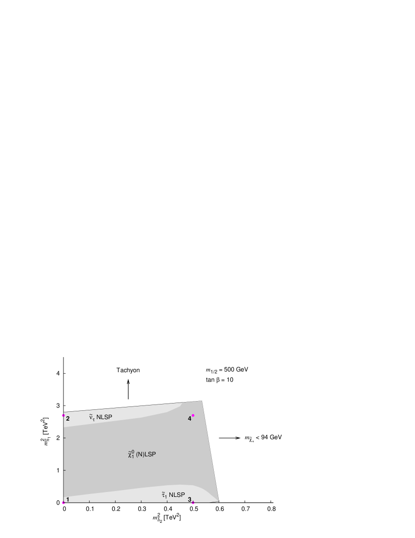
Figure 1: Allowed region for the soft Higgs masses. In the dark-gray area, a neutralino is lighter than all sleptons. For the points marked by the coloured dots, the resulting superparticle mass spectrum is shown in Fig. 3.

5.3 Dependence of the Spectrum on the Higgs Masses

Due to the large effects of the strong interaction, the squark masses experience the fastest running and end up around a TeV. The lighter stop mass runs more slowly due to $X_{t}$, which is always sizable at lower energies, and reaches a value of about $800{\,\text{Ge}\kern-0.66666pt\text{V\/}}$. If all scalar soft masses vanish at the GUT scale, the left-handed slepton masses change significantly in the beginning, but afterwards the evolution flattens as $g_{1}^{2}M_{1}^{2}$ and $g_{2}^{2}M_{2}^{2}$ decrease (cf. Eq. (39a)). Hence, they reach intermediate values between $300$ and $400{\,\text{Ge}\kern-0.66666pt\text{V\/}}$ at low energies. The flattening of the evolution is even more pronounced for the right-handed slepton masses, since here it depends only on $g_{1}^{2}M_{1}^{2}$, which decreases faster than $g_{2}^{2}M_{2}^{2}$. As a consequence, these scalars remain lighter than the lightest neutralino [9], which is approximately the bino: $m_{\tilde{e}_{\mathrm{R}}}(M_{Z})\simeq 180{\,\text{Ge}\kern-0.66666pt\text{V\/}}$, $m_{\chi^{0}_{1}}\simeq 200{\,\text{Ge}\kern-0.66666pt\text{V\/}}$. For both slepton “chiralities”, the third generation is slightly lighter than the first two due to $X_{\tau}$.

For $m^{2}_{\tilde{h}_{1}}\neq m^{2}_{\tilde{h}_{2}}$, the term involving $\operatorname{Tr}(Ym^{2})$ is non-vanishing and can lead to important changes [26, 10, 27, 28]. We shall first consider the case where it is negative ($m^{2}_{\tilde{h}_{1}}>m^{2}_{\tilde{h}_{2}}$) and saturates the bound from Eq. (41) (numerically, we find a slightly stronger bound of $m^{2}_{\tilde{h}_{1}}-m^{2}_{\tilde{h}_{2}}<2.7{\,\text{Te}\kern-0.66666pt\text{V\/}}^{2}$, which we use here). Then $|\operatorname{Tr}(Ym^{2})/m_{1/2}^{2}|\sim 10$, so that the first and second terms on the r.h.s. of the RGEs (35b) – (35f) can be of the same order of magnitude. An example for the running of the scalar masses is shown in Fig. 2.

Figure 2: Evolution of the scalar soft masses for $m^{2}_{\tilde{h}_{1}}=2.7{\,\text{Te}\kern-0.66666pt\text{V\/}}^{2}$, $m^{2}_{\tilde{h}_{2}}=0$ (point 2 in Fig. 1), $m_{1/2}=500{\,\text{Ge}\kern-0.66666pt\text{V\/}}$, $\tan\beta=10$ and $\text{sign}(\mu)=+1$ at $M_{\mathrm{GUT}}$.

The most drastic change occurs in the slepton spectrum. For the largest possible value of $\operatorname{Tr}(Ym^{2})$, the r.h.s. of Eq. (35e) vanishes exactly at the GUT scale. It turns negative only at lower energies due to the fast decrease of $|\operatorname{Tr}(Ym^{2})|$ (cf. Eq. (39b)). As a result, the left-handed sleptons remain relatively light, with a low-energy mass below $200{\,\text{Ge}\kern-0.66666pt\text{V\/}}$. Contrary to that, both terms in the RGE for the right-handed slepton masses are of the same sign, leading to an unusually fast running near the GUT scale. At lower energies, the evolution slows down quickly due to the fast decrease of both $g_{1}^{2}M_{1}^{2}$ and $|\operatorname{Tr}(Ym^{2})|$. The resulting masses are close to $400{\,\text{Ge}\kern-0.66666pt\text{V\/}}$. Thus, the NLSP is a sneutrino in this case [27], with a slightly heavier stau $\tilde{\tau}_{1}$ due to the $SU(2)_{\mathrm{L}}$ and $U(1)_{\mathrm{Y}}$ $D$-terms.

In the squark sector, large masses are generated again due to the strong interaction. At high energies, there is a significant cancellation in the RGE (35c) for the right-handed up-type squark masses, while the contributions to the other squark mass RGEs add up. Consequently, $m_{\tilde{u}_{\mathrm{R}}}$ and $m_{\tilde{t}_{\mathrm{R}}}$ run quite slowly until $|\operatorname{Tr}(Ym^{2})|$ has decreased sufficiently. Afterwards, $m_{\tilde{u}_{\mathrm{R}}}$ runs faster and comes close to the masses of the left-handed and right-handed down-type squarks at the electroweak scale.

If $m^{2}_{\tilde{h}_{1}}$ is neither close to zero nor to its upper bound, the running of the right-handed slepton masses is sufficiently enhanced to lift them above the lightest neutralino mass. At the same time, the running of the left-handed slepton masses is damped weakly enough, so that they are heavier than the lightest neutralino, too [10, 27]. A neutralino NLSP together with a gravitino LSP heavier than a GeV is excluded by cosmology [29, 31]. Therefore, this case is only viable if the neutralino is the LSP and the gravitino is heavier. This is possible, because we only have a lower bound on the gravitino mass. The corresponding region in parameter space is marked by the dark-gray area in Fig. 1. It grows for large values of $m^{2}_{\tilde{h}_{2}}$, since then mixing additionally decreases the lightest neutralino mass. A neutralino LSP is also often obtained if the compactification scale is larger than the unification scale. In this case, the running above $M_{\mathrm{GUT}}$ tends to make the sleptons heavier than the lightest neutralino [28, 34].

For $m^{2}_{\tilde{h}_{2}}>m^{2}_{\tilde{h}_{1}}$, $\operatorname{Tr}(Ym^{2})$ is positive. Now the evolution of the right-handed slepton masses is slowed down by the $\operatorname{Tr}(Ym^{2})$-term, while that of the left-handed masses is enhanced. Consequently, the NLSP is the predominantly right-handed $\tilde{\tau}_{1}$, with a mass of about $100{\,\text{Ge}\kern-0.66666pt\text{V\/}}$ for $m^{2}_{\tilde{h}_{2}}=0.5{\,\text{Te}\kern-0.66666pt\text{V\/}}^{2}$ and $m^{2}_{\tilde{h}_{1}}=0$. For these values, the masses of the left-handed sleptons are roughly $350{\,\text{Ge}\kern-0.66666pt\text{V\/}}$.

Since $m^{2}_{\tilde{h}_{2}}$ cannot be much larger than $0.5{\,\text{Te}\kern-0.66666pt\text{V\/}}^{2}$, the RGEs for the squark masses are always dominated by the term proportional to $g_{3}^{2}M_{3}^{2}$. Consequently, the low-energy masses are almost unchanged compared to the case of vanishing soft scalar masses at the compactification scale, except for $m_{\tilde{q}_{3\mathrm{L}}}$ and $m_{\tilde{t}_{\mathrm{R}}}$, which decrease by up to $60{\,\text{Ge}\kern-0.66666pt\text{V\/}}$ due to the larger $X_{t}$.

As the dominant parts of the RGEs depend only on the difference $m^{2}_{\tilde{h}_{1}}-m^{2}_{\tilde{h}_{2}}$, the same is true for the spectrum to a good approximation. The sum is only relevant for those third-generation masses whose evolution is sensitive to the $X_{i}$, most notably $m_{\tilde{t}_{\mathrm{R}}}$. In Fig. 3, we show the superparticle spectra that we obtain at the four points in parameter space marked by the coloured dots in Fig. 1.

Figure 3: Spectra of superparticle pole masses. The numbers at the bottom correspond to the points in parameter space marked by the coloured dots in Fig. 1. The high-energy boundary conditions for the soft Higgs masses were $m^{2}_{\tilde{h}_{1}}=m^{2}_{\tilde{h}_{2}}=0$ (point 1), $m^{2}_{\tilde{h}_{1}}=2.7{\,\text{Te}\kern-0.66666pt\text{V\/}}^{2}$, $m^{2}_{\tilde{h}_{2}}=0$ (point 2), $m^{2}_{\tilde{h}_{1}}=0$, $m^{2}_{\tilde{h}_{2}}=0.5{\,\text{Te}\kern-0.66666pt\text{V\/}}^{2}$ (point 3), and $m^{2}_{\tilde{h}_{1}}=2.7{\,\text{Te}\kern-0.66666pt\text{V\/}}^{2}$, $m^{2}_{\tilde{h}_{2}}=0.5{\,\text{Te}\kern-0.66666pt\text{V\/}}^{2}$ (point 4), respectively. In all cases, we used $m_{1/2}=500{\,\text{Ge}\kern-0.66666pt\text{V\/}}$, $\tan\beta=10$ and $\text{sign}(\mu)=+1$. As the first and second generation scalars are degenerate, only the first generation is listed in the figure. Particles with a mass difference of less than about $3{\,\text{Ge}\kern-0.66666pt\text{V\/}}$ are represented by a single line. The heavier neutralinos and the charginos have been omitted for better readability.

5.4 Dependence on the Gaugino Masses

To a first approximation, varying the high-energy gaugino mass simply leads to a rescaling of the scalar spectrum. If $m_{1/2}$ is increased while keeping the other soft masses fixed, the relative sizes of $\operatorname{Tr}(Ym^{2})$ and the $X_{i}$ decrease. Hence, they become less important and the spectrum comes closer to the one obtained in the minimal case of vanishing scalar masses.

As mentioned before, the LEP bound on the lightest Higgs mass leads to a lower bound on $m_{1/2}$. Actually, with our benchmark value $m_{1/2}=500{\,\text{Ge}\kern-0.66666pt\text{V\/}}$ we obtain a Higgs mass slightly below $114{\,\text{Ge}\kern-0.66666pt\text{V\/}}$ for small soft masses. However, the mass can easily be pushed beyond the bound by raising the top mass by about $1.5{\,\text{Ge}\kern-0.66666pt\text{V\/}}$ above its present best-fit value of $172.7{\,\text{Ge}\kern-0.66666pt\text{V\/}}$. Furthermore, a non-zero mass $m^{2}_{\tilde{h}_{1}}$ also causes an increase of the Higgs mass. If $m^{2}_{\tilde{h}_{1}}$ takes the maximal value allowed by Eq. (41), a unified gaugino mass of slightly less than $400{\,\text{Ge}\kern-0.66666pt\text{V\/}}$ is compatible with the LEP bound (for $m_{t}=172.7{\,\text{Ge}\kern-0.66666pt\text{V\/}}$).

5.5 Dependence on $\boldsymbol{\tan\beta}$

The influence of $\tan\beta$ on the results is also rather straightforward to understand. As to the RGEs, it only enters in the parameters $X_{t}$, $X_{b}$ and $X_{\tau}$, which play a role in the evolution of the third-generation soft masses. Hence, a change of $\tan\beta$ leads to a change of the mass splitting between this generation and the first two.

If $\tan\beta$ is significantly smaller than 10, the value used in our benchmark scenario, $X_{t}$ increases. Consequently, $\tilde{t}_{\mathrm{R}}$ and $\tilde{q}_{3\mathrm{L}}$ become slightly lighter. On the other hand, $X_{b}$ and $X_{\tau}$ are negligible now, so that the inter-generation mass splitting in the slepton and right-handed down-type squark sector becomes tiny. The Higgs mass bound leads to severer restrictions now. If $\tan\beta<8$, raising the top mass to the maximal value of $175.6{\,\text{Ge}\kern-0.66666pt\text{V\/}}$ allowed by experiment no longer yields $m_{h^{0}}>114.4{\,\text{Ge}\kern-0.66666pt\text{V\/}}$ for $m^{2}_{\tilde{h}_{1}}=0$. If $\tan\beta<6$, the bound is violated even for maximal $m_{t}$ and $m^{2}_{\tilde{h}_{1}}$, i.e. a gaugino mass larger than $500{\,\text{Ge}\kern-0.66666pt\text{V\/}}$ is required.

For larger values of $\tan\beta$, $X_{b}$ and $X_{\tau}$ become more important. Nevertheless, the impact of the former parameter on the RG evolution remains subdominant compared to that of the strong interaction. Hence, its increase only causes a larger splitting between $m_{\tilde{d}_{\mathrm{R}}}$ and $m_{\tilde{b}_{\mathrm{R}}}$, but does not lead to any new restrictions. In contrast, the lighter stau mass decreases a lot faster at lower energies due to the larger $X_{\tau}$. On the one hand, this increases the parameter space region where the $\tilde{\tau}_{1}$ is lighter than the neutralinos, as shown in Fig. 4 for $\tan\beta=20$. On the other hand, the soft scalar masses have to satisfy severer upper bounds in order to avoid tachyons and a too light stau.

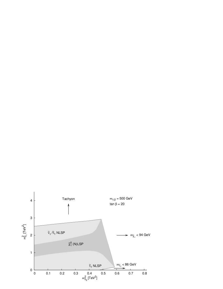
Figure 4: Allowed region for the soft Higgs masses for $\tan\beta=20$. In the dark-gray area, a neutralino is lighter than all sleptons.

As $\tan\beta$ increases beyond 20, mixing causes an additional decrease of $m_{\tilde{\tau}_{1}}$, as the off-diagonal term in the mass matrix, $\left(m^{2}_{\tilde{\tau}}\right)_{12}\simeq-v\mu y_{\tau}$, becomes comparable to the diagonal entries. For $\tan\beta=25$, the region of parameter space where the neutralino is lighter than the $\tilde{\tau}_{1}$ almost vanishes. For $\tan\beta=35$, the model is only viable if all soft scalar masses vanish at the GUT scale, and for $\tan\beta>35$ the lighter stau mass always lies below its experimental limit.

These problems are alleviated for heavier gauginos. In order to obtain a viable model with $\tan\beta=50$, one requires $m_{1/2}\gtrsim 850{\,\text{Ge}\kern-0.66666pt\text{V\/}}$, if all other soft masses vanish. If they are non-zero, the gaugino mass has to be even larger. In the resulting spectrum, only one stau is relatively light, while the remaining superparticle masses lie above $300{\,\text{Ge}\kern-0.66666pt\text{V\/}}$. As the lower bound on the gravitino mass rises with $m_{1/2}$, the gravitino may become heavier than the stau, which is excluded by cosmology.

We conclude that the model favours $10\lesssim\tan\beta\lesssim 25$. For values far outside this range, the phenomenological bounds on the soft masses are much more restrictive than the NDA limits, which appears unnatural.

6 Conclusions

We have discussed gaugino-mediated SUSY breaking in a six-dimensional $SO(10)$ orbifold GUT model where quarks and leptons are mixtures of brane and bulk fields. The couplings of bulk matter fields to the SUSY breaking gauge singlet brane field have to be suppressed in order to avoid large FCNCs. The compatibility of the SUSY breaking mechanism and orbifold GUTs with brane and bulk matter fields is a generic problem which requires further studies. We have also determined bounds on the SUSY breaking parameters by naïve dimensional analysis, which turn out not to restrict the phenomenologically allowed parameter regions.

The parameters relevant for the superparticle mass spectrum are the universal gaugino mass, the soft Higgs masses, $\tan\beta$ and the sign of $\mu$. We have analysed their impact on the spectrum and determined the region in parameter space that results in a viable phenomenology. The model favours moderate values of $\tan\beta$ between about 10 and 25. The gaugino mass at the GUT scale should not be far below $500{\,\text{Ge}\kern-0.66666pt\text{V\/}}$ in order to satisfy the LEP bound on the Higgs mass. Typically, the lightest neutralino is bino-like with a mass of $200{\,\text{Ge}\kern-0.66666pt\text{V\/}}$, and the gluino mass is about $1.2{\,\text{Te}\kern-0.66666pt\text{V\/}}$. Either the right-handed or the left-handed sleptons can be lighter than the neutralinos. The corresponding region in parameter space grows with $\tan\beta$. In this region, the gravitino is the LSP with a mass around $50{\,\text{Ge}\kern-0.66666pt\text{V\/}}$. The $\tilde{\tau}_{1}$ or the $\tilde{\nu}_{\tau\mathrm{L}}$ is the NLSP. A sneutrino NLSP has the advantage that constraints from big bang nucleosynthesis and the cosmic microwave background are less stringent [29]. For a stau NLSP, on the other hand, there exists the exciting possibility that its decays may lead to the discovery of the gravitino in future collider experiments [35].

References

• [1] Y. Kawamura, Prog. Theor. Phys. 103 (2000), 613 [hep-ph/9902423]
• [2] Y. Kawamura, Prog. Theor. Phys. 105 (2001), 999 [hep-ph/0012125]
• [3] G. Altarelli, F. Feruglio, Phys. Lett. B511 (2001), 257 [hep-ph/0102301]
• [4] L. J. Hall, Y. Nomura, Phys. Rev. D64 (2001), 055003 [hep-ph/0103125]
• [5] A. Hebecker, J. March-Russell, Nucl. Phys. B613 (2001), 3 [hep-ph/0106166]
• [6] T. Asaka, W. Buchmüller, L. Covi, Phys. Lett. B523 (2001), 199 [hep-ph/0108021]
• [7] L. J. Hall, Y. Nomura, T. Okui, D. R. Smith, Phys. Rev. D65 (2002), 035008 [hep-ph/0108071]
• [8] T. Asaka, W. Buchmüller, L. Covi, Phys. Lett. B563 (2003), 209 [hep-ph/0304142]
• [9] D. E. Kaplan, G. D. Kribs, M. Schmaltz, Phys. Rev. D62 (2000), 035010 [hep-ph/9911293]
• [10] Z. Chacko, M. A. Luty, A. E. Nelson, E. Ponton, JHEP 01 (2000), 003 [hep-ph/9911323]
• [11] T. Asaka, W. Buchmüller, L. Covi, Phys. Lett. B540 (2002), 295 [hep-ph/0204358]
• [12] G. F. Giudice, A. Masiero, Phys. Lett. B206 (1988), 480
• [13] M. Drees, Phys. Lett. B181 (1986), 279
• [14] C. F. Kolda, S. P. Martin, Phys. Rev. D53 (1996), 3871 [hep-ph/9503445]
• [15] W. Buchmüller, L. Covi, D. Emmanuel-Costa, S. Wiesenfeldt, JHEP 09 (2004), 004 [hep-ph/0407070]
• [16] W. Buchmüller, K. Hamaguchi, O. Lebedev, M. Ratz, hep-ph/0511035
• [17] Z. Chacko, M. A. Luty, E. Ponton, JHEP 07 (2000), 036 [hep-ph/9909248]
• [18] W. Buchmüller, K. Hamaguchi, J. Kersten, Phys. Lett. B632 (2006), 366 [hep-ph/0506105]
• [19] J. R. Ellis, C. Kounnas, D. V. Nanopoulos, Nucl. Phys. B247 (1984), 373
• [20] K. Inoue, M. Kawasaki, M. Yamaguchi, T. Yanagida, Phys. Rev. D45 (1992), 328
• [21] CDF Collaboration, D0 Collaboration, Tevatron Electroweak Working Group, hep-ex/0507091
• [22] B. C. Allanach, Comput. Phys. Commun. 143 (2002), 305 [hep-ph/0104145]
• [23] K. Inoue, A. Kakuto, H. Komatsu, S. Takeshita, Prog. Theor. Phys. 68 (1982), 927
• [24] K. Inoue, A. Kakuto, H. Komatsu, S. Takeshita, Prog. Theor. Phys. 71 (1984), 413
• [25] Particle Data Group, S. Eidelman et al., Phys. Lett. B592 (2004), 1
• [26] A. Lleyda, C. Muñoz, Phys. Lett. B317 (1993), 82 [hep-ph/9308208]
• [27] D. E. Kaplan, T. M. P. Tait, JHEP 06 (2000), 020 [hep-ph/0004200]
• [28] M. Schmaltz, W. Skiba, Phys. Rev. D62 (2000), 095004 [hep-ph/0004210]
• [29] M. Fujii, M. Ibe, T. Yanagida, Phys. Lett. B579 (2004), 6 [hep-ph/0310142]
• [30] J. L. Feng, S. Su, F. Takayama, Phys. Rev. D70 (2004), 075019 [hep-ph/0404231]
• [31] J. R. Ellis, K. A. Olive, Y. Santoso, V. C. Spanos, Phys. Lett. B588 (2004), 7 [hep-ph/0312262]
• [32] M. Kawasaki, K. Kohri, T. Moroi, Phys. Rev. D71 (2005), 083502 [astro-ph/0408426]
• [33] D. G. Cerdeño, K.-Y. Choi, K. Jedamzik, L. Roszkowski, R. Ruiz de Austri, hep-ph/0509275
• [34] H. Baer, A. Belyaev, T. Krupovnickas, X. Tata, Phys. Rev. D65 (2002), 075024 [hep-ph/0110270]
• [35] W. Buchmüller, K. Hamaguchi, M. Ratz, T. Yanagida, Phys. Lett. B588 (2004), 90 [hep-ph/0402179]
• [36] A. Brandenburg, L. Covi, K. Hamaguchi, L. Roszkowski, F. D. Steffen, Phys. Lett. B617 (2005), 99 [hep-ph/0501287].