Comparison of Boltzmann Equations with
Quantum Dynamics for Scalar Fields

Abstract

Boltzmann equations are often used to study the thermal evolution of particle reaction networks. Prominent examples are the computation of the baryon asymmetry of the universe and the evolution of the quark-gluon plasma after relativistic heavy ion collisions. However, Boltzmann equations are only a classical approximation of the quantum thermalization process which is described by the so-called Kadanoff-Baym equations. This raises the question how reliable Boltzmann equations are as approximations to the full Kadanoff-Baym equations. Therefore, we present in this paper a detailed comparison between the Kadanoff-Baym and Boltzmann equations in the framework of a scalar $\Phi^{4}$ quantum field theory in 3+1 space-time dimensions. The obtained numerical solutions reveal significant discrepancies in the results predicted by both types of equations. Apart from quantitative discrepancies, on a qualitative level the universality respected by the Kadanoff-Baym equations is severely restricted in the case of Boltzmann equations. Furthermore, the Kadanoff-Baym equations strongly separate the time scales between kinetic and chemical equilibration. This separation of time scales is absent for the Boltzmann equation.

I Introduction

One of the most attractive frameworks to explain the matter-antimatter asymmetry of the universe is the so-called leptogenesis mechanism Fukugita:1986hr ; Buchmuller:2004nz ; Buchmuller:2000nd . Here, lepton number violating interactions in the early universe produce a lepton asymmetry which is subsequently converted to the observed baryon asymmetry by so-called sphaleron processes. For the dynamical generation of the lepton asymmetry it is necessary, that the universe was in a state out of thermal equilibrium Sakharov:1967dj . The standard means to deal with this nonequilibrium situation are Boltzmann equations. However, it is well known that (classical) Boltzmann equations suffer from several shortcomings as compared to their quantum mechanical generalizations, the so-called Kadanoff-Baym equations. This motivates a comparison of Boltzmann and Kadanoff-Baym equations in order to assess the reliability of quantitative predictions of leptogenesis scenarios.

In addition to leptogenesis, there are various other systems which warrant a comparison between Boltzmann and Kadanoff-Baym equations: In particular, a strong motivation is furnished by relativistic heavy ion collision experiments which aim at testing the quark-gluon plasma. In these experiments the quark-gluon plasma is produced in a state far from equilibrium. Recently, however, experiments claimed that the approach to thermal equilibrium should happen very fast, and that the evolution of the quark-gluon plasma could even be described by hydrodynamic equations Arsene:2004fa ; Back:2004je ; Adams:2005dq ; Adcox:2004mh , which arise as approximations to Boltzmann equations. In this context it is important to note that different quantities effectively thermalize on different time scales Berges:2004ce . Thus, one might face the situation that, although the full approach to thermal equilibrium takes a very long time, certain quantities, which are sufficient to describe the quark-gluon plasma with hydrodynamic equations, approach equilibrium values on much shorter time scales.

In order to derive Boltzmann equations from Kadanoff-Baym equations, one has to employ several approximations, among them a first-order gradient expansion, a Wigner transformation and a quasi-particle (or on-shell) approximation baymKadanoff1962a ; Danielewicz:1982kk ; Ivanov:1999tj ; Knoll:2001jx ; Blaizot:2001nr . However, it is known, that the gradient expansion cannot be justified for early times. Consequently, one might expect that Boltzmann equations fail to describe the early-time evolution and that errors accumulated for early times cannot be remedied at late times. Of course, a Wigner transformation itself is not at all an approximation, but in order to make it available, one has to send the initial time to the remote past. Whereas Boltzmann equations imply the assumption of molecular chaos, meaning that two particles were uncorrelated before their collision, Kadanoff-Baym equations take these memory effects into account. Numerical solutions of Kadanoff-Baym equations revealed that this memory is lost gradually. Consequently, for late times it is indeed justifiable to send the initial time to the remote past. However, for early times this is certainly not the case. Furthermore, as a consequence of the quasi-particle approximation, the conservation of momentum and energy prevents Boltzmann equations from describing thermalization in $1+1$ space-time dimensions. In contrast to this, it has been shown in the framework of a scalar $\Phi^{4}$ quantum field theory that this is feasible with Kadanoff-Baym equations Berges:2001fi . The reason for this qualitative discrepancy is that Kadanoff-Baym equations take off-shell effects into account Aarts:2001qa , which are neglected in Boltzmann equations. Of course, in 3+1 dimensions both types of equations are capable of describing thermalization. In the case of leptogenesis, however, the on-shell character of the Boltzmann equation leads to a further inconsistency: All leptogenesis scenarios share the fact that some heavy particles decay out of thermal equilibrium into the particles which we observe in the universe today. The spectral function of a particle that can decay into other particles is given by a Breit-Wigner curve with a non-vanishing width. By employing the quasi-particle approximation we reduce this decay width of the particles to zero, i.e. a Boltzmann equation can only describe systems consisting of stable, or at least very long-lived, particles. After all, how does the on-shell character of the Boltzmann equation affect the description of quantum fields out of thermal equilibrium in $3+1$ dimensions?

When applying Boltzmann equations to the description of leptogenesis, the standard technique to construct the collision integrals — before employing further approximations — is to take the usual bosonic and fermionic statistical gain and loss terms multiplied with the S-matrix element for the respective reaction Kolb:1979qa ; kolbTurner1990a . These S-matrix elements are computed in vacuum, and one may wonder of which significance they are for a statistical quantum mechanical system.

All these shortcomings of Boltzmann equations lead to the conclusion that one should perform a detailed comparison between Boltzmann and Kadanoff-Baym equations Danielewicz:1982kk ; kohler1995a ; Morawetz:1998em ; Juchem:2003bi , such that one can explicitely see how large the quantum mechanical corrections are. Due to the complexity of the problem, we restrict ourselves for the moment to a $\Phi^{4}$ quantum field theory in $3+1$ space-time dimensions. Of course, in this framework one can neither describe the phenomenon of leptogenesis nor thermalization after a heavy ion collision. Nevertheless, it may well serve as starting point for further research, and certainly permits to present a detailed comparison between Boltzmann and Kadanoff-Baym equations, which may point to interesting phenomena to be investigated in more realistic theories.

In general, when studying systems out of thermal equilibrium by means of Kadanoff-Baym equations, it is crucial to start from a $\Phi$-derivable approximation, since these approximations ensure the conservation of energy and global charges baymKadanoff1961a ; Baym:1962sx ; Ivanov:1998nv . The 2PI effective action furnishes such a $\Phi$-derivable approximation Jackiw:1974cv ; Cornwall:1974vz ; Calzetta:1986cq and has proven to be an efficient and reliable tool for the description of out-of-equilibrium quantum fields in numerous previous treatments Berges:2000ur ; Berges:2001fi ; Berges:2002wr ; Aarts:2001yn ; Aarts:2003bk ; Berges:2004hn . In this work, we start from the 2PI effective action truncated at three-loop order. The Kadanoff-Baym equations can be obtained by requiring that the 2PI effective action be stationary with respect to variations of the full connected two-point function Aarts:2001qa ; Berges:2001fi . In order to derive the corresponding Boltzmann equation, subsequently one has to employ a gradient expansion, a Wigner transformation, the Kadanoff-Baym ansatz and the quasi-particle approximation baymKadanoff1962a ; Danielewicz:1982kk ; Ivanov:1999tj ; Knoll:2001jx ; Blaizot:2001nr . While the Boltzmann equation describes the time evolution of the particle number distribution, the Kadanoff-Baym equations describe the evolution of the full quantum mechanical two-point function of the system. However, one can define an effective particle number distribution which is given by the full propagator and its time derivatives evaluated at equal times Berges:2001fi ; Berges:2002wr . Finally, we solve the Boltzmann and the Kadanoff-Baym equations numerically for spatially homogeneous and isotropic systems in 3+1 dimensions and compare their predictions on the evolution of these systems for various initial conditions.

II 2PI Effective Action

In this work we consider a real scalar quantum field, whose dynamics is determined by the Lagrangian density

$$\mathscr{L}=-\frac{1}{2}\Big{(}\partial_{\mu}\Phi\Big{)}\Big{(}\partial^{\mu}\Phi\Big{)}-\frac{1}{2}m_{B}^{2}\Phi^{2}-\frac{\lambda}{4!}\Phi^{4}\;.$$

The minus sign of the kinetic term indicates that we use the metric where the time-time component is negative. As we will compute the evolution of the two-point Green’s function for a nonequilibrium many body system, already the classical action has to be defined on the closed Schwinger-Keldysh real-time contour, shown in Fig. 1.

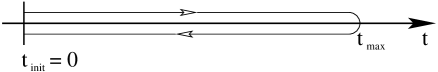
Figure 1: Closed real-time path $\mathcal{C}$. This time path was invented by Schwinger Schwinger:1960qe (see also Bakshi:1962dv ; Bakshi:1963bn ) and applied to nonequilibrium problems by Keldysh Keldysh:1964ud . In order to avoid the doubling of the degrees of freedom, we use the form presented in Ref. Danielewicz:1982kk .

The free inverse propagator can then be read off the free part of the classical action

$$I_{0}=-\frac{1}{2}\int\limits_{\mathcal{C}}d^{4}x\int\limits_{\mathcal{C}}d^{4}y\left[\Phi\left(x\right)G_{0}^{-1}\left(x,y\right)\Phi\left(y\right)\right]\;,$$

where

$$G_{0}^{-1}\left(x,y\right)=\left(\partial_{x^{\mu}}\partial_{y_{\mu}}+m_{B}^{2}\right)\delta_{\mathcal{C}}\left(x-y\right)\;.$$ (1)

We consider a system without symmetry breaking, i.e. $\left\langle\Phi\left(x\right)\right\rangle=0$. In this case the full connected Schwinger-Keldysh propagator is given by

$$G\left(x,y\right)=\left\langle T_{\mathcal{C}}\left\{\Phi\left(x\right)\Phi\left(y\right)\right\}\right\rangle\;.$$

Accordingly, for Gaussian initial conditions the 2PI effective action can be parameterized in the form Jackiw:1974cv ; Cornwall:1974vz ; Calzetta:1986cq ; Berges:2001fi

$$\Gamma\left[G\right]=\frac{i}{2}\mbox{tr}_{\mathcal{C}}\log_{\mathcal{C}}\left[G^{-1}\right]-\frac{1}{2}\mbox{tr}_{\mathcal{C}}\left[G_{0}^{-1}G\right]+\Gamma_{2}\left[G\right]+const\;.$$

$i\Gamma_{2}\left[G\right]$ is the sum of all two-particle irreducible vacuum diagrams, where internal lines represent the full connected propagator $G\left(x,y\right)$. Of course, for an interacting theory we cannot compute $\Gamma_{2}\left[G\right]$ completely, and we have to rely on approximations. In this work we apply the loop expansion of the 2PI effective action up to three-loop order. The diagrams contributing to $\Gamma_{2}\left[G\right]$ in this approximation are shown in Fig. 2. We find Aarts:2001qa :

$$\Gamma_{2}\left[G\right] = -\frac{\lambda}{8}\int\limits_{\mathcal{C}}d^{4}x\left[G\left(x,x\right)G\left(x,x\right)\right]$$

$${}+\frac{i\lambda^{2}}{48}\int\limits_{\mathcal{C}}d^{4}x\int\limits_{\mathcal{C}}d^{4}y\left[G\left(x,y\right)G\left(x,y\right)G\left(y,x\right)G\left(y,x\right)\right]\;.$$

III Kadanoff-Baym Equations

The equation of motion for the full propagator reads Jackiw:1974cv ; Cornwall:1974vz

$$\frac{\delta\Gamma\left[G\right]}{\delta G\left(y,x\right)}=0\;.$$

It is equivalent to the Schwinger-Dyson equation

$$G^{-1}\left(x,y\right)=iG^{-1}_{0}\left(x,y\right)-\Pi\left(x,y\right)\;,$$ (2)

where the proper self energy is given by

$$\Pi\left(x,y\right)=2i\frac{\delta\Gamma_{2}\left[G\right]}{\delta G\left(y,x\right)}=-\frac{i\lambda}{2}\delta_{\mathcal{C}}\left(x-y\right)G\left(x,x\right)-\frac{\lambda^{2}}{6}G\left(x,y\right)G\left(x,y\right)G\left(y,x\right)\;.$$ (3)

After we have inserted the free inverse propagator given in Eq. (1), we convolute the Schwinger-Dyson equation (2) with $G$ from the right:

Figure 2: Two- and three-loop contribution to $\Gamma_{2}\left[G\right]$. The lines represent the full connected Schwinger-Keldysh propagator.

$$i\left(-\partial_{x^{\mu}}\partial_{x_{\mu}}+m_{B}^{2}\right)G\left(x,y\right)=\delta_{\mathcal{C}}\left(x-y\right)+\int\limits_{\mathcal{C}}d^{4}z\left[\Pi\left(x,z\right)G\left(z,y\right)\right]$$ (4)

Next, we define the spectral function

$$G_{\varrho}\left(x,y\right)=i\left\langle\left[\Phi\left(x\right),\Phi\left(y\right)\right]_{-}\right\rangle$$

and the statistical propagator

$$G_{F}\left(x,y\right)=\frac{1}{2}\left\langle\left[\Phi\left(x\right),\Phi\left(y\right)\right]_{+}\right\rangle$$

such that we can write the full propagator as

$$G\left(x,y\right)=G_{F}\left(x,y\right)-\frac{i}{2}\mbox{sign}_{\mathcal{C}}\left(x^{0}-y^{0}\right)G_{\varrho}\left(x,y\right)\;.$$ (5)

Note that for real scalar quantum fields both the statistical propagator and the spectral function are real-valued functions Berges:2001fi . The spectral function describes the particle spectrum of our theory. From its Wigner transform we can obtain the thermal mass and the decay width of the particles in our system. On the other hand we will define an effective particle number density given by the statistical propagator and its time derivatives evaluated at equal times. From Eq. (3) (and Fig. 3) we see that the self energy contains a local and a nonlocal part:

$$\Pi\left(x,y\right)=-i\delta_{\mathcal{C}}\left(x-y\right)\Pi^{(local)}\left(x\right)+\Pi^{(nonlocal)}\left(x,y\right)\;.$$

The local part of the self energy only causes a mass shift, which can be included in an effective mass:

$$M^{2}\left(x\right)=m_{B}^{2}+\Pi^{(local)}\left(x\right)=m_{B}^{2}+\frac{\lambda}{2}G_{F}\left(x,x\right)\;.$$ (6)

After inserting Eq. (5) into Eq. (3), we can decompose the nonlocal part of the self energy in exactly the same way as we did for the propagator:

Figure 3: One- and two-loop contribution to the proper self-energy $\Pi$. Again, internal lines represent the full connected Schwinger-Keldysh propagator. The tadpole represents the local part which causes a mass shift only. The setting-sun diagram represents the nonlocal part and leads to thermalization.

$$\Pi^{(nonlocal)}\left(x,y\right)=\Pi_{F}\left(x,y\right)-\frac{i}{2}\mbox{sign}_{\mathcal{C}}\left(x^{0}-y^{0}\right)\Pi_{\varrho}\left(x,y\right)\;.$$

We find

$$\Pi_{F}\left(x,y\right)=-\frac{\lambda^{2}}{6}\Big{(}G_{F}\left(x,y\right)G_{F}\left(x,y\right)G_{F}\left(x,y\right)-\frac{3}{4}G_{\varrho}\left(x,y\right)G_{\varrho}\left(x,y\right)G_{F}\left(x,y\right)\Big{)}$$

and

$$\Pi_{\varrho}\left(x,y\right)=-\frac{\lambda^{2}}{6}\Big{(}3G_{F}\left(x,y\right)G_{F}\left(x,y\right)G_{\varrho}\left(x,y\right)-\frac{1}{4}G_{\varrho}\left(x,y\right)G_{\varrho}\left(x,y\right)G_{\varrho}\left(x,y\right)\Big{)}\;.$$

When we insert all these definitions into Eq. (4), we observe that it splits into two complementary real-valued evolution equations for the statistical propagator and the spectral function, respectively Berges:2001fi . These are the so-called Kadanoff-Baym equations:

$$\left(-\partial_{x^{\mu}}\partial_{x_{\mu}}+M^{2}\left(x\right)\right)G_{F}\left(x,y\right)=\int\limits_{0}^{y^{0}}d^{4}z\;\Pi_{F}\left(x,z\right)G_{\varrho}\left(z,y\right)-\int\limits_{0}^{x^{0}}d^{4}z\;\Pi_{\varrho}\left(x,z\right)G_{F}\left(z,y\right)$$ (7)

and

$$\left(-\partial_{x^{\mu}}\partial_{x_{\mu}}+M^{2}\left(x\right)\right)G_{\varrho}\left(x,y\right)=-\int\limits_{y^{0}}^{x^{0}}d^{4}z\;\Pi_{\varrho}\left(x,z\right)G_{\varrho}\left(z,y\right)\;.$$ (8)

For a spatially homogeneous system, one can Fourier transform these equations with respect to the spatial relative coordinate. Furthermore, in an isotropic system the propagator will depend only on the modulus of the momentum. As explained in more detail in Refs. Berges:2001fi ; Berges:2002wr , one can define effective kinetic energy and particle number densities $\omega\left(t,\bm{p}\right)$ and $n\left(t,\bm{p}\right)$ which are given by

$$\omega^{2}\left(t,\bm{p}\right)=\left(\frac{\partial_{x^{0}}\partial_{y^{0}}G_{F}\left(x^{0},y^{0},\bm{p}\right)}{G_{F}\left(x^{0},y^{0},\bm{p}\right)}\right)_{x^{0}=y^{0}=t}$$ (9)

and

$$n\left(t,\bm{p}\right)=\omega\left(t,\bm{p}\right)G_{F}\left(t,t,\bm{p}\right)-\frac{1}{2}\;.$$ (10)

However, we stress that the Kadanoff-Baym equations are self-consistent evolution equations for the full propagator of our system, and that one has to follow the evolution of the two-point function throughout the whole $x^{0}$-$y^{0}$-plane (of course, constrained to the part with $x^{0}\geq 0$ and $y^{0}\geq 0$). One can then follow the evolution of the effective particle number density along the bisecting line of this plane.

We would like to emphasize that the only approximation involved in the numerical solution of the Kadanoff-Baym equations is the loop expansion of the 2PI effective action. In the next section we will describe the approximations which are necessary to derive a Boltzmann equation from the Kadanoff-Baym equation for the statistical propagator (7).

IV Boltzmann Equations

It is well known how Boltzmann equations can be obtained as an approximation of the Kadanoff-Baym equations baymKadanoff1962a ; Danielewicz:1982kk ; Blaizot:2001nr . In this section we briefly review the standard derivation: One has to employ a Wigner transformation, a gradient expansion, the Kadanoff-Baym ansatz and the quasi-particle approximation.

First, we subtract the Hermitian adjoint of Eq. (7) from Eq. (7) and re-parameterize the propagator and the self energy by center and relative coordinates

$$G\left(u,v\right)=\tilde{G}\left(\frac{u+v}{2},u-v\right)\;.$$

Next, we define $X=\frac{x+y}{2}$ and $s=x-y$, and observe on the left hand side of the difference equation that

$$-\partial_{x^{\mu}}\partial_{x_{\mu}}+\partial_{y^{\mu}}\partial_{y_{\mu}}=-2\partial_{X^{\mu}}\partial_{s_{\mu}}$$

is automatically of first order in $\partial_{X}$. Furthermore, we Taylor expand the effective masses on the left hand side as well as the propagators and self energies on the right hand side to first order in $\partial_{X}$ around $X$. After that, we Fourier transform the difference equation with respect to $s$. The Wigner transformed statistical propagator and spectral function are given by

$$\tilde{G}_{F}\left(X,k\right)=\int d^{4}s\;\exp\left(-iks\right)\tilde{G}_{F}\left(X,s\right)$$

and

$$\tilde{G}_{\varrho}\left(X,k\right)=-i\int d^{4}s\;\exp\left(-iks\right)\tilde{G}_{\varrho}\left(X,s\right)\;.$$

The factor of $-i$ in the Wigner transform of the spectral function makes $\tilde{G}_{\varrho}\left(X,k\right)$ again a real-valued function. However, in order to be able to really perform the Fourier transformation, we have to send the initial time to $-\infty$. At least for large $x^{0}$ and $y^{0}$ this can be justified by taking into account that correlations between earlier and later times are suppressed exponentially, as one can see in Fig. 5.

Figure 4: The modulus of the unequal-time propagator as function of time for fixed momentum mode $\bm{p}=0$. Correlations between earlier and later times are exponentially damped.

Figure 5: The equal-time propagator as a function of time for three different initial conditions (cf. Fig. 6). The system shows rapid oscillations which die out after moderate times and are followed by a smooth drifting regime.

The result of all these transformations is a quantum kinetic equation for the statistical propagator Ivanov:1999tj ; Knoll:2001jx ; Blaizot:2001nr ; Berges:2002wt ; Juchem:2004cs ; Berges:2005vj ; Berges:2005md :

$$\left(2k^{\mu}\partial_{X^{\mu}}-\left(\partial_{X^{\mu}}M^{2}\left(X\right)\right)\partial_{k_{\mu}}\right)\tilde{G}_{F}\left(X,k\right)$$

$$= \tilde{\Pi}_{\varrho}\left(X,k\right)\tilde{G}_{F}\left(X,k\right)-\tilde{\Pi}_{F}\left(X,k\right)\tilde{G}_{\varrho}\left(X,k\right)$$

$${}+\left\{\tilde{\Pi}_{F}\left(X,k\right);\mbox{Re}\left(\tilde{G}_{R}\left(X,k\right)\right)\right\}_{PB}+\left\{\mbox{Re}\left(\tilde{\Pi}_{R}\left(X,k\right)\right);\tilde{G}_{F}\left(X,k\right)\right\}_{PB}\;,$$

where the Poisson brackets are defined by

$$\left\{\tilde{f}\left(X,k\right);\tilde{g}\left(X,k\right)\right\}_{PB}=\Big{[}\partial_{X^{\mu}}\tilde{f}\left(X,k\right)\Big{]}\Big{[}\partial_{k_{\mu}}\tilde{g}\left(X,k\right)\Big{]}-\Big{[}\partial_{k_{\mu}}\tilde{f}\left(X,k\right)\Big{]}\Big{[}\partial_{X^{\mu}}\tilde{g}\left(X,k\right)\Big{]}\;.$$ (12)

Employing the first order Taylor expansion is clearly not justifiable for early times when the equal-time propagator is rapidly oscillating, cf. Fig. 5. But this is obvious, since employing this gradient expansion is clearly motivated by equilibrium considerations: In equilibrium the propagator depends on the relative coordinates only. There is no dependence on the center coordinates, and one may hope that there are situations where the propagator depends only moderately on the center coordinates. This is clearly the case for late times when our system is sufficiently close to equilibrium. However, as is shown in Fig. 5, already after moderate times the rapid oscillations mentioned above, have died out and are followed by a smooth drifting regime Berges:2001fi . In this drifting regime the second derivative with respect to $X$ should be negligible as compared to the first order derivative and a consistent Taylor expansion can be justified even though the system may still be far from equilibrium. However, it is crucial that the Taylor expansion is performed consistently for two reasons: First, this guarantees that the quantum kinetic equations satisfy exactly the same conservation laws as the full Kadanoff-Baym equations do Knoll:2001jx . Second, it has been shown that neglecting the Poisson brackets severely restricts the range of validity of the quantum kinetic equations Berges:2005ai ; Berges:2005md . For the intermediate and late-time regimes these quantum kinetic equations have the advantage that they do not include any memory integrals. Being local in time, their numerical solution requires much less computer memory as compared to the Kadanoff-Baym equations and algorithms using an adaptively controlled time-step size become available. Furthermore, the energy convolutions replacing the memory integrals can be done quite efficiently using a Fast Fourier Transform algorithm. In order to derive a Boltzmann equation from the quantum kinetic equation (IV), first we have to discard the Poisson brackets, thereby sacrificing the consistency of the gradient expansion. After that, we employ the Kadanoff-Baym ansatz

$$\tilde{G}_{F}\left(X,k\right)=\tilde{G}_{\varrho}\left(X,k\right)\left(\tilde{n}\left(X,k\right)+\frac{1}{2}\right)\;,$$ (13)

which also can be motivated by equilibrium considerations. In fact, this is a generalization of the fluctuation-dissipation theorem, which states that, for a system in thermal equilibrium, the statistical propagator is proportional to the spectral function. The fluctuation dissipation theorem can be recovered from Eq. (13) by discarding the dependence on the center coordinate $X$ and fixing $\tilde{n}$ to be the Bose-Einstein distribution function. The last approximation, which is necessary to arrive at the Boltzmann equation, is the so-called quasi-particle (or on-shell) approximation:

$$\tilde{G}_{\varrho}\left(X,k\right)=\frac{\pi}{E\left(X,\bm{k}\right)}\Big{(}\delta\left(k^{0}-E\left(X,\bm{k}\right)\right)-\delta\left(k^{0}+E\left(X,\bm{k}\right)\right)\Big{)}\;,$$ (14)

where the quasi-particle energy is given by

$$E\left(X,\bm{k}\right)=\sqrt{m_{th}^{2}+\bm{k}^{2}}\;.$$

Once more, we would like to stress that the exact time evolution of the spectral function is determined by the Kadanoff-Baym equations. It has been shown that the spectral function can be parameterized by a Breit-Wigner function with a non-vanishing width Aarts:2001qa ; Juchem:2003bi . To reduce the width of this Breit-Wigner curve to zero is certainly not a controllable approximation and leads to significant qualitative discrepancies between the results produced by Kadanoff-Baym and Boltzmann equations. In fact this approximation can only be justified if our system consists of stable, or at least very long-lived, quasi-particles, whose mass is much larger than their decay width. We also would like to note that a completely self-consistent determination of the thermal mass in the framework of the Boltzmann equation requires the solution of an integral equation for $E\left(X,\bm{k}\right)$, which would drastically increase the complexity of our numerics. As none of our physical results depend on the exact value of the thermal mass, for convenience, we set $m_{th}$ to the equilibrium value of the thermal mass as determined by the Kadanoff-Baym equations. Eventually, we define the quasi-particle number density by

$$n\left(X,\bm{k}\right)=\tilde{n}\left(X,\bm{k},E\left(X,\bm{k}\right)\right)\;.$$

After equating the positive energy components in Eq. (IV) we arrive at the Boltzmann equation. For a spatially homogeneous system there is no dependence on the spatial center coordinates and the Boltzmann equation reads:

$$\partial_{t}n\left(t,\bm{k}\right)=\frac{\lambda^{2}\pi}{48}\int\frac{d^{3}p}{\left(2\pi\right)^{3}}\int\frac{d^{3}q}{\left(2\pi\right)^{3}}\int d^{3}r\Bigg{[}\frac{1}{E_{k}E_{p}E_{q}E_{r}}$$

$${}\times\delta\left(\bm{k}+\bm{p}-\bm{q}-\bm{r}\right)\delta\left(E_{k}+E_{p}-E_{q}-E_{r}\right)$$

$${}\times\Big{(}\left(1+n_{\bm{k}}\right)\left(1+n_{\bm{p}}\right)n_{\bm{q}}n_{\bm{r}}-n_{\bm{k}}n_{\bm{p}}\left(1+n_{\bm{q}}\right)\left(1+n_{\bm{r}}\right)\Big{)}\Bigg{]}\;.$$

For a spatially homogeneous and isotropic system we can dramatically simplify the collision integral Dolgov:1997mb , which allows us to reduce the complexity of our numerics significantly. The details of this calculation are shown in the appendix. The result is the following equation:

$$\partial_{t}n\left(t,k\right)=\frac{\lambda^{2}}{96\pi^{4}}\int\limits_{0}^{\infty}dp\int\limits_{0}^{\infty}dq\Bigg{[}\Theta\left(r_{0}^{2}\right)\frac{pqD\left(k,p,q,r_{0}\right)}{E_{k}E_{p}E_{q}}$$

$${}\times\Big{(}\left(1+n_{k}\right)\left(1+n_{p}\right)n_{q}n_{r_{0}}-n_{k}n_{p}\left(1+n_{q}\right)\left(1+n_{r_{0}}\right)\Big{)}\Bigg{]}\;.$$

The auxiliary functions $r_{0}$ and $D$ are obtained from very simple expressions which are given in the appendix. In this section we have shown that, using a gradient expansion and a quasi-particle (or on-shell) approximation, one can derive the Boltzmann equation from the Kadanoff-Baym equations. In this sense one can consider the Kadanoff-Baym equations as quantum Boltzmann equations re-summing the gradient expansion up to infinite order and including off-shell and memory effects. In the next section we are going to explain how we solved the Boltzmann and the Kadanoff-Baym equations numerically.

V Numerical Implementation

V.1 Kadanoff-Baym Equations

For the numerical solution of the Kadanoff-Baym equations we follow exactly the lines of Refs. Berges:2001fi ; Berges:2004yj ; montvayMunster1994a , i.e. for the spatial coordinates we employ a standard discretization on a three-dimensional lattice with lattice spacing $a_{s}$ and $N_{s}$ lattice sites in each direction. Thus, the lattice momenta are given by

$$\hat{p}_{n_{j}}=\frac{2}{a_{s}}\sin\left(\frac{\pi n_{j}}{N_{s}}\right)\;,$$

where $n_{j}$, $j\in\left\{1,2,3\right\}$, enumerates the momentum modes in the $j$-th dimension. As we consider a spatially homogeneous and isotropic system, for given times $\left(x^{0},y^{0}\right)$ we only need to store the propagator for momentum modes with $\frac{N_{s}}{2}\geq n_{1}\geq n_{2}\geq n_{3}\geq 0$. This saves us a factor of 48 in memory usage. The discretization in time leads to a history matrix $H=\left\{0,a_{t},2a_{t},\ldots,\left(N_{t}-1\right)a_{t}\right\}^{2}$. Here $a_{t}$ is the step size and $N_{t}$ is the number of times in each time dimension for which we keep the propagator in memory in order to compute the memory integrals. This history cut off can be justified by the exponential damping of the unequal-time propagator, cf. Fig. 5. Exploiting the symmetry of the statistical propagator with respect to the interchange of its time arguments, we only need to store the values of the statistical propagator for $x^{0}\geq y^{0}$. In very much the same way we can use the respective antisymmetry of the spectral function. This saves us another factor of 2 in memory usage. The convolutions arising in the computation of the setting-sun self-energies are most efficiently computed using a Fast Fourier Transform algorithm for real-valued even functions fftw .

In order to set the scale for the simulations, we use the renormalized vacuum mass $m_{R}$. The corresponding bare mass $m_{B}$ is obtained through a perturbative renormalization at one-loop order of the self energy (tadpole) Arrizabalaga:2005tf . We solved the Kadanoff-Baym equations numerically on a lattice with $N_{t}=500$, $N_{s}=32$, $a_{t}m_{R}=0.06$, $a_{s}m_{R}=0.5$ and $\lambda=18$. So far we performed our simulations on a simple desktop PC with a Pentium4 processor and 2 GByte RAM. However, we would like to note that the numerics can easily be parallelized.

V.2 Boltzmann Equation

As we saw in the previous paragraph, in order to discretize the Kadanoff-Baym equations we can rely on the well-defined scheme offered by standard lattice field theory. Unfortunately, the energy conserving $\delta$ function in Eq. (IV) prevents us from using these standard lattice techniques for the Boltzmann equation. The reason is the following: When integrating over an arbitrary momentum mode in Eq. (IV) one has to look for zeros of the argument of the energy conserving $\delta$ function with respect to this particular momentum mode. These zeros might well fall between two lattice sites. Hence, computing the collision integral requires the use of interpolation techniques in order to determine the particle number distribution for these in-between lattice sites. These interpolation techniques imply a continuity assumption for the particle number distribution which contradicts the strict lattice discretization as offered by lattice field theory. Apart from this principal obstacle, there is also a practical reason which encourages us to use different discretization schemes for both types of equations: The collision integral in Eq. (IV) is no convolution. Consequently, Fast Fourier Transformation algorithms are not applicable, and its numerical computation becomes rather expensive. In order to reduce the complexity of our Boltzmann numerics we exploited isotropy, which allowed us to simplify the Boltzmann equation analytically and lead us to Eq. (IV). In the discretized version of the Boltzmann equation (IV) the momenta are of the form

$$p_{n}=\frac{\sqrt{12}}{a_{s}N_{s}}n\;.$$

We use the same value for $a_{s}$ as for the Kadanoff-Baym equations. This ensures that the largest available momentum is the same as for the Kadanoff-Baym equations. Of course, $N_{s}$ need not be the same as for the Kadanoff-Baym equations, which just means that we approach the physically relevant infinite volume limit independently for both types of equations.

In order to compute the collision integral we proceed as follows: For fixed $\left(k,p,q\right)$ we determine $r_{0}$ (the exact definition of $r_{0}$ is given in the appendix), which of course need not be one of the discretized momenta given above. The function $D\left(k,p,q,r_{0}\right)$ can be evaluated for any value of $r_{0}$ (as one also can see in the appendix). To obtain the particle number density for an arbitrary $r_{0}$ we use a cubic spline interpolation gsl . Thus, for given $\left(k,p,q\right)$ the integrand is known to any given accuracy and for given $k$ we can simply sum over $p$ and $q$. In order to advance in time we use a Runge-Kutta-Cash-Karp routine with adaptive step-size control gsl .

In order to set the scale for the simulations, again we use the renormalized vacuum mass $m_{R}$. Our simulations were done with $N_{s}=500$, $a_{s}m_{R}=0.5$ and $\lambda=18$.

VI Comparing Boltzmann vs. Kadanoff-Baym

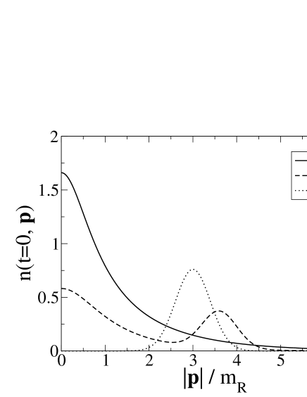
Figure 6: Initial particle number densities against absolute momenta. Shown are the three different initial conditions (IC) discussed in the text, for which we numerically solved the Boltzmann and the Kadanoff-Baym equations, respectively. All initial conditions correspond to the same (conserved) average energy density. Above that, the initial conditions IC1 and IC2 also correspond to the same initial average particle number density.

We consider three different initial conditions which correspond to the same average energy density. Above that, the initial conditions IC1 and IC2 also correspond to the same initial average particle number density. The corresponding initial particle number distributions are shown in Fig. 6. These particle number distributions can immediately be fed into the numerics for the Boltzmann equation. In order to obtain the initial conditions for the Kadanoff-Baym equations, we follow Refs. Berges:2001fi ; Berges:2002wr : The initial values for the spectral function are determined from the canonical commutation relations. On the other hand, for a given initial particle number density, the initial values for the statistical propagator and its derivatives are determined according to:

$$G_{F}\left(x^{0},y^{0},\bm{p}\right)_{x^{0}=y^{0}=0}=\left[\frac{n\left(t,\bm{p}\right)+\frac{1}{2}}{\omega\left(t,\bm{p}\right)}\right]_{t=0}\;,$$ (17)

$$\left[\partial_{x^{0}}G_{F}\left(x^{0},y^{0},\bm{p}\right)\right]_{x^{0}=y^{0}=0}=0\;,$$ (18)

$$\left[\partial_{x^{0}}\partial_{y^{0}}G_{F}\left(x^{0},y^{0},\bm{p}\right)\right]_{x^{0}=y^{0}=0}=\left[\omega\left(t,\bm{p}\right)\left(n\left(t,\bm{p}\right)+\frac{1}{2}\right)\right]_{t=0}\;,$$ (19)

where the initial effective energy density is given by

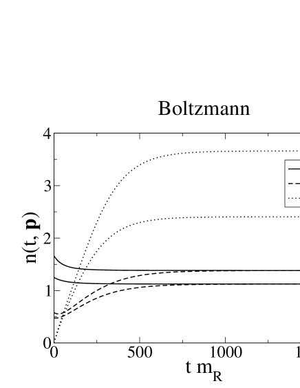
Figure 7: These plots show the time evolution of the particle number distributions for two different momentum modes and all initial conditions (cf. Fig. 6) as determined by the Boltzmann and the Kadanoff-Baym equations, respectively. We see that the Kadanoff-Baym equations respect full universality, whereas in the case of the Boltzmann equation only a restricted universality is maintained, cf. Fig. 8.

$$\omega\left(t=0,\bm{p}\right)=\sqrt{m_{R}^{2}+\bm{p}^{2}}\;.$$

Figs. 7 and 8 show the evolution of the particle number distributions for two momentum modes and the corresponding equilibrium particle number distributions, respectively, for all initial conditions. In the left plots we can see, that the Kadanoff-Baym equations lead to a universal equilibrium particle number density. The left plot in Fig. 7 shows that the particle number distributions may evolve quite differently for early times. However, respecting universality, for any given momentum mode all distributions approach the same late-time value. This plot is supplemented by the left plot in Fig. 8. There, one can see that the various particle number densities, after equilibrium has effectively been reached, indeed completely agree. Hence, this plot proves that we could have shown plots similar to the left one in Fig. 7 for all momentum modes. In particular the predicted temperature, given by the inverse slope of the line, is the same for all initial conditions. In contrast to this, the right plots reveal that the Boltzmann equation respects only a restricted universality. In general, e.g. for the initial conditions IC1 and IC3, for any given momentum mode the particle number densities will not approach the same late-time value. For both momentum modes shown in Fig. 7 a considerable discrepancy is revealed. However, for the special case of the initial conditions IC1 and IC2, which, as mentioned above, correspond to the same initial average particle number density, the late-time results do agree.

The reason for the observed restriction of universality can be extracted from Fig. 9. There we show the time evolution of the total particle number per volume

$$N_{tot}\left(t\right)=\int\frac{d^{3}p}{\left(2\pi\right)^{3}}\;n\left(t,\bm{p}\right)\;.$$

In general the Kadanoff-Baym equations conserve the average energy density and global charges baymKadanoff1961a ; Baym:1962sx ; Ivanov:1998nv .

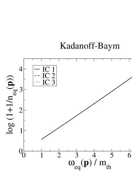
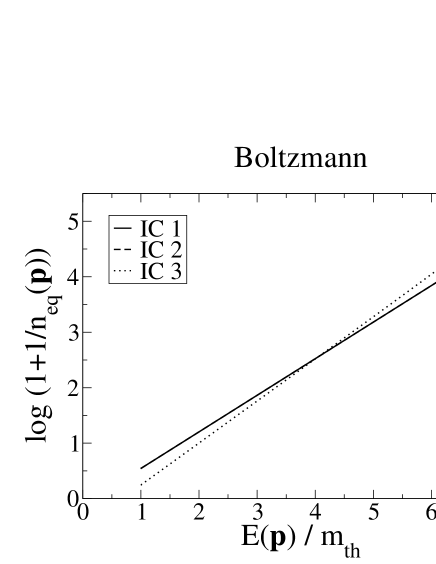
Figure 8: Here, we plotted the equilibrium particle number distributions obtained for times when thermal equilibrium has effectively been reached, against the corresponding thermal energy densities. The thermal mass is given by the zero mode of the effective kinetic equilibrium energy density as determined by the Kadanoff-Baym equations: $m_{th}=\omega_{eq}\left(\bm{p}=0\right)$. For a given initial condition, the temperature is given by the inverse slope of the line and the chemical potential is obtained from the y-axis intercept divided by $-\beta$. Supplementing Fig. 7 we observe full (restricted) universality in the case of the Kadanoff-Baym (Boltzmann) equations. In particlular, the Kadanoff-Baym equations lead to a universal temperature $T=1.68\;m_{th}$ and a universally vanishing chemical potential. In contrast to this, the Boltzmann equation gives $T=1.52\;m_{th}$ and $\mu=0.18\;m_{th}$ for the initial conditions IC1 and IC2, and $T=1.32m_{th}$ and $\mu=0.68\;m_{th}$ for IC3.

However, as there is no conserved charge in our theory, the total particle number need not be conserved. Indeed, the Kadanoff-Baym equations include off-shell particle creation and annihilation Aarts:2001qa . Consequently, the total particle number may change, and in fact approaches a universal equilibrium value. In contrast to this, due to the quasi-particle (or on-shell) approximation particle number changing processes are kinematically forbidden in the Boltzmann equation. The Boltzmann equation only includes two-particle scattering, which leaves the total particle number constant. Of course, this additional constant of motion severely restricts the evolution of the particle number density. Therefore the Boltzmann equation cannot lead to a universal quantum thermal equilibrium. Only initial conditions for which the average energy density and the total particle number agree from the very beginning, lead to the same equilibrium results.

In a system allowing for creation and annihilation of particles, the chemical potential of particles, whose total number is not restricted by any conserved quantity, must vanish in thermodynamical equilibrium. The chemical potential predicted by the Kadanoff-Baym and Boltzmann equations, respectively, is given by the y-axis intercept, extracted from Fig. 8, divided by $-\beta$. Using a ruler the reader might convince himself that the Kadanoff-Baym equations indeed lead to a universally vanishing chemical potential.

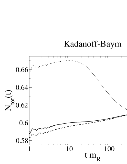
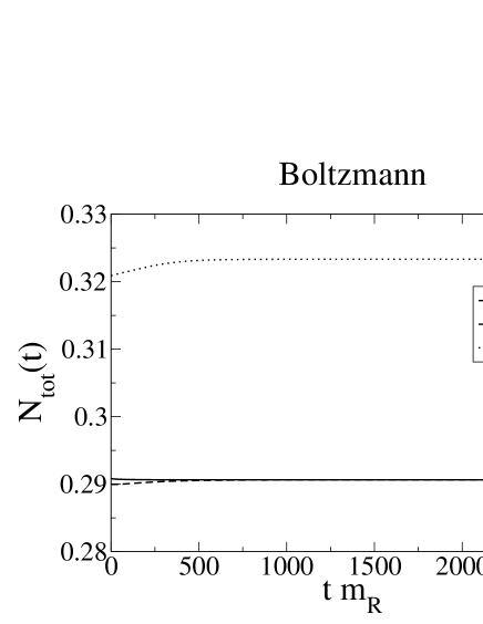
Figure 9: Time evolution of the total particle number. As expected from Ref. Aarts:2001qa , the Kadanoff-Baym equations include off-shell particle creation and annihilation. As a result the total particle number may change with time. In contrast to this the total particle number is strictly conserved in the case of the Boltzmann equation. Concerning our simulations, of course, this only holds up to numerical errors ($<0.8\%$). The quantitative disagreement of the total particle numbers in both plots can be attributed to the substantial discrepancies in the discretization schemes underlying our Boltzmann and Kadanoff-Baym numerics and are of no relevance for the purposes of the present work.

In contrast to this, even without a ruler one can see that the Boltzmann equation, in general, will lead to a non-vanishing chemical potential.

In this context, Fig. 10 exhibits further interesting results. In the upper left plot one can see that the Kadanoff-Baym equations rapidly wash out our tsunami-type initial condition IC3. In both plots on the left hand side the double-dashed-dotted lines correspond to the particle number distribution at the same time $tm_{R}=42.4$. Thus, in the lower left plot one obtains an approximate straight line already after a relatively short period of time, indicating a swift approach to kinetic equilibrium. Subsequently, this straight line is tilted until it intersects the origin of our coordinate system (full line), corresponding to a vanishing chemical potential . However, this approach to full thermodynamical (including chemical) equilibrium takes a considerably longer time Berges:2004ce . In this way, the left plots reveal two distinct time scales: a rather fast kinetic equilibration, and a very slow thermodynamical (including chemical) equilibration. These two time scales can also be identified in the left plot of Fig. 7 and in Fig. 5. The over-shooting of the particle number density for early times leads to the kinetic equilibration. In fact, the double-dashed-dotted lines correspond to the time, when the particle number distribution (equal-time propagator) reaches its maximum value in Fig. 7 (Fig. 5). Interestingly, although the initial conditions IC1 and IC2 do not show this excessive over-shooting, the corresponding particle number distributions (equal-time propagators) approach each other on the same time scale, from which on they show an almost identical evolution. The following rather long tail, again indicates that full thermalization takes place on much larger time scales.

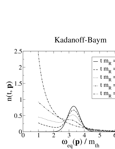
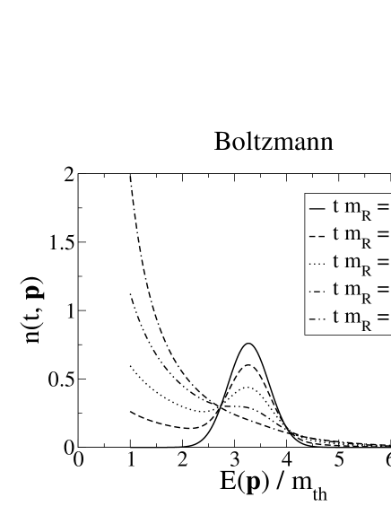
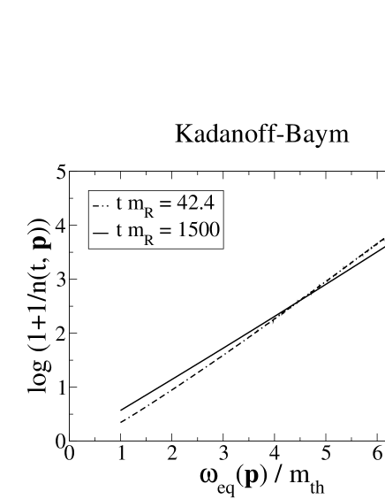
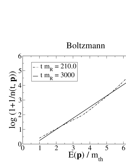
Figure 10: (Missing) separation of time scales. The particle number distribution is shown against the equilibrium energy density at various times for initial condition IC3.

The right plot in Fig. 7 shows that the steep initial evolution, which is characteristic for the Kadanoff-Baym equations, is absent in the case of the Boltzmann equation and that the Boltzmann equation leads only to a gently inclined evolution of the particle number distribution. Accordingly, the plots on the right hand side of Fig. 10 show that it takes a considerably longer time for the Boltzmann equation to reach kinetic equilibrium. As already mentioned above, in contrast to the Kadanoff-Baym equations, the Boltzmann equation cannot describe the process of chemical equilibration. Consequently, the separation of time scales furnished by the Kadanoff-Baym equations is absent in the Boltzmann case.

VII Conclusions

Starting from the 2PI effective action for a scalar $\Phi^{4}$ quantum field theory we briefly reviewed the derivation of the Kadanoff-Baym equations and the approximations which are necessary to eventually arrive at a Boltzmann equation. We solved both, the Kadanoff-Baym equations and the Boltzmann equation, numerically for spatially homogeneous and isotropic systems in 3+1 dimensions without any further approximations.

We have shown that the Kadanoff-Baym equations respect universality: For systems with equal average energy density the late time behavior coincides independent of the details of the initial conditions. In particular, independent of the initial conditions the particle number densities, temperatures and thermal masses predicted for times when equilibrium has effectively been reached coincide. The chemical potentials also coincide and vanish. Furthermore, we observed that thermalization takes place on two different time-scales: a rather fast kinetic equilibration, and a very slow thermodynamical (including chemical) equilibration.

In general Kadanoff-Baym and Boltzmann equations conserve total energy as well as global charges. In the special case of a real scalar $\Phi^{4}$ quantum field theory the quasi-particle approximation implies that the Boltzmann equation additionally conserves the total particle number. This additional constant of motion severely restricts the evolution of the system. As a result the Boltzmann equation cannot lead to a universal quantum thermal equilibrium. The Boltzmann equation respects only a restricted universality: Only initial conditions for which the average energy density and the total particle number agree from the very beginning, lead to the same equilibrium results. In particular, the Boltzmann equation cannot describe the phenomenon of chemical equilibration and, in general, will lead to a non-vanishing chemical potential. Due to the lack of chemical equilibration, the separation of time scales, which we observed for the Kadanoff-Baym equations, is absent in the case of the Boltzmann equation.

Some of the approximations that lead from the Kadanoff-Baym equations to the Boltzmann equation (namely, the gradient expansion, neglecting the Poisson brackets and the Kadanoff-Baym ansatz) are clearly motivated by equilibrium considerations. Taking the observed restriction of universality into account, we conclude that one can safely apply the Boltzmann equation only to systems which are sufficiently close to equilibrium. Accordingly, for a system far from equilibrium the results given by the Boltzmann equation should be treated with care.

In the future it will be important to perform a similar comparison between Boltzmann and Kadanoff-Baym equations for Yukawa-type quantum field theories including fermions and gauge fields. Also a treatment of Kadanoff-Baym equations on an expanding space-time should reveal interesting results. This would finally enable one to attack the problem of leptogenesis. Independent of the comparison between Boltzmann and Kadanoff-Baym equations we are looking forward to learn to which extend a full non-perturbative renormalization procedure vanHees:2001ik ; vanHees:2001pf ; vanHees:2002bv ; Blaizot:2003an ; Berges:2004hn ; Berges:2005hc affects the results quantitatively.

*

Simplifying the Boltzmann Equation

The simplification of the Boltzmann equation Dolgov:1997mb relies on the Fourier representation of the momentum conservation delta function:

$$\delta^{3}\left(\bm{m}\right)=\int\frac{d^{3}\xi}{\left(2\pi\right)^{3}}\;\exp\left(-i\bm{m}\bm{\xi}\right)\;.$$

Using spherical coordinates, we find

$$\bm{m}\bm{\xi}=m\xi\Big{(}\sin\vartheta_{m}\;\sin\vartheta_{\xi}\;\cos\left(\varphi_{m}-\varphi_{\xi}\right)+\cos\vartheta_{m}\;\cos\vartheta_{\xi}\Big{)}\;.$$

Now, we consider just the integration over the solid angle. As we integrate over the complete solid angle $\Omega_{\xi}$, it does not matter in which direction $\bm{m}$ is pointing. The result will always be the same:

$$\int d\Omega_{\xi}\exp\left(-i\bm{m}\bm{\xi}\right)=\int d\Omega_{\xi}\exp\left(-i\bm{m}_{0}\bm{\xi}\right)\;,$$

where we can choose $\bm{m}_{0}=\left(0,0,m\right)$, such that $\varphi_{m}=\vartheta_{m}=0$. Now, we can evaluate the integral quite easily:

$$\int d\Omega_{\xi}\exp\left(-i\bm{m}\bm{\xi}\right)=\int d\Omega_{\xi}\exp\left(-im\xi\cos\vartheta_{\xi}\right)=\frac{4\pi}{m\xi}\sin\left(m\xi\right)\;.$$ (20)

After we have rewritten Eq. (IV) using spherical coordinates and inserted the Fourier representation for the momentum conservation delta function, we can use Eq. (20) to perform the integrations over the solid angles. Here it is crucial first to evaluate the integrals over $\Omega_{p}$, $\Omega_{q}$ and $\Omega_{r}$, and to do the integral over $\Omega_{\xi}$ at last. We find:

$$\partial_{t}n\left(t,k\right)=\frac{\lambda^{2}}{96\pi^{4}}\int\limits_{0}^{\infty}dp\int\limits_{0}^{\infty}dq\int\limits_{0}^{\infty}dr\int\limits_{0}^{\infty}d\xi\Bigg{[}pqr\frac{\delta\left(E_{k}+E_{p}-E_{q}-E_{r}\right)}{E_{k}E_{p}E_{q}}$$

$${}\times\frac{1}{k\xi^{2}}\sin\left(k\xi\right)\;\sin\left(p\xi\right)\;\sin\left(q\xi\right)\;\sin\left(r\xi\right)$$

$${}\times\Big{(}\left(1+n_{k}\right)\left(1+n_{p}\right)n_{q}n_{r}-n_{k}n_{p}\left(1+n_{q}\right)\left(1+n_{r}\right)\Big{)}\Bigg{]}\;,$$

There are only two more steps to make in order to arrive at Eq. (IV). First, we define the auxiliary function $D\left(k,p,q,r\right)$:

$$D\left(k,p,q,r\right)=\int\limits_{0}^{\infty}d\xi\frac{1}{k\xi^{2}}\sin\left(k\xi\right)\;\sin\left(p\xi\right)\;\sin\left(q\xi\right)\;\sin\left(r\xi\right)\;.$$

This can easily be evaluated using a computer algebra program. For $k>0$ this is

$$D\left(k,p,q,r\right) = \frac{\pi}{16k}\Big{(}\left|k-p-q-r\right|-\left|k+p-q-r\right|$$

$${}-\left|k-p+q-r\right|+\left|k+p+q-r\right|$$

$${}-\left|k-p-q+r\right|+\left|k+p-q+r\right|$$

$${}+\left|k-p+q+r\right|-\left|k+p+q+r\right|\Big{)}\;,$$

and for $k=0$ we obtain

$$D\left(0,p,q,r\right) = \frac{\pi}{8}\Big{(}\mbox{sign}\left(p+q-r\right)-\mbox{sign}\left(p-q-r\right)$$

$${}+\mbox{sign}\left(p-q+r\right)-\mbox{sign}\left(p+q+r\right)\Big{)}.$$

Second, we use the energy conservation $\delta$ function to evaluate the integral over $r$, using the well-known formula

$$\delta\left(f\left(r\right)\right)=\sum_{\left\{r_{0}|f\left(r_{0}\right)=0\right\}}\frac{\delta\left(r-r_{0}\right)}{\left|\left(\frac{df}{dr}\right)_{r=r_{0}}\right|}\;.$$

$r_{0}$ is determined by the condition that the argument of the energy conservation $\delta$ function is zero:

$$E_{k}+E_{p}-E_{q}-E_{r_{0}}=0\;.$$ (21)

If this condition can be satisfied, $r_{0}$ is given by

$$r_{0}=r_{0}\left(t,k,p,q\right)=\sqrt{\left(E_{k}+E_{p}-E_{q}\right)^{2}-M^{2}\left(t\right)}\;.$$

If $k$, $p$ and $q$ are such that condition (21) cannot be satisfied, the above square root yields a purely imaginary result and $r_{0}^{2}<0$. Due to the $\Theta$ function the corresponding term does not contribute to the collision integral. After these final steps we end up exactly with Eq. (IV).

References

- (1) M. Fukugita and T. Yanagida, Baryogenesis without Grand Unification, Phys. Lett. B174 (1986) 45.
- (2) W. Buchmüller, P. Di Bari, and M. Plümacher, Leptogenesis for pedestrians, Ann. Phys. 315 (2005) 305, eprint hep-ph/0401240.
- (3) Wilfried Buchmüller and Stefan Fredenhagen, Quantum mechanics of baryogenesis, Phys. Lett. B483 (2000) 217, eprint hep-ph/0004145.
- (4) A. D. Sakharov, Violation of CP Invariance, C Asymmetry, and Baryon Asymmetry of the Universe, JETP Lett. 5 (1967) 24.
- (5) I. Arsene et al. (BRAHMS), Quark gluon plasma and color glass condensate at RHIC? The perspective from the BRAHMS experiment, Nucl. Phys. A757 (2005) 1, eprint nucl-ex/0410020.
- (6) B. B. Back et al. (PHOBOS), The PHOBOS perspective on discoveries at RHIC, Nucl. Phys. A757 (2005) 28, eprint nucl-ex/0410022.
- (7) J. Adams et al. (STAR), Experimental and theoretical challenges in the search for the quark gluon plasma: The STAR collaboration’s critical assessment of the evidence from RHIC collisions, Nucl. Phys. A757 (2005) 102, eprint nucl-ex/0501009.
- (8) K. Adcox et al. (PHENIX), Formation of dense partonic matter in relativistic nucleus nucleus collisions at RHIC: Experimental evaluation by the PHENIX collaboration, Nucl. Phys. A757 (2005) 184, eprint nucl-ex/0410003.
- (9) J. Berges, S. Borsányi, and C. Wetterich, Prethermalization, Phys. Rev. Lett. 93 (2004) 142002, eprint hep-ph/0403234.
- (10) A. H. Mueller and D. T. Son, On the equivalence between the Boltzmann equation and classical field theory at large occupation numbers, Phys. Lett. B582 (2004) 279, eprint hep-ph/0212198.
- (11) Sangyong Jeon, The Boltzmann equation in classical and quantum field theory, Phys. Rev. C72 (2005) 014907, eprint hep-ph/0412121.
- (12) Gordon Baym and Leo P. Kadanoff, Quantum Statistical Mechanics (Benjamin, New York, 1962)
- (13) P. Danielewicz, Quantum Theory of Nonequilibrium Processes I, Annals Phys. 152 (1984) 239.
- (14) Yu. B. Ivanov, J. Knoll, and D. N. Voskresensky, Resonance Transport and Kinetic Entropy, Nucl. Phys. A672 (2000) 313, eprint nucl-th/9905028.
- (15) J. Knoll, Yu. B. Ivanov, and D. N. Voskresensky, Exact Conservation Laws of the Gradient Expanded Kadanoff- Baym Equations, Annals Phys. 293 (2001) 126, eprint nucl-th/0102044.
- (16) Jean-Paul Blaizot and Edmond Iancu, The quark-gluon plasma: Collective dynamics and hard thermal loops, Phys. Rept. 359 (2002) 355, eprint hep-ph/0101103.
- (17) Jürgen Berges, Controlled nonperturbative dynamics of quantum fields out of equilibrium, Nucl. Phys. A699 (2002) 847, eprint hep-ph/0105311.
- (18) Gert Aarts and Jürgen Berges, Nonequilibrium time evolution of the spectral function in quantum field theory, Phys. Rev. D64 (2001) 105010, eprint hep-ph/0103049.
- (19) Edward W. Kolb and Stephen Wolfram, Baryon Number Generation in the Early Universe, Nucl. Phys. B172 (1980) 224.
- (20) Edward W. Kolb and Michael S. Turner, The Early Universe (Addison-Wesley, 1990)
- (21) H. S. Köhler, Memory and correlation effects in nuclear collisions, Phys. Rev. C51 (1995) 3232
- (22) K. Morawetz and H. S. Köhler, Formation of correlations and energy-conservation at short time scales, Eur. Phys. J. A4 (1999) 291, eprint nucl-th/9802082.
- (23) S. Juchem, W. Cassing, and C. Greiner, Quantum dynamics and thermalization for out-of-equilibrium -theory, Phys. Rev. D69 (2004) 025006, eprint hep-ph/0307353.
- (24) Gordon Baym and Leo P. Kadanoff, Conservation Laws and Correlation Functions, Phys. Rev. 124 (1961) 287
- (25) Gordon Baym, Selfconsistent approximation in many body systems, Phys. Rev. 127 (1962) 1391.
- (26) Yu. B. Ivanov, J. Knoll, and D. N. Voskresensky, Self-consistent approximations to non-equilibrium many-body theory, Nucl. Phys. A657 (1999) 413, eprint hep-ph/9807351.
- (27) R. Jackiw, Functional evaluation of the effective potential, Phys. Rev. D9 (1974) 1686.
- (28) John M. Cornwall, R. Jackiw, and E. Tomboulis, Effective Action for Composite Operators, Phys. Rev. D10 (1974) 2428.
- (29) E. Calzetta and B. L. Hu, Nonequilibrium quantum fields: Closed-time-path effective action, Wigner function and Boltzmann equation, Phys. Rev. D37 (1988) 2878.
- (30) Jürgen Berges and Jürgen Cox, Thermalization of quantum fields from time-reversal invariant evolution equations, Phys. Lett. B517 (2001) 369, eprint hep-ph/0006160.
- (31) Jürgen Berges, Szabolcs Borsányi, and Julien Serreau, Thermalization of fermionic quantum fields, Nucl. Phys. B660 (2003) 51, eprint hep-ph/0212404.
- (32) Gert Aarts and Jürgen Berges, Classical aspects of quantum fields far from equilibrium, Phys. Rev. Lett. 88 (2002) 041603, eprint hep-ph/0107129.
- (33) Gert Aarts and Jose M. Martínez Resco, Transport coefficients from the 2PI effective action, Phys. Rev. D68 (2003) 085009, eprint hep-ph/0303216.
- (34) J. Berges, Sz. Borsányi, U. Reinosa, and J. Serreau, Renormalized thermodynamics from the 2PI effective action, Phys. Rev. D71 (2005) 105004, eprint hep-ph/0409123.
- (35) Julian S. Schwinger, Brownian motion of a quantum oscillator, J. Math. Phys. 2 (1961) 407.
- (36) Pradip M. Bakshi and Kalyana T. Mahanthappa, Expectation value formalism in quantum field theory. 1, J. Math. Phys. 4 (1963) 1.
- (37) Pradip M. Bakshi and Kalyana T. Mahanthappa, Expectation value formalism in quantum field theory. 2, J. Math. Phys. 4 (1963) 12.
- (38) L. V. Keldysh, Diagram technique for nonequilibrium processes, Sov. Phys. JETP 20 (1965) 1018.
- (39) Jürgen Berges and Markus M. Müller, Nonequilibrium quantum fields with large fluctuations, in Progress in Nonequilibrium Green’s Functions 2 (edited by M. Bonitz and D. Semkat, World Scientific Publ., Singapore, 2003), 367, eprint hep-ph/0209026
- (40) S. Juchem, W. Cassing, and C. Greiner, Nonequilibrium quantum-field dynamics and off-shell transport for -theory in 2+1 dimensions, Nucl. Phys. A743 (2004) 92, eprint nucl-th/0401046.
- (41) Jürgen Berges and Szabolcs Borsányi, Nonequilibrium quantum fields from first principles (2005), eprint hep-th/0512010.
- (42) Jürgen Berges and Szabolcs Borsányi, Range of validity of transport equations (2005), eprint hep-ph/0512155.
- (43) Jürgen Berges, Szabolcs Borsányi, and Christof Wetterich, Isotropization far from equilibrium (2005), eprint hep-ph/0505182.
- (44) A. D. Dolgov, S. H. Hansen, and D. V. Semikoz, Non-equilibrium corrections to the spectra of massless neutrinos in the early universe, Nucl. Phys. B503 (1997) 426, eprint hep-ph/9703315.
- (45) Jürgen Berges, Introduction to nonequilibrium quantum field theory, AIP Conf. Proc. 739 (2005) 3, eprint hep-ph/0409233.
- (46) István Montvay and Gernot Münster, Quantum fields on a lattice (Cambridge University Press, 1994)
- (47) Matteo Frigo and Steven G. Johnson, FFTW Reference Manual (Version 3.1, 2006)
- (48) Alejandro Arrizabalaga, Jan Smit, and Anders Tranberg, Equilibration in theory in 3+1 dimensions, Phys. Rev. D72 (2005) 025014, eprint hep-ph/0503287.
- (49) Mark Galassi et al., GNU Scientific Library Reference Manual (Version 1.5, 2004). See also pressEtAl1988a .
- (50) Hendrik van Hees and Jörn Knoll, Renormalization in self-consistent approximations schemes at finite temperature. I: Theory, Phys. Rev. D65 (2002) 025010, eprint hep-ph/0107200.
- (51) Hendrik van Hees and Jörn Knoll, Renormalization of self-consistent approximation schemes. II: Applications to the sunset diagram, Phys. Rev. D65 (2002) 105005, eprint hep-ph/0111193.
- (52) Hendrik van Hees and Jörn Knoll, Renormalization in self-consistent approximation schemes at finite temperature. III: Global symmetries, Phys. Rev. D66 (2002) 025028, eprint hep-ph/0203008.
- (53) Jean-Paul Blaizot, Edmond Iancu, and Urko Reinosa, Renormalization of phi-derivable approximations in scalar field theories, Nucl. Phys. A736 (2004) 149, eprint hep-ph/0312085.
- (54) Jürgen Berges, Szabolcs Borsányi, Urko Reinosa, and Julien Serreau, Nonperturbative renormalization for 2PI effective action techniques, Annals Phys. 320 (2005) 344, eprint hep-ph/0503240.
- (55) William H. Press et al., Numerical Recipes in C (Cambridge University Press, 1988)