TUM-HEP–614/05
hep–ph/0512143
Improved Limit on $\theta_{13}$ and Implications for Neutrino Masses in Neutrino-less Double Beta Decay and Cosmology
 

We analyze the impact of a measurement, or of an improved bound, on $\theta_{13}$ for the determination of the effective neutrino mass in neutrino-less double beta decay and cosmology. In particular, we discuss how an improved limit on (or a specific value of) $\theta_{13}$ can influence the determination of the neutrino mass spectrum via neutrino-less double beta decay. We also discuss the interplay with improved cosmological neutrino mass searches.

1 Introduction

The absolute mass scale and the Majorana nature of neutrinos are among the central topics of the future research program in neutrino physics [1, 2]. In addition, the value of the currently unknown mixing matrix element $|U_{e3}|=\sin\theta_{13}$ is of central importance, since it is a strong discriminator for neutrino mass models. The magnitude of $|U_{e3}|$ is also important for future efforts to probe leptonic $CP$ violation and/or the mass ordering in oscillation experiments (see e.g. [3]). Neutrino-less double beta decay (0$\nu\beta\beta$) is the best known method to address both the Majorana nature of neutrinos, as well as the absolute mass scale. Several ongoing and planned experiments, such as NEMO3 [4], CUORICINO [5], CUORE [6], MAJORANA [7], GERDA [8], EXO [9], MOON [10], COBRA [11], XMASS, DCBA [12], CANDLES [13], CAMEO [14] aim at observing the process

$$(A,Z)\rightarrow(A,Z+2)+2\,e^{-}~{}.$$

If mediated by light Majorana neutrinos, the square root of the decay width of 0$\nu\beta\beta$ is proportional to a so-called effective mass which is given by the following coherent sum:

$$\mbox{$\left|m_{ee}\right|$}\equiv\left|\sum_{i}m_{i}\,U_{ei}^{2}\right|~{},$$ (1)

where $m_{i}$ is the mass of the $i^{th}$ neutrino mass state and where the sum is over all light neutrino mass states. $U_{ei}$ are the elements of the leptonic mixing matrix [15] which we parameterize here as

$$U=\left(\begin{array}[]{ccc}c_{12}c_{13}&s_{12}c_{13}&s_{13}\,e^{-i\delta}\\[5.69046pt] -s_{12}c_{23}-c_{12}s_{23}s_{13}e^{i\delta}&c_{12}c_{23}-s_{12}s_{23}s_{13}e^{i\delta}&s_{23}c_{13}\\[5.69046pt] s_{12}s_{23}-c_{12}c_{23}s_{13}e^{i\delta}&-c_{12}s_{23}-s_{12}c_{23}s_{13}e^{i\delta}&c_{23}c_{13}\\ \end{array}\right){\rm diag}(1,e^{i\alpha},e^{i\beta})\,,$$ (5)

where we have used the usual notations $c_{ij}=\cos\theta_{ij}$, $s_{ij}=\sin\theta_{ij}$. $\delta$ is the Dirac $CP$-violation phase, $\alpha$ and $\beta$ are the two Majorana $CP$-violation phases [16]. The best current limit on the effective mass is given by the Heidelberg-Moscow collaboration [17]

$$\mbox{$\left|m_{ee}\right|$}\leq 0.35\,\zeta~{}{\rm eV}~{},$$ (6)

where $\zeta={\cal O}(1)$ indicates an uncertainty due to uncertainties in the calculation of the nuclear matrix elements of 0$\nu\beta\beta$. Similar results were obtained by the IGEX collaboration [18]. The above mentioned experiments will improve the current bound by one order of magnitude. In terms of the neutrino mass matrix,

$$m_{\alpha\beta}=U_{\alpha i}\,m_{i}\,\delta_{ij}\,U^{T}_{j\beta}~{},$$ (7)

$\left|m_{ee}\right|$ is nothing but the $ee$ element in the basis where the charged lepton mass matrix is real and diagonal. Neutrino-less double beta decay therefore probes directly an element of the mass matrix, which is a unique feature, not possible in the quark sector. $\left|m_{ee}\right|$ in Eq. (1) depends on the oscillation parameters, the Majorana phases and the overall neutrino mass scale. This means that $\left|m_{ee}\right|$ depends on 7 out of 9 parameters contained in the neutrino mass matrix. It depends also on the neutrino mass ordering, which can be normal or inverted. It is interesting that the effective mass is a function of all unknowns of neutrino physics except for the Dirac phase and $\theta_{23}$. The effective mass is therefore a probe of the neutrino mass scale and interestingly also of $\theta_{13}$. We focus in this work on the dependence on $\theta_{13}$, where significant improvements are expected. The current limit $\sin^{2}2\theta_{13}<0.2$ will be somewhat improved by the on-going or up-coming neutrino beam experiments MINOS [20] and ICARUS [21] as well as OPERA [22], respectively. Further significant improvement by one order of magnitude compared to the existing bound will come within about 5 years from reactor experiments such as Double Chooz [23]. A few years later, the next generation of superbeam experiments, T2K [24] and No$\nu$A [25], will further improve the measurements or the bound of $\theta_{13}$. The absolute neutrino mass scale will also be attacked by improved measurements of the end-point spectrum of tritium decay [26]. Furthermore, improved cosmological measurements will improve our knowledge on the absolute neutrino mass scale from the role of neutrinos as hot dark matter in the cosmological structure formation [27]. Altogether one can safely expect that the current limits will improve at least by one order of magnitude.

It is therefore interesting to analyze the interplay of $\theta_{13}$ with the neutrino mass scale, the neutrino mass ordering and 0$\nu\beta\beta$. In Section 2 we discuss the general dependence of the effective mass as a function of the neutrino observables. In Section 3 we discuss then in detail the case of normal mass ordering. We show that a very stringent limit on the effective mass leads to a limited range of values of the smallest neutrino mass, which translates into a certain range of the sum of neutrino masses as measurable in cosmology. The dependence on $\theta_{13}$ of these values is stressed. Section 4 deals then with the inverted mass ordering, and in Section 5 we discuss how $\theta_{13}$ influences the possibility to distinguish between normal and inverted mass ordering via 0$\nu\beta\beta$. The uncertainty stemming from the nuclear matrix element calculations is also taken into account. Finally, we conclude in Section 6.

2 Properties of the Effective Mass: General Aspects

In this and the next two Sections we will discuss in some detail the value of the effective mass in terms of the known and unknown neutrino parameters [28, 29, 30, 31], for a recent review see [32].

The effective mass is the absolute value of the mass matrix element $m_{ee}$, i.e., for three flavors it is a sum of three terms

$$\left|m_{ee}\right|\equiv\left|\sum U_{ei}^{2}\,m_{i}\right|\mbox{ with }m_{ee}=|m_{ee}^{(1)}|+|m_{ee}^{(2)}|\,e^{2i\alpha}+|m_{ee}^{(3)}|\,e^{2i\beta}~{},$$ (8)

which is visualized in Fig. 1 as the sum of three complex vectors $m_{ee}^{(1,2,3)}$. The Majorana phases $2\alpha$ and $2\beta$ correspond then to the relative orientation of the three vectors.

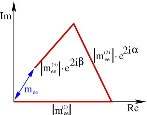
Figure 1: The mass matrix element $m_{ee}$ as a sum of three complex vectors.

In terms of the neutrino masses and mixing angles, we have

$$|m_{ee}^{(1)}| = m_{1}\,|U_{e1}|^{2}=m_{1}\,c_{12}^{2}\,c_{13}^{2}~{},$$

$$|m_{ee}^{(2)}| = m_{2}\,|U_{e2}|^{2}=m_{2}\,s_{12}^{2}\,c_{13}^{2}~{},$$ (9)

$$|m_{ee}^{(3)}| = m_{3}\,|U_{e3}|^{2}=m_{3}\,s_{13}^{2}~{}.$$

Normal mass ordering corresponds to $m_{3}>m_{2}>m_{1}$, whereas for an inverted ordering we have $m_{2}>m_{1}>m_{3}$. The effective mass to be extracted from neutrino-less double beta decay depends crucially on the neutrino mass spectrum. Fixing for the solar neutrino sector $\mbox{$\Delta m^{2}_{\odot}$}=m_{2}^{2}-m_{1}^{2}>0$, we have for the atmospheric neutrino sector either $m_{3}^{2}-m_{1}^{2}>0$ (normal ordering) or $m_{3}^{2}-m_{1}^{2}<0$ (inverted ordering). We use a notation where $\mbox{$\Delta m^{2}_{\rm A}$}\equiv|m_{3}^{2}-m_{1}^{2}|$ is always positive. The best-fit values and the $1\sigma$ and $3\sigma$ ranges of the oscillation parameters which will be used in this work are [33]

$$\Delta m^{2}_{\odot} = 7.9^{+0.3\,,\,1.0}_{-0.3\,,\,0.8}\cdot 10^{-5}\mbox{ eV}^{2}~{},$$

$$\sin^{2}\theta_{12} = 0.31^{+0.02\,,\,0.09}_{-0.03\,,\,0.07}~{},$$

$$\Delta m^{2}_{\rm A} = 2.2^{+0.37\,,\,1.1}_{-0.27\,,\,0.8}\cdot 10^{-3}\mbox{ eV}^{2}~{},$$ (10)

$$\sin^{2}\theta_{23} = 0.50^{+0.06\,,\,0.18}_{-0.05\,,\,0.16}~{},$$

$$\sin^{2}\theta_{13} < 0.012~{}(0.046)~{}.$$

The best-fit value for $\sin^{2}\theta_{13}$ is 0. The two larger masses for each ordering are given in terms of the smallest mass and the mass squared differences as

$$\begin{array}[]{ccc}\text{normal:}&m_{2}=\sqrt{m_{1}^{2}+\mbox{$\Delta m^{2}_{\odot}$}}~{};~{}~{}~{}~{}~{}~{}~{}~{}~{}~{}~{}~{}~{}~{}~{}m_{3}=\sqrt{m_{1}^{2}+\mbox{$\Delta m^{2}_{\rm A}$}}~{},\\ \text{inverted:}&m_{2}=\sqrt{m_{3}^{2}+\mbox{$\Delta m^{2}_{\odot}$}+\mbox{$\Delta m^{2}_{\rm A}$}}~{};~{}~{}~{}~{}m_{1}=\sqrt{m_{3}^{2}+\mbox{$\Delta m^{2}_{\rm A}$}}~{}.\end{array}$$ (13)

Of special interest are the following three extreme cases:

normal hierarchy (NH): $$~{}~{}~{}~{}~{}~{}~{}~{}~{}~{}~{}~{}~{}|m_{3}|\simeq\sqrt{\mbox{$\Delta m^{2}_{\rm A}$}}\gg|m_{2}|\simeq\sqrt{\mbox{$\Delta m^{2}_{\odot}$}}\gg|m_{1}|~{},$$ (14)

inverted hierarchy (IH): $$|m_{2}|\simeq|m_{1}|\simeq\sqrt{\mbox{$\Delta m^{2}_{\rm A}$}}\gg|m_{3}|~{},$$ (15)

quasi-degeneracy (QD): $$~{}~{}~{}~{}~{}~{}~{}~{}m_{0}\equiv|m_{1}|\simeq|m_{2}|\simeq|m_{3}|\gg\sqrt{\mbox{$\Delta m^{2}_{\rm A}$}}~{}.$$ (16)

The order of magnitude of the effective mass in those spectra is $\sqrt{\mbox{$\Delta m^{2}_{\odot}$}},\sqrt{\mbox{$\Delta m^{2}_{\rm A}$}}$ and $m_{0}$, respectively (for recent analyzes of the effective mass in terms of the neutrino mass spectrum, see [30, 31]). Within our parameterization Eq. (5), it is sufficient to vary the Majorana phases $\alpha$ and $\beta$ between 0 and $\pi$ in order to obtain the full physical range of $\left|m_{ee}\right|$. If there were processes sensitive to the off-diagonal elements of the neutrino mass matrix (from all that we know, there are not [34]), then one would have to vary the phases in their full range between 0 and $2\pi$ to obtain the full physical range.

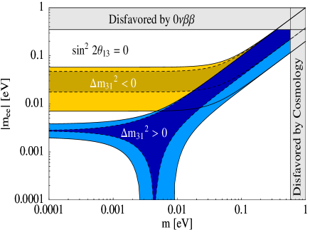
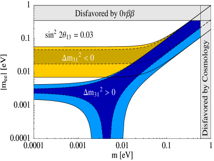
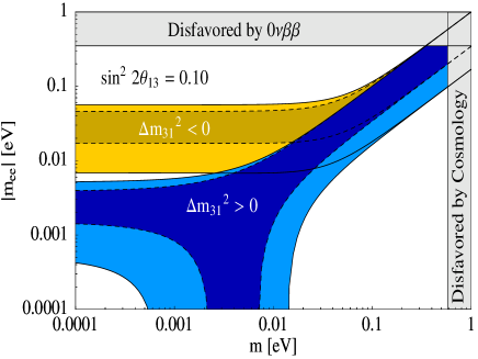
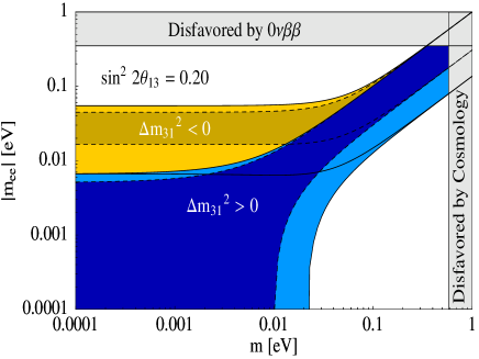
Figure 2: The effective mass (in eV) for the normal and inverted ordering as a function of the smallest neutrino mass (in eV) for different values of $\sin^{2}2\theta_{13}$. The prediction for the best-fit values of the oscillation parameters and for the $3\sigma$ ranges is given. A typical bound from cosmology and the limit on the effective mass from Eq. (6) are indicated.

An interesting aspect is the minimal or maximal value of the effective mass. Therefore it is helpful to consider the respective ranges of the three terms $|m_{ee}^{(1,2,3)}|$. Maximal $\left|m_{ee}\right|$ is obtained when all three $|m_{ee}^{(i)}|$ add up, or, in the geometrical picture of Fig. 1, when all three vectors $m_{ee}^{(1,2,3)}$ point in the same direction. To find the minimal value of $\left|m_{ee}\right|$, one has to identify the dominating $|m_{ee}^{(i)}|$. In case of $|m_{ee}^{(i)}|>|m_{ee}^{(j)}|+|m_{ee}^{(k)}|$, the minimal effective mass $\mbox{$\left|m_{ee}\right|$}_{\rm min}$ is obtained by subtracting the two smaller terms from the dominating one. Simply adding or subtracting all three terms is equivalent to trivial values of the Majorana phases of 0 or $\pi/2$, which corresponds to the conservation of $CP$ [35]. Hence, both the minimal and maximal $\left|m_{ee}\right|$ occur in a $CP$ conserving situation. Note, however, that the Dirac phase which is measurable in oscillation experiments can still be non-zero. We introduce the notation $--$ to label the case when the second and third term are subtracted from the first one. Analogously, the notation for the other two cases is $-+$ and $+-$. In Table 1 we summarize the three possibilities.

Scenario	Majorana phases	$\left|m_{ee}\right|_{\rm min}$
$\begin{array}[]{c}\mbox{\small first term dominates}\\ --\end{array}$	$\alpha=\beta=\frac{\pi}{2}$	$\left|m_{1}c_{12}^{2}c_{13}^{2}-\sqrt{m_{1}^{2}+\mbox{$\Delta m^{2}_{\odot}$}}s_{12}^{2}c_{13}^{2}-\sqrt{m_{1}^{2}+\mbox{$\Delta m^{2}_{\rm A}$}}s_{13}^{2}\right|$
$\begin{array}[]{c}\mbox{\small second term dominates}\\ -+\end{array}$	$\alpha=\frac{\pi}{2},\ \beta=0$	$\left|m_{1}c_{12}^{2}c_{13}^{2}-\sqrt{m_{1}^{2}+\mbox{$\Delta m^{2}_{\odot}$}}s_{12}^{2}c_{13}^{2}+\sqrt{m_{1}^{2}+\mbox{$\Delta m^{2}_{\rm A}$}}s_{13}^{2}\right|$
$\begin{array}[]{c}\mbox{\small third term dominates}\\ +-\end{array}$	$\alpha=0,\ \beta=\frac{\pi}{2}$	$\left|m_{1}c_{12}^{2}c_{13}^{2}+\sqrt{m_{1}^{2}+\mbox{$\Delta m^{2}_{\odot}$}}s_{12}^{2}c_{13}^{2}-\sqrt{m_{1}^{2}+\mbox{$\Delta m^{2}_{\rm A}$}}s_{13}^{2}\right|$

Table 1: Minimal values of $\left|m_{ee}\right|$ for dominance of one of the $|m_{ee}^{(i)}|$.

Figure 3: The main properties of the effective mass as function of the smallest neutrino mass. We indicated the relevant formulae and the three important regimes: hierarchical, cancellation (only possible for normal mass ordering) and quasi-degeneracy. The value of $\sin^{2}2\theta_{13}=0.02$ has been chosen, we defined $t_{12}^{2}=\tan^{2}\theta_{12}$ and $m_{0}$ is the common mass scale (measurable in KATRIN or by cosmology via $\Sigma/3$) for quasi-degenerate neutrino masses $m_{1}\simeq m_{2}\simeq m_{3}\equiv m_{0}$.

Using the best-fit and 3$\sigma$ oscillation parameters from Ref. [33], we can now plot the effective mass as a function of the smallest neutrino mass. This is shown in Fig. 2, where we assumed different representative values of $\theta_{13}$, corresponding to $\sin^{2}2\theta_{13}=0$, 0.03, 0.1 and 0.2. A typical bound on the sum of neutrino masses $\Sigma\equiv\sum m_{i}$ of 1.74 eV is also included (hence $m<0.58$ eV for the lightest neutrino mass), obtained by an analysis of SDSS and WMAP data [36]. Moreover, we indicated the limit on the effective mass from Eq. (6), where the horizontal line corresponds to $\zeta=1$, i.e., everything above the line is unlikely. Among the oscillation parameters crucial for 0$\nu\beta\beta$, the atmospheric $\Delta m^{2}$ will be known with some precision in the medium future [3]. Generating plots like Fig. 2 with an assumed error on $\Delta m^{2}_{\rm A}$ of 10 % will reveal that the maximal effective mass for the inverted ordering is slightly smaller and that the minimal effective mass for the normal ordering is slightly larger. For our purposes, this will not change the outcome of our conclusions.

Several features of the figures are immediately identified:

• the effective mass for the normal mass ordering can become very small or even vanish for certain small values of $m_{1}$. The range of such values of $m_{1}$ (“the chimney”) becomes larger with increasing $\sin^{2}2\theta_{13}$;

• in case of a normal ordering and a small value of $m_{1}$, the minimal value of the effective mass decreases with increasing $\sin^{2}2\theta_{13}$;

• for small neutrino mass values there is a gap between the effective mass in case of a normal and inverted ordering. The size of this gap shrinks with increasing $\sin^{2}2\theta_{13}$.

We conclude that there is some interesting interplay between the value of $\theta_{13}$ and the effective mass as measurable in 0$\nu\beta\beta$. In the following, we shall perform a detailed analysis of the effective mass for both mass orderings in order to analytically understand in particular the features 1.) and 2.) from above. Then we focus on issue 3.) and analyze the gap between the minimal value of $\left|m_{ee}\right|$ for the inverted ordering and the maximal value of $\left|m_{ee}\right|$ for the normal ordering. In Figure 3 we show the outcome of the coming analysis, taking a typical value of $\sin^{2}2\theta_{13}=0.02$. We indicate the relevant regimes and explicitely include the formulae which describe the minimal and maximal values of $\left|m_{ee}\right|$ in certain ranges.

3 The Effective Mass for the Normal Mass Ordering

Let us begin with the normal mass ordering. The effective mass is the absolute value of

$$m_{ee}^{\rm nor}=m_{1}\,c_{12}^{2}\,c_{13}^{2}+\sqrt{m_{1}^{2}+\mbox{$\Delta m^{2}_{\odot}$}}\,s_{12}^{2}\,c_{13}^{2}\,e^{2i\alpha}+\sqrt{m_{1}^{2}+\mbox{$\Delta m^{2}_{\rm A}$}}\,s_{13}^{2}\,e^{2i\beta}~{}.$$ (17)

The maximum of the effective mass is obtained when the Majorana phases are given by $\alpha=\beta=0$. The effective mass is then directly given by the real $m_{ee}$:

$$\mbox{$\left|m_{ee}\right|$}^{\rm nor}_{\rm max}=m_{1}\,c_{12}^{2}\,c_{13}^{2}+\sqrt{m_{1}^{2}+\mbox{$\Delta m^{2}_{\odot}$}}\,s_{12}^{2}\,c_{13}^{2}+\sqrt{m_{1}^{2}+\mbox{$\Delta m^{2}_{\rm A}$}}\,s_{13}^{2}~{}.$$ (18)

Obviously, the largest value of the effective mass is obtained when all involved parameters, $\Delta m^{2}_{\odot}$, $\Delta m^{2}_{\rm A}$, $\theta_{13}$ and $s_{12}^{2}$ take their maximally allowed values. For the best-fit, 1 and 3$\sigma$ values of the oscillation parameters, the predictions are $\mbox{$\left|m_{ee}\right|$}^{\rm nor}_{\rm max}=0.10,(0.10,0.10)\mbox{ eV}$ when $m_{1}=0.1$ eV, $\mbox{$\left|m_{ee}\right|$}^{\rm nor}_{\rm max}=0.011,(0.012,0.014)\mbox{ eV}$ when $m_{1}=0.01$ eV, and $\mbox{$\left|m_{ee}\right|$}^{\rm nor}_{\rm max}=0.0066,(0.0073,0.0096)\mbox{ eV}$ for $m_{1}=0.005$ eV.

On the other hand, an analytic expression for the minimal value of the effective mass is not found easily in every case. Only for very small and rather large values of the smallest neutrino mass one can always identify the dominating $|m_{ee}^{(i)}|$. A more complicated situation occurs for values of $\left|m_{ee}\right|$ below roughly $10^{-3}$ eV, i.e., when the effective mass is practically zero. This interesting region of the plots in Fig. 2 will be dealt with in detail in Section 3.2. In this case typically two or all three $|m_{ee}^{(i)}|$ are of very similar magnitude and small offsets in the oscillation parameters or $m_{1}$ can change the relative ordering of the $|m_{ee}^{(i)}|$. Some examples for the ranges of the $|m_{ee}^{(i)}|$ are given in Table 2 and 3, inserting the 1 and 3$\sigma$ oscillation parameters. If one of the three $|m_{ee}^{(i)}|$ dominates, we indicated this by writing its value in bold face.

$m_{1}$ [eV]	$\sin^{2}2\theta_{13}$	$|m_{ee}^{(1)}|$ [eV]	$|m_{ee}^{(2)}|$ [eV]	$|m_{ee}^{(3)}|$ [eV]
0.1	0	0.067–0.072	0.028–0.033	0.0000
	0.05	0.066–0.071	0.028–0.033	0.0014
	0.2	0.063–0.068	0.027–0.031	0.0058–0.0059
0.01	0	0.0067–0.0072	0.0037–0.0045	0.0000
	0.05	0.0066–0.0071	0.0037–0.0044	(5.7–6.5)$\cdot 10^{-4}$
	0.2	0.0063–0.0068	0.0035–0.0042	0.0024–0.0027
0.001	0	(6.7–7.2)$\cdot 10^{-4}$	0.0025–0.0030	0.000
	0.05	(6.6–7.1)$\cdot 10^{-4}$	0.0024–0.0030	(5.6–6.4)$\cdot 10^{-4}$
	0.2	(6.3–6.8)$\cdot 10^{-4}$	0.0023–0.0028	0.0023–0.0027
0.0001	0	(6.7–7.2)$\cdot 10^{-5}$	0.0024–0.0030	0.0000
	0.05	(6.6–7.1)$\cdot 10^{-5}$	0.0024–0.0030	(5.6–6.4)$\cdot 10^{-4}$
	0.2	(6.3–6.8)$\cdot 10^{-5}$	0.0023–0.0028	0.0023–0.0027

Table 2: 1$\sigma$ ranges of $|m_{ee}^{(i)}|$ for different values of $m_{1}$ and $\theta_{13}$. Bold faced terms indicate dominance of the respective term over the whole parameter range.

$m_{1}$ [eV]	$\sin^{2}2\theta_{13}$	$|m_{ee}^{(1)}|$ [eV]	$|m_{ee}^{(2)}|$ [eV]	$|m_{ee}^{(3)}|$ [eV]
0.1	0	0.060–0.076	0.024–0.040	0.0000
	0.05	0.059–0.075	0.024–0.040	0.0014–0.0015
	0.2	0.057–0.072	0.023–0.038	0.0056–0.0061
0.01	0	0.0060–0.0076	0.0031–0.0055	0.0000
	0.05	0.0059–0.0076	0.0031–0.0054	(4.9–7.4)$\cdot 10^{-4}$
	0.2	0.0057–0.0072	0.0030–0.0052	0.0020–0.0031
0.001	0	(6.0–7.6)$\cdot 10^{-4}$	0.0020–0.0038	0.000
	0.05	(5.9–7.5)$\cdot 10^{-4}$	0.0020–0.0037	(4.7-7.3)$\cdot 10^{-4}$
	0.2	(5.7–7.2)$\cdot 10^{-4}$	0.0019–0.0036	0.0020–0.0030
0.0001	0	(6.0–7.6)$\cdot 10^{-5}$	0.0020–0.0038	0.0000
	0.05	(5.9–7.5)$\cdot 10^{-5}$	0.0020–0.0037	(4.7–7.3)$\cdot 10^{-5}$
	0.2	(5.7–7.2)$\cdot 10^{-5}$	0.0019–0.0036	0.0020–0.0030

Table 3: Same as previous Table for the $3\sigma$ ranges of the oscillation parameters.

With the $1\sigma$ values used in Table 2, it turns out that for very small values of $m_{1}\mathrel{\hbox to0.0pt{\raise 2.20013pt\hbox{$<$}\hss}{\lower 2.20013pt\hbox{$\sim$}}}0.001$ eV and $\sin^{2}2\theta_{13}\mathrel{\hbox to0.0pt{\raise 2.20013pt\hbox{$<$}\hss}{\lower 2.20013pt\hbox{$\sim$}}}0.1$ the term $|m_{ee}^{(2)}|$ always dominates. For larger values of $m_{1}\mathrel{\hbox to0.0pt{\raise 2.20013pt\hbox{$>$}\hss}{\lower 2.20013pt\hbox{$\sim$}}}0.01$ eV, the term $|m_{ee}^{(1)}|$ dominates, irrespective of $\sin^{2}2\theta_{13}$. These conclusions are rather unaffected by the use of 1 or 3$\sigma$ ranges, as can be seen by comparing Tables 2 and 3.

3.1 The strictly hierarchical part: $m_{1}\rightarrow 0$

Let us focus next on the case of small $m_{1}$, which corresponds to an extreme normal hierarchy (NH), defining the “hierarchical regime” in Fig. 3. For small $m_{1}$ and $\sin^{2}2\theta_{13}\mathrel{\hbox to0.0pt{\raise 2.20013pt\hbox{$<$}\hss}{\lower 2.20013pt\hbox{$\sim$}}}0.1$, dominance of $|m_{ee}^{(2)}|$ occurs. The effective mass takes its minimal value when $\alpha=\pi/2$ and $\beta=0$ ($-+$, see Table 1):

$$\mbox{$\left|m_{ee}\right|$}^{\rm nor}_{\rm min}=\sqrt{m_{1}^{2}+\mbox{$\Delta m^{2}_{\odot}$}}\,s_{12}^{2}\,c_{13}^{2}-m_{1}\,c_{12}^{2}\,c_{13}^{2}-\sqrt{m_{1}^{2}+\mbox{$\Delta m^{2}_{\rm A}$}}\,s_{13}^{2}~{}.$$ (19)

For the best-fit and 1$\sigma$ values of the oscillation parameters, the predictions are $\mbox{$\left|m_{ee}\right|$}^{\rm nor}_{\rm min}=0.0021(0.0011)\mbox{ eV}$ when $m_{1}=0.001$ eV and $\mbox{$\left|m_{ee}\right|$}^{\rm nor}_{\rm min}=0.0024(0.0015)\mbox{ eV}$ when $m_{1}=0.0005$ eV. In this region, we can neglect $m_{1}^{2}$ with respect to $\Delta m^{2}_{\rm A}$. Neglecting also $m_{1}^{2}$ with respect to $\Delta m^{2}_{\odot}$, we have

$$\mbox{$\left|m_{ee}\right|$}^{\rm nor}_{\rm min,max}\simeq\sqrt{\mbox{$\Delta m^{2}_{\odot}$}}\,s_{12}^{2}\,c_{13}^{2}\mp\sqrt{\mbox{$\Delta m^{2}_{\rm A}$}}\,s_{13}^{2}~{}.$$ (20)

Therefore, for very small values of $m_{1}$ we expect a comparably small band of values of $\left|m_{ee}\right|$. With increasing $\theta_{13}$, the width of the band increases. In case of vanishing $\theta_{13}$, we have $\mbox{$\left|m_{ee}\right|$}^{\rm nor}_{\rm min}\simeq\sqrt{\mbox{$\Delta m^{2}_{\odot}$}}\,s_{12}^{2}$ and the band will collapse to a line when $\Delta m^{2}_{\odot}$ and $\sin^{2}\theta_{12}$ are fixed to their best-fit values; the precise value is 2.8 meV. All these features are confirmed by Fig. 2.

For finite values of $s_{13}^{2}$, the quantity $|\sqrt{\mbox{$\Delta m^{2}_{\odot}$}}\,s_{12}^{2}\,c_{13}^{2}-\sqrt{\mbox{$\Delta m^{2}_{\rm A}$}}\,s_{13}^{2}|$ can become zero for $s_{13}^{2}\simeq s_{12}^{2}\,\sqrt{\mbox{$\Delta m^{2}_{\odot}$}/\mbox{$\Delta m^{2}_{\rm A}$}}\simeq 0.034\ldots 0.090$, where we have inserted the 3$\sigma$ ranges of $\Delta m^{2}_{\odot}$, $\Delta m^{2}_{\rm A}$ and $\sin^{2}\theta_{12}$. This range lies partly in the 3$\sigma$ region of $\theta_{13}$. For smaller values of $\theta_{13}$, i.e., $s_{13}^{2}\mathrel{\hbox to0.0pt{\raise 2.20013pt\hbox{$<$}\hss}{\lower 2.20013pt\hbox{$\sim$}}}0.034$, the term $|m_{ee}^{(2)}|$ dominates over $|m_{ee}^{(3)}|$, which means that the medium point $\sqrt{\mbox{$\Delta m^{2}_{\odot}$}}\,s_{12}^{2}\,c_{13}^{2}$ of the band is nearly constant under variations of $\theta_{13}$, while the width $2\,\sqrt{\mbox{$\Delta m^{2}_{\rm A}$}}\,s_{13}^{2}$ of the band is directly proportional to $\left|U_{e3}\right|^{2}$. For rather large values of $\theta_{13}$, i.e., $s_{13}^{2}\mathrel{\hbox to0.0pt{\raise 2.20013pt\hbox{$>$}\hss}{\lower 2.20013pt\hbox{$\sim$}}}0.034$, $|m_{ee}^{(3)}|$ becomes larger than $|m_{ee}^{(2)}|$ and the center of the band is at $\sqrt{\mbox{$\Delta m^{2}_{\rm A}$}}\,s_{13}^{2}$ and the width is $2\sqrt{\mbox{$\Delta m^{2}_{\odot}$}}\,s_{12}^{2}\,c_{13}^{2}$.

3.2 (Nearly) vanishing effective mass

In the flavor basis, a very small or even vanishing effective mass corresponds to a texture zero of the neutrino mass matrix, from the theoretical and model building perspective surely a highly interesting hint towards the underlying symmetry. Fig. 2 shows that for not too large values of $\sin^{2}2\theta_{13}\mathrel{\hbox to0.0pt{\raise 2.20013pt\hbox{$<$}\hss}{\lower 2.20013pt\hbox{$\sim$}}}0.1$ there is a “chimney” of very small values of $\left|m_{ee}\right|$, defining the “cancellation regime” in Fig. 3. Extremely small values of the effective mass are known to have interesting phenomenological consequences [37, 30]. In the geometrical interpretation of the effective mass, this means that the three vectors $m_{ee}^{(1,2,3)}$ can collapse to a triangle. In case no single term $|m_{ee}^{(1,2,3)}|$ vanishes (i.e., for $m_{1}\neq 0$ and $|U_{e3}|\neq 0$) we can apply simple geometry (see Fig. 1) and obtain for $\alpha$

$$\begin{array}[]{c}\cos 2\alpha=\frac{\displaystyle|m_{ee}^{(1)}|^{2}+|m_{ee}^{(2)}|^{2}-|m_{ee}^{(3)}|^{2}}{\displaystyle 2|m_{ee}^{(1)}|\,|m_{ee}^{(2)}|}=\\[14.22636pt] \frac{\displaystyle m_{1}^{2}\,\left(c_{13}^{4}\left(s_{12}^{4}+c_{12}^{4}\right)-s_{13}^{4}\right)+\mbox{$\Delta m^{2}_{\odot}$}\,s_{12}^{4}\,c_{13}^{4}-\mbox{$\Delta m^{2}_{\rm A}$}\,s_{13}^{4}}{\displaystyle 2m_{1}\,\sqrt{m_{1}^{2}+\mbox{$\Delta m^{2}_{\odot}$}}\,s_{12}^{2}\,c_{12}^{2}\,c_{13}^{4}}~{},\end{array}$$ (21)

and for $\beta$

$$\begin{array}[]{c}\cos 2\beta=\frac{\displaystyle|m_{ee}^{(3)}|^{2}+|m_{ee}^{(2)}|^{2}-|m_{ee}^{(1)}|^{2}}{\displaystyle 2|m_{ee}^{(2)}|\,|m_{ee}^{(3)}|}\\[17.07182pt] =\frac{\displaystyle m_{1}^{2}\left(s_{13}^{4}\,\left(s_{12}^{4}-c_{12}^{4}\right)-s_{13}^{4}\right)+\mbox{$\Delta m^{2}_{\odot}$}\,s_{12}^{4}\,c_{13}^{4}+\mbox{$\Delta m^{2}_{\rm A}$}\,s_{13}^{4}}{\displaystyle 2\sqrt{m_{1}^{2}+\mbox{$\Delta m^{2}_{\odot}$}}\,\sqrt{m_{1}^{2}+\mbox{$\Delta m^{2}_{\rm A}$}}\,s_{12}^{2}\,s_{13}^{2}\,c_{13}^{2}}~{}.\end{array}$$ (22)

As interesting, however, is the value of the smallest neutrino mass for which the effective mass (nearly) vanishes. Let us discuss some special cases:

• If $\theta_{13}=0$, then $\left|m_{ee}\right|$ vanishes when the remaining two terms $m_{ee}^{(1,2)}$ exactly cancel each other ($\alpha=\pi/2$). For the smallest mass follows:

  $$m_{1}=\tan^{2}\theta_{12}\,\sqrt{\frac{\mbox{$\Delta m^{2}_{\odot}$}}{1-\tan^{4}\theta_{12}}}=\sin^{2}\theta_{12}\,\sqrt{\frac{\mbox{$\Delta m^{2}_{\odot}$}}{\cos 2\theta_{12}}}~{},$$ (23)

  whose best-fit value is 4.5 meV (1$\sigma$: 3.7–5.1 meV, 3$\sigma$: 2.8–8.4 meV). The width of the “chimney” is governed by the range of the relevant oscillation parameters. For best-fit values (as for any other fixed set of parameters), the “chimney” is simply a line that crosses the zero-$\left|m_{ee}\right|$-axis. Its increase after that point is caused by $m_{1}$ taking values larger than the one given in Eq. (23) which make the mass matrix element $m_{ee}$ switch sign and become negative;

• The case of $m_{1}=0$ was already mentioned in Section 3.1: $m_{ee}^{(2,3)}$ have to cancel, or $\alpha=0$, $\beta=\pi/2$ (or $\alpha=\pi/2$ and $\beta=0$) and consequently the effective mass vanishes if

  $$\sin^{2}2\theta_{13}=4\,\frac{\sin^{2}\theta_{12}\,\sqrt{\mbox{$\Delta m^{2}_{\odot}$}}}{\sqrt{\mbox{$\Delta m^{2}_{\rm A}$}}+\sin^{2}\theta_{12}\,\sqrt{\mbox{$\Delta m^{2}_{\odot}$}}}\simeq 4\,\sin^{2}\theta_{12}\,\sqrt{\frac{\mbox{$\Delta m^{2}_{\odot}$}}{\mbox{$\Delta m^{2}_{\rm A}$}}}~{},$$ (24)

  whose best-fit value is 0.24 (1$\sigma$: 0.19–0.28; 3$\sigma$: 0.14–0.40). This effect occurs only at rather large values of $\theta_{13}$, as can also be seen in Fig. 2;

• Now we turn to dominance of $m_{ee}^{(2)}$, which is the case for small values of $m_{1}$ and of $\theta_{13}$ (neither large $m_{1}$ nor large $\theta_{13}$ should enhance $m_{ee}^{(3)}$). With $\sqrt{m_{1}^{2}+\mbox{$\Delta m^{2}_{\rm A}$}}\simeq\sqrt{\mbox{$\Delta m^{2}_{\rm A}$}}$, the effective mass is

  $$\mbox{$\left|m_{ee}\right|$}^{\rm nor}_{\rm min}\simeq\sqrt{m_{1}^{2}+\mbox{$\Delta m^{2}_{\odot}$}}\,s_{12}^{2}\,c_{13}^{2}-m_{1}\,c_{12}^{2}\,c_{13}^{2}-\sqrt{\mbox{$\Delta m^{2}_{\rm A}$}}\,s_{13}^{2}~{}.$$ (25)

  This can be set to zero, and gives with linearizing in $m_{1}$ and using $s_{13}^{4}\simeq 0$:

  $$m_{1}\simeq\frac{\mbox{$\Delta m^{2}_{\odot}$}\,s_{12}^{4}}{2\sqrt{\mbox{$\Delta m^{2}_{\rm A}$}}\,c_{12}^{2}\,\tan^{2}\theta_{13}}~{}.$$ (26)

  For $\sin^{2}2\theta_{13}=0.02$ the result is 0.023 (0.016, 0.009) eV, when the oscillation parameters take their best-fit and lower 1(3)$\sigma$ values, respectively. For $\sin^{2}2\theta_{13}=0.05$ we get 0.0091 eV (lower 1$\sigma$: 0.0079 eV, lower 3$\sigma$: 0.0070 eV), whereas for $\sin^{2}2\theta_{13}=0.01$ the result is 0.047 (0.032, 0.019) eV. This case is only valid for very specific sets of parameters. Therefore we had to insert the lower 1 and 3$\sigma$ values, since otherwise the dominance of $m_{ee}^{(2)}$ would be lost;

• Consider now the case of dominance of $m_{ee}^{(3)}$. This situation arises only for rather large values of $\theta_{13}$. For the region of the minimum $m_{1}\mathrel{\hbox to0.0pt{\raise 2.20013pt\hbox{$<$}\hss}{\lower 2.20013pt\hbox{$\sim$}}}10^{-2}$ eV holds, so that by using $\sqrt{m_{1}^{2}+\mbox{$\Delta m^{2}_{\rm A}$}}\simeq\sqrt{\mbox{$\Delta m^{2}_{\rm A}$}}$, the effective mass becomes

  $$\mbox{$\left|m_{ee}\right|$}^{\rm nor}_{\rm min}\simeq\sqrt{\mbox{$\Delta m^{2}_{\rm A}$}}\,s_{13}^{2}-\sqrt{m_{1}^{2}+\mbox{$\Delta m^{2}_{\odot}$}}\,s_{12}^{2}\,c_{13}^{2}-m_{1}\,c_{12}^{2}\,c_{13}^{2}~{}.$$ (27)

  Setting this equation to zero, and solving with linearization in $m_{1}$:

  $$m_{1}\simeq\frac{\mbox{$\Delta m^{2}_{\rm A}$}\,s_{13}^{4}-\mbox{$\Delta m^{2}_{\odot}$}\,s_{12}^{4}\,c_{13}^{4}}{2\sqrt{\mbox{$\Delta m^{2}_{\rm A}$}}\,s_{13}^{2}\,c_{13}^{2}\,s_{12}^{2}}=\frac{\mbox{$\Delta m^{2}_{\rm A}$}\tan^{2}\theta_{13}-\mbox{$\Delta m^{2}_{\odot}$}\,s_{12}^{4}\,\cot^{2}\theta_{13}}{2\sqrt{\mbox{$\Delta m^{2}_{\rm A}$}}\,s_{12}^{2}}~{}.$$ (28)

In general, with increasing $\theta_{13}$ the position of the minimum shifts towards larger values of $m_{1}$. Along the same lines, for a fixed $m_{1}$ corresponding to very small $\left|m_{ee}\right|$, the width of the minimum increases with increasing $\theta_{13}$. It can also be seen in Fig. 2 that the smaller the effective mass within this region becomes, the smaller the width becomes. For instance, for $\mbox{$\left|m_{ee}\right|$}=10^{-3}$ eV and $\sin^{2}2\theta_{13}=0~{}(0.02,0.2)$, the width is $3.6~{}(5.0,12)\cdot 10^{-3}$ eV, whereas for $\mbox{$\left|m_{ee}\right|$}=10^{-4}$ eV and $\sin^{2}2\theta_{13}=0~{}(0.02,0.2)$, the width is $0.4~{}(1.7,10)\cdot 10^{-3}$ eV. We used the best-fit oscillation parameters to obtain these values. An application of this width is presented in the next Subsection.

$\sin^{2}2\theta_{13}$	$s_{13}^{2}$	Best-fit	1$\sigma$ ranges	3$\sigma$ ranges
0	0	$(5.9-6.5)\cdot 10^{-2}$ eV	$(5.5-6.9)\cdot 10^{-2}$ eV	$(4.7-8.5)\cdot 10^{-2}$ eV
0.03	0.008	$(5.8-6.6)\cdot 10^{-2}$ eV	$(5.4-7.2)\cdot 10^{-2}$ eV	$(4.7-8.9)\cdot 10^{-2}$ eV
0.05	0.01	$(5.8-6.7)\cdot 10^{-2}$ eV	$(5.4-7.3)\cdot 10^{-2}$ eV	$(4.6-9.1)\cdot 10^{-2}$ eV
0.2	0.05	$(5.6-7.6)\cdot 10^{-2}$ eV	$(5.3-8.4)\cdot 10^{-2}$ eV	$(4.5-11.7)\cdot 10^{-2}$ eV

Table 4: Range of $\Sigma$ for $\mbox{$\left|m_{ee}\right|$}=0.001$ eV.

$\sin^{2}2\theta_{13}$	$s_{13}^{2}$	Best-fit	1$\sigma$ ranges	3$\sigma$ ranges
0	0	$(6.0-6.3)\cdot 10^{-2}$ eV	$(5.6-6.8)\cdot 10^{-2}$ eV	$(4.8-8.2)\cdot 10^{-2}$ eV
0.03	0.008	$(5.9-6.4)\cdot 10^{-2}$ eV	$(5.5-7.0)\cdot 10^{-2}$ eV	$(4.7-8.5)\cdot 10^{-2}$ eV
0.05	0.01	$(5.9-6.5)\cdot 10^{-2}$ eV	$(5.5-7.1)\cdot 10^{-2}$ eV	$(4.7-8.7)\cdot 10^{-2}$ eV
0.2	0.05	$(5.6-7.3)\cdot 10^{-2}$ eV	$(5.3-8.1)\cdot 10^{-2}$ eV	$(4.6-11.1)\cdot 10^{-2}$ eV

Table 5: Range of $\Sigma$ for $\mbox{$\left|m_{ee}\right|$}=0.0005$ eV.

$\sin^{2}2\theta_{13}$	$s_{13}^{2}$	Best-fit	1$\sigma$ ranges	3$\sigma$ ranges
0	0	$(6.1-6.2)\cdot 10^{-2}$ eV	$(5.7-6.7)\cdot 10^{-2}$ eV	$(4.9-8.0)\cdot 10^{-2}$ eV
0.03	0.008	$(6.0-6.3)\cdot 10^{-2}$ eV	$(5.6-6.8)\cdot 10^{-2}$ eV	$(4.8-8.2)\cdot 10^{-2}$ eV
0.05	0.01	$(6.0-6.4)\cdot 10^{-2}$ eV	$(5.6-6.9)\cdot 10^{-2}$ eV	$(4.8-8.4)\cdot 10^{-2}$ eV
0.2	0.05	$(5.6-7.1)\cdot 10^{-2}$ eV	$(5.2-7.9)\cdot 10^{-2}$ eV	$(4.6-10.6)\cdot 10^{-2}$ eV

Table 6: Range of $\Sigma$ for $\mbox{$\left|m_{ee}\right|$}=0.0001$ eV.

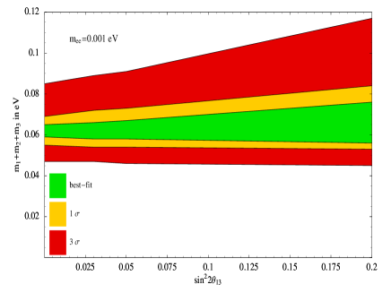
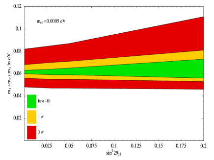
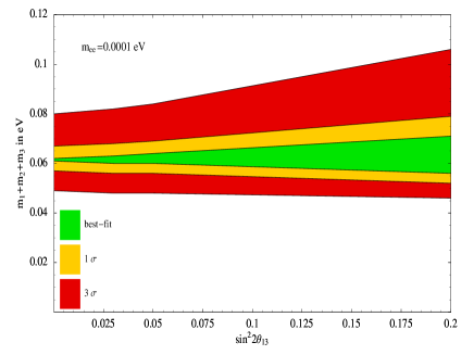
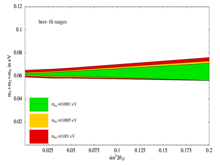
Figure 4: The implied values of the sum of neutrino masses $\Sigma$ (in eV) for the normal mass ordering as a function of $\sin^{2}2\theta_{13}$. Shown are different values for $\left|m_{ee}\right|$ (using the current best-fit, 1 and $3\sigma$ ranges of the oscillation parameters).

3.3 Interplay with Cosmology for very small $\left|m_{ee}\right|$

Let us assume now a very stringent future limit on the effective mass. The only interpretation of this hypothetical, but also realistic, situation is then that the smallest neutrino mass takes values within the “chimney” corresponding to extremely small values of $\left|m_{ee}\right|$. Moreover, the normal mass ordering has to be present, an assertion that might at that point of time already have been confirmed by an independent oscillation experiment. With the indicated values of $m_{1}$, we can go on and calculate the sum of neutrino masses,

$$\Sigma=m_{1}+m_{2}+m_{3}=m_{1}+\sqrt{m_{1}^{2}+\mbox{$\Delta m^{2}_{\odot}$}}+\sqrt{m_{1}^{2}+\mbox{$\Delta m^{2}_{\rm A}$}}~{},$$ (29)

because it is this very quantity, which will also witness some improvement regarding our knowledge about it [27]. Using the current 3$\sigma$ ranges of $\Delta m^{2}_{\odot}$ and $\Delta m^{2}_{\rm A}$, and some values of $\theta_{13}$, gives the ranges for $\Sigma$ displayed in Tables 4 to 6 and in Fig. 4.

One can read off the Tables and the Figure that $\Sigma$ is around 0.1 eV and that its upper limit moderately increases with $\theta_{13}$. Recall that – as shown in the previous Subsection – the width of the “chimney” grows with $\theta_{13}$. The major effect of broadening of the ranges of $\Sigma$ comes from the variation of the oscillation parameter ranges and, as can be seen from the plot with their values fixed to the best-fit values, not from the exact upper limit on $\left|m_{ee}\right|$. Hence, having a limit of 0.001 eV on the effective mass is enough to reach the implied values of $\Sigma$ around 0.1 eV.

The current limit on the sum of neutrino masses lies between 0.42 eV [38] and 1.8 eV [36], depending on the data sets and priors used in the analysis. Future improvement of one order of magnitude is discussed in the literature [27]. Consider now a limit on the effective mass of 0.001 eV. Then, the implied $1\sigma$ range of $\Sigma$ (with such a small limit on $\left|m_{ee}\right|$, the errors on the oscillation parameters are expected to be small, too) is between roughly 0.055 and 0.08 eV. The conservative limit on $\Sigma<1.8$ eV has to be improved merely by a factor of 20 to 40 to fully probe this region. We note finally that a determination of the effective mass above 0.001 eV will lead to testable consequences for cosmology anyway (see e.g. [28]). Here we wish to stress that even a negative search for $\left|m_{ee}\right|$  has some testable impact on cosmology.

3.4 Transition to the quasi-degenerate region

For larger neutrinos masses corresponding to $m_{1}\mathrel{\hbox to0.0pt{\raise 2.20013pt\hbox{$>$}\hss}{\lower 2.20013pt\hbox{$\sim$}}}0.03$ eV, the neutrino masses perform a transition to the “quasi-degenerate regime” in Fig. 3, i.e., corrections to $m_{3}=m_{2}=m_{1}$ are sub-leading. The mass matrix element is given by

$$m_{ee}^{\rm nor}\simeq m_{1}\,\left(c_{12}^{2}\,c_{13}^{2}+s_{12}^{2}\,c_{13}^{2}\,e^{2i\alpha}+s_{13}^{2}\,e^{2i\beta}\right)~{}.$$ (30)

The effective mass scales with $m_{1}$, which in this regime is also the neutrino mass measured in kinematical searches such as KATRIN (in cosmological searches, it would also appear at $m_{1}\simeq\Sigma/3$). In fact, the maximal value of $\left|m_{ee}\right|$ is nothing but $m_{1}$. It holds now $|m_{ee}^{(3)}|\ll|m_{ee}^{(2)}|<|m_{ee}^{(1)}|$ and therefore the minimal value of $\left|m_{ee}\right|$ is given by subtracting the second and third term from the first one, or $\alpha=\beta=\pi/2$ ($--$, see Table 1):

$$\begin{array}[]{c}\mbox{$\left|m_{ee}\right|$}^{\rm nor}_{\rm min}=m_{1}\,c_{12}^{2}\,c_{13}^{2}-\sqrt{m_{1}^{2}+\mbox{$\Delta m^{2}_{\odot}$}}\,s_{12}^{2}\,c_{13}^{2}-\sqrt{m_{1}^{2}+\mbox{$\Delta m^{2}_{\rm A}$}}\,s_{13}^{2}\\[5.69046pt] \simeq m_{1}\,\left(|U_{e1}|^{2}-|U_{e2}|^{2}-|U_{e3}|^{2}\right)=m_{1}\,\frac{\displaystyle 1-\tan^{2}\theta_{12}-2\,\sin^{2}\theta_{13}}{\displaystyle 1+\tan^{2}\theta_{12}}\equiv m_{1}\,f(\theta_{12},\theta_{13})~{}.\end{array}$$ (31)

The function $f(\theta_{12},\theta_{13})$ [30] introduced in this equation has a best-fit value of $0.38$ and a 1(3)$\sigma$ range of $0.32$–$0.44$ ($0.15$–$0.52$). The quantity $m_{1}(1-f(\theta_{12},\theta_{13}))$ defines the width of the band in the quasi-degenerate regime in Fig. 3.

4 The Effective Mass for the Inverted Mass Ordering

For the inverted mass ordering, the smallest neutrino mass is denoted $m_{3}$ and the mass matrix element is given by

$$m_{ee}^{\rm inv}=\sqrt{m_{3}^{2}+\mbox{$\Delta m^{2}_{\rm A}$}}\,c_{12}^{2}\,c_{13}^{2}+\sqrt{m_{3}^{2}+\mbox{$\Delta m^{2}_{\odot}$}+\mbox{$\Delta m^{2}_{\rm A}$}}\,s_{12}^{2}\,c_{13}^{2}\,e^{2i\alpha}+m_{3}\,s_{13}^{2}\,e^{2i\beta}~{}.$$ (32)

The maximal effective mass is – as for the normal mass ordering – obtained by adding the three terms:

$$\left|m_{ee}\right|^{\rm inv}_{\rm max}=\sqrt{m_{3}^{2}+\mbox{$\Delta m^{2}_{\rm A}$}}\,c_{12}^{2}\,c_{13}^{2}+\sqrt{m_{3}^{2}+\mbox{$\Delta m^{2}_{\odot}$}+\mbox{$\Delta m^{2}_{\rm A}$}}\,s_{12}^{2}\,c_{13}^{2}+m_{3}\,s_{13}^{2}~{}.$$ (33)

Finding the minimal $\left|m_{ee}\right|$ is rather easy. With $\mbox{$\Delta m^{2}_{\rm A}$}\gg\mbox{$\Delta m^{2}_{\odot}$}$ one gets for all $m_{3}$

$$\frac{|m_{ee}^{(2)}|}{|m_{ee}^{(1)}|}\simeq\tan^{2}\theta_{12}~{}~{}\mbox{ and }\ \ \frac{|m_{ee}^{(3)}|}{|m_{ee}^{(2)}|}=\frac{m_{3}}{\sqrt{m_{3}^{2}+\mbox{$\Delta m^{2}_{\rm A}$}}}\,\frac{s_{13}^{2}}{c_{12}^{2}\,c_{13}^{2}}~{},$$

which shows that $|m_{ee}^{(2)}/m_{ee}^{(1)}|$ is always smaller and $|m_{ee}^{(3)}/m_{ee}^{(2)}|$ always much smaller than one. Hence, for all values of $m_{3}$ we have $|m_{ee}^{(3)}|\ll|m_{ee}^{(2)}|<|m_{ee}^{(1)}|$ and the minimal value of $\left|m_{ee}\right|$ is obtained by subtracting $|m_{ee}^{(3)}|$ and $|m_{ee}^{(2)}|$ from $|m_{ee}^{(1)}|$, i.e., by choosing $\alpha=\beta=\frac{\pi}{2}$ ($--$, see Table 1):

$$\mbox{$\left|m_{ee}\right|$}^{\rm inv}_{\rm min}=\sqrt{m_{3}^{2}+\mbox{$\Delta m^{2}_{\rm A}$}}\,c_{12}^{2}\,c_{13}^{2}-\sqrt{m_{3}^{2}+\mbox{$\Delta m^{2}_{\odot}$}+\mbox{$\Delta m^{2}_{\rm A}$}}\,s_{12}^{2}\,c_{13}^{2}-m_{3}\,s_{13}^{2}~{}.$$ (34)

The equations (33) and (34) define the upper and the lower line of the band in Fig. 2.

The largest possible $\left|m_{ee}\right|$ is obtained for the largest values of $\Delta m^{2}_{\rm A}$  $\Delta m^{2}_{\odot}$ and $s_{12}^{2}$ as well as for the smallest value of $s_{13}^{2}$. In fact, the dependence of $\mbox{$\left|m_{ee}\right|$}^{\rm inv}_{\rm max}$ on $s_{12}^{2}$ is small, since this parameter enters only via $c_{13}^{2}\,\left(\sqrt{m_{3}^{2}+\mbox{$\Delta m^{2}_{\rm A}$}+\mbox{$\Delta m^{2}_{\odot}$}}-\sqrt{m_{3}^{2}+\mbox{$\Delta m^{2}_{\rm A}$}}\right)\,s_{12}^{2}$, which is only of order $\mbox{$\Delta m^{2}_{\odot}$}/\sqrt{\mbox{$\Delta m^{2}_{\rm A}$}+m_{3}^{2}}$. The smallest value of $\mbox{$\left|m_{ee}\right|$}^{\rm inv}_{\rm max}$ is reached for the largest $\Delta m^{2}_{\odot}$, $s_{13}^{2}$ and $s_{12}^{2}$ as well as the smallest $\Delta m^{2}_{\rm A}$.

4.1 The strictly hierarchical part: $m_{3}\rightarrow 0$

One important case is that of a vanishing lightest neutrino mass, i.e., $m_{3}\rightarrow 0$, the hierarchical regime in Fig. 3. In this case [28, 30, 31],

$$\begin{array}[]{c}m_{ee}^{\rm inv}\simeq\sqrt{\mbox{$\Delta m^{2}_{\rm A}$}}\,c_{13}^{2}\left(c_{12}^{2}+s_{12}^{2}\,e^{2i\alpha}\right)\\[5.69046pt] \mbox{ and }\mbox{$\left|m_{ee}\right|$}^{\rm inv}_{\rm max}\equiv\sqrt{\mbox{$\Delta m^{2}_{\rm A}$}}\,c_{13}^{2}\geq\mbox{$\left|m_{ee}\right|$}^{\rm inv}\geq\sqrt{\mbox{$\Delta m^{2}_{\rm A}$}}\,c_{13}^{2}\cos 2\theta_{12}\equiv\mbox{$\left|m_{ee}\right|$}^{\rm inv}_{\rm min}~{}.\end{array}$$ (35)

From this formula one can see that even for vanishing $s_{13}^{2}$ the band for small neutrino masses has – in contrast to the normal mass ordering – a certain width, given by the allowed range or value of $2\,\sqrt{\mbox{$\Delta m^{2}_{\rm A}$}}\,\sin^{2}\theta_{12}$. For best-fit values (1, 3 $\sigma$ ranges), the width is 0.03 eV (between 0.025 eV and 0.034 eV, 0.018 eV and 0.046 eV, respectively). The dependence on $s_{13}^{2}$ is rather small for the inverted mass ordering, and the effective mass contains information mainly on $\Delta m^{2}_{\odot}$, $\sin^{2}\theta_{12}$ and, in principle, on one of the Majorana phases.

4.2 Transition to the quasi-degenerate region

The transition to the quasi-degenerate regime takes place when $m_{3}\mathrel{\hbox to0.0pt{\raise 2.20013pt\hbox{$>$}\hss}{\lower 2.20013pt\hbox{$\sim$}}}0.03$ eV. If the smallest mass assumes such values, the normal and inverted mass ordering generate identical predictions for the effective mass. The results in this case are therefore identical to the ones for the normal mass ordering treated above in Section 3.4 and can be obtained by replacing $m_{1}$ with $m_{3}$ in the formulae.

5 Normal vs. Inverted Mass Ordering

Having discussed the normal and inverted mass ordering in some detail, we can turn now to a very important aspect of 0$\nu\beta\beta$, namely the possible distinction of the mass orderings [29, 30, 31]. As we have argued in Section 2, the gap between the inverted and normal mass ordering for small masses, i.e., for IH and NH, enjoys some dependence on the value of $\theta_{13}$. By glancing at Fig. 2 or 3, we see that the gap between NH and IH depends also on the precision of the oscillation parameters. For the $3\sigma$ values there is a gap for neutrino masses below a few $10^{-3}$ eV, whereas the best-fit values allow a distinction for neutrino masses below roughly $10^{-2}$ eV. Of course, it is the value of $\theta_{12}$ which plays the main role here [30]. Another point of concern is the uncertainty generated by different calculations of the nuclear matrix elements, which has to be taken into account now.

To do that, we call the nuclear matrix element uncertainty $\zeta$. We have to calculate the difference between the minimal effective mass for the inverted ordering and the maximal effective mass for the normal ordering multiplied with the uncertainty factor $\zeta$:

$$\Delta\mbox{$\left|m_{ee}\right|$}\equiv\mbox{$\left|m_{ee}\right|$}^{\rm inv}_{\rm min}-\zeta\,\mbox{$\left|m_{ee}\right|$}^{\rm nor}_{\rm max}~{}.$$ (36)

The maximal value of $\mbox{$\left|m_{ee}\right|$}^{\rm nor}$ is given in Eq. (18), and the minimal value of $\mbox{$\left|m_{ee}\right|$}^{\rm inv}$ in Eq. (34). Denoting the smallest neutrino mass with $m_{\rm sm}$, we have in general

$$\Delta\mbox{$\left|m_{ee}\right|$}=\mbox{$\left|m_{ee}\right|$}^{\rm inv}_{\rm min}-\zeta\,\mbox{$\left|m_{ee}\right|$}^{\rm nor}_{\rm max}=\left(\sqrt{m_{\rm sm}^{2}+\mbox{$\Delta m^{2}_{\rm A}$}}-\zeta\,m_{\rm sm}\right)\,c_{12}^{2}\,c_{13}^{2}-$$

$$\left(\sqrt{m_{\rm sm}^{2}+\mbox{$\Delta m^{2}_{\odot}$}+\mbox{$\Delta m^{2}_{\rm A}$}}+\zeta\,\sqrt{m_{\rm sm}^{2}+\mbox{$\Delta m^{2}_{\odot}$}}\right)s_{12}^{2}\,c_{13}^{2}-\left(\zeta\,\sqrt{m_{\rm sm}^{2}+\mbox{$\Delta m^{2}_{\rm A}$}}+m_{\rm sm}\right)s_{13}^{2}~{}.$$ (37)

The indicated value of $\Delta\mbox{$\left|m_{ee}\right|$}$ represents the maximal experimental uncertainty in the determination of $\left|m_{ee}\right|$ [30]. For larger uncertainties, distinguishing NH from IH becomes impossible.

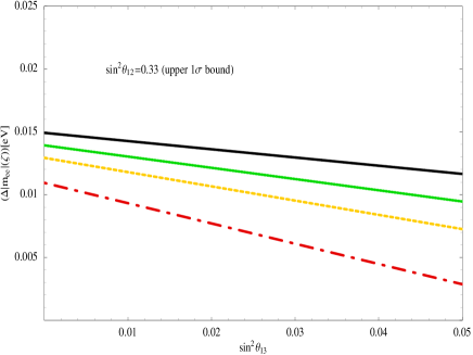
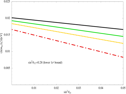
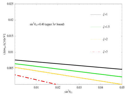
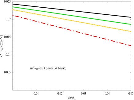
Figure 5: The difference $\Delta\mbox{$\left|m_{ee}\right|$}$ of $\mbox{$\left|m_{ee}\right|$}^{\rm inv}_{\rm min}$ and $\zeta\,\mbox{$\left|m_{ee}\right|$}^{\rm nor}_{\rm max}$ as a function of $\sin^{2}2\theta_{13}$ for an illustrative value of $m_{\rm sm}=0.005$ eV, different sets of oscillation parameters and different nuclear matrix element uncertainty factors $\zeta$.

The variation of $\Delta\mbox{$\left|m_{ee}\right|$}$ with $\theta_{13}$ is only slow, as a function of $s_{13}^{2}$ or $\sin^{2}2\theta_{13}$ it is basically a monotonously decreasing line starting from a value roughly given by $\mbox{$\left|m_{ee}\right|$}^{\rm inv}_{\rm min}$. The value of $\zeta$ effectively increases the negative slope of this line.

The order of magnitude of $\Delta\mbox{$\left|m_{ee}\right|$}$ is generically $\sqrt{\mbox{$\Delta m^{2}_{\rm A}$}}\,\cos^{2}\theta_{13}$. This can be seen, for instance, when we define the small quantities

$$R\equiv\frac{\mbox{$\Delta m^{2}_{\odot}$}}{\mbox{$\Delta m^{2}_{\rm A}$}}~{}~{}\mbox{ and }~{}~{}\eta\equiv\frac{m_{\rm sm}}{\sqrt{\mbox{$\Delta m^{2}_{\rm A}$}}}~{},$$

which allow to rewrite Eq. (37) as

$$\begin{array}[]{c}\Delta\mbox{$\left|m_{ee}\right|$}=\sqrt{\mbox{$\Delta m^{2}_{\rm A}$}}\,c_{13}^{2}\,\left(c_{12}^{2}\,\left(\sqrt{1-\eta^{2}}-\eta\,\zeta\right)-s_{12}^{2}\,\left(\sqrt{1-\eta^{2}+R}+\zeta\,\sqrt{R+\eta^{2}}\right)\right.\\[5.69046pt] \left.-\left(\eta+\sqrt{1-\eta^{2}}\,\zeta\right)\,\tan^{2}\theta_{13}\right)~{}.\end{array}$$ (38)

At zeroth order in all small quantities $R$, $\eta$ and $\theta_{13}$, we have $\Delta\mbox{$\left|m_{ee}\right|$}\simeq\sqrt{\mbox{$\Delta m^{2}_{\rm A}$}}\,\cos 2\theta_{12}$, which is nothing but $\mbox{$\left|m_{ee}\right|$}^{\rm inv}_{\rm min}$.

Using $\mbox{$\Delta m^{2}_{\rm A}$}+\mbox{$\Delta m^{2}_{\odot}$}\simeq\mbox{$\Delta m^{2}_{\rm A}$}$ and taking the limit $m_{\rm sm}\rightarrow 0$, we get from Eq. (37)

$$\Delta\mbox{$\left|m_{ee}\right|$}(m_{\rm sm}\rightarrow 0)\simeq\sqrt{\mbox{$\Delta m^{2}_{\rm A}$}}\left(c_{13}^{2}\,(c_{12}^{2}-s_{12}^{2})-\zeta\,s_{13}^{2}\right)-\zeta\,\sqrt{\mbox{$\Delta m^{2}_{\odot}$}}\,s_{12}^{2}\,c_{13}^{2}~{}.$$ (39)

For no uncertainty, i.e., if $\zeta=1$, and for the current best-fit values of the oscillation parameters, this function monotonously decreases from 15.0 meV for $\theta_{13}=0$ to 12.0 meV for $s_{13}^{2}=0.05$. If $\zeta=2$, then it decreases from 12.3 meV for $\theta_{13}=0$ to 7.0 meV for $s_{13}^{2}=0.05$. As noted in Ref. [30], the dependence on $\theta_{12}$ of $\Delta\mbox{$\left|m_{ee}\right|$}$ is rather strong. We give a few numerical examples, obtained for a vanishing smallest neutrino mass: if we take $\zeta=1$ and $\sin^{2}\theta_{12}=0.24$ (lower 3$\sigma$ value), then $\Delta\mbox{$\left|m_{ee}\right|$}$ decreases from 22.3 meV for $\theta_{13}=0$ to 18.8 meV for $s_{13}^{2}=0.05$. For the same $\sin^{2}\theta_{12}$ and $\zeta=2$, its values are 14.4 meV ($\theta_{13}=0$) and 5.8 meV ($s_{13}^{2}=0.05$). For $\sin^{2}\theta_{12}=0.40$ (upper 3$\sigma$ value) in turn, $\Delta\mbox{$\left|m_{ee}\right|$}$ decreases from 5.8 meV for $\theta_{13}=0$ to 3.2 meV for $s_{13}^{2}=0.05$ if $\zeta=1$, while for $\zeta=2$ it starts at 2.3 meV and crosses zero for $s_{13}^{2}\simeq 0.024$. Values of $\Delta\mbox{$\left|m_{ee}\right|$}$ equal to or less than zero mean that one cannot distinguish the normal from the inverted hierarchy anymore.

For $\theta_{13}=0$ the variation of the oscillation parameters gives a range of $\Delta\mbox{$\left|m_{ee}\right|$}$ from 12 to 20 meV ($1\sigma$) or 4 to 28 meV ($3\sigma$) for $\zeta=1$ and from 9 to 17 meV ($1\sigma$) or 0 to 26 meV ($3\sigma$) for $\zeta=2$ (within the parameter range of the oscillation parameters $\Delta\mbox{$\left|m_{ee}\right|$}$ can become less than zero). Fixing the oscillation parameters to their best-fit values and varying $\zeta$ from 1 to 5 leads to a range of $\Delta\mbox{$\left|m_{ee}\right|$}$ from 15 to 4 meV. For $\sin^{2}2\theta_{13}=0.02$ (0.2) the range is 14.8 to 2.8 (11.8 to 0) meV.

For an illustrative value of $m_{\rm sm}=0.005$ eV and for different $\sin^{2}\theta_{12}$ and $\zeta$ we show $\Delta\mbox{$\left|m_{ee}\right|$}$ as a function of $\sin^{2}\theta_{13}$ in Fig. 5. We see that if the true value of $\sin^{2}\theta_{12}$ is not too far away from its current best-fit value and if $\zeta\mathrel{\hbox to0.0pt{\raise 2.20013pt\hbox{$<$}\hss}{\lower 2.20013pt\hbox{$\sim$}}}2$, then $\Delta\mbox{$\left|m_{ee}\right|$}$ lies always around 0.01 eV unless $\theta_{13}$ is very close to its current upper limit. If $\sin^{2}\theta_{12}$ is on the upper side of its allowed range or $\zeta\mathrel{\hbox to0.0pt{\raise 2.20013pt\hbox{$>$}\hss}{\lower 2.20013pt\hbox{$\sim$}}}2$, then rather small values of $\Delta\mbox{$\left|m_{ee}\right|$}$ are implied. We remark that recent investigations seem to indicate that indeed $\zeta\mathrel{\hbox to0.0pt{\raise 2.20013pt\hbox{$<$}\hss}{\lower 2.20013pt\hbox{$\sim$}}}2$ [39].

An interesting point worth stressing is the complementary role played by 0$\nu\beta\beta$ and oscillation experiments in what regards the determination of the neutrino mass hierarchy. As we discussed here in some detail, the gap $\Delta\mbox{$\left|m_{ee}\right|$}$ between IH and NH decreases for increasing values of $\theta_{13}$. For oscillation experiments on the other hand, one typically uses matter effects on $\theta_{13}$ to pin down the hierarchy. Consequently, in case of zero $\theta_{13}$ these efforts are doomed. In principle it will still be possible to determine the hierarchy in oscillation experiments, but this typically requires a precision measurement of $\Delta m^{2}_{\rm A}$ on a level of $\Delta m^{2}_{\odot}$ [40], which is quite challenging. Hence, the larger $\theta_{13}$, the easier it will be to measure the mass ordering, i.e., the sign of $m_{3}^{2}-m_{1}^{2}$. From this point of view, both types of experiments are complementary. Let us however not shut off from view that the identification of the sign of $m_{3}^{2}-m_{1}^{2}$ via 0$\nu\beta\beta$ depends on the fact that the smallest neutrino mass indeed should be small, say, $m_{\rm sm}\mathrel{\hbox to0.0pt{\raise 2.20013pt\hbox{$<$}\hss}{\lower 2.20013pt\hbox{$\sim$}}}0.01$ eV. However, most GUT based models predicting neutrino parameters predict a normal hierarchy with such light neutrino masses (for a summary of possibilities and models, see for instance [1, 30]). If a model incorporates the inverted mass ordering, then stability under radiative corrections demands usually the flavor symmetry $L_{e}-L_{\mu}-L_{\tau}$ [41] to play a role, and consequently, even after breaking the symmetry, the smallest mass is very light, too.

Moreover, any extraction of information from 0$\nu\beta\beta$ has some intrinsic model dependence. The most important one is the assertion that neutrinos are Majorana particles, which however has more than only solid theoretical foundation. Then again, there are several diagrams of Physics beyond the Standard Model which in principle can mediate neutrino-less double beta decay. However, no such New Physics candidate has shown up so far, and the indisputable evidence for neutrino oscillations indicates that the neutrino-mass-mediated channel of 0$\nu\beta\beta$ is present. Since any Feynman diagram leading to 0$\nu\beta\beta$ automatically generates a (loop-suppressed) Majorana mass term for the neutrinos [42], one would have to explain why massive neutrino are a sub-leading contribution to 0$\nu\beta\beta$ but the other New Physics responsible for it does not show up elsewhere.

6 Conclusions

Future measurements will improve the sensitivity for $\sin^{2}2\theta_{13}$ by at least one order of magnitude within the next years. At the same time there will be considerable improvements in the determination of the absolute neutrino mass scale from neutrino-less double beta decay and from cosmology. We discussed in this paper the interplay of these improvements. Especially, we showed that a measurement or an improved limit of $\theta_{13}$ is very important for the separation and for the precise form of the normal and inverted hierarchy solution for hierarchical neutrino masses. We demonstrated that for todays largest possible values of $\theta_{13}$, the normal and inverted hierarchy regions overlap. An improvement of $\theta_{13}$ is especially important to be able to fully exclude or probe the inverted mass hierarchy with next generation of 0$\nu\beta\beta$ experiments like GERDA, CUORE or MAJORANA. In addition, we showed that in the case of a normal hierarchy, arbitrarily small values of the effective neutrino mass are allowed for these largest possible values of $\theta_{13}$. For intermediate values of the absolute neutrino mass scale we showed that the width of the “chimney” depends sizably on $\theta_{13}$. The anticipated improvement by one order of magnitude will make this “chimney” rather narrow. Even though the chimney exists for arbitrarily small values of $\theta_{13}$, its width becomes so narrow that it would correspond to rather specifically chosen parameter values. If 0$\nu\beta\beta$ experiments reach a sensitivity for $|m_{ee}|\mathrel{\hbox to0.0pt{\raise 2.20013pt\hbox{$<$}\hss}{\lower 2.20013pt\hbox{$\sim$}}}10^{-3}$ eV, and if neutrinos are Majorana particles, then only the “chimney” remains as allowed parameter space, where again the width is considerably reduced by future measurements of $\theta_{13}$. The width of the “chimney” is also relevant for future improvements of the cosmological mass bounds for neutrinos. The value of $\theta_{13}$ sets an upper bound for the sum of neutrino masses, which may be reached by the cosmological bounds. This could lead to interesting scenarios depending on whether 0$\nu\beta\beta$ experiments, cosmological determinations and/or improved $\theta_{13}$ measurements see a signal or improve the limits, respectively. In the region of degenerate neutrino masses we found that improved values of $\theta_{13}$ reduce the range of allowed masses on the lower side of $|m_{ee}|$. Altogether we demonstrated, that there is a sizable interplay of the improvements expected in 0$\nu\beta\beta$ experiments, improved cosmological bounds and upcoming $\theta_{13}$ measurements.

Acknowledgments: This work has been supported by SFB375 (M.L.) and project number RO–2516/3–1 (W.R.) of Deutsche Forschungsgemeinschaft. We would like to thank M. Goodman for discussions and J. Kopp for help concerning computer problems.

References

- [1] R. N. Mohapatra et al., hep-ph/0412099; hep-ph/0510213.
- [2] C. Aalseth et al., hep-ph/0412300.
- [3] P. Huberet al., Phys. Rev. D 70, 073014 (2004), hep-ph/0403068.
- [4] Y. Shitov [NEMO Collaboration], nucl-ex/0405030.
- [5] S. Capelli, hep-ex/0505045 and Phys. Rev. Lett. 95, 142501 (2005), hep-ex/0501034.
- [6] R. Ardito et al., hep-ex/0501010.
- [7] R. Gaitskell et al. [Majorana Collaboration], nucl-ex/0311013.
- [8] I. Abt et al., hep-ex/0404039.
- [9] M. Danilov et al., Phys. Lett. B 480, 12 (2000), hep-ex/0002003.
- [10] H. Ejiri et al., Phys. Rev. Lett. 85, 2917 (2000), nucl-ex/9911008.
- [11] K. Zuber, Phys. Lett. B 519, 1 (2001), nucl-ex/0105018.
- [12] N. Ishihara, T. Ohama and Y. Yamada, Nucl. Instrum. Meth. A 373, 325 (1996).
- [13] S. Yoshida et al., Nucl. Phys. Proc. Suppl. 138, 214 (2005).
- [14] G. Bellini et al., Eur. Phys. J. C 19, 43 (2001), nucl-ex/0007012.
- [15] B. Pontecorvo, Zh. Eksp. Teor. Fiz. 33, 549 (1957) and 34, 247 (1957); Z. Maki, M. Nakagawa and S. Sakata, Prog. Theor. Phys. 28, 870 (1962).
- [16] S. M. Bilenky, J. Hosek and S. T. Petcov, Phys. Lett. B 94, 495 (1980); M. Doi et al., Phys. Lett. B 102, 323 (1981); J. Schechter and J. W. F. Valle, Phys. Rev. D 23, 1666 (1981).
- [17] H. V. Klapdor-Kleingrothaus et al., Eur. Phys. J. A 12, 147 (2001), hep-ph/0103062.
- [18] C. E. Aalseth et al. [IGEX Collaboration], Phys. Rev. D 65, 092007 (2002), hep-ex/0202026.
- [19] H. V. Klapdor-Kleingrothaus et al., Mod. Phys. Lett. A 16, 2409 (2001), hep-ph/0201231; C. E. Aalseth et al., Mod. Phys. Lett. A 17, 1475 (2002), hep-ex/0202018; H. L. Harney, hep-ph/0205293; H. V. Klapdor-Kleingrothaus, hep-ph/0205228; F. Feruglio, A. Strumia and F. Vissani, Nucl. Phys. B 637, 345 (2002), hep-ph/0201291, [Addendum-ibid. B 659, 359 (2003)]; H. V. Klapdor-Kleingrothaus et al., Phys. Lett. B 586, 198 (2004), hep-ph/0404088.
- [20] E. Ables et al. (MINOS) FERMILAB-PROPOSAL-P-875.
- [21] P. Aprili et al. (ICARUS) CERN-SPSC-2002-027.
- [22] D. Duchesneau (OPERA), Nucl. Phys. Proc. Suppl. 123, 279 (2003), hep-ex/0209082.
- [23] F. Ardellier et al., hep-ex/0405032.
- [24] Y. Itow et al., hep-ex/0106019.
- [25] D. Ayres et al., hep-ex/0210005.
- [26] A. Osipowicz et al. [KATRIN Collaboration], hep-ex/0109033.
- [27] For an overview see S. Hannestad, Nucl. Phys. Proc. Suppl. 145, 313 (2005), hep-ph/0412181.
- [28] S. M. Bilenky et al., Phys. Rev. D 54, 4432 (1996), hep-ph/9604364; Phys. Lett. B 465, 193 (1999), hep-ph/9907234; H. V. Klapdor-Kleingrothaus, H. Päs and A. Y. Smirnov, Phys. Rev. D 63, 073005 (2001), hep-ph/0003219; W. Rodejohann, Nucl. Phys. B 597, 110 (2001), hep-ph/0008044; S. M. Bilenky, S. Pascoli and S. T. Petcov, Phys. Rev. D 64, 053010 (2001), hep-ph/0102265; V. Barger et al., Phys. Lett. B 532, 15 (2002), hep-ph/0201262; F. Feruglio, A. Strumia and F. Vissani, in Ref. [19]; H. Minakata and H. Sugiyama, Phys. Lett. B 567, 305 (2003), hep-ph/0212240; F. R. Joaquim, Phys. Rev. D 68, 033019 (2003), hep-ph/0304276; G. L. Fogli et al., Phys. Rev. D 70, 113003 (2004), hep-ph/0408045.
- [29] Some recent works are e.g. S. Pascoli and S. T. Petcov, Phys. Lett. B 544, 239 (2002), hep-ph/0205022; S. Pascoli, S. T. Petcov and W. Rodejohann, Phys. Lett. B 558, 141 (2003), hep-ph/0212113; H. Murayama and C. Pena-Garay, Phys. Rev. D 69, 031301 (2004), hep-ph/0309114; A. de Gouvea and J. Jenkins, hep-ph/0507021; S. M. Bilenky et al., Phys. Rev. D 72, 053015 (2005), hep-ph/0507260.
- [30] S. Choubey and W. Rodejohann, Phys. Rev. D 72, 033016 (2005), hep-ph/0506102.
- [31] S. Pascoli, S. T. Petcov and T. Schwetz, Nucl. Phys. B 734, 24 (2006), hep-ph/0505226.
- [32] S. T. Petcov, New J. Phys. 6, 109 (2004).
- [33] T. Schwetz, hep-ph/0510331.
- [34] W. Rodejohann, Phys. Rev. D 62, 013011 (2000); J. Phys. G 28, 1477 (2002); K. Zuber, hep-ph/0008080; A. Atre, V. Barger and T. Han, Phys. Rev. D 71, 113014 (2005), hep-ph/0502163.
- [35] L. Wolfenstein, Phys. Lett. B 107, 77 (1981); S. M. Bilenky, N. P. Nedelcheva and S. T. Petcov, Nucl. Phys. B 247, 61 (1984); B. Kayser, Phys. Rev. D 30, 1023 (1984).
- [36] M. Tegmark et al., Phys. Rev. D 69, 103501 (2004), astro-ph/0310723.
- [37] S. Pascoli, S. T. Petcov and L. Wolfenstein, Phys. Lett. B 524, 319 (2002), hep-ph/0110287; Z. Z. Xing, Phys. Rev. D 68, 053002 (2003), hep-ph/0305195.
- [38] U. Seljak et al., Phys. Rev. D 71, 103515 (2005), astro-ph/0407372.
- [39] V. A. Rodin, A. Faessler, F. Simkovic and P. Vogel, nucl-th/0503063.
- [40] A. de Gouvea, J. Jenkins and B. Kayser, hep-ph/0503079; H. Nunokawa, S. Parke and R. Zukanovich Funchal, Phys. Rev. D 72, 013009 (2005), hep-ph/0503283; A. de Gouvea and W. Winter, hep-ph/0509359.
- [41] S. T. Petcov, Phys. Lett. B 110, 245 (1982).
- [42] J. Schechter and J. W. F. Valle, Phys. Rev. D 25, 2951 (1982).