[3cm]hep-ph/0512137
December, 2005

The Dilepton $Q_{T}$ Spectrum in
Transversely Polarized Drell-Yan Process in QCD

Abstract

We discuss the transverse momentum $Q_{T}$ distribution of Drell-Yan pair, produced in collisions of transversely polarized protons. We calculate the transversely polarized Drell-Yan cross section up to ${\cal O}(\alpha_{s})$ in the dimensional regularization, which gives QCD prediction at large $Q_{T}$. For small $Q_{T}$, we include all-orders resummation of large logarithms due to emission of soft gluons up to next-to-leading logarithmic accuracy. At intermediate $Q_{T}$, the resummation formula is matched with the fixed-order $\alpha_{s}$ perturbative results in a systematic way, and we derive the cross section with uniform accuracy over the entire range of $Q_{T}$.

Hard processes with polarized beams and/or target enable us to study spin-dependent dynamics of QCD. The helicity distribution $\Delta q(x)$ of quarks inside nucleon has been measured in polarized DIS experiments, and also $\Delta G(x)$ of gluon has been estimated from the scaling violations of them. On the other hand, the transversity distribution $\delta q(x)$, i.e. the distribution of transversely polarized quarks inside transversely polarized nucleon, cannot be measured in the inclusive DIS due to its chiral-odd nature,[1] and remains as the last unknown distribution at the leading twist. Transversely polarized Drell-Yan (tDY) process is one of the processes where $\delta q(x)$ can be measured, and has been undertaken at RHIC-Spin experiment.[2]

We develop the QCD prediction of tDY cross section, $d\sigma/dQ^{2}dQ_{T}^{2}dyd\phi$, differential in the transverse momentum $Q_{T}$ and rapidity $y$ of the produced lepton pair, as well as in the dilepton invariant mass $Q$ and in the azimuthal angle $\phi$ of one of the leptons with respect to the incoming nucleon’s spin axis. Although this $Q_{T}$- and $y$-differential cross section is fundamental in view of comparison with experiment, the corresponding formula has been unknown so far even in the leading order (LO) in QCD: the lepton-pair production with finite $Q_{T}$ via the Drell-Yan mechanism has to be accompanied by the radiation of at least one recoiling parton, so the LO term of the cross section is of ${\cal O}(\alpha_{s})$. The corresponding one-loop calculation of the LO term requires the phase space integration separating out the relevant transverse degrees of freedom, to extract the $\cos(2\phi)$ dependence which is characteristic of the spin-dependent cross section of tDY.[1] In the dimensional regularization, in particular, the relevant phase space integration in $D$-dimension is rather cumbersome compared with unpolarized and longitudinally polarized cases. Furthermore, at small $Q_{T}$ (“edge regions of the phase space”), the radiation of soft gluon produces large “recoil logs” that spoil fixed-order perturbation theory, and the corresponding logarithmically enhanced contributions have to be resummed to all orders in $\alpha_{s}$. Previous works treated $Q_{T}$- and/or $y$-integrated tDY cross sections to fixed-order $\alpha_{s}$, employing the massive gluon scheme[3] and the dimensional reduction scheme[4] (see also Refs. WV:98,MSSV:98). In this Letter, we compute the $Q_{T}$- and $y$-differential cross section of tDY in the LO (${\cal O}(\alpha_{s})$) in the dimensional regularization scheme. Then the result is consistently combined with the soft gluon resummation of logarithmically enhanced contributions for small $Q_{T}$ up to next-to-leading logarithmic (NLL) accuracy, and we derive the first complete result of the well-defined tDY differential cross section in the $\overline{\rm MS}$ scheme for all regions of $Q_{T}$ at the “${\rm NLL}+{\rm LO}$” level.

We first consider the tDY cross section to ${\cal O}(\alpha_{s})$: $h_{1}(P_{1},s_{1})+h_{2}(P_{2},s_{2})\rightarrow l(k_{1})+\bar{l}(k_{2})+X$, where $h_{1},h_{2}$ denote nucleons with momentum $P_{1},P_{2}$ and transverse spin $s_{1},s_{2}$, and $Q=k_{1}+k_{2}$ is the 4-momentum of DY pair. Based on QCD factorization, the spin-dependent cross section $\Delta_{T}d\sigma\equiv(d\sigma(s_{1},s_{2})-d\sigma(s_{1},-s_{2}))/2$ is given as a convolution, $\Delta_{T}d\sigma=\int dx_{1}dx_{2}\delta H(x_{1},x_{2};\mu_{F}^{2})\Delta_{T}d\hat{\sigma}(\mu_{F}^{2})$, where $\mu_{F}$ is the factorization scale, $\delta H(x_{1},x_{2};\mu_{F}^{2})=\sum_{i}e_{i}^{2}[\delta q_{i}(x_{1};\mu_{F}^{2})\delta\bar{q}_{i}(x_{2};\mu_{F}^{2})+\delta\bar{q}_{i}(x_{1};\mu_{F}^{2})\delta q_{i}(x_{2};\mu_{F}^{2})]$ is the product of transversity distributions of the two nucleons, and $\Delta_{T}d\hat{\sigma}(\mu_{F}^{2})=(d\hat{\sigma}(s_{1},s_{2};\mu_{F}^{2})-d\hat{\sigma}(s_{1},-s_{2};\mu_{F}^{2}))/2$ is the corresponding partonic cross section. Note that, at the leading twist level, the gluon does not contribute to the transversely polarized, chiral-odd process, corresponding to helicity-flip by one unit. We compute the one-loop corrections to $\Delta_{T}d\hat{\sigma}(\mu_{F}^{2})$, which involve the virtual gluon corrections and the real gluon emission contributions, e.g., $q(p_{1},s_{1})+\bar{q}(p_{2},s_{2})\to l(k_{1})+\bar{l}(k_{2})+g$, with $p_{i}=x_{i}P_{i}$. We regularize the infrared divergence in $D=4-2\epsilon$ dimension, and employ naive anticommuting $\gamma_{5}$ which is a usual prescription in the transverse spin channel.[5] In the $\overline{\rm MS}$ scheme, we obtain for the differential cross section

$$\frac{\Delta_{T}d\sigma}{dQ^{2}dQ_{T}^{2}dyd\phi}=\cos{(2\phi)}\frac{\alpha^{2}}{3\,N_{c}\,S\,Q^{2}}\left[X\,(Q_{T}^{2}\,,\,Q^{2}\,,\,y)+Y\,(Q_{T}^{2}\,,\,Q^{2}\,,\,y)\right],$$ (1)

with $S=(P_{1}+P_{2})^{2}$, and the rapidity $y=(1/2)\ln[(Q^{0}+Q^{3})/(Q^{0}-Q^{3})]$ where $Q^{3}$ is the component of the virtual photon momentum $Q^{\mu}$ along the direction of the colliding beam in the nucleon-nucleon CM system. We have decomposed the RHS into two parts: the function $X$ contains all terms that are singular as $Q_{T}\rightarrow 0$, while $Y$ is of ${\cal O}(\alpha_{s})$ and finite at $Q_{T}=0$. Writing $X=X^{(0)}+X^{(1)}$ as the sum of ${\cal O}(\alpha_{s}^{0})$ and ${\cal O}(\alpha_{s}^{1})$ contributions, we have $X^{(0)}=\delta H(x_{1}^{0}\,,\,x_{2}^{0}\,;\,\mu_{F}^{2})\ \delta(Q_{T}^{2})$, and

$$X^{(1)} = \frac{\alpha_{s}(\mu_{R}^{2})}{2\pi}C_{F}\Biggl{\{}\delta H(x_{1}^{0}\,,\,x_{2}^{0}\,;\,\mu_{F}^{2})\left[\,2\left(\frac{\ln(Q^{2}/Q_{T}^{2})}{Q_{T}^{2}}\right)_{+}-\frac{3}{(Q_{T}^{2})_{+}}+\left(\pi^{2}-8\right)\delta(Q_{T}^{2})\right]$$

$$\!\!\!\!\!\!\!\!\!\!\!\!\!\!\!\!\!+ \!\!\!\!\!\!\!\!\left(\frac{1}{(Q_{T}^{2})_{+}}+\delta(Q_{T}^{2})\ln\frac{Q^{2}}{\mu_{F}^{2}}\right)\!\!\!\left[\int^{1}_{x_{1}^{0}}\frac{dz}{z}\delta P_{qq}^{(0)}(z)\ \delta H\left(\frac{x_{1}^{0}}{z},x_{2}^{0};\ \mu_{F}^{2}\right)+(x_{1}^{0}\leftrightarrow x_{2}^{0})\right]\Biggr{\}},$$ (2)

where $\mu_{R}$ is the renormalization scale, $x_{1}^{0}=\sqrt{\tau}\ e^{y},x_{2}^{0}=\sqrt{\tau}\ e^{-y}$ are the relevant scaling variables with $\tau=Q^{2}/S$, and $\delta P_{qq}^{(0)}(z)=2z/(1-z)_{+}+(3/2)\,\delta(1-z)$ is the LO transverse splitting function.[9, 5] The “+” distribution to regulate the singularity at $Q_{T}=0$ is defined such that $\int_{0}^{p_{T}^{2}}dQ_{T}^{2}([\ln^{n}(Q^{2}/Q_{T}^{2})]/Q_{T}^{2})_{+}=-(1/[n+1])\ln^{n+1}(Q^{2}/p_{T}^{2})$. For the $Y$-term of (1),

$$Y = \frac{\alpha_{s}(\mu_{R}^{2})}{\pi}\,C_{F}\left\{\left[\,\frac{2}{Q^{2}}\,-\,\frac{3}{Q_{T}^{2}}\,\ln\left(1+\frac{Q_{T}^{2}}{Q^{2}}\right)\right]\int^{1}_{\sqrt{\tau_{+}}\,e^{y}}\,\frac{dx_{1}}{x_{1}-x_{1}^{+}}\,\delta H(x_{1}\,,\,x_{2}^{*};\mu_{F}^{2})\,\frac{\tau}{x_{1}x_{2}^{*}}\right.$$ (3)

$$+ \left.\frac{1}{Q_{T}^{2}}\,\left[\int dx_{1}\,\delta H_{1}+\frac{1}{2}\delta H(x_{1}^{0}\,,\,x_{2}^{0};\mu_{F}^{2})\,\ln\frac{(1-x_{1}^{+})(1-x_{2}^{+})}{(1-x_{1}^{0})(1-x_{2}^{0})}\right]\right\}+\left(y\rightarrow-y\right)\ ,$$

where we used the shorthand notation for the integral that vanishes for $Q_{T}=0$,

$$\int dx_{1}\delta H_{1} \equiv \int^{1}_{\sqrt{\tau_{+}}\,e^{y}}\ \,\frac{dx_{1}}{x_{1}-x_{1}^{+}}\left[\delta H(x_{1}\,,\,x_{2}^{*};\,\mu_{F}^{2})\,\frac{\tau}{x_{1}x_{2}^{*}}-\delta H(x_{1}^{0}\,,\,x_{2}^{0};\,\mu_{F}^{2})\right]$$

$$\hskip 56.9055pt-\int^{1}_{x_{1}^{0}}\ \,\frac{dx_{1}}{x_{1}-x_{1}^{0}}\left[\delta H(x_{1}\,,\,x_{2}^{0};\,\mu_{F}^{2})\,\frac{x_{1}^{0}}{x_{1}}-\delta H(x_{1}^{0}\,,\,x_{2}^{0};\,\mu_{F}^{2})\right]\ .$$

and defined the variables, $\sqrt{\tau_{+}}=\sqrt{Q_{T}^{2}/S}+\sqrt{\tau+Q_{T}^{2}/S}$, $x_{1,2}^{+}=x_{1,2}^{0}\sqrt{1+Q_{T}^{2}/Q^{2}}$, $x_{2}^{*}=(x_{1}x_{2}^{+}-x_{1}^{0}x_{2}^{0})/(x_{1}-x_{1}^{+})$, following Ref. AEGM:84. Note that $x_{1,2}^{+}\rightarrow x_{1,2}^{0}$ and $x_{2}^{*}\rightarrow x_{2}^{0}$ as $Q_{T}\rightarrow 0$, and all terms in (3) are finite when $Q_{T}\rightarrow 0$.

Eq. (1) with (2) and (3) gives the first result for the differential cross section to ${\cal O}(\alpha_{s})$ in the $\overline{\rm MS}$ scheme. The result is invariant under the replacement $y\rightarrow-y$ as it should be. We note that, integrating (1) over $Q_{T}$, our result coincides with the corresponding $Q_{T}$-integrated cross sections obtained in previous works employing massive gluon scheme[3] and dimensional reduction scheme,[4] via the scheme transformation relation[5] (see also Ref. MSSV:98). For $Q_{T}^{2}>0$, $X^{(0)}$ vanishes. Also, the terms proportional to $\delta(Q_{T}^{2})$ in (2), including those associated with the + distribution $([\ln^{n}(Q^{2}/Q_{T}^{2})]/Q_{T}^{2})_{+}$, do not contribute. The cross section (1) in this case is of ${\cal O}(\alpha_{s})$, and gives the LO QCD prediction of tDY at the large-$Q_{T}$ region:

$$\frac{\Delta_{T}d\sigma^{\rm LO}}{dQ^{2}dQ_{T}^{2}dyd\phi}=\cos{(2\phi)}\frac{\alpha^{2}}{3\,N_{c}\,S\,Q^{2}}\left[\left.X^{(1)}(Q_{T}^{2},Q^{2},y)\right|_{Q_{T}^{2}>0}+Y(Q_{T}^{2},Q^{2},y)\right].$$ (5)

The cross section (1) becomes very large when $Q_{T}\ll Q$, due to the terms behaving $\sim\alpha_{s}\ln(Q^{2}/Q_{T}^{2})/Q_{T}^{2}$ and $\sim\alpha_{s}/Q_{T}^{2}$ in (2). Actually, similar large “recoil logs” appear in each order of perturbation theory as $\alpha_{s}^{n}\ln^{2n-1}(Q^{2}/Q_{T}^{2})/Q_{T}^{2}$, $\alpha_{s}^{n}\ln^{2n-2}(Q^{2}/Q_{T}^{2})/Q_{T}^{2}$, and so on, corresponding to LL, NLL, and higher contributions, respectively,[6, 7] and the resummation of those logarithmically enhanced contributions to all orders is necessary to obtain a well-defined, finite prediction for the cross section. We work out this up to the NLL accuracy, based on the general formulation[7] of the $Q_{T}$ resummation. This can be carried out in the impact parameter $b$ space, conjugate to the $Q_{T}$ space: the singular term $X$ of (1) is modified into the corresponding resummed component, which is expressed as the Fourier transform back to the $Q_{T}$ space. As a result, the first term in the RHS of (1) is replaced by

$$\frac{\Delta_{T}d\sigma^{\rm NLL}}{dQ^{2}dQ_{T}^{2}dyd\phi}=\cos (2\phi)\frac{\alpha^{2}}{3\,N_{c}\,S\,Q^{2}}\sum_{i}e_{i}^{2}\int_{0}^{\infty}db\frac{b}{2}J_{0}(bQ_{T})$$

$$\times e^{\,S(b,Q)} \left[(C_{qq}\otimes\delta q_{i})\left(x_{1}^{0},\frac{b_{0}^{2}}{b^{2}}\right)(C_{\bar{q}\bar{q}}\otimes\delta\bar{q}_{i})\left(x_{2}^{0},\frac{b_{0}^{2}}{b^{2}}\right)+(x_{1}^{0}\leftrightarrow x_{2}^{0})\right].$$ (6)

Here $J_{0}(bQ_{T})$ is a Bessel function, $b_{0}=2e^{-\gamma_{E}}$ with $\gamma_{E}$ the Euler constant, and the large logarithmic corrections are resummed into the Sudakov factor $e^{S(b,Q)}$ with
$S(b,Q)=-\int_{b^{2}_{0}/b^{2}}^{Q^{2}}(d\kappa^{2}/\kappa^{2})\left\{A_{q}(\alpha_{s}(\kappa^{2}))\ln(Q^{2}/\kappa^{2})+B_{q}(\alpha_{s}(\kappa^{2}))\right\}$. The functions $A_{q}$, $B_{q}$ as well as the coefficient functions $C_{qq},C_{\bar{q}\bar{q}}$, are perturbatively calculable: we get $A_{q}(\alpha_{s})=\sum_{n=1}^{\infty}\left(\frac{\alpha_{s}}{2\pi}\right)^{n}A_{q}^{(n)}$, $B_{q}(\alpha_{s})=\sum_{n=1}^{\infty}\left(\frac{\alpha_{s}}{2\pi}\right)^{n}B_{q}^{(n)}$, with

$$A_{q}^{(1)}=2C_{F}\ ,~{}~{}~{}~{}A_{q}^{(2)}=2C_{F}\left\{\left(\frac{67}{18}-\frac{\pi^{2}}{6}\right)C_{G}-\frac{5}{9}N_{f}\right\}\ ,~{}~{}~{}~{}B_{q}^{(1)}=-3C_{F}\ ,\\$$ (7)

at the present accuracy of NLL, and similarly,

$$C_{qq}(z,\alpha_{s})=C_{\bar{q}\bar{q}}(z,\alpha_{s})=\delta(1-z)\left\{1+\frac{\alpha_{s}}{2\pi}C_{F}\left(\frac{\pi^{2}}{2}-4\right)\right\}+{\cal O}(\alpha_{s}^{2})\ .$$ (8)

Here we have utilized a relation[8] between $A_{q}$ and the DGLAP kernels[9, 5] in order to obtain $A_{q}^{(2)}$ of (7).[10] The other contributions of (7), (8) have been determined so that the expansion of the above formula (6) in powers of $\alpha_{s}(\mu_{R}^{2})$ reproduces $X$ with (2) to ${\cal O}(\alpha_{s})$. Our results (7) are consistent with the fact that the LL ($A_{q}^{(1)}$) and NLL ($A_{q}^{(2)},B_{q}^{(1)}$) contributions are universal (process-independent).[11]

Eq. (6) with (7), (8) satisfies the evolution equation controlled by renormalization group,[7] and is formally perfect. As emphasized in Refs. LKSV:01,BCDeG:03 for the unpolarized processes, however, several “reorganization” in the formula of this type is necessary for its consistent evaluation up to required accuracy, to treat properly the $b$ integration of (6) that involves too short as well as long distance. In the $b$ space, $L\equiv\ln(Q^{2}b^{2}/b_{0}^{2})$ plays role of the relevant large logarithm, with $b\sim 1/Q_{T}$. Expressing the $b$ dependence of the second line in (6) as the corresponding $L$ dependence, and systematically organizing those contributions in the large-logarithmic expansion, the result is given by the resummation formula with exponentiation of the LL terms $\alpha_{s}^{n}L^{n+1}$ and the NLL terms $\alpha_{s}^{n}L^{n}$ in each order of perturbation theory.[13, 12] However, $L$ becomes large for small $b$ as well as for large $b$, and thus the resummation formula contains the unjustified large logarithmic contributions at large $Q_{T}$. To reduce these unjustified contributions, we use a procedure[12] by performing the replacement $L\rightarrow\tilde{L}\equiv\ln(Q^{2}b^{2}/b_{0}^{2}+1)$; $\tilde{L}=L+{\cal O}(1/(Qb)^{2})$ for $Qb\gg 1$, so $L$ and $\tilde{L}$ are equivalent to organize the soft gluon resummation at small $Q_{T}$, but differ at intermediate and large $Q_{T}$, avoiding the unwanted resummed contributions as $\tilde{L}\rightarrow 0$ for $Qb\ll 1$.

The $b$ integration in (6) also receives the contribution from long distance: similarly to other all-orders resummation formula, the $b$ integration is suffered from the Landau pole at $b=(b_{0}/Q)e^{(1/2\beta_{0}\alpha_{s}(Q))}$ due to the Sudakov factor, and it is necessary to specify a prescription to deal with this singularity.[7, 14] We follow the method introduced in the joint resummation:[13] decomposing the Bessel function of (6) into the two Hankel functions, we deform the $b$-integration contour of these two terms into upper and lower half plane in the complex $b$ space, respectively, and obtain the two convergent integrals as $|b|\rightarrow\infty$; note, this choice of contours is completely equivalent to the original contour, order-by-order in $\alpha_{s}$, when the corresponding formulae are expanded in powers of $\alpha_{s}$.

Prescription to define the $b$ integration to avoid the Landau pole is not unique, e.g., “$b_{*}$ prescription” to “freeze” effectively the $b$ integration along the real axis is frequently used.[7, 10] Such ambiguity reflects incompleteness to treat the long-distance contributions in perturbative framework, and should be eventually compensated by the relevant nonperturbative effects. Correspondingly, we make the replacement $e^{S(b,Q)}\rightarrow e^{S(b,Q)}F^{NP}(b)$ in (6) with the “minimal” ansatz for nonperturbative effects[7, 13, 12] with a parameter $g_{NP}$,

$$F^{NP}(b)=\exp(-g_{NP}b^{2})\ .$$ (9)

We note that the matching of (6) with the fixed-order result $X$, which was used to derive (7) and (8), is now violated at intermediate and large $Q_{T}$ due to the replacement $L\rightarrow\tilde{L}$. This can be recovered by subtracting the ${\cal O}(\alpha_{s})$ contributions that violate the matching.[13, 12] Combining the result with the LO cross section (5), we obtain our differential cross section of tDY at the “NLL + LO” level:

$$\frac{\Delta_{T}d\sigma}{dQ^{2}dQ_{T}^{2}dyd\phi}=\frac{\Delta_{T}d\tilde{\sigma}^{\rm NLL}}{dQ^{2}dQ_{T}^{2}dyd\phi}-\left[\frac{\Delta_{T}d\tilde{\sigma}^{\rm NLL}}{dQ^{2}dQ_{T}^{2}dyd\phi}\right]_{{\cal O}(\alpha_{s})}+\frac{\Delta_{T}d\sigma^{\rm LO}}{dQ^{2}dQ_{T}^{2}dyd\phi}\ ,$$ (10)

where $\Delta_{T}d\tilde{\sigma}^{\rm NLL}/(dQ^{2}dQ_{T}^{2}dyd\phi)$ denotes (6) with $L\rightarrow\tilde{L}$ and $e^{S(b,Q)}\rightarrow e^{S(b,Q)}F^{NP}(b)$, and $[\cdots]_{{\cal O}(\alpha_{s})}$ denotes the ${\cal O}(\alpha_{s})$ terms resulting from the expansion of “$\cdots$” in powers of $\alpha_{s}$ with $g_{NP}\rightarrow 0$. There is no double counting between the resummed and fixed-order components in (10) for all $Q_{T}$; e.g., at $Q_{T}\ll Q$, both the second and third terms in (10) become large but cancel with each other. In particular, the integral of (10) over $Q_{T}$ reproduces that of (1) exactly, because[12] $\tilde{L}=0$ at $b=0$; our $Q_{T}$ resummation does not affect the total cross section. Eq. (10) gives the well-defined tDY differential cross section in the $\overline{\rm MS}$ scheme over the entire range of $Q_{T}$.

As an application, we compute (10) as a function of $Q_{T}$ for $\sqrt{S}=200$ GeV, $Q=8$ GeV, $y=2$, and $\phi=0$, which corresponds to the tDY $Q_{T}$-spectrum for the detection of dimuons with the PHENIX detector at RHIC. As the first estimate of this quantity, we use the following nonperturbative inputs, for which our knowledge is uncertain: for the transversity $\delta q(x,\mu^{2})$ in (5), (6), we saturate the “Soffer bound” as $\delta q(x,\mu_{0}^{2})=[q(x,\mu_{0}^{2})+\Delta q(x,\mu_{0}^{2})]/2$ at low input scale $\mu_{0}\simeq 0.6$ GeV with the NLO density and helicity distributions $q(x,\mu_{0}^{2})$ and $\Delta q(x,\mu_{0}^{2})$, and evolve $\delta q(x,\mu_{0}^{2})$ to higher $\mu^{2}$ with the NLO DGLAP kernel,[9, 5] see Ref.MSSV:98 for the detail. As for the nonperturbative parameter $g_{NP}$ of (9), we use $g_{NP}\simeq 0.5$ GeV² suggested by the study of Ref.KS. The solid curve in Fig.1 shows (10), multiplied by $2Q_{T}$, with $g_{NP}=0.5$ GeV². We also show the LO result using (5) by the dashed curve, and the contribution from the $Y$-term of (3) by the dotted curve. For calculation of all curves, we chose $\mu_{F}=\mu_{R}=Q$. The LO result becomes large and diverges as $Q_{T}\rightarrow 0$, while the “NLL + LO” result is finite and well-behaved over all regions of $Q_{T}$. The soft gluon resummation gives dominant effects around the peak of the solid curve, i.e., at intermediate $Q_{T}$ as well as small $Q_{T}$. In Fig.1, the results of (10) with $g_{NP}=0.3$ GeV² and 0.8 GeV² are also shown by the dot-dashed and two-dot-dashed lines, respectively: the larger $g_{NP}$ gives the broader spectrum with the higher peak position, because the larger $g_{NP}$ of (9) corresponds to the larger “intrinsic transverse momentum” of partons inside nucleon. The impact of the nonperturbative effects (9) becomes milder when the short-distance contributions are more dominated, i.e., for the case with larger $Q^{2}$ (see also Refs.LKSV:01,BCDeG:03).

In conclusion the perturbative effects relevant for the dilepton $Q_{T}$ spectrum in the tDY in QCD are now under control over the entire range of $Q_{T}$. Apparently further systematic studies in various kinematic region of $pp$ collision, as well as of $p\bar{p}$ collision[17], with the resummation formalism are indispensable to reveal $\delta q(x)$ and also the intrinsic transverse motion of quarks.

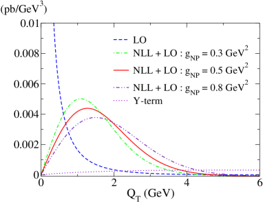
Figure 1: $Q_{T}$ distribution $\Delta_{T}d\sigma/dQ^{2}dQ_{T}dyd\phi$ at $\sqrt{S}=200$ GeV, $Q=8$ GeV, $y=2$ and $\phi=0$.

We would like to thank Werner Vogelsang for providing us with a fortran code of transversity distributions and valuable discussions. We also thank Stefano Catani for fruitful discussions. The work of J.K. and K.T. was supported by the Grant-in-Aid for Scientific Research Nos. C-16540255 and C-16540266.

References

[1]
J.P.Ralston and D.Soper, \NPB152,1979,109.
[2]
G. Bunce, N. Saito, J. Soffer and W. Vogelsang,
Ann.Rev.Nucl.Part.Sci, \andvol50,2000,525.
[3]
W.Vogelsang and A.Weber, \PRD48,1993,2073.
[4]
A.P.Contogouris, B.Kamal and Z.Merebashvili,
\PLB337,1994,167.
[5]
W.Vogelsang, \PRD57,1998,1886.
[6]
G. Altarelli, R. K. Ellis, M. Greco and G. Martinelli,
\NPB246,1984,12.
[7]
J. C. Collins, D. Soper, G. Sterman, \NPB250,1985,199.
[8]
J. Kodaira and L. Trentadue, \PLB112,1982,66;
Report SLAC-Pub-2943 (1982); \PLB123,1983,335.
[9]
A. Hayashigaki, Y. Kanazawa and Y. Koike, \PRD56,1997,7350.
S. Kumano and M. Miyama, \PRD56,1997,2504.
[10]
H. Kawamura et al.,
Nucl. Phys. Proc. Suppl. 135 (2004), 19.
[11]
D. de Florian and M. Grazzini, \PRL85,2000,4678.
[12]
G. Bozzi et al.,
\PLB564,2003,65; hep-ph/0508068.
[13]
E.Laenen, G.Sterman and W.Vogelsang, \PRD63,2001,114018.
S.Kulesza, G.Sterman and W.Vogelsang,
\PRD66,2002,014001.
[14]
S. Catani, M. L. Mangano, P. Nason and L. Trentadue,
\NPB478,1996,273.
[15]
O. Martin et al., \PRD57,1998,3084;
ibid. D 60 (1999), 117502.
[16] A. Kulesza and W. J. Stirling, \JHEP0312,2003,056.
[17]
H. Shimizu, G. Sterman, W. Vogelsang and H. Yokoya, \PRD71,2005,114007.