Distinguishing New Physics Scenarios at a Linear Collider with Polarized Beams

Abstract

Numerous non-standard dynamics are described by contact-like effective interactions that can manifest themselves only through deviations of the cross sections from the Standard Model predictions. If one such deviation were observed, it should be important to definitely identify, to a given confidence level, the actual source among the possible non-standard interactions that in principle can explain it. We here estimate the “identification” reach on different New Physics effective interactions obtainable from angular distributions of lepton pair production processes at the planned International Linear Collider with polarized beams. The models for which we discuss the range in the relevant high mass scales where they can be “identified” as sources of corrections from the Standard Model predictions, are the interactions based on gravity in large and in ${\rm TeV}^{-1}$ extra dimensions and the compositeness-inspired four-fermion contact interactions. The availability of both beams polarized in many cases plays an essential rôle in enhancing the identification sensitivity.

1 Introduction

Numerous new physics (NP) scenarios, candidates as solutions of Standard Model (SM) conceptual problems, are characterized by novel interactions mediated by exchanges of very heavy states with mass scales significantly greater than the electroweak scale. In many cases, theoretical considerations as well as current experimental constraints indicate that the new objects may be too heavy to be directly produced even at the highest energies foreseen at future colliders, such as the CERN Large Hadron Collider (LHC) and the $e^{+}-e^{-}$ International Linear Collider (ILC). In this situation the new, non-standard, interactions could only be revealed by indirect, virtual, effects manifesting themselves as deviations of measured cross sections from the SM predictions.

At the available “low” energies provided by the accelerators, where we study reactions among the familiar SM particles, effective “contact” interaction Lagrangians represent the convenient theoretical tool to physically parameterize the effects of the above mentioned non-standard interactions and, in particular, to test the corresponding virtual high mass exchanges. Clearly, in this framework the transition amplitudes are parameterized as power expansions in the (small) ratios between the Mandelstam variables of the process under study and the high mass scales squared. The sensitivity to the searched for signals will therefore be increased by the colliders high energy (and high luminosity).

Since, in principle, the observation of a correction to the SM cross section may by itself not enable to unambiguously identify its source among the different possible explanations, suitable observables with enhanced sensitivity to the individual non-standard scenarios and/or convenient statistical criteria in the data analysis must be defined in order to discriminate the nature of the relevant new physics model against the others. As regards the search of effective contact interactions at the planned high energy colliders, it should therefore be desirable to assess for each non-standard scenario not only the “discovery reach”, i.e., the maximum value of the relevant mass scale below which it produces observable corrections to the SM predictions, but also the upper limit of the range of mass scale values where the considered scenario not only produces observed deviations, but can also be discriminated from the other potential sources of the deviations themselves. We may call it the “identification reach” of the considered model. Accordingly, it should be important to try to achieve, for the various models, the maximum sensitivity (i.e., discovery reach) as well as highest possible identification reach.

Here, we will try to quantitatively discuss the above issues in the cases of the Kaluza-Klein (KK) graviton exchange in the context of gravity propagating in “large” compactified extra dimensions [?–?], and of the four-fermion contact interactions inspired by the context of leptons and quark compositeness [?–?]. In particular, our aim will be to assess the potential of electron and positron longitudinal polarization at the ILC, to enhance the identification reaches on these NP effective interactions.

Specifically, to this purpose we will take as basic observables the polarized angular differential cross sections of the purely leptonic processes, namely, the Bhabha scattering:

$$e^{+}+e^{-}\to e^{+}+e^{-},$$ (1)

the annihilation into lepton pairs ($l=\mu,\,\tau$):

$$e^{+}+e^{-}\to l^{+}+l^{-},$$ (2)

and the Møller scattering:

$$e^{-}+e^{-}\to e^{-}+e^{-}.$$ (3)

Processes (1)–(3) can all receive contributions from graviton exchange and from four-fermion contact interactions as well, and represent sensitive probes of the above mentioned scenarios, particularly in the case of polarized initial beams [?–?]. Indeed, the interesting feature of the ILC [10] is that polarization of both initial beams can be available [11], and that in principle this collider could be run in both required modes, nemely, $e^{+}e^{-}$ and $e^{-}e^{-}$. In Ref. [12], the identification reach on the different contact interactions was studied by using a Monte Carlo-based analysis of the unpolarized differential cross sections of processes (1) and (2). Electron and positron longitudinal polarization can substantially help in reducing the “confusion” regions of the parameters where models cannot be discriminated from each other on a $\chi^{2}$ basis. Accordingly, the identification reach on the individual models should be enhanced.

In Sec. 2 we give the relevant expressions for the differential polarized angular distributions and for the deviations from the SM predictions in the different NP scenarios considered heres. Secs. 3 and 4 outline the numerical analysis and present the numerical results for the discovery reaches and the distinction among the models, respectively, as allowed by initial beams polarization. Finally, some conclusive remarks are given in Sec. 5.

2 Angular distributions and deviations from the SM

The polarized differential cross section of process (1) can be conveniently written as (see for example [?–?] and [9]):

$$\frac{\mbox{{\rm d}}\sigma(P^{-},P^{+})}{\mbox{{\rm d}}\cos\theta} = \frac{(1+P^{-})\,(1-P^{+})}{4}\,\frac{\mbox{{\rm d}}\sigma_{\rm R}}{\mbox{{\rm d}}\cos\theta}+\frac{(1-P^{-})\,(1+P^{+})}{4}\,\frac{\mbox{{\rm d}}\sigma_{\rm L}}{\mbox{{\rm d}}\cos\theta}$$ (4)

$$+ \frac{(1+P^{-})\,(1+P^{+})}{4}\,\frac{\mbox{{\rm d}}\sigma_{{\rm RL},t}}{\mbox{{\rm d}}\cos\theta}+\frac{(1-P^{-})\,(1-P^{+})}{4}\,\frac{\mbox{{\rm d}}\sigma_{{\rm LR},t}}{\mbox{{\rm d}}\cos\theta},$$

with $\theta$ the angle between incoming and outgoing electrons in the c.m. frame and $P^{\mp}$ the longitudinal polarization of electron and positron beams, respectively. In Eq. (4):

$$\frac{\mbox{{\rm d}}\sigma_{\rm L}}{\mbox{{\rm d}}\cos\theta} = \frac{\mbox{{\rm d}}\sigma_{{\rm LL}}}{\mbox{{\rm d}}\cos\theta}+\frac{\mbox{{\rm d}}\sigma_{{\rm LR},s}}{\mbox{{\rm d}}\cos\theta},$$

$$\frac{\mbox{{\rm d}}\sigma_{\rm R}}{\mbox{{\rm d}}\cos\theta} = \frac{\mbox{{\rm d}}\sigma_{{\rm RR}}}{\mbox{{\rm d}}\cos\theta}+\frac{\mbox{{\rm d}}\sigma_{{\rm RL},s}}{\mbox{{\rm d}}\cos\theta},$$ (5)

where

$$\frac{\mbox{{\rm d}}\sigma_{{\rm LL}}}{\mbox{{\rm d}}\cos\theta} = \frac{2\pi\alpha_{\rm e.m.}^{2}}{s}\,\big{|}G_{{\rm LL},s}+G_{{\rm LL},t}\big{|}^{2},\quad\frac{\mbox{{\rm d}}\sigma_{{\rm RR}}}{\mbox{{\rm d}}\cos\theta}=\frac{2\pi\alpha_{\rm e.m.}^{2}}{s}\,\big{|}G_{{\rm RR},s}+G_{{\rm RR},t}\big{|}^{2},$$

$$\frac{\mbox{{\rm d}}\sigma_{{\rm LR},t}}{\mbox{{\rm d}}\cos\theta} = \frac{\mbox{{\rm d}}\sigma_{{\rm RL},t}}{\mbox{{\rm d}}\cos\theta}=\frac{2\pi\alpha_{\rm e.m.}^{2}}{s}\,\big{|}G_{{\rm LR},t}\big{|}^{2},\quad\frac{\mbox{{\rm d}}\sigma_{{\rm LR},s}}{\mbox{{\rm d}}\cos\theta}=\frac{\mbox{{\rm d}}\sigma_{{\rm RL},s}}{\mbox{{\rm d}}\cos\theta}=\frac{2\pi\alpha_{\rm e.m.}^{2}}{s}\,\big{|}G_{{\rm LR},s}\big{|}^{2}.$$ (6)

The helicity amplitudes $G_{\alpha\beta}$ ($\alpha,\beta={\rm L,R}$) can be expressed in terms of the SM $\gamma$ and $Z$ exchanges in the $s$- and $t$-channels, plus deviations due to contact interactions representing the physics beyond the SM, as follows:

$$G_{{\rm LL},s} = {u}\,\left(\frac{1}{s}+\frac{g_{\rm L}^{2}}{s-M^{2}_{Z}}+\Delta_{{\rm LL},s}\right),\quad G_{{\rm LL},t}={u}\,\left(\frac{1}{t}+\frac{g_{\rm L}^{2}}{t-M^{2}_{Z}}+\Delta_{{\rm LL},t}\right),$$

$$G_{{\rm RR},s} = {u}\,\left(\frac{1}{s}+\frac{g_{\rm R}^{2}}{s-M^{2}_{Z}}+\Delta_{{\rm RR},s}\right),\quad G_{{\rm RR},t}={u}\,\left(\frac{1}{t}+\frac{g_{\rm R}^{2}}{t-M^{2}_{Z}}+\Delta_{{\rm RR},t}\right),$$

$$G_{{\rm LR},s} = {t}\,\left(\frac{1}{s}+\frac{g_{\rm R}\hskip 2.0ptg_{\rm L}}{s-M^{2}_{Z}}+\Delta_{{\rm LR},s}\right),\qquad G_{{\rm LR},t}=s\,\left(\frac{1}{t}+\frac{g_{\rm R}\hskip 2.0ptg_{\rm L}}{t-M^{2}_{Z}}+\Delta_{{\rm LR},t}\right).$$ (7)

Here: $u,t=-s(1\pm\cos\theta)/2$; $M_{Z}$ represents the mass of the $Z$; $g_{\rm R}=\tan\theta_{W}$, $g_{\rm L}=-\cot{2\,\theta_{W}}$ are the SM right- and left-handed electron couplings to the $Z$, with $\theta_{W}$ the electroweak mixing angle.

The advantage of Eqs. (4)–(7) is that the expression for the differential cross section of process (3) can be obtained directly from crossing symmetry: one has to replace $s\leftrightarrow u$, $(P^{-},P^{+})\rightarrow(P^{-}_{1},-P^{-}_{2})$ with $P^{-}_{1}$ and $P^{-}_{2}$ denoting the polarizations of the two initial electrons, and divide the cross section by 2 to account for identical particles. Also, the same equations are easy to adapt to the cross section of the annihilation process (2), one simply must drop all $t$-channel poles (actually, for this process, in principle $\epsilon_{\rm LR}\neq\epsilon_{\rm RL}$ [13]).

Turning to the amplitudes deviations $\Delta_{\alpha\beta}$ in Eq. (7), in the ADD graviton exchange scenario [?–?] only gravity can propagate in two or more extra spatial dimensions of the millimeter order, whereas the SM particles must live only in the ordinary four-dimensional space. Massless graviton exchange in extra dimensions translates to the exchange of a tower of evenly spaced KK massive states (with vertices given in [17, 18], see also [19]), and this effect can be parameterized by the effective, dimension-8, contact interaction Lagrangian [20]

$${\cal L}^{\rm ADD}=i\frac{4\lambda}{\Lambda_{H}^{4}}T^{\mu\nu}T_{\mu\nu}.$$ (8)

Here, $T_{\mu\nu}$ is the energy-momentum tensor of the SM particles, $\Lambda_{H}$ is a ultraviolet cut-off on the summation over the KK spectrum, expected in the (multi) TeV region, and $\lambda=\pm 1$ (models with $\lambda=1$ or $\lambda=-1$ are denoted as ADD+ and ADD$-$, respectively). The explicit expressions of the corresponding corrections to the SM amplitudes relevant to Bhabha scattering are reported in Table 1. In this table, we include also the deviations corresponding to models with ${\rm TeV}^{-1}$-scale extra dimensions, parameterized by the “compactification scale” $M_{C}$, where also the SM gauge bosons may propagate in the additional dimensions [21, 22].

Table 1: Parametrization of the $\Delta_{\alpha\beta}$ functions in different models for $e^{+}e^{-}\to e^{+}e^{-}$

new physics model	$\Delta_{\alpha\beta}$
composite fermions [5]	${\displaystyle{\Delta_{{\alpha\beta},s}=\Delta_{{\alpha\beta},t}=\frac{1}{\alpha_{\rm e.m.}}\frac{\eta_{\alpha\beta}}{\Lambda_{\alpha\beta}^{2}}}}$
${\rm TeV}^{-1}$-scale extra dim. [21, 22]	${\displaystyle{\Delta_{{\alpha\beta},s}=\Delta_{{\alpha\beta},t}=-(Q_{e}Q_{f}+g_{\alpha}^{e}\,g_{\beta}^{f})\,\frac{\pi^{2}}{3\,M_{C}^{2}}}}$
	${\displaystyle{\Delta_{{\rm LL},s}=\Delta_{{\rm RR},s}=\frac{\lambda}{\pi\alpha_{\rm e.m.}\Lambda_{H}^{4}}(u+\frac{3}{4}s)}}$
	${\displaystyle{\Delta_{{\rm LL},t}=\Delta_{{\rm RR},t}=\frac{\lambda}{\pi\alpha_{\rm e.m.}\Lambda_{H}^{4}}(u+\frac{3}{4}t)}}$
ADD model [12, 15]	${\displaystyle{\Delta_{{\rm LR},s}=-\frac{\lambda}{\pi\alpha_{\rm e.m.}\Lambda_{H}^{4}}(t+\frac{3}{4}s)}}$
	${\displaystyle{\Delta_{{\rm LR},t}=-\frac{\lambda}{\pi\alpha_{\rm e.m.}\Lambda_{H}^{4}}(s+\frac{3}{4}t)}}$

Current experimental limits, from LEP2 and Tevatron, are in the range $\Lambda_{H}>1.1-1.3$ TeV [?–?]. For the ${\rm TeV}^{-1}$-scale extra dimension scenario the limit, mostly determined by LEP data, is $M_{C}>6.8\hskip 3.0pt{\rm TeV}$ [27].

The four-fermion contact interaction scenario can be represented by the following vector-vector, dimension-6, effective Lagrangian (with $\eta_{\alpha\beta}=\pm 1,0$ and $\alpha,\beta={\rm L,R}$) [5]:

$${\cal L}^{\rm CI}=\frac{4\pi}{1+\delta_{ef}}\hskip 3.0pt\sum_{\alpha,\beta}\hskip 3.0pt\frac{\eta_{\alpha\beta}}{\Lambda^{2}_{\alpha\beta}}\left(\bar{e}_{\alpha}\gamma_{\mu}e_{\alpha}\right)\left(\bar{f}_{\beta}\gamma^{\mu}f_{\beta}\right),$$ (9)

where $\Lambda_{\alpha\beta}$ denote compositeness scales and $\delta_{ef}=$1 (0) for $f=e$ ($f\neq e$). The most popular four-fermion contact interaction models (CI) are defined by specializing, in Eq. (9), the helicities according to Table 2.

Table 2: Definition of four-fermion CI models

CI model	$\eta_{\rm LL}$	$\eta_{\rm RR}$	$\eta_{\rm LR}$	$\eta_{\rm RL}$
LL	$\pm 1$	0	0	0
RR	0	$\pm 1$	0	0
LR	0	0	$\pm 1$	0
RL	0	0	0	$\pm 1$
VV	$\pm 1$	$\pm 1$	$\pm 1$	$\pm 1$
AA	$\pm 1$	$\pm 1$	$\mp 1$	$\mp 1$

The corresponding deviations $\Delta_{\alpha\beta}$, that appear in Eq. (7), are listed in Table 1. Current limits on $\Lambda$s significantly vary according the process studied and the kind of analysis performed there. In general, the lower bounds are of the order of $10\hskip 2.0pt{\rm TeV}$ (a detailed presentation can be found in the listings of Ref. [28]).

It should be noted from Table 1 that, contrary to the other cases, for the ADD scenario the amplitudes deviations are $z$-dependent ($z\equiv\cos\theta$), and consequently add extra terms, proportional to $z^{3}$ and $z^{4}$, to the SM angular distribution of the annihilation process (2). However, these contributions to the total cross section are expected to be tiny, because the (expected dominant) interference with the SM amplitudes vanishes when integrated over the full angular range and there remain only the terms quadratic in (8), suppressed by the corresponding very high power of the small parameter $1/\Lambda_{H}$. On the contrary, the interference between graviton exchange and $t$-channel SM exchanges for process (1) may give non-vanishing contributions, which may favorably combine with the larger statistical precisions expected in this channel and increase the discovery reach on $\Lambda_{H}$.

3 Discovery reach on the contact interaction models

We here briefly outline the derivation of the expected discovery reaches on the New Physics scenarios introduced in the previous section. The basic objects are the relative deviations of observables from the SM predictions due to the NP:

$$\Delta({\cal O})=\frac{{\cal O}(\rm SM+NP)-{\cal O}(\rm SM)}{{\cal O}(\rm SM)},$$ (10)

and, as anticipated, we concentrate on the differential cross section, ${\cal O}\equiv\mbox{{\rm d}}\sigma/\mbox{{\rm d}}\cos\theta$. To get an illustration of the effects induced by the individual NP models, we show in Figs. 1–3 the angular behavior of the relative deviations (10) for the three leptonic processes under consideration (with unpolarized beams), for c.m. energy $\sqrt{s}=0.5$ TeV and selected values of the relevant mass scale parameters close to their discovery reaches (unpolarized cross sections). The superscript “+” on the CI mass scales $\Lambda_{\alpha\beta}$ denotes the choice $\eta_{\alpha\beta}=1$ in Table 2, while the notation ADD$\pm$ corresponds to $\lambda=\pm 1$ in Eq. (8). Vertical bars represent the statistical uncertainty in each angular bin, for an integrated luminosity ${\cal L}_{\rm int}=100\,{\rm fb}^{-1}$. Of course, the comparison of deviations with statistical uncertainties is an indicator of the sensitivity of an observable to the individual effective interaction models.

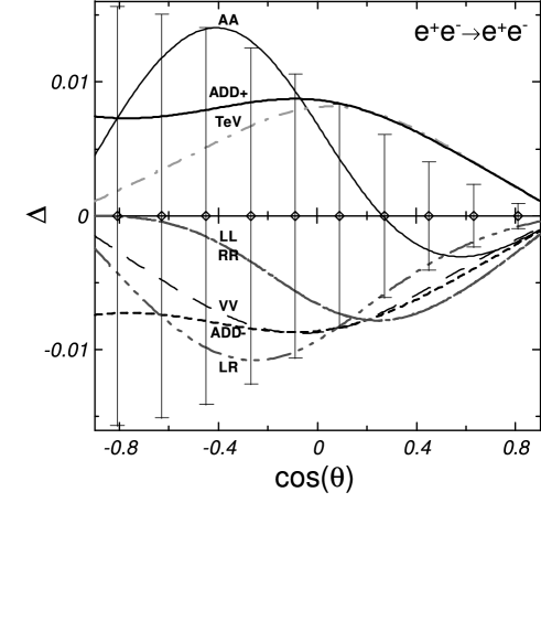
Figure 1: Relative deviations of the unpolarized Bhabha differential cross section from the SM prediction as a function of $\cos\theta$ at $\sqrt{s}=0.5$ TeV for the CI models of Table 2: AA ($\Lambda_{\rm AA}^{+}$=48 TeV), VV ($\Lambda_{\rm VV}^{+}$=76 TeV), LL ($\Lambda_{\rm LL}^{+}$=37 TeV), RR ($\Lambda_{\rm RR}^{+}$=36 TeV), LR ($\Lambda_{\rm LR}^{+}$=60 TeV); for the ${\rm TeV}^{-1}$ model ($M_{C}$=12 TeV) and the ADD$\pm$ models ($\Lambda_{H}$=4 TeV). The vertical bars represent the statistical uncertainty in each bin for ${\cal L}_{\rm int}=100\,{\rm fb}^{-1}$.

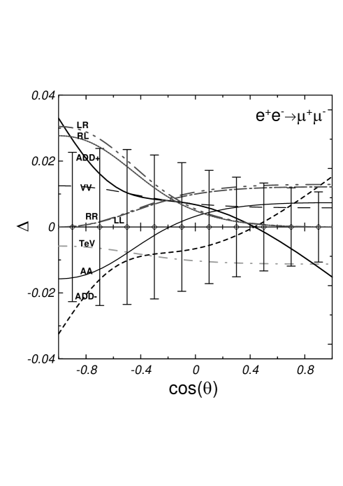
Figure 2: Same as in Fig. 1 but for $e^{+}e^{-}\to\mu^{+}\mu^{-}$, for the CI models of Table 2: AA ($\Lambda_{\rm AA}^{+}$=80 TeV), VV ($\Lambda_{\rm VV}^{+}$=90 TeV), LL ($\Lambda_{\rm LL}^{+}$=45 TeV), RR ($\Lambda_{\rm RR}^{+}$=42 TeV), LR ($\Lambda_{\rm LR}^{+}$=41 TeV), RL ($\Lambda_{\rm RL}^{+}$=43 TeV); for the ${\rm TeV}^{-1}$ model ($M_{C}$=17 TeV) and the ADD$\pm$ models ($\Lambda_{H}$=2.8 TeV).

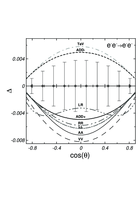
Figure 3: Same as in Fig. 1 but for Møller scattering for the CI models of Table 2: AA ($\Lambda_{\rm AA}^{+}$=55 TeV), VV ($\Lambda_{\rm VV}^{+}$=55 TeV), LL ($\Lambda_{\rm LL}^{+}$=44 TeV), RR ($\Lambda_{\rm RR}^{+}$=44 TeV), LR ($\Lambda_{\rm LR}^{+}$=21 TeV); ${\rm TeV}^{-1}$ model ($M_{C}$=12 TeV) and ADD$\pm$ models ($\Lambda_{H}$=4 TeV). Here, ${\cal L}_{\rm int}(e^{-}e^{-})\approx\frac{1}{3}{\cal L}_{\rm int}(e^{+}e^{-})$ has been assumed.

Basically, a $\chi^{2}$ analysis of the differential cross section of processes (1)–(3) can be performed by dividing the angular range into bins and introducing the sum over bins:

$$\chi^{2}({\cal O})=\sum_{\rm bins}\left(\frac{\Delta({\cal O})^{\rm bin}}{\delta{\cal O}^{\rm bin}}\right)^{2},$$ (11)

where the relative deviations $\Delta({\cal O})$ are defined in Eq. (10) and $\delta{\cal O}$ denotes the expected experimental relative uncertainties, that combine statistical and systematic ones.

As a criterion to constrain the individual models, in particular to set the discovery reach on the relevant mass scales, one essentially looks for the smallest values of such parameters above which the deviation from the SM prediction is too small to be observable within the experimental accuracy. This value, indicated by non-observation of deviations, results from the condition

$$\chi^{2}\leq\chi^{2}_{\rm CL},$$ (12)

where $\chi^{2}_{\rm CL}$ represents a critical value and we will take $\chi^{2}_{\rm CL}=$3.84 for 95% C.L.

To make contact to the foreseeable experimental situation, we impose cuts in the forward and backward directions of processes (1)–(3). Specifically, for Bhabha and Møller scattering we consider the cut angular range $|\cos\theta|<0.9$ and divide it into nine equal-size bins of width $\Delta\cos\theta=0.2$. Similarly, for the annihilation into muon and tau pairs the angular range $|\cos\theta|<0.98$ will be considered. To assess the statistical uncertainty, we assume the reconstruction efficiency $\epsilon=95\%$ for final $l^{+}l^{-}$ events ($l=\mu,\,\tau$), and $\epsilon\simeq 100\%$ for final $e^{+}e^{-}$ and $e^{-}e^{-}$ pairs. Also, to assess the dependence of discovery reaches on the c.m. energy and on the time-integrated luminosity, in the sequel an ILC with $\sqrt{s}=0.5$ TeV and 1 TeV will be considered, with ${\cal L}_{\rm int}(e^{+}e^{-})$ ranging from 100 ${\rm fb}^{-1}$ up to 1000 ${\rm fb}^{-1}$.

Concerning systematic uncertainties, an important source is represented by the uncertainty on beams polarizations, for which we assume $\delta P^{\pm}/P^{\pm}=0.2\%$ (and $\delta P^{-}_{1,2}/P^{-}_{1,2}=0.2\%$ for the case of Møller scattering). Also, a systematic error of 0.5% in the luminosity determination is assumed. In the case of the processes (1) and (3), we analyze the following combinations of beams polarizations: $(P^{-},P^{+})=(|P^{-}|,-|P^{+}|)$; $(-|P^{-}|,|P^{+}|$; $(|P^{-}|,|P^{+}|)$; $(-|P^{-}|,-|P^{+}|)$ with the “standard” envisaged values $|P^{-}|=0.8$ and $|P^{+}|=0.6$ ($|P^{-}_{1}|=|P^{-}_{2}|=0.8$ for Møller scattering). For the annihilation process (2), we limit to the $(P^{-},P^{+})=(|P^{-}|,-|P^{+}|)$ and $(-|P^{-}|,|P^{+}|)$ configurations. As for the time-integrated luminosity, for simplicity we assume it to be equally distributed between the different polarization configurations defined above, and ${\cal L}_{\rm int}(e^{-}e^{-})\approx\frac{1}{3}{\cal L}_{\rm int}(e^{+}e^{-})$ to account for the reduction in luminosity of the $e^{-}e^{-}$ mode due to anti-pinching in the interaction region [29]. The discovery limits are derived by taking the sum of the $\chi^{2}$ relevant to the individual configurations of polarizations mentioned above and imposing the constraint (12). Also, we take into account correlations between the different polarized cross sections, but not those among individual angular bins.

Regarding theoretical inputs, for the SM amplitudes we use the effective Born approximation [30] taking into account electroweak corrections to propagators and vertices, with $m_{\rm top}=175~{}\text{GeV}$ and $m_{\rm H}=120~{}\text{GeV}$. Among the ${\cal O}(\alpha)$ QED corrections, the numerically most important ones come from initial-state radiation. In the case of processes (1) and (2), we account for that effect by a using a structure function approach including both hard and soft photon emission [31] and the flux factor method [32], respectively. To minimize the effect of radiative flux return to the $s$-channel $Z$-exchange, a cut is applied on the radiated photon energy, $\Delta\equiv E_{\gamma}/E_{\rm beam}<1-M_{Z}^{2}/s$ with $\Delta=0.9$, in order that interactions occur close to the nominal collider energy and thus the best sensitivity to the manifestations of non-standard physics can be obtained. Other QED effects, such as final-state and initial-final state emission, are found in process (2) to be numerically unimportant for the chosen kinematical cuts, by using the ZFITTER code [33]. Regarding process (3), the lowest-order corrections to the polarized cross sections are evaluated by means of the FORTRAN code MOLLERAD [?–?], adapted to the present discussion.

The numerical results for the discovery reaches on the effective contact interaction mass scales, obtained by the above procedure in the case of an ILC with $\sqrt{s}=0.5\hskip 3.0pt{\rm TeV}$ and ${\cal L}_{\rm int}(e^{+}e^{-})=100\hskip 3.0pt{\rm fb}^{-1}$, are summarized for the different processes and polarization configurations in Table 3. In this table, only the results for positive interference between SM and non-standard interactions are reported (i.e.,$\eta_{\alpha\beta}=+1$ for CI models and $\lambda=1$ for ADD), because the sensitivity reach for negative interference is practically the same. The results displayed in Table 3 relevant to the processes (1) and (2) with unpolarized beams are consistent with the recent estimates in Ref. [37]. Also, the limits on the CI mass scales resulting from $l^{+}l^{-}$ final states are based on the assumption of $\mu-\tau$ universality.

Table 3: Discovery reach (in TeV) on the mass scale parameters (95% C.L.) from the lepton pair production processes at $\sqrt{s}=0.5$ TeV. For the $e^{+}e^{-}$ mode the three entries refer to ${\cal L}_{\rm int}(e^{+}e^{-})=100\ fb^{-1}$ and the polarizations configurations $(|P^{-}|,|P^{+}|$)=(0,0); (0.8,0); (0.8,0.6). For the $e^{-}e^{-}$ mode the configurations are $(|P_{1}^{-}|,|P_{2}^{-}|)$=(0,0); (0.8,0); (0.8,0.8) and ${\cal L}_{\rm int}(e^{-}e^{-})\approx\frac{1}{3}{\cal L}_{\rm int}(e^{+}e^{-})$.

		process
model		$e^{+}e^{-}\to e^{+}e^{-}$	$e^{-}e^{-}\to e^{-}e^{-}$	$e^{+}e^{-}\to\mu^{+}\mu^{-}$	$e^{+}e^{-}\to l^{+}l^{-}$
ADD$\pm$	($\Lambda_{H}$)	4.1; 4.2; 4.3	3.8; 4.0; 4.1	2.8; 2.8; 2.9	3.0; 3.0; 3.2
VV	($\Lambda$)	76.2; 80.8; 86.4	64.0; 68.8; 71.5	75.5; 76.4; 83.7	89.7; 90.7; 99.4
AA	($\Lambda$)	47.4; 49.1; 69.1	58.0; 62.0; 64.9	67.3; 68.2; 74.8	80.1; 81.1; 88.9
LL	($\Lambda$)	37.3; 45.5; 52.5	43.9; 52.4; 55.2	45.0; 51.0; 57.5	53.4; 60.5; 68.3
RR	($\Lambda$)	36.0; 44.7; 52.2	42.3; 52.3; 55.4	43.2; 50.6; 57.5	51.3; 60.0; 68.3
LR	($\Lambda$)	59.3; 61.6; 69.1	20.1; 22.1; 31.5	40.6; 46.0; 52.6	48.5; 55.0; 62.8
RL	($\Lambda$)	$\Lambda_{RL}=\Lambda_{LR}$	$\Lambda_{RL}=\Lambda_{LR}$	40.8; 46.7; 53.4	48.7; 55.6; 63.6
TeV	($M_{C}$)	12.0; 12.8; 13.8	11.7; 12.5; 12.9	16.8; 17.1; 18.7	20.0; 20.3; 22.2

Some features of the numbers in Table 3 are noteworthy. Firstly, there is complementarity of the leptonic processes under consideration, (1), (2) and (3), in the search for CI and ADD scenarios. Secondly, for the chosen values of the time-integrated luminosity, the discovery reaches on $\Lambda_{H}$ of the Bhabha and Møller scattering processes can be larger than $\simeq 8\sqrt{s}$. Also, Bhabha scattering is the process leading to the best search reach for $\Lambda_{H}$, due to the available higher statistics in the data sample in comparison to either Møller scattering or, to a large extent, to the muon pair production process.

One may recall that, on the purely statistical basis, the discovery reach on $\Lambda_{H}$ should be expected to scale with $s$ and ${\cal L}_{\rm int}$ like $\sim(s^{3}{\cal L}_{\rm int})^{1/8}$, and the discovery reach on the CI mass scales $\Lambda$s like $\sim(s{\cal L}_{\rm int})^{1/4}$, according to the different dimensions of the operators (8) and (9).

4 Distinction among the New Physics models

Let us assume one of the models to be consistent with data and call it “true” model, for example the ADD model (8) with some value of $\Lambda_{H}$. We want to assess the level at which this “true” model is distinguishable from the other ones, that can compete with it as sources of corrections to the SM and we call “tested” models, for any values of the corresponding mass scale parameters. For example, we may take as “tested” model any one of the four-fermion effective contact interactions listed in Table 2. To that purpose, we can introduce relative deviations of the differential cross sections from the ADD predictions in each angular bin, arising from the CI models, analogous to Eq. (10):

$${\tilde{\Delta}}({\cal O})=\frac{{\cal O}({\rm CI})-{\cal O}({\rm ADD})}{{\cal O}({\rm ADD})}.$$ (13)

Correspondingly, a ${\tilde{\chi}}^{2}$ function analogous to Eq. (11) can be introduced, with ${\tilde{\delta}}({\cal O})$ defined in the same way as $\delta({\cal O})$ but, in this case, the statistical uncertainty is referred to the ADD model and therefore depends on the particular value of $\Lambda_{H}$. Since there can be “confusion” regions of $\Lambda_{H}$ and $\Lambda_{\alpha\beta}$ values where also some CI model can be consistent to the ADD predictions, on the basis of such ${\tilde{\chi}}^{2}$ we can study whether these “tested” models can be excluded or not to a given confidence level, that we always assume 95%, once the ADD model has been assumed as “true”. Then, we scan all values of $\Lambda_{H}$ up to the discovery reach.

Thus, let us choose anyone of the “tested” CI models in (13), for definiteness the VV one defined in Table 2, so that the ${\tilde{\chi}}^{2}$ mentioned above will be a function of the two parameters $\epsilon_{\rm CI}\equiv\eta/\Lambda_{\alpha\beta}^{2}$ and $\epsilon_{H}\equiv\lambda/\Lambda_{H}^{4}$ defined in Eqs. (9) and (8), respectively. In Fig. 4, the four gray areas in the ($\epsilon_{\rm CI}$, $\epsilon_{H}$) plane, corresponding to the sign choices ($\eta,\lambda)=(1,1);\,(-1,-1);\,(1,-1);\,(-1,1)$, represent values of the parameters for which both the ADD and the VV models can give observable effects in unpolarized Bhabha scattering at the ILC, with 95% C.L. Also, the horizontal and vertical bands correspond to the discovery reaches on the ADD and VV models at the 95% C.L., derived in the previous section in the unpolarized case. The “confusion region” is the area where the ${\tilde{\chi}}^{2}$ is smaller than $\chi^{2}_{\rm CL}=$3.84 and the two models cannot be distinguished at the 95% C.L.

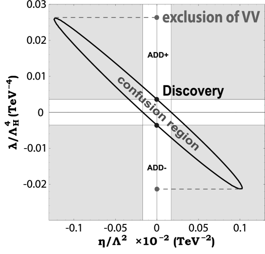
Figure 4: Region of confusion at 95% C.L. for ADD and VV models obtained from unpolarized Bhabha scattering at $\sqrt{s}=$0.5 TeV and ${\cal L}_{\rm int}(e^{+}e^{-})=$100 fb^-1.

As indicated in Fig. 4, one can find a maximal absolute value of the scale parameter $\epsilon_{H}$ for which the “tested” VV model hypothesis is expected to be excluded at the 95% C.L. for any value of the CI parameter $\epsilon_{\rm CI}$ taken in the gray area. We denote the corresponding ADD mass scale parameter as $\Lambda_{H}^{\rm VV}$ and call it “exclusion reach” of the VV model.

It is worth noticing that the “confusion region” is located only in the areas with $(\eta,\lambda)=(1,-1)$ and $(-1,1)$. This is so because in these regions the ADD$\pm$ and VV$\mp$ models provide the same sign of the leading interference with the SM, hence of the deviation in the differential cross sections as depicted in Fig. 1 and, therefore, they can mimic each other. Conversely, there is no confusion region in the areas with $(\eta,\lambda)=(1,1)$ and $(-1,-1)$ where interferences in the angular distribution have opposite signs and therefore can easily be distinguished.

Also, one may point out that, although this kind of $\chi^{2}$ analysis could in principle be applied to any observable, the choice of the differential distribution as basic observable is rather crucial to identify the ADD scenario. Integrated observables such as, for example, the total cross section, the forward-backward asymmetry and the left-right asymmetry, do not allow to derive such a compact confusion region concentrated around the origin as in Fig. 4. For instance, the confusion regions determined from the integrated observables would extend up to a few units of $\lambda/\Lambda_{H}^{4}$ (TeV^-4) and the corresponding reaches on $\Lambda_{H}$ would be too much below the current discovery limits.

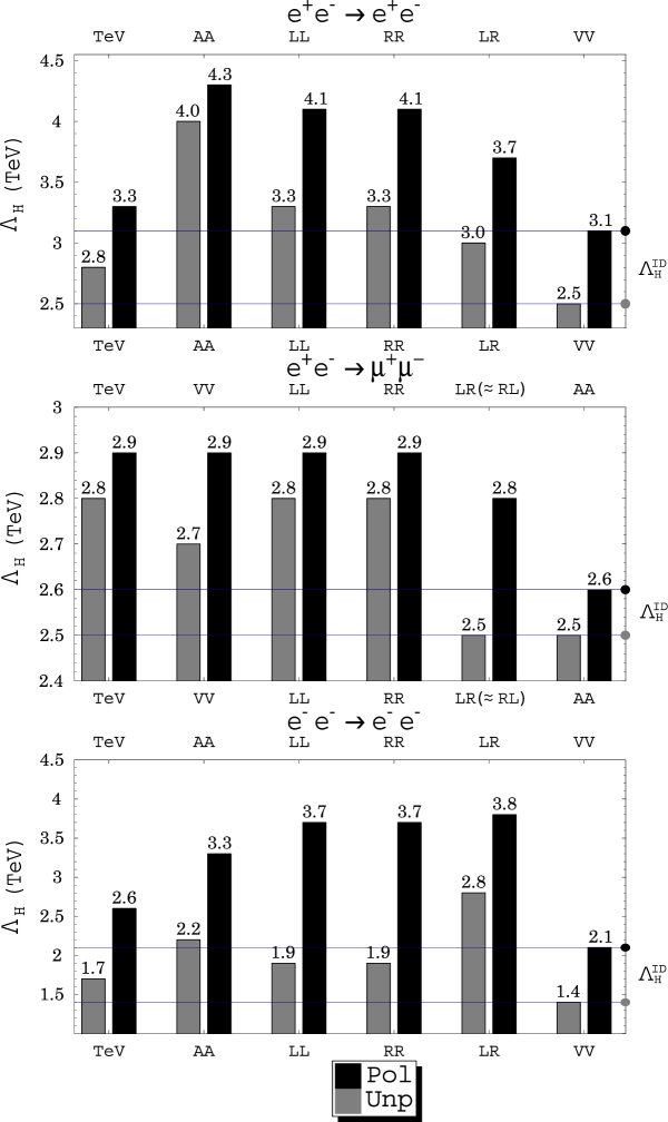
Figure 5: Exclusion and identification reaches on $\Lambda_{H}$ at 95% C.L. obtained from the leptonic processes at $\sqrt{s}=$0.5 TeV, ${\cal L}_{\rm int}(e^{+}e^{-})=$100 fb^-1 for unpolarized beams (gray histograms) and ${\cal L}_{\rm int}(e^{-}e^{-})\approx\frac{1}{3}{\cal L}_{\rm int}(e^{+}e^{-})$ and both beams polarized (black histograms) are illustrated.

The procedure outlined above can be repeated for all other types of effective contact interaction models in Table 2 as well as the ${\rm TeV}^{-1}$ gravity model mentioned in Table 1, and consequently one can evaluate the corresponding “exclusion reaches” $\Lambda_{H}^{\rm AA}$, $\Lambda_{H}^{\rm RR}$, $\Lambda_{H}^{\rm LL}$, $\Lambda_{H}^{\rm LR}$ and $\Lambda_{H}^{\rm TeV}$. The results of this kind of analysis for the three processes of interest here with unpolarized beams (gray histograms) as well as polarized beams (black histograms), are represented in Fig. 5. In this figure, we have considered an ILC with $\sqrt{s}=0.5\hskip 3.0pt{\rm TeV}$, time-integrated luminosity ${\cal L}_{\rm int}(e^{+}e^{-})=100\hskip 3.0pt{\rm fb}^{-1}$ and, in the polarized case, the values of the beams polarizations anticipated in the previous section, i.e.: $|P^{-}|=0.8$ and $|P^{+}|=0.6$ (and for process (3) one third of the $e^{+}e^{-}$ luminosity and $|P_{1}^{-}|=|P_{2}^{-}|=0.8$).

As the final step, the “identification reach” on the ADD scenario can be defined as the minimum of the $\Lambda_{H}$ “exclusion reaches”, $\Lambda_{H}^{\rm ID}=min\{\Lambda_{H}^{\rm VV},\,\Lambda_{H}^{\rm AA},\Lambda_{H}^{\rm RR},\,\Lambda_{H}^{\rm LL},\,\Lambda_{H}^{\rm LR},\,\Lambda_{H}^{\rm TeV}\}$ as indicated in Fig. 5. It is clear that taking $\Lambda_{H}<\Lambda_{H}^{\rm ID}$ allows one to exclude all composite-like CI models as well as the ${\rm TeV}^{-1}$-scale gravity model. In the specific example of the ILC parameters assumed in the derivation of the results of Fig. 5, it turns out that the “identification reach” on the ADD graviton exchange model obtained from unpolarized (polarized) Bhabha scattering corresponds to $\Lambda_{H}^{\rm ID}=$2.5 (3.1) TeV. The identification reaches on $\Lambda_{H}$ obtained from the different leptonic processes are summarized in Table 4.

Table 4: 95% C.L. identification reach on $\Lambda_{H}^{\rm ID}$ at $\sqrt{s}=0.5$ TeV and ${\cal L}_{\rm int}(e^{+}e^{-})=100$ fb^-1.

	$P^{-}=P^{+}=0$	$|P^{-}|=0.8;|P^{+}|=0.6$
process	$\Lambda_{H}^{\rm ID}$ (TeV)	$\Lambda_{H}^{\rm ID}$ (TeV)
$e^{+}e^{-}\to e^{+}e^{-}$	2.5	3.1
$e^{+}e^{-}\to\mu^{+}\mu^{-}$	2.5	2.6
$e^{+}e^{-}\to l^{+}l^{-}$	2.7	2.8
${\cal L}_{\rm int}(e^{-}e^{-})\approx\frac{1}{3}\,{\cal L}_{\rm int}(e^{+}e^{-})$	$P^{-}_{1,2}=0$	$|P^{-}_{1,2}|=0.8$
$e^{-}e^{-}\to e^{-}e^{-}$	1.4	2.1

The rôle of beam polarization in increasing the sensitivity of the leptonic processes to the graviton exchange effects, and particularly in enhancing the potential of distinction from the other NP scenarios, is essential, as exemplified in Fig. 6 in the case of process (1). Indeed, this figure indicates that the reduction of the “confusion region” with respect to the unpolarized case, allowed by beams longitudinal polarization, can be quite substantial.

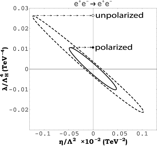
Figure 6: Region of confusion for ADD and VV models obtained from unpolarized (dashed curve) and polarized (solid curve) Bhabha scattering at $\sqrt{s}=$0.5 TeV and ${\cal L}_{\rm int}=$100 fb^-1.

Fig. 7 shows the 95% C.L. identification reach on the graviton exchange mass scale $\Lambda_{H}$ as a function of time-integrated luminosity and two values of the c.m. energy,$\sqrt{s}=$ 0.5 TeV and 1 TeV. The numerical procedure to obtain those results is the $\chi^{2}$ analysis described above, separately applied to the individual processes (1)–(3). In this figure, as well as in the subsequent ones, curves are labelled by the final states of the different processes, i.e., by $e^{+}e^{-}$ for Bhabha scattering, $l^{+}l^{-}$ for the combination of $\mu^{+}\mu^{-}$ and $\tau^{+}\tau^{-}$ production in the annihilation process, and $e^{-}e^{-}$ for Møller scattering. The results for the unpolarized differential cross sections are also shown for comparison. In the case of polarization, the polarized cross sections have been combined similar to the procedure followed in the derivation of the discovery reaches, outlined in the previous section and summarized in Table 3, with the values of longitudinal polarizations exposed there.

The identification reach on the ${\rm TeV}^{-1}$-scale gravity model, obtained by applying the same kind of analysis to the three lepton production processes of interest here, is presented in Fig. 8, while the identification reaches on the four-fermion contact interactions (9) are shown in Figs. 9 and 10. In these figures, curves corresponding to values of identification reaches that are found to fall below the currently available experimental limits (listed in sec. 2) have not been included.

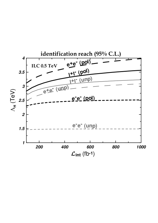
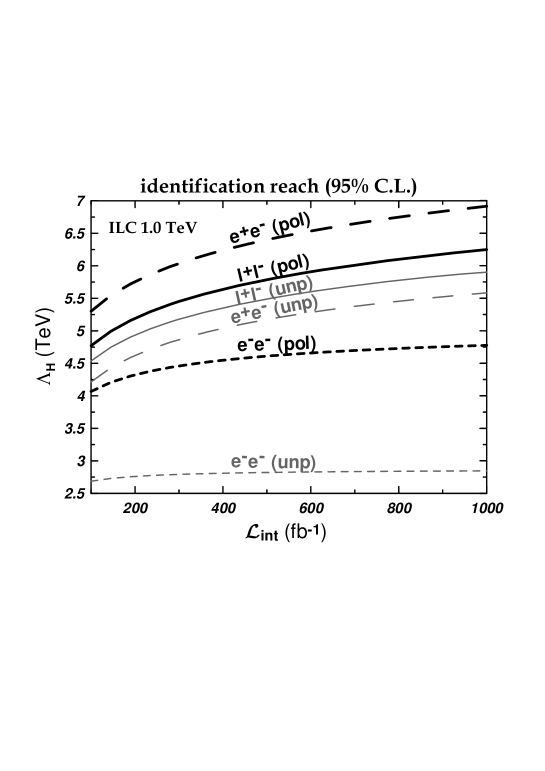
Figure 7: 95% CL identification reach on the cutoff scale $\Lambda_{H}$ in the ADD model as a function of the integrated luminosity obtained from lepton pair production processes with unpolarized and both polarized beams at ILC(0.5 TeV) (left panel) and ILC(1 TeV) (right panel).

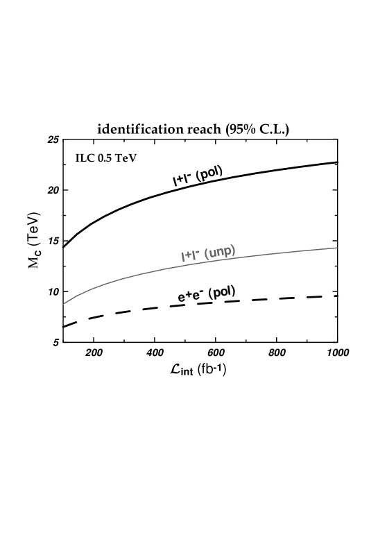
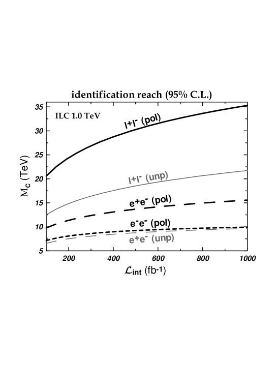
Figure 8: Same as in Fig.7 but for the compactification scale $M_{C}$.

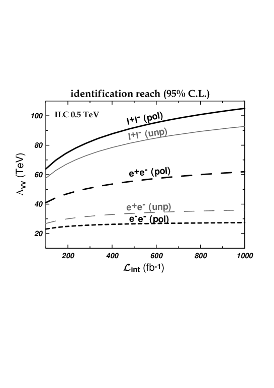
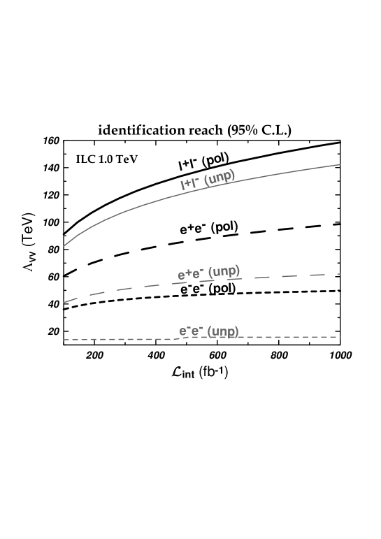
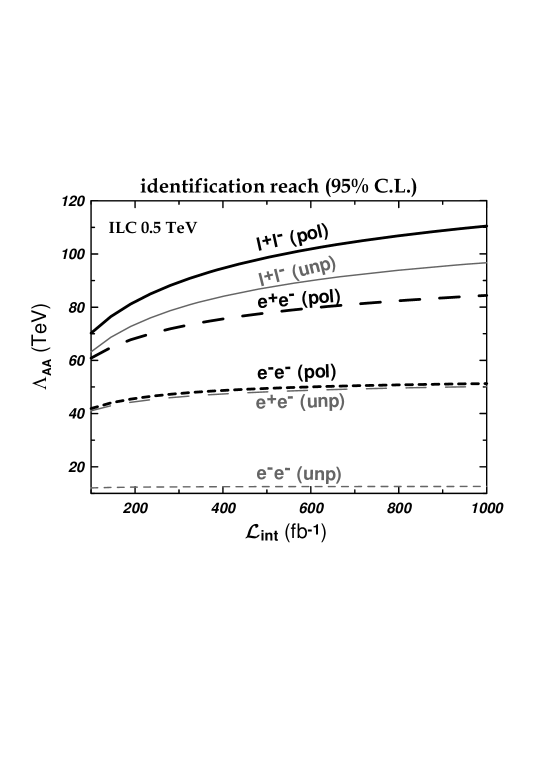
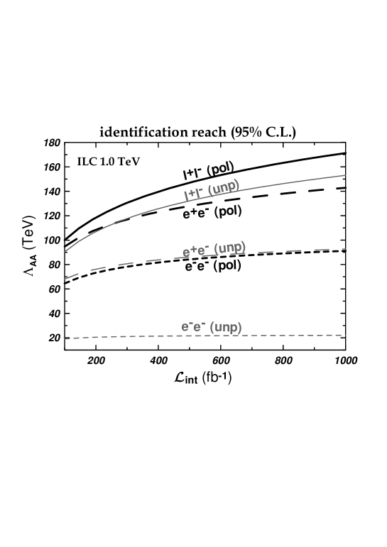
Figure 9: Same as in Fig.7 but for the compositeness scale for $\rm VV$ (top panel), $\rm AA$ (central panel) and $\rm LL$ (lower panel) type interactions.

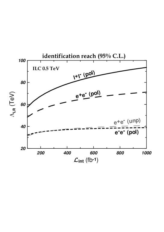
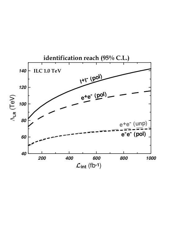
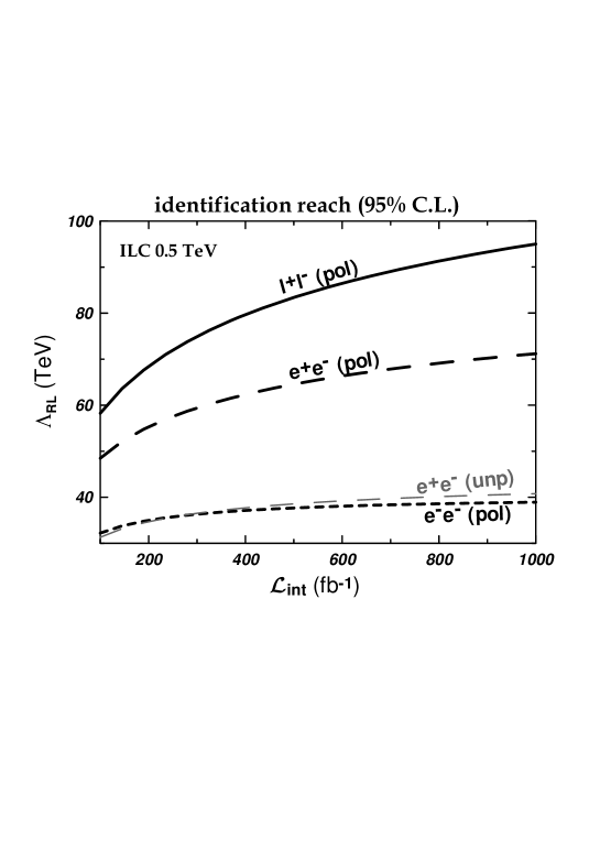
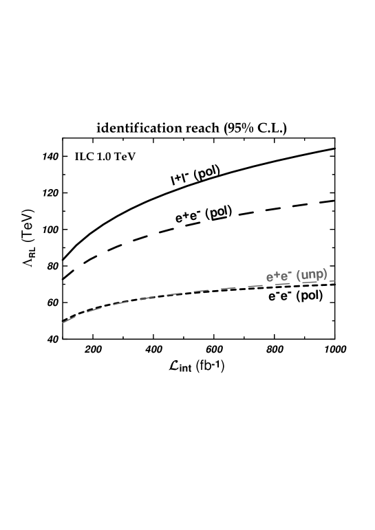
Figure 10: Same as in Fig.7 but for the compositeness scale for $\rm RR$ (top panel), $\rm LR$ (central panel) and $\rm RL$ (lower panel) type interactions.

5 Concluding remarks

We here briefly comment on the main features of the findings in Figs.7–10 for the identification reaches on the effective non-standard interactions considered in Sec. 2, obtainable from lepton pair production at the ILC with longitudinally polarized beams.

Fig. 7 shows that, of the three considered processes, Bhabha scattering definitely has the best identification sensitivity on the scale $\Lambda_{H}$ characterizing the ADD model of Eq. (8) for gravity in “large” compactified extra dimensions. As one can see, in the polarized case, the identification reach ranges from 3.1 TeV to 6.9 TeV, depending on c.m energy and on luminosity. It could be of some interest in this regard to estimate the “resolving power” on $\Lambda_{H}$ obtainable from the polarized process (1). This is defined as the precision that in principle might be achieved on the determination of $\Lambda_{H}$, in the case where the effects of KK graviton exchange were observed. Fig. 11 shows the uncertainty obtainable on $\Lambda_{H}$ when we vary this parameter in the range between the current experimental bound and the expected identification reaches. Of course, the larger $\Lambda_{H}$ the worse the precision on it.

Figure 11: Resolving power $\delta\Lambda_{H}$ on the mass scales ($1\sigma$ level) vs. $\Lambda_{H}$ obtained from the polarized Bhabha scattering for the c.m. energy $\sqrt{s}=$0.5 TeV (left panel) and 1 TeV (right panel) and integrated luminosity of ${\cal L}_{\rm int}=100\hskip 2.0pt{\rm fb}^{-1}$ and $1000\hskip 2.0pt{\rm fb}^{-1}$.

In contrast, although being competitive with the other processes for the discovery reach, Møller scattering is found to give very poor identification reaches on $\Lambda_{H}$ even in the polarized case, and appears to be saturated by the systematic uncertainty as indicated by the corresponding curves quickly becoming flat for increasing luminosity. Indeed, for this for process the KK graviton exchange contribution to the RR and LL cross sections in Eq. (6) is $\cos\theta$-independent therefore identical to the CI interactions (9), while the $\cos\theta$-dependent contribution to the LR cross section is considerably suppressed kinematically. Accordingly, the potential of identification from the angular distributions is reduced. This is qualitatively true in general, i.e., the identification reaches from process (3) are rather moderate, and for some models well-below the discovery reach.

The $l^{+}l^{-}$ annihilation process (2) definitely provides the most stringent identification reaches on ${\rm TeV}^{-1}$-scale gravity in extra dimensions and on the four-fermion contact interactions (9) as well. Quantitatively, Figs. 8–10 show that the identification reach on the compactification mass parameter $M_{C}$ ranges from 15 TeV to 35 TeV depending on the ILC energy and luminosity, and that the reaches on CI four-fermion interactions (9) are rather high and significantly enhanced by polarization: roughly, depending on the energy and the luminosity, the identification reach on $\Lambda_{\rm VV}$ ranges between 62 TeV and 160 TeV; that on $\Lambda_{\rm AA}$ between 70 TeV and 170 TeV; for $\Lambda_{\rm LL}$ between 55 TeV and 135 TeV. Finally, for $\Lambda_{\rm RR}$, $\Lambda_{\rm LR}$ and $\Lambda_{\rm RL}$ the discrimination range can be between 57 TeV and 142 TeV.

As regards the effective rôle of polarization in the derivation of the identification reaches in Figs. 7–10, in particular that of the positron beam polarization in addition to the electron one, it turns out numerically that unpolarized beams do not lead to sensible “identification reaches” on the mass scales relevant to the LL and RR four-fermion CI models in the case of Bhabha and Møller scattering, and on the mass scales of LL, RR, LR, RL models in the case of annihilation into $l^{+}l^{-}$. This relates to the fact that $|g_{\rm L}^{e}|\simeq|g_{\rm R}^{e}|$ so that the (leading) interferences of those NP interactions with the SM have almost identical, hence in practice indistinguishable, angular dependence (see Eq. (7)). Also, unpolarized Møller scattering may give identification limits at the level of current experimental limits, for selected values of energy and luminosity. In general then, for a given process, polarized beams can have much higher identification potential than the unpolarized ones. Specifically, it turns out that the identification reaches in Figs. 7–10 for LL and RR models from Bhabha scattering and those on LL, RR, LR, RL and gravity in ${\rm TeV}^{-1}$ extra dimensions from annihilation into $l^{+}l^{-}$, are mostly rely on electron polarization and not as much on the simultaneous positron polarization. By contrast, the identification reaches on ADD, AA, VV, LR and ${\rm TeV}^{-1}$ models from Bhabha scattering and those on ADD, AA and VV models from annihilation into $l^{+}l^{-}$ pairs definitely need both electron and positron polarization. It may also be noticed that, in many cases, polarized cross sections allow to identify the CI models almost near the discovery reaches (summarized for the lowest considered values of energy and luminosity in Table 3).

Acknowledgements

AAP acknowledges the support of INFN and of MIUR (Italian Ministry of University and research). NP has been partially supported by funds of MIUR and of the University of Trieste. This research has been partially supported by the Abdus Salam ICTP and the World Federation of Scientists (National scholarship programme). AAP and AVT also acknowledge the Belarusian Republican Foundation for Fundamental Research.

References

- [1] N. Arkani-Hamed, S. Dimopoulos and G. R. Dvali, Phys. Lett. B 429, 263 (1998) [arXiv:hep-ph/9803315].
- [2] N. Arkani-Hamed, S. Dimopoulos and G. R. Dvali, Phys. Rev. D 59, 086004 (1999) [arXiv:hep-ph/9807344].
- [3] I. Antoniadis, N. Arkani-Hamed, S. Dimopoulos and G. R. Dvali, Phys. Lett. B 436, 257 (1998) [arXiv:hep-ph/9804398].
-
[4]
G. ’t Hooft, in “Recent Developments In Gauge Theories”, Proceedings,
Nato Advanced Study Institute, Cargese, France, August 26 - September 8, 1979,
edited by
G. ’t Hooft, C. Itzykson, A. Jaffe, H. Lehmann, P. K. Mitter,
I. M. Singer and R. Stora
New York, USA: Plenum (1980)
(Nato Advanced Study Institutes Series: Series B, Physics, 59);
S. Dimopoulos, S. Raby and L. Susskind, Nucl. Phys. B 173, 208 (1980). - [5] E. Eichten, K. D. Lane and M. E. Peskin, Phys. Rev. Lett. 50, 811 (1983).
- [6] R. Rückl, Phys. Lett. B 129, 363 (1983).
- [7] A. A. Pankov and N. Paver, Phys. Rev. D 72, 035012 (2005) [arXiv:hep-ph/0501170].
- [8] P. Osland, A. A. Pankov and N. Paver, Phys. Rev. D 68, 015007 (2003) [arXiv:hep-ph/0304123].
- [9] A. A. Pankov and N. Paver, Eur. Phys. J. C 29, 313 (2003) [arXiv:hep-ph/0209058].
-
[10]
J. A. Aguilar-Saavedra et al. [ECFA/DESY LC Physics Working Group
Collaboration], “TESLA Technical Design Report Part III:
Physics at an Linear Collider,” DESY-01-011, arXiv:hep-ph/0106315;
T. Abe et al. [American Linear Collider Working Group Collaboration], “Linear collider physics resource book for Snowmass 2001. 1: Introduction,” in Proc. of the APS/DPF/DPB Summer Study on the Future of Particle Physics (Snowmass 2001) ed. N. Graf, SLAC-R-570, arXiv:hep-ex/0106055.
K. Abe et al. [ACFA Linear Collider Working Group Collaboration], arXiv:hep-ph/0109166. - [11] G. Moortgat-Pick et al., arXiv:hep-ph/0507011.
- [12] G. Pasztor and M. Perelstein, in Proc. of the APS/DPF/DPB Summer Study on the Future of Particle Physics (Snowmass 2001) ed. N. Graf, arXiv:hep-ph/0111471.
- [13] B. Schrempp, F. Schrempp, N. Wermes and D. Zeppenfeld, Nucl. Phys. B 296, 1 (1988).
- [14] F. Cuypers, eConf C960625, NEW137 (1996) [arXiv:hep-ph/9611336].
- [15] S. Cullen, M. Perelstein and M. E. Peskin, Phys. Rev. D 62, 055012 (2000) [arXiv:hep-ph/0001166].
- [16] B. Qin, U. L. Pen and J. Silk, arXiv:astro-ph/0508572.
- [17] G. F. Giudice, R. Rattazzi and J. D. Wells, Nucl. Phys. B 544, 3 (1999) [arXiv:hep-ph/9811291].
- [18] T. Han, J. D. Lykken and R. J. Zhang, Phys. Rev. D 59, 105006 (1999) [arXiv:hep-ph/9811350].
- [19] G. F. Giudice, T. Plehn and A. Strumia, Nucl. Phys. B 706, 455 (2005) [arXiv:hep-ph/0408320].
- [20] J. L. Hewett, Phys. Rev. Lett. 82, 4765 (1999) [arXiv:hep-ph/9811356].
- [21] K. M. Cheung and G. Landsberg, Phys. Rev. D 65, 076003 (2002) [arXiv:hep-ph/0110346].
- [22] T. G. Rizzo and J. D. Wells, Phys. Rev. D 61, 016007 (2000) [arXiv:hep-ph/9906234].
- [23] S. Ask, arXiv:hep-ex/0410004.
- [24] M. K. Ünel [for the CDF and D0 Collaborations], FERMILAB-CONF-04-206-E, arXiv:hep-ex/0411067.
- [25] G. Landsberg [CDF Collaboration], eConf C040802, MOT006 (2004), [arXiv:hep-ex/0412028].
- [26] V. M. Abazov et al. [D0 Collaboration], Phys. Rev. Lett. 95, 161602 (2005) [arXiv:hep-ex/0506063].
- [27] For a review see, e.g., K. Cheung, arXiv:hep-ph/0409028.
- [28] S. Eidelman et al. [Particle Data Group], Phys. Lett. B 502, 1 (2004).
- [29] J. E. Spencer, Int. J. Mod. Phys. A 11, 1675 (1996).
-
[30]
M. Consoli, W. Hollik and F. Jegerlehner,
CERN-TH-5527-89
Presented at Workshop on Z Physics at LEP;
G. Altarelli, R. Casalbuoni, D. Dominici, F. Feruglio and R. Gatto, Nucl. Phys. B 342, 15 (1990). - [31] For reviews see, e.g., O. Nicrosini and L. Trentadue, in Radiative Corrections for Collisions, ed. J. H. Kühn 25 (Springer, Berlin, 1989), p. 25; in QED Structure Functions, Ann Arbor, MI, 1989, ed. G. Bonvicini, AIP Conf. Proc. No. 201 (AIP, New York, 1990), p. 12.
- [32] For a review see, e.g., W. Benakker and F. A Berends: Proc. of the Workshop on Physics at LEP2, CERN 96-01, vol. 1, p. 79 and references therein.
- [33] D. Bardin, P. Christova, M. Jack, L. Kalinovskaya, A. Olchevski, S. Riemann and T. Riemann, Comput. Phys. Commun. 133, 229 (2001) [hep-ph/9908433].
- [34] V. A. Mosolov, N. M. Shumeiko and J. G. Suarez, Int. J. Mod. Phys. A 15 (2000) 2377.
- [35] N. M. Shumeiko and J. G. Suarez, J. Phys. G 26, 113 (2000) [arXiv:hep-ph/9912228].
- [36] A. Ilyichev and V. Zykunov, Phys. Rev. D 72, 033018 (2005) [arXiv:hep-ph/0504191].
- [37] D. Bourilkov, arXiv:hep-ph/0305125.