Dynamics of quark-gluon plasma from Field correlators

Abstract

It is argued that strong dynamics in the quark-gluon plasma and bound states of quarks and gluons is mostly due to nonperturbative effects described by field correlators. The emphasis in the paper is made on two explicit calculations of these effects from the first principles – one analytic using gluelump Green’s functions and another using independent lattice data on correlators. The resulting hadron spectra are investigated in the range $T_{c}\leq T<2T_{c}$. The spectra of charmonia, bottomonia, light $s\bar{s}$ mesons, glueballs and quark-gluon states calculated numerically are in general agreement with lattice MEM data. The possible role of these bound states in the thermodynamics of quark-gluon plasma is discussed.

1 Introduction

The importance of nonperturbative dynamics in QCD, which is illustrated by the phenomena of confinement and chiral symmetry breaking, was also proposed some time ago for the deconfined phase [1] – [3]. In the framework of the Vacuum Correlator Method (VCM) (sometimes also called Stochastic Vacuum Model) [4] it was shown (see [5] for a review), that four dominant correlators of the QCD vacuum $D^{(E,H)}(x)$, $D_{1}^{(E,H)}(x)$ define with few percent accuracy all dynamics of the QCD vacuum and hadrons both below and above $T_{c}$, and $D^{(E)}(x)$ is responsible for confinement, with the string tension $\sigma^{(E)}=1/2\int D^{(E)}(x)d^{2}x$. Above $T_{c}$ as was predicted in [1] – [3], $D^{E}(x)$ vanishes, while $D_{1}^{(E)}(x)$ stays nonzero and may support the nonperturbative dynamics at $T\geq T_{c}$ (together with magnetic corrections due to $D^{(H)}(x),D_{1}^{(H)}(x)$).

At approximately the same time, starting from 1992, a careful study of field correlators was performed by the Pisa group [6, 7] resulting in the explicit forms of four independent field correlators $D^{(E)},D_{1}^{(E)},D^{(H)}$ and $D_{1}^{(H)}$ both below and above $T_{c}$. It was concluded from these results that indeed $D^{(E)}$ vanishes at $T\geq T_{c}$, while three other correlators stay nonzero at least till $T=1.26T_{c}$.

It was suggested in [1] that $D_{1}^{(E)}(x)$ is responsible for possible bound states of quarks and gluons in the quark-gluon plasma, which was then called “the strong interacting quark-gluon plasma”. Recently this phenomenon was observed in the lattice at $T\geq T_{c}$ in the form of bound states of light $q\bar{q}$ mesons [8], heavy quarkonia $(c\bar{c})$ [9] – [13] and three-quark stetes [14]. Moreover, the thermodynamic quantities associated with the $Q\bar{Q}$ system, namely free energy $F^{(Q\bar{Q})}(r,T)$ and internal energy $U^{(Q\bar{Q})}(r,T)$ have been measured [13, 15, 16] for the $Q\bar{Q}$ distance $r$ in the interval $0\leq r\mathrel{\mathchoice{\lower 3.6pt\vbox{\halign{$\mathsurround=0pt\displaystyle\hfil#\hfil$\cr<\crcr\sim\crcr}}}{\lower 3.6pt\vbox{\halign{$\mathsurround=0pt\textstyle\hfil#\hfil$\cr<\crcr\sim\crcr}}}{\lower 3.6pt\vbox{\halign{$\mathsurround=0pt\scriptstyle\hfil#\hfil$\cr<\crcr\sim\crcr}}}{\lower 3.6pt\vbox{\halign{$\mathsurround=0pt\scriptscriptstyle\hfil#\hfil$\cr<\crcr\sim\crcr}}}}2$ fm, showing large asymptotic value, e.g. $F(\infty,T_{c})\approx 600$ MeV for $n_{f}=2$ [16].

These latter quantities can be explained only by nonperturbative effects, since perturbative OGE potential, even with increased $\alpha_{S}(r)$, cannot produce similar effect.

At the same time, it is characteristic for the static potential $V_{1}(r,T)$ produced by the correlator $D_{1}^{E}(x)$, that it indeed gives rise to the constant term $V_{1}(\infty,T)$ in the $Q\bar{Q}$ interaction at large distances, which can be viewed upon as the sum of constant selfenergies of $Q$ and $\bar{Q}$.

It was argued in the recent paper [17] by one of the authors (Yu.S.), that this strong interaction observed in the quark-gluon plasma on the lattice in [8] – [16], and possibly seen in the ion-ion collisions at RHIC [18], can be explained by the correlator $D_{1}^{E}(x)$. To check this prediction in [17] the analytic form of $D_{1}^{E}(x)$ was used calculated before in [19], exploiting the connection of field correlators to the gluelump Green’s functions. In this way the static $Q\bar{Q}$ potential $V_{1}(r,T)$ was computed from $D_{1}^{E}(x)$ and compared to the lattice free energy $F^{(Q\bar{Q})}(r,T)$. The resulting agreement has demonstrated that the $D_{1}^{(E)}(x)$ can be considered as a calculable source of strong interaction above $T_{c}$.

Based on $V_{1}(r,T)$ the possibility of bound states of heavy quarkonia, glueballs and baryons was established, using the Bargmann condition for the static potential.

It is a purpose of the present paper to calculate explicitly the possible bound states of quarks and gluons using directly the previously calculated $D_{1}^{(E)}(x)$ on the lattice as an input. In doing so a new fit of lattice data is done, using the analytically calculated form of $D_{1}^{(E)}(x)$, found in [6, 7]. For comparison we also use static potential obtained from the analytic expression of $D_{1}^{(E)}$, found in [19] for $T\leq T_{c}$ and analytically continued to $T\geq T_{c}$.

With the help of these sets of static potential, lattice and analytic, $V_{1}^{(\rm lat)}$ and $V_{1}^{(\rm anal)}$, we calculate the bound states of charmonia, bottomonia, strange quarkonia and glueballs and compare it with existing lattice data.

Having calculated possible bound states, we discuss their possible role in the thermodynamics, and in particular, the effective masses of quarks and gluons and the contribution to the free and internal energy with the aim to explain the difference $(\varepsilon-3p)$ above $T_{c}$ and ratio $\varepsilon/\varepsilon_{SB}$.

The paper is organized as follows. In the next section we introduce the analytic gluelump expression for $D_{1}^{(E)}$ and the static potential derived from it. In section 3 the analytic form of $D_{1}^{(E)}$ is tested with existing lattice data in the interval $1.007T_{c}\leq T\leq 1.26T_{c}$ and in section 4 the static potential is derived from the lattice data. In section 5 we write the Hamiltonian for heavy and light quarkonia, glueballs and quark-gluon states. In section 6 numerical results for bound states in concrete systems are considered and discussed in comparison to lattice data. The possible role of calculated objects in the thermodynamics of quark-gluon plasma is envisaged, and the suppression factor for the colored states is derived.

2 Analytic form of field correlators and the $Q\bar{Q}$ static potential at $T=0$

We start with the standard definitions of the field correlator functions $D(x)$ and $D_{1}(x)$, defined as in [4], which are measured in [6, 7]

$$\frac{g^{2}}{N_{c}}\langle tr_{f}(F_{\mu\nu}(x)\Phi(x,y)F_{\lambda\sigma}(y)\Phi(y,x))\rangle\equiv D_{\mu\nu,\lambda\sigma}(x,y)=$$

$$=(\delta_{\mu\lambda}\delta_{\nu\sigma}-\delta_{\mu\sigma}\delta_{\nu\lambda})D(x-y)+\frac{1}{2}\left(\frac{\partial}{\partial x_{\mu}}h_{\lambda}\delta_{\nu\sigma}+perm.\right)D_{1}(x-y)$$ (1)

where $h_{\mu}=x_{\mu}-y_{\mu},~{}~{}\Phi(x,y)=P\exp ig\int^{x}_{y}A_{\mu}dz_{\mu}$ and $tr_{f}$ is the trace in the fundamental representation. Our final aim in this section will be to connect $D(x),D_{1}(x)$ to the gluelump Green’s functions. These Green’s functions are however not accessible for direct analytic calculation and to proceed one needs to use Background Field Formalism (BFF) [20], where the notions of valence gluon field $a_{\mu}$ and background field $B_{\mu}$ are introduced, so that total gluonic field $A_{\mu}$ is written as

$$A_{\mu}=B_{\mu}+a_{\mu}$$ (2)

Using (2) one can write the total field operator $F_{\mu\nu}(x)$ as follows

$$F_{\mu\nu}(x)=\partial_{\mu}A_{\nu}-\partial_{\nu}A_{\mu}-ig[A_{\mu},A_{\nu}]=$$

$$=\partial_{\mu}(a_{\nu}+B_{\nu})-\partial_{\nu}(a_{\mu}+B_{\mu})-ig[a_{\mu}+B_{\mu},a_{\nu}+B_{\nu}]=$$ (3)

$$=\hat{D}_{\mu}a_{\nu}-\hat{D}_{\nu}a_{\mu}-ig[a_{\mu},a_{\nu}]+F^{(B)}_{\mu\nu}.$$

Here the term, $F_{\mu\nu}^{(B)}$ contains only the field $B_{\mu}^{b}$. To proceed one can use the idea [21] of the background field $B_{\mu}^{(b)}$ as the collective field of all gluons with color indices $b$, with $b$ occupying most of indices from 1 to $N_{c}^{2}-1$, while the color index $"a"$ of $a_{\mu}^{a}$ having only few values. The physical idea, realized in [19, 21] is that after averaging over all fields $B_{\mu}^{(b)}$ in the vacuum, the resulting interaction for the valence gluon is diagonal in index $"a"$ and has the form of the white adjoint string. It is clear that when one averages over field $a_{\mu}^{a}$ and sums finally over all color indices $a$, one actually exploits all the fields with color indices from $F^{(B)}_{\mu\nu}$, so that the term $F_{\mu\nu}^{(B)}$ can be omitted, if summing over all $a$ is presumed to be done at the end of calculation. In this section we shall concentrate on the first two terms on the r.h.s. of (3), which yield $D_{1}(x)$.

Assuming the background Feynman gauge, $D_{\mu}a_{\mu}=0,$ we shall define now the gluelump Green’s function as

$$G_{\mu\nu}(x,y)=\langle tr_{a}a_{\mu}(x)\hat{\Phi}(x,y)a_{\nu}(y)\rangle.$$ (4)

We    can   also    write   for   the   gluelump   Green’s    function     (4))
$G_{\mu\nu}(x,y)=\delta_{\mu\nu}f((x-y)^{2})$ in the limit of vanishing gluon spin-dependent interaction, see discussion below.

As a result one obtains from (3,4) the following connection of $D^{(0)}$ and $f((x-y)^{2})$ (see [19] for details of derivation)

$$D^{(0)}_{4i,4k}(x,y)=\frac{g^{2}}{2N_{c}^{2}}\left\{\frac{\partial}{\partial x_{4}}\frac{\partial}{\partial y_{4}}\delta_{ik}f((x-y)^{2})+\frac{\partial}{\partial x_{i}}\frac{\partial}{\partial y_{k}}f((x-y)^{2})\right\},$$ (5)

on the other hand using (1) with $h_{\mu}\equiv x_{\mu}-y_{\mu}$ one can express $D^{(0)}_{4i,4k}$ through $D_{1}$ as

$$D_{4i,4k}^{(0)}(h)=\delta_{ik}D(h)+\frac{1}{2}\left(\frac{\partial}{\partial x_{4}}h_{4}D_{1}\delta_{ik}+\frac{\partial}{\partial x_{i}}h_{k}D_{1}\right)$$ (6)

and for $h_{i}=0,i=1,2,3,h_{4}\neq 0$ one obtains

$$D_{1}(x)=-\frac{2g^{2}}{N^{2}_{c}}\frac{df(x^{2})}{dx^{2}},~{}~{}G_{\mu\nu}(x,y)=\delta_{\mu\nu}f((x-y)^{2})$$ (7)

To obtain information about the gluelump Green’s function $G_{\mu\nu}$ one can use the path-integral representation of $G_{\mu\nu}(x,y)$ in the Fock-Feynman-Schwinger (FFS) formalism (see [22] for reviews and original references), which was exploited for gluelump Green’s function in [23]

$$G_{\mu\nu}(x,y)=tr_{a}\int^{\infty}_{0}ds(Dz)_{xy}e^{-K}\langle W^{(F)}_{\mu\nu}(C_{xy})\rangle$$ (8)

where $K=\frac{1}{4}\int^{s}_{0}\left(\frac{dz_{\mu}}{d\tau}\right)^{2}d\tau$ and

$$W^{F}_{\mu\nu}(C_{xy})=PP_{F}\left\{\exp(ig\int A_{\lambda}dz_{\lambda})\exp(2ig\int^{s}_{0}d\tau\hat{F}_{\sigma\rho}(z(\tau)))\right\}_{\mu\nu}$$ (9)

and the closed contour $C_{xy}$ is formed by the straight line from $y$ to $x$ due to the heavy adjoint source Green’s function and the path of the valence gluon $a_{\mu}$ from $x$ to $y$. Note that the nontrivial $\{\mu\nu\}$ dependence of the r.h.s. of (9) occurs only due to the $\hat{F}_{\nu\rho}$; expanding in powers of this term, one has $W_{\mu\nu}^{F}=W^{(0)}\delta_{\mu\nu}+W^{(1)}\hat{F}_{\mu\nu}+...$ In what follows we shall neglect $W^{(n)}$ with $n\geq 1$ since these terms correspond to the effect of spin-dependent forces in gluelump, which are relatively small and were accounted for in [23].

Neglecting in $G_{\mu\nu}$ gluon fields altogether we obtain the perturbative result, $G_{\mu\nu}\to G^{(0)}_{\mu\nu}$

$$G_{\mu\nu}^{(0)}(x,y)=\frac{N_{c}(N^{2}_{c}-1)\delta_{\mu\nu}}{4\pi^{2}(x-y)^{2}}.$$ (10)

This is the leading term in the expansion of $G_{\mu\nu}$ at small $|x-y|$, while the next order term is found in [19] to be

$$D_{1}(x)=\frac{4C_{2}\alpha_{s}}{\pi}\left\{\frac{1}{x^{4}}+\frac{\pi^{2}G_{2}}{24N_{c}}+...\right\},$$ (11)

where $G_{2}$ is the standard gluonic condensate [24]

$$D(0)+D_{1}(0)=\frac{g^{2}}{12N_{c}}trF^{2}(0)=\frac{\pi^{2}}{18}G_{2}.$$ (12)

One can prove consistency of the resulting $D_{1}(x)$ as follows.

Checking constant term in (11), one can compare $D_{1}(0)$ on the l.h.s. of (11) with the r.h.s., $D_{1}(0)=\frac{\alpha_{s}C_{2}}{\pi}\cdot\frac{\pi^{2}}{18}G_{2}=\frac{\alpha_{s}C_{2}}{\pi}(D(0)+D_{1}(0))$, where $D(0)+D_{1}(0)$ on the r.h.s. of (11) are defined by the gluon condensate, Eq. (12). Since $\frac{\alpha_{s}C_{2}}{\pi}\mathrel{\mathchoice{\lower 3.6pt\vbox{\halign{$\mathsurround=0pt\displaystyle\hfil#\hfil$\cr<\crcr\sim\crcr}}}{\lower 3.6pt\vbox{\halign{$\mathsurround=0pt\textstyle\hfil#\hfil$\cr<\crcr\sim\crcr}}}{\lower 3.6pt\vbox{\halign{$\mathsurround=0pt\scriptstyle\hfil#\hfil$\cr<\crcr\sim\crcr}}}{\lower 3.6pt\vbox{\halign{$\mathsurround=0pt\scriptscriptstyle\hfil#\hfil$\cr<\crcr\sim\crcr}}}}1$, this estimate of $D_{1}(0)$ is reasonable and suggests that for $\alpha_{s}=0.4$ the magnitude of $D_{1}(0)$ is 0.2 $D(0)$.

This ratio is in agreement with the lattice calculations in [6].

In another check one considers the singular term, $D_{1}^{sing}(x)=\frac{4C_{2}\alpha_{s}}{\pi x^{4}}$ and inserts it in the static $Q\bar{Q}$ potential. The static $Q\bar{Q}$ potential can be expressed through $D$ and $D_{1}$, as was done in [25]:

$$V(r) = 2r\int^{r}_{0}d\lambda\int^{\infty}_{0}d\nu D(\lambda,\nu)+\int^{r}_{0}\lambda d\lambda\int^{\infty}_{0}d\nu[-2D(\lambda,\nu)+D_{1}(\lambda,\nu)]$$ (13)

$$\equiv V_{D}(r)+V_{1}(r).$$

Inserting in (13) the perturbative part of $D_{1}$ from (11) one obtains the standard color Coulomb potential $V_{C}(r)=-\frac{4\alpha_{s}}{3r}$, thus checking the correct normalization of $D_{1}(x)$.

Another form of $G_{ik}(x,y)$ is available at all distances and practically important at large $|x-y|$, namely

$$G_{ik}(x,y)=N_{c}(N^{2}_{c}-1)\sum^{\infty}_{n=0}\Psi^{(i)}_{n}(0)\Psi^{(k)^{+}}_{n}(0)e^{-M_{n}|x-y|}$$ (14)

where $\Psi_{n}^{(i)}(x),M_{n}$ are eigenfunction and eigenvalue of the gluelump Hamiltonian, [23], details are given in Appendices 1,2,3,4 of ref. [19].

For $\Psi_{n}^{(\mu)}(0)$ one can use the known equation, which is obtained from the eigenfunctions $\Psi_{n}$ of $H_{0}$ through the connection

$$\Psi^{(\mu)}_{n}=\frac{e_{\mu}}{\sqrt{2\mu}}\psi_{n},~{}~{}\left(\Psi_{n}^{(\mu)}(0)\right)^{2}=\frac{\sigma_{adj}}{4\pi}.$$ (15)

Inserting (15) into (14) one obtains

$$G_{\mu\nu}(x,y)\approx N_{c}(N^{2}_{c}-1)\sum^{\infty}_{n=0}\delta_{\mu\nu}\frac{(\sigma_{adj})}{4\pi}e^{-M_{n}|x-y|}.$$ (16)

It is clear that for $x\to y$ the sum in (16) diverges and one should use instead of (16) the perturbative answer (10). For large $|x-y|$ one can keep in (16) only the terms with the lowest mass, i.e. for the color electric gluelump state $1^{--}$, which obtains for spacial $\mu,\nu=i,k$

Thus one gets

$$G_{ik}\left|{}_{|x-y|\to\infty}\right.\approx(N^{2}_{c}-1)\frac{N_{c}\sigma_{adj}}{4\pi}\delta_{ik}e^{-M_{0}|x-y|}.$$ (17)

The eigenvalue $M_{0}$ was found in [23] to be $M_{0}\cong(1.49\div 0.98)$ GeV for $\sigma_{f}=0.18$ GeV² and $\bar{\alpha}_{s}=(0\div 0.195)$. This should be compared with the value $M_{0}=1.5\pm 0.4$ GeV, obtained from the QCD sum rules in [26] and with the lattice value $M_{0}\approx 1$ GeV obtained in [6, 7] from asymptotic of $D_{1}$.

Using (7) one can define from (17) the nonperturbative part of $D_{1}$, which is valid at large $|x|$,

$$D_{1}^{(nonp)}(x)=\frac{C_{2}(f)\alpha_{s}2M_{0}\sigma_{adj}}{\sqrt{x^{2}}}e^{-M_{0}|x|},~{}~{}C_{2}(f)=\frac{N^{2}_{c}-1}{2N_{c}}$$ (18)

and the total $D_{1}$ due to (7) and (10) can be represented as

$$D_{1}(x)=\frac{4C_{2}(f)\alpha_{s}}{\pi x^{4}}e^{-\gamma|x|}+D_{1}^{(nonp)}(x)$$ (19)

and $\gamma$ plays the role of screening length of gluon.

One can easily see that insertion of (7) into $V_{1}(R)$ allows to express $V_{1}(R)$ in terms of $f(x)$,

$$V_{1}(R)=-\frac{g^{2}}{N_{c}^{2}}\int^{\infty}_{0}d\nu(f(R^{2}+\nu^{2})-f(\nu^{2})).$$ (20)

For the purely perturbative $f(x^{2})$,

$$f=f^{(0)}(x^{2})=\frac{N_{c}(N_{c}^{2}-1)}{4\pi^{2}x^{2}}$$ (21)

one has from (20) the standard lowest order Coulomb interaction

$$V_{1}(R)=-\frac{C_{2}(f)\alpha_{s}}{R}.$$ (22)

Note that the last term in this case, $V_{1}(\infty)\equiv\frac{g^{2}}{N^{2}_{c}}\int^{\infty}_{0}f(\nu^{2})d\nu$ is diverging at small $\nu$, which is connected to the well-known perimeter divergence of fixed-contour Wilson or Polyakov lines, which is renormalized on the lattice [12, 16], subtracting short-distance part of potential at $T=0$. In what follows we shall concentrate on the nonperturbative part of $V_{1}(R)$ representing it as $V_{1}(R)=V_{1}^{(pert)}(R)+V_{1}^{(np)}(R)$, where $V_{1}^{pert}$ can be treated as the screened Coulomb potential, so that renormalization of the Wilson (Polyakov) lines would affect only $V_{1}^{pert}(R)$.

One can easily see in (20) that $V_{1}(\infty)$ is actually the sum of self-energy parts of quark and antiquark, occurring due to the gluelump exchange with time interval $\nu$.

3 Analytic form $vs$ lattice data at $T>T_{c}$

A detailed study by numerical simulations on a lattice of the behaviour of the gauge–invariant two–point correlation functions of the gauge–field strengths across the deconfinement phase transition ($T\sim T_{c}$), both for the pure–gauge $SU(3)$ theory and for full QCD with two flavours, has been performed in Ref. [27]. Quenched data published in [27] agree within errors with previous determinations [28] (obtained on a $16^{3}\times 4$ lattice, in a range of distances from $0.4$ to 1 fm approximately) but have been obtained on a larger lattice ($32^{3}\times 6$) and with much higher statistics.

For the benefit of the reader (and essentially for defining the notations used in the rest of the paper) we report here some technical details about the lattice determination of the correlators in [27]. To simulate the system at finite temperature, a lattice is used of spatial extent $N_{\sigma}\gg N_{\tau}$, $N_{\tau}$ being the temporal extent, with periodic boundary conditions for gluons and antiperiodic boundary conditions for fermions in the temporal direction. The temperature $T$ corresponding to a given value of $\beta=2N_{c}/g^{2}$ is given by

$$N_{\tau}\cdot a={1\over T}~{},$$ (23)

where $a$ is the lattice spacing. In the quenched case $a$ only depends on the coupling $\beta$ and, from renormalization group arguments,

$$a(\beta)={1\over\Lambda_{L}}f(\beta)~{},$$ (24)

where $f(\beta)$ is the so–called scaling function and $\Lambda_{L}$ is the scale parameter of QCD in the lattice regularization scheme. At large enough $\beta$, $f(\beta)$ is given by the usual two–loop expression:

$$f(\beta)=\left({8\over 33}\,\pi^{2}\beta\right)^{51/121}\exp\left(-{4\over 33}\pi^{2}\beta\right)\left[1+{\cal O}(1/\beta)\right]~{},$$ (25)

for gauge group $SU(3)$ and in the absence of quarks. The expression (25) can also be used in a small enough interval of $\beta$’s lower than the asymptotic scaling region, and then $\Lambda_{L}$ is an effective scale depending on the position of the interval considered. The lattice used in Ref. [27] for the quenched case was a $32^{3}\times 6$ (in our notation, $N_{\sigma}=32$ and $N_{\tau}=6$) and the critical temperature $T_{c}$ for such a lattice corresponds to $\beta_{c}\simeq 5.8938$ [29]. The range of values of $\beta$’s considered in Ref. [27] goes from $\beta=5.85$ to $\beta=6.10$ and in this interval the effective scale $\Lambda_{L}$ is about 4.9 MeV.

At finite temperature ($N_{\sigma}\gg N_{\tau}$) the $O(4)$ space–time symmetry is broken down to the spatial $O(3)$ symmetry and the bilocal correlators are expressed in terms of five independent functions [1]-[3], [6, 7]. Two of them are needed to describe the electric–electric correlations:

$${g^{2}\over N_{c}}\langle tr_{f}[E_{i}(x)\Phi(x,y)E_{k}(y)\Phi(y,x)]\rangle$$ (26)

$$=\delta_{ik}\left[{D}^{E}+{D}_{1}^{E}+u_{4}^{2}{\partial{D}_{1}^{E}\over\partial u_{4}^{2}}\right]+u_{i}u_{k}{\partial{D}_{1}^{E}\over\partial\vec{u}^{2}}~{},$$

where $E_{i}=F_{i4}$ is the electric field operator and $u_{\mu}=x_{\mu}-y_{\mu}$, [$\vec{u}^{2}=(\vec{x}-\vec{y})^{2}$].

Two further functions are needed for the magnetic–magnetic correlations:

$${g^{2}\over N_{c}}\langle tr_{f}[H_{i}(x)\Phi(x,y)H_{k}(y)\Phi(y,x)]\rangle$$ (27)

$$=\delta_{ik}\left[{D}^{H}+{D}_{1}^{H}+\vec{u}^{2}{\partial{D}_{1}^{H}\over\partial\vec{u}^{2}}\right]-u_{i}u_{k}{\partial{D}_{1}^{H}\over\partial\vec{u}^{2}}~{},$$

where $H_{k}={1\over 2}\varepsilon_{ijk}F_{ij}$ is the magnetic field operator.

Finally, one more function is necessary to describe the mixed electric–magnetic correlations:

$${g^{2}\over N_{c}}\langle tr_{f}[E_{i}(x)\Phi(x,y)H_{k}(y)\Phi(y,x)]\rangle=-{1\over 2}\varepsilon_{ikn}u_{n}{\partial{D}_{1}^{HE}\over\partial u_{4}}~{}.$$ (28)

In Eqs. (26), (27) and (28), the five quantities ${D}^{E}$, ${D}_{1}^{E}$, ${D}^{H}$, ${D}_{1}^{H}$ and ${D}_{1}^{HE}$ are all functions of $\vec{u}^{2}$, due to rotational invariance, and of $u_{4}^{2}$, due to time–reversal invariance.

The following four quantities have been determined in [27]

$${D}_{\parallel}^{E}(\vec{u}^{2},0) \equiv {D}^{E}(\vec{u}^{2},0)+{D}_{1}^{E}(\vec{u}^{2},0)+\vec{u}^{2}{\partial{D}_{1}^{E}\over\partial\vec{u}^{2}}(\vec{u}^{2},0)~{};$$

$${D}_{\perp}^{E}(\vec{u}^{2},0) \equiv {D}^{E}(\vec{u}^{2},0)+{D}_{1}^{E}(\vec{u}^{2},0)~{};$$ (29)

$${D}_{\parallel}^{H}(\vec{u}^{2},0) \equiv {D}^{H}(\vec{u}^{2},0)+{D}_{1}^{H}(\vec{u}^{2},0)+\vec{u}^{2}{\partial{D}_{1}^{H}\over\partial\vec{u}^{2}}(\vec{u}^{2},0)~{};$$

$${D}_{\perp}^{H}(\vec{u}^{2},0) \equiv {D}^{H}(\vec{u}^{2},0)+{D}_{1}^{H}(\vec{u}^{2},0)~{},$$ (30)

by measuring appropriate linear superpositions of the correlators (26) and (27) at equal times ($u_{4}=0$). Concerning the mixed electric–magnetic correlator of Eq. (28), it vanishes both at zero temperature and at finite temperature, when computed at equal times ($u_{4}=0$), as a consequence of the invariance of the theory under time reversal.

The results found in Ref. [27], both for the quenched and the full–QCD case, are in agreement with those already found in Ref. [28] and can be summarized as follows:

• In the confined phase ($T<T_{c}$), up to temperatures very near to $T_{c}$, the correlators, both the electric–electric type (26) and the magnetic–magnetic type (27), are nearly equal to the correlators at zero temperature: in other words, ${D}^{E}\simeq{D}^{H}\simeq{D}$ and ${D}_{1}^{E}\simeq{D}_{1}^{H}\simeq{D}_{1}$ for $T<T_{c}$.

• Immediately above $T_{c}$, the electric–electric correlators (29) have a clear drop, while the magnetic–magnetic correlators (30) stay almost unchanged, or show a slight increase.

(For the quenched theory the behaviour of ${D}_{\parallel}^{E}$ and ${D}_{\perp}^{E}$ is shown in Figs. 1 and 2 of Ref. [27] respectively, at different values of $T/T_{c}$ with the physical distance in the range from $\sim 0.25$ fm up to $\sim 1.25$ fm. The analogous behaviour for ${D}_{\parallel}^{H}$ and ${D}_{\perp}^{H}$ is shown in Figs. 3 and 4 of Ref. [27].)

Moreover, a best–fit analysis of the data has been performed in [27], both for the quenched and the full–QCD case, with functions for $D$ and $D_{1}$ having a perturbative term $a/x^{4}$ (here $x=|\vec{u}|$) plus an exponential non–perturbative term $A\exp(-\mu x)$: this analysis has shown explicitly that the electric gluon condensate drops to zero at the deconfining phase transition.

In this section, inspired by the results found in [19] and partially reported in the previous sections, see Eqs. (18) and (19), we shall present the results obtained by performing alternative best fits to the quenched lattice data for the electric correlators (29) at temperatures $T$ above the critical temperature $T_{c}$ (and at equal times, i.e., $u_{4}=0$), with the functions:

$${D}^{E}(x)={a\over x^{4}}~{}~{},~{}~{}{D}^{E}_{1}(x)={B\over x}{\rm e}^{-Mx}+{b\over x^{4}}~{},$$ (31)

where, of course, all the coefficients must be considered as functions of the physical temperature $T$. According to the results found in Refs. [27, 28], the function $D^{E}$ is taken to be purely perturbative (so behaving as $1/x^{4}$) in the deconfined phase ($T>T_{c}$). Indeed, from the conclusions of Refs. [1, 2, 3], one expects that the non–perturbative part of ${D}^{E}$ is related to the (temporal) string tension and should have a drop just above the deconfinement critical temperature $T_{c}$. In other words, the non–perturbative part of ${D}^{E}$ is expected to be a kind of order parameter for confinement and this is fully confirmed by the results found in Refs. [27, 28]. On the contrary, ${D}^{E}_{1}$ does not contribute to the area law of the temporal Wilson loop and we use for this function a parametrization derived from Eqs. (18) and (19), consisting in a sum of a non–perturbative term $B/x~{}\exp(-Mx)$ plus a perturbative term $b/x^{4}$. (As already noticed in [27], the perturbative coefficients $a$ and $b$ are regularization–scheme dependent. In Eq. (31) we refer to the lattice regularization scheme; other schemes could give different values [30]. We will comment again on this question in the next section.)

The best fit has been performed to the data for both (perpendicular and parallel) electric correlators (29) for distances from 3 up to 6–7 lattice spacings (corresponding approximately to the range of physical distances $0.3\div 0.7$ fm), i.e., for those distances where we have data for both parallel and perpendicular electric correlators at all temperatures (see Figs. 1 and 2 in Ref. [27]).

After having tried many fits with all the parameters free for each given temperature $T$, which were rather unstable and not strictly conclusive, we have taken the mass $M$ of the non–perturbative term of $D_{1}^{E}$ in (31) and the perturbative coefficients $a$, $b$ to be temperature independent (at least in the range of temperatures that we are considering): indeed, this fact, i.e., the temperature independence (in the short range of $T$ considered) of the perturbative coefficients and of the correlation length of the non–perturbative terms, was first suggested and confirmed in Ref. [27].

In Table I we report the results obtained by fitting simultaneously all the data for the perpendicular electric correlator ${D}_{\perp}^{E}$ [see Eq. (29)] at temperatures $T>T_{c}$ with the functions (31), where only the non–perturbative coefficient $B$ is considered to be temperature dependent. The value of the mass $M$ comes out to be about 1 GeV and the non–perturbative coefficient $B$ drops rapidly to zero (within the errors) going from $T/T_{c}=1.007$ to $T/T_{c}=1.261$. The value of the perturbative coefficient $a+b$ is perfectly consistent (within the errors) with the value $0.90(3)/N_{c}$ found in [27]. In Table II we report the results obtained by a best fit similar to the previous one, but fixing the value of the perturbative coefficient $a+b$ to the value $0.90/N_{c}=0.30$ found in [27].

Finally, we have performed a best fit to all the values for the difference

$${D}_{\perp}^{E}(x)-{D}_{\parallel}^{E}(x)=-{x\over 2}{\partial{D}_{1}^{E}\over\partial x}(x)$$ (32)

between the two electric correlators (29) at $T>T_{c}$. The results are reported in Table III and, within the very large errors, they roughly agree with those obtained in the two previous best fits. Let us observe, in particular, that the value of the perturbative coefficient $b$ agrees, within the errors, with the value $0.35(1)/N_{c}$ found in [27]. If we repeat the best fit by fixing the value of the perturbative coefficient $b$ to the value $0.35/N_{c}\simeq 0.12$ found in [27], we obtained the results reported in Table IV.

The values of $\chi^{2}/N$ for the best fits considered are satisfactory and we can conclude that the functions (31), inspired by Eqs. (18) and (19), represent a reasonable parametrization of the correlators in the deconfined phase.

4 Static potential from lattice correlator
measurements

In this section we use the results from the best fits to the lattice data for the electric correlators (29) above $T_{c}$ with the functions (31), that we have obtained in the previous section, for deriving the $Q\bar{Q}$ static potential $V_{1}(R,T)$ in the deconfined phase.

According to the results found in [17], and partially reported in the previous sections, the expressions (31) for the electric correlation functions $D^{E}$ and $D_{1}^{E}$ imply for the perturbative and the non–perturbative part of the static potential at $T>T_{c}$,

$$V_{1}(R,T)=V_{1}^{(pert)}(R,T)+V_{1}^{(np)}(R,T)~{},$$ (33)

the following approximate expressions:

$$V_{1}^{(pert)}(R,T)=-{\pi b\over 4R}\left[1-{2\over\pi}{\rm arctan}(RT)-{RT\over\pi}\ln\left(1+{1\over(RT)^{2}}\right)\right]~{},$$ (34)

(satisfying the condition $V_{1}^{(pert)}(\infty)=0$) and:

$$V_{1}^{(np)}(R,T) = V_{1}^{(np)}(\infty)-{B\over M^{2}}\left[K_{1}(MR)~{}MR-{T\over M}e^{-MR}(1+MR)\right]~{},$$

$$V_{1}^{(np)}(\infty) = {B\over M^{2}}\left[1-{T\over M}\left(1-e^{-M/T}\right)\right]~{},$$ (35)

where $K_{1}(x)$ is the modified Bessel function.

As already observed in the previous section, standard perturbation theory provides the following estimate for the coefficient $b$ [compare the parametrization (31) for $D_{1}^{E}$ with the expressions (18) and (19)]:

$$b={4\alpha_{s}C_{2}(f)\over\pi}+{\cal O}(\alpha_{s}^{2})~{},~{}~{}~{}~{}C_{2}(f)={N_{c}^{2}-1\over 2N_{c}}~{},$$ (36)

and the first (zero–temperature) term in the right–hand side of (34), i.e., $V_{1}^{(pert)}(R,T=0)=-\pi b/(4R)$, is nothing but the standard Coulomb potential written in Eq. (22).

When extracting the parameter $b$ from lattice measurements of the correlators, as we have done in the previous section, the coupling constant $\alpha_{s}$ in (36) must be identified with the bare lattice coupling constant, which, expressed in terms of $\beta=2N_{c}/g^{2}$, is given by $N_{c}/(2\pi\beta)$. In our case ($N_{c}=3$) the range of $\beta$ values goes from $5.9$ to $6.1$, corresponding to an $\alpha_{s}\simeq 0.08$. Using this value of $\alpha_{s}$, one immediately verifies that the values of $b$ reported in Tables III and IV agree almost perfectly with the perturbative estimate (36).

In Fig. 1 we show the behaviour obtained for the static potential $V_{1}(R,T)$, given by Eqs. (33)–(35), as a function of the distance $R$, for different values of the temperature $T>T_{c}$, using for $B(T)$ and $M$ the central values reported in Table I and for the parameter $b$ the perturbative estimate (36), with the bare lattice coupling constant $\alpha_{s}=3/(2\pi\beta)$, as previously discussed.

The error associated with each curve in Fig. 1 can be estimated by observing that the large–distance behaviour of the potential is dominated by the non–perturbative part $V_{1}^{(np)}(\infty)$ in Eq. (35), given approximately by $B/M^{2}$, where, on the basis of the results reported in Table I, the value of $M$ is known with a relative error of $10\%$ and the value of $B$ (for each $T$) is known with a relative error of at least $30\%$. As a consequence, the non–perturbative part of the potential can be derived from the results of Table I with a relative error of at least:

$${\delta V_{1}^{(np)}\over V_{1}^{(np)}}\simeq 50\%~{}.$$ (37)

5 Equations for bound states

In this section we derive Hamiltonian for different quark-gluon systems, using static potentials (19), derived for the color singlet $Q\bar{Q}$ system, which for finite temperature $T$ has the form [17],

$$V_{1}^{(Q\bar{Q})}r,T)=\int^{1/T}_{0}d\nu(1-\nu T)\int^{r}_{0}\xi d\xi D_{1}(\sqrt{\xi^{2}+\nu^{2}})$$ (38)

We can now generalize the static interaction to the case, when two color object $A$ and $B$ with the Casimir coefficients $C(A),C(B)$ combine into common color state $D$, with Casimir $C(D)$. The answer is

$$~{}^{D}V^{(AB)}(r,T)=\frac{1}{2C(f)}\{C(D)V_{1}^{(Q\bar{Q})}(\infty,T)+(C(A)+$$

$$+C(B)-C(D))V_{1}^{(Q\bar{Q})}(r,T)\}\equiv\bar{a}V_{1}^{(Q\bar{Q})}\infty,T)+\bar{b}V_{1}^{(Q\bar{Q})}(r,T).$$ (39)

Here $C(f)=\frac{4}{3}$ is the Casimir number for the fundamental charges. To illustrate (39) several examples are considered in Table 5.

For multicomponent systems one can similarly find,

$$~{}^{D}V^{(ABC)}(\mbox{\boldmath${\rm r}$}_{1},\mbox{\boldmath${\rm r}$}_{2},\mbox{\boldmath${\rm r}$}_{3},T)=\frac{1}{2C(f)}\{C(D)V_{1}^{(Q\bar{Q})}(\infty,T)+$$

$$+(C_{A}+C_{B}+C_{C}-C_{D})\frac{1}{3}\sum_{i>j}V_{1}^{(Q\bar{Q})}(\mbox{\boldmath${\rm r}$}_{i}-\mbox{\boldmath${\rm r}$}_{j},T)\}$$ (40)

in particular

$$(QQQ)_{1}:V_{1}^{(QQQ)}=\frac{1}{2}\sum_{i>j}V_{1}^{(Q\bar{Q})}(\mbox{\boldmath${\rm r}$}_{i}-\mbox{\boldmath${\rm r}$}_{j},T)$$ (41)

$$(QQQ)_{10}:V_{10}^{(QQQ)}=\frac{9}{4}V_{1}^{(Q\bar{Q})}(\infty,T)-\frac{1}{4}\sum_{i>j}V_{1}^{(Q\bar{Q})}(\mbox{\boldmath${\rm r}$}_{i}-\mbox{\boldmath${\rm r}$}_{j},T)$$ (42)

$$(QQQ)_{8}:V_{8}^{(QQQ)}=\frac{9}{8}V_{1}^{(Q\bar{Q})}(\infty,T)+\frac{1}{8}\sum_{i>j}V_{1}^{(Q\bar{Q})}(\mbox{\boldmath${\rm r}$}_{i}-\mbox{\boldmath${\rm r}$}_{j},T)$$ (43)

One can check that at large distances all systems consisting of $n_{Q}$ quarks or antiquarks and $n_{g}$ gluons tend to the constant limit, independent of $D$

$$~{}^{D}V^{(n_{Q}Q,n_{g}g)}(|\mbox{\boldmath${\rm r}$}_{i}-\mbox{\boldmath${\rm r}$}_{j}|\to\infty)=E_{Q}\cdot n_{Q}+E_{g}n_{g},$$

$$E_{Q}=\frac{1}{2}V_{1}^{(q\bar{Q})}(\infty,T),~{}~{}E_{g}=\frac{9}{8}V_{1}^{(Q\bar{Q})}(\infty,T).$$ (44)

Since nonperturbative part of $V_{1}^{(Q\bar{Q})}(r,T)\sim O(r^{2}),r\to 0$ one obtains the lower bound on the nonperturbative part of $V_{D}^{(n_{Q}Q,n_{g}g)}(r_{ij},T)$, which is $\frac{C(D)}{2C(f)}V_{1}^{(Q\bar{Q})}(\infty,T)$.

As a consequence, one can predict the absence of bound states in some channels, e.g. in $(Q\bar{Q})_{8},(QQ)_{6},(QQQ)_{10}$ etc.

As one application of the general relation (40) we show in Fig.2 the static potentials $V^{(D)}(\mbox{\boldmath${\rm r}$}_{1},\mbox{\boldmath${\rm r}$}_{2},\mbox{\boldmath${\rm r}$}_{3},T)=V^{(D)}(R,T)$ of three static fundamental quarks in three different representations $D$: singlet $(C(D)=0)$, octet$(C(D)=3)$ and decuplet, $(C(D)=6)$ in the symmetric configuration with $r_{i}=R,i=1,2,3,$ as function of $R$.One can see in Fig.2 that all three potentials tend to the same limit $\frac{3}{2}V_{1}^{(Q\bar{Q})}(R,T)$ at large $R$, in accordance with Eq. (44), while deviations from asymptotic at all distances are proportional to $\left(\frac{1}{2},-\frac{1}{4},\frac{1}{8}\right)$ for singlet, decuplet and octet respectively, as prescribed by Eqs. (41-43). This is in agreement with lattice calculations of free energies $F_{qqq}^{(D)}(R,T)$ presented in [32].

Having constructed static potentials for different systems, we can now exploit the relativistic Hamiltonian technic, developed in [33] and successfully used for mesons, baryons, glueballs and hybrids in the confinement phase (see [34] for a review). This technic does not take into account chiral degrees of freedom and is applicable when spin-dependent interaction can be treated as perturbation. Therefore below we stick to the Hamiltonian technic of [33] and consider heavy quarkonia, and baryons, leaving light quarkonia with chiral symmetry restoration to another publication.

Leaving details of derivation to [33, 34], one can write the bound-state equation as

$$H\psi_{n}=\varepsilon_{n}\psi_{n},$$

$$M_{n}=\min_{\mu}\left\{\sum^{n_{Q}+n_{g}}_{i=1}\left(\frac{m^{2}_{i}}{2\mu_{i}}+\frac{\mu_{i}}{2}\right)+\varepsilon_{n}(\mu_{1},...\mu_{n_{Q}+n_{g}})+\bar{a}V_{1}^{(Q\bar{Q})}(\infty,T)\right\},$$ (45)

where we have introduced the einbein variables $\mu_{i}$ for quarks and gluons with the stationary values $\mu_{i}^{(0)}$ playing the role of the constituent masses. The Hamiltonian has the form

$$H=H_{0}+H_{S}+H_{SE}$$ (46)

where

$$H_{0}=\sum^{n_{Q}+n_{g}}_{i=1}\frac{\mbox{\boldmath${\rm p}$}^{2}_{i}}{2\mu_{i}}+V_{D}^{(n_{Q}q,n_{g}g)}(\mbox{\boldmath${\rm r}$}_{ij})$$ (47)

and $H_{S},H_{SE}$ are spin-dependent and self-energy parts of Hamiltonian defined in terms of field correlators.

The search for bound states in the $Q\bar{Q}$ and $QQQ$ systems was done using two types of interaction $V_{1}^{(Q\bar{Q})}(r,T)$.

i)

The first one based on the analytic representation (18), (19) obtained in the confined region, and analytically continued into deconfinement as

$$V_{1}^{Q\bar{Q}}(r,T)=V_{1}^{(np)}(r,T)+V_{1}^{C}(r,T)$$ (48)

with

$$V_{1}^{(np)}(r,T)=a(T)\int^{1/T}_{0}d\nu(1-\nu T)[e^{\nu M_{0}}-e^{-\sqrt{\nu^{2}+r^{2}}M_{0}}]$$ (49)

$$V_{1}^{C}(r,T)=-\frac{4\alpha_{s}}{3r}\varphi(r,T),~{}~{}\alpha_{s}=0.3$$ (50)

with the temperature-modified Coulomb term as in (34)

$$\varphi(r,T)=\left(1-\frac{2}{\pi}\arctan(rT)-\frac{rT}{\pi}\ln\left[1+\frac{1}{(rT)^{2}}\right]\right)e^{-\gamma r}.$$ (51)

Here the coefficient $a(T)$ is

$$a(t)=a_{0}-0.36\frac{T-T_{c}}{T_{c}},$$ (52)

and the value of $a_{0}$ coincides with that obtained in (18) for the confinement region,

$$a_{0}=2C_{2}(f)\alpha_{s}\sigma_{adj}=0.648~{}{\rm GeV}^{2}$$ (53)

while $M_{0}$ is taken in one case the same as the lowest gluelump mass $M_{0}\cong 1$ GeV [23], and in another it was assumed to be decreased in the deconfined region to the value $M_{0}=0.69$ GeV. The value of $\gamma$ was taken at $\gamma=0.2$ GeV and 0.69 GeV.

ii)

The second choice is based on the lattice determination of the correlator $D_{1}^{E}(x)$, done in [27, 28] and described above in sections 3 and 4, and in Fig. 1. Here one must rescale the resulting $D_{1}^{E}(x)$, taking into account that lattice coupling $\alpha_{s}\approx 0.08$. From theoretical definition of $D_{1}^{(nonpep)}(x)$ through the gluelump Green’s function in (18) one can see, that $D_{1}^{(nonp)}$ is proportional to $\alpha_{s}$ (with higher order terms proportional to $\alpha_{s}^{n},n\geq 2$ times more complex gluelump Green’s functions, as discussed in [19]). Since we are interested in large distance behaviour of $V_{1}^{(np)}(r,T)$, one should use the infrared-saturated value of $\alpha_{s}(\infty)$, which in the confined region (and hopefully at $T\geq T_{c}$ but close to $T_{c}$) can be taken from analysis of meson spectra [35] and background perturbation theory [20]. According to this the acceptable value is $a_{s}(\infty)\approx 0.6\div 0.45$ for $n_{f}=5\div 0$.

In Fig.1 a rescaling parameter of the lattice defined $D_{1}^{(nonp)}(x)$ and $V_{1}^{(np)}$ is taken as $\xi=\frac{\alpha_{s}(\infty)}{\alpha_{s}(lattice)}=\frac{0.6}{0.08}=7.5$.

In Fig.1 on the r.h.s. of the figure, the rescaled values of $V_{1}^{(np)}$ are given, and one can find the maximum value of $V_{1}^{(np)}(\infty,T)$ at $T=1.007$ is equal to $\sim 0.53$ GeV. These values are in farly good agreement (within the large errors) with the lattice measurements of $F_{1}(r,T)$ for $T>T_{c}$ reported in [16].

The two interactions, described in i) and ii) respectively, and denoted $V_{1}(I)$ and $V_{1}(II)$, have been used to calculate the bound states of different binary systems, both white and colored, as shown in Table 6.

The mass of the binary state can be computed according to (45-47), with inclusion of the total selfenergy for colored bound states,

$$M_{i}=\bar{a}_{i}V_{1}^{(np)}(\infty,T)+min_{\mu_{1},\mu_{2}}\left(\frac{m_{1}^{2}}{2\mu_{1}}+\frac{m^{2}_{2}}{2\mu_{2}}+\frac{\mu_{1}+\mu_{2}}{2}+\varepsilon^{(i)}(\tilde{\mu})\right)$$ (54)

where the eigenvalue $\varepsilon^{(i)}(\tilde{\mu})$ is a solution of equation

$$\left(\frac{\mbox{\boldmath${\rm p}$}^{2}}{2\tilde{\mu}}+\bar{b}_{i}V_{1}^{Q\bar{Q}}(r,T)\right)\psi(r)=\varepsilon^{(i)}(\tilde{\mu})\psi(r).$$ (55)

Here $\tilde{\mu}=\frac{\mu_{1}\mu_{2}}{\mu_{1}+\mu_{2}}$ and $m_{1},m_{2},\bar{a}_{i},\bar{b}_{i}$ are listed in Table 6.

Several words about the choice of masses $m_{1},m_{2}$ in Table 6. In the confined phase at $T=0,m_{1},m_{2}$ are current masses and their values for charm and bottom quark are assumed to be the same for $T>T_{c}$ and correspond to the values listed in PDG [36] and used for heavy quarkonium spectra in [37]. For light quarks and gluons for $T>T_{c}$ one should take the values either found from the lattice analysis [38], or from the quasiparticle calculations of quark-gluon plasma [39] (see also discussion in [31]). As a result we have chosen some averaged effective values of $m_{q},m_{g}$ listed in Table 6.

Eq.(55) has the form of nonrelativistic Schroedinger equation, however one immediately realizes inserting (55) in (54), that minimization in $\mu_{1},\mu_{2}$ yields

$$\min_{\mu_{1},\mu_{2}}\left(\frac{m^{2}_{1}}{2\mu_{1}}+\frac{m^{2}_{1}}{2\mu_{2}}+\frac{\mu_{1}+\mu_{2}}{2}+\frac{\mbox{\boldmath${\rm p}$}^{2}}{2\tilde{\mu}}\right)=\sqrt{\mbox{\boldmath${\rm p}$}^{2}+m^{2}_{1}}+\sqrt{\mbox{\boldmath${\rm p}$}^{2}+m^{2}_{2}},$$

i.e. one obtains the Salpeter equation, which accounts for the relativistic kinematics. From this simple exercise (valid for zero orbital momentum) one can recognize the physical meaning of einbein variables $\mu_{1},\mu_{2}$, namely $\mu_{i}\sim\langle\sqrt{\mbox{\boldmath${\rm p}$}^{2}+m^{2}_{i}}\rangle$ which play the role of constituent masses of the particles (for more discussion see [33, 34]).

In particular Eqs.(54,55) have been used in [40] to calculate glueball masses at $T=0$ with $V_{1}^{Q\bar{Q}}=\sigma r$, (which appeared in perfect agreement with lattice data [41]) where $\mu$ for gluons in the lowest mass glueball is calculated to be $\mu=0.528$ GeV.

Hence one is justified to apply Eqs. (54,55) both to heavy quark and light quark and gluon systems listed in Table 6.

6 Results and discussion

Eqs. (54), (55) have been solved numerically for the parameters shown in Table 6.

First of all we have concentrated on the charmonium bound states for the potential $V_{1}(I)$ and considered four combinations of parameters $M_{0},\gamma$ for the analytic potential (48-53):

$$1)~{}~{}M_{0} = 1~{}{\rm GeV}~{},~{}~{}\gamma=0.69{\rm~{}GeV}$$

$$2)~{}~{}M_{0} = 1~{}{\rm GeV}~{},~{}~{}\gamma=0.2{\rm~{}GeV}$$

$$3)~{}~{}M_{0} = 0.69~{}{\rm GeV}~{},~{}~{}\gamma=0.69{\rm~{}GeV}$$

$$4)~{}~{}M_{0} = 0.69~{}{\rm GeV}~{},~{}~{}\gamma=0.2{\rm~{}GeV}.$$ (56)

Results of numerical calculations of bound states masses $M(c\bar{c})$ for the cases 1)-4) are presented in Table VII and Fig. 3. As expected, the cases 3) and 4) give the deepest bound states which keep intact to largest temperatures, $T=1.6T_{c}$ and $T=1.8T_{c}$ respectively. For $T=T_{c}$ charmonium $L=0$ masses lie in the interval $3.3\div 3.4$ GeV.

To follow in more detail the process of bound state dissolution with increasing temperature, we plot in Fig.4 the values of binding energies $\varepsilon\equiv M(c\bar{c})-2m_{c}-V_{1}(\infty,T)$. One can see in Fig.4 that all 4 bound state levels are diving in the barrier $V_{1}(\infty,T)$ at some critical value of $T/T_{c}$, where the radius of bound states is infinitely increasing, as one can see from the Table VII.

A similar situation occurs for the potential $V_{1}(II)$, derived from the lattice measurements of $D_{1}^{E}(x)$ [27, 28]. The masses $M(c\bar{c})$ are presented in Table VIII for two values of gluon screening mass $\gamma,\gamma=M_{0}=1.044$ GeV and $\gamma=0.2$ GeV. One can see, that the $c\bar{c}$ bound states dissolve at lower temperatures, 1.007$T_{c}$ and 1.065$T_{c}$ respectively which reflects the fact, that the amplitude of $V_{1}(\infty,T)$ drops much faster with temperature for the potential $V_{1}(II)$ than for the analytic potential $V_{1}(I)$.

Results of numerical calculations for the bottomonium bound state mass $M(b\bar{b})$ are presented in Fig.5 for the parameter combinations 2 and 4 from (56). As expected, bound states exist in a wider temperature region up to $T\cong 2.2T_{c}$.

At this point it is possible to compare $M(c\bar{c})$ as function of $T$ to experimental masses at $T=0$ and to the MEM lattice calculations.

One can see in Tables VII and VIII that immediately above $T_{c}$ the values of $L=0,M(c\bar{c})$ are about 0.3 GeV higher than the $J/\psi$ mass of 3.1 GeV and at higher temperatures $M(c\bar{c})$ drop below this level. One can see the same type of qualitative behaviour in MEM calculations, (e.g. in Fig. 3 of [42] and Fig.15 of [13]), however quantitative accuracy of MEM masses is difficult to ascertain.

Of special interest is the $L=1,c\bar{c}$ bound state. In our calculations for the most favourable case 4 this bound state appears at the threshold only for the interaction increased 2.5 times (at $T=T_{c}$), with the mass around 4 GeV. This large difference is explained by the small radius $1/M_{0}\sim 1$ GeV^-1 of the potential $V_{1}(r,T)$. Thus it is not possible to have $P$ state $c\bar{c}$ bound states with the interaction $V_{1}(I)$ (and even more so for $V_{1}(II))$. At $T=0$ the $\chi_{c0}$ state is only 350 MeV above $J/\psi$, which corresponds to larger radius of confining interaction (the radius of $\chi_{c0}$ is around 0.6 fm). In [13, 42] the mass of $\chi_{c0}$ for $T>T_{c}$ appears below 3 GeV as wide bumps in the MEM analysis. If this can be considered as $L=1$, $c\bar{c}$ bound states, the very fact that they appear below $L=0,c\bar{c}$ states is difficult to explain. The mechanism suggested in [1], which takes into account the Thomas spin-orbit interaction, $V_{S)}(r)=-\frac{\sigma_{H}\mbox{\boldmath${\rm L}$}\mbox{\boldmath${\rm S}$}}{m^{2}_{c}r},$ with spacial string tension $\sigma_{H}=\frac{1}{2}\int D^{H}(x)d^{2}x$, $\sigma_{H}\geq\sigma_{E}=0.18$ GeV² for all $T\geq T_{c}$, yields attractive bound states for $J=L+1$ with accumulation point just below $2m_{c}=2.8$ GeV. (Note however that this mechanism acts for $\chi_{c2}$ rather than $\chi_{c0}$). Let us now turn to other states from the Table VI.

The interesting light quarkonia $L=0$ state with thermal quark masses of 0.4 GeV appears to be bound only if one multiplies potential $V_{1}(r,T)$ by the factor 1.33 for the most favorable parameter set 4. The resulting total mass, as seen from Table 9, is around 1.7 GeV. This is agreement with lattice MEM data [8, 11], however one should have in mind, that the approximate degeneration of $S,V,A,P$ quarkonia states found there, requires the use of another relativistic formalism accounting for restoration of chiral invariance, and will be reported elsewhere. As it is, the existence of bound light quarkonia in [8, 11] implies that our potentials $V_{1}(I),V_{1}(II)$ underestimate the actual interaction and should be possibly increased by 30-50%. This agrees with derivation of Eq. (10), where only the lowest mass $M_{0}$ term is kept, while the next, radial excited gluelump term increases $V_{1}(r,T)$ by roughly 50%.

Another white state is glueball $(gg)_{1}$ in Fig. 6 and Table 9. One can see that its mass is around 2.2 GeV for $T=T_{c}$, which is close to the spin-averaged $T=0,L=0$ level [40, 41]. Lattice glueball MEM data exist for $T\leq T_{c}$ [43] and are very welcome for $T>T_{c}$. Of special interest are the colored bound states shown in Fig. 6 and Table 9. One can see that the triplet $(cc)$, $(cg)$ and octet glueball survive above $T_{c}$. In particular the binding energy of $(cg)_{3}$ state is small, which means that each $c$ quark is surrounded by a widespread cloud of gluons, which increases its entropy and suppresses the quark Polyakov line.

All data in Fig. 6 and Table 9 are obtained assuming the potential $V_{1}(I)$. For the potential $V_{1}(II)$ results are similar, but the bound states disappear at smaller $T$, and in some cases they do not exist for the nominal amplitude of interaction.

Our $(c\bar{c})$ and $(b\bar{b})$ bound states found from the theoretical and lattice field correlators shown in Figs. 3-5 and Tables VII,VIII and IX can be compared to the calculations based on phenomenological potentials [44, 45]. In [44] the potential was obtained identifying $V_{1}(r,T)$ with the free energy $F_{1}(r,T)$, measured on the lattice and the resulting binding energies $\varepsilon$ for $(c\bar{c})$, $(b\bar{b})$ systems are close to our results shown in Tables VII, VIII and Figs. 3-5.

Alberico et al. [45] have fitted the $Q\bar{Q}$ potential to the lattice free energy data and found $c\bar{c}$ and $b\bar{b}$ bound states in the interval $T_{c}\leq T\leq T_{d}$, $T_{d}/T_{c}\approx 2$ for $J/\psi$, which roughly agrees with our results, whereas our interval for $\Upsilon$ is much shorter.

The behaviour of glueball masses is important both from the point of view of thermodynamics of the phase transition [2, 46], and for the role of glueballs in the hadronizing quark-gluon plasma [47].

The final comment is on the thermodynamics in the quark-gluon plasma, taking into account strong interaction and possible white and colored bound states. An extensive discussion of this topic was done in [48]-[50]. In particular, it was proposed in [31, 48], that abundance of colored bound states appearing due to strong Coulomb potential (the plateau’s in $V_{1}(r,T)$ and the term $a_{i}V_{1}(\infty,T)$ for colored states were not discussed in [31, 48]) can drastically change the plasma thermodynamics.

However, the presence of self-energy parts for colored states in the form of the term $\bar{a}_{i}V_{1}(\infty,T)$ in the total mass (54), can modify contribution of colored states to the plasma partition function. E.g., each state appears with additional Boltzmann factor $\exp\left(-\frac{\bar{a}_{i}V_{1}(\infty,T)}{T}\right)$ and for $(cg)_{6}$ state this amounts to the coefficient $\sim 0.01$ for $T\simeq T_{c}=0.17$ GeV.

Therefore the effective number of d.o.f. in plasma may be much smaller, than one could expect. This conclusion is seemingly in agreement with recent studies [51]-[53].

TABLE CAPTIONS

• Results obtained by fitting simultaneously all the data for the perpendicular electric correlator ${D}_{\perp}^{E}$ [see Eq. (29)] at temperatures $T>T_{c}$ with the functions (31), where only the non–perturbative coefficient $B$ is considered to be temperature dependent.

• Results obtained by a best fit similar to that of Table I, but fixing the value of the perturbative coefficient $a+b$ to the value $0.90/N_{c}=0.30$ (marked with an asterisk in the Table) found in [27].

• Results obtained by fitting simultaneously all the data for the difference between the perpendicular electric correlator ${D}_{\perp}^{E}$ and the parallel electric correlator ${D}_{\parallel}^{E}$ [see Eqs. (29) and (32)] at temperatures $T>T_{c}$ with the functions (31), where only the non–perturbative coefficient $B$ is considered to be temperature dependent.

• Results obtained by a best fit similar to that of Table III, but fixing the value of the perturbative coefficient $b$ to the value $0.35/N_{c}\simeq 0.12$ (marked with an asterisk in the Table) found in [27].

• Parameters of the static potential of binary systems $(Q\bar{Q})_{D}$, $(QQ)_{D}$, $(Qg)_{D}$ and $(gg)_{D}$ in different color representations $D$.
  $V_{D}^{AB}(r,T)=\bar{a}V_{1}^{Q\bar{Q}}(\infty,T)+\bar{b}V_{1}^{(Q\bar{Q})}(r,T)$.

• Parameters of binary systems, used to calculate bound state energies with potentials $V_{1}(I)$ and $V_{1}(II)$. Masses are given in GeV.

• Masses of $c\bar{c}$ bound states for the potential $V_{1}(I)$ (in GeV) for four different sets of $M_{0},\gamma$ as in Eq. (56) as function of $T/T_{c}$ – second column. Mean radii of the bound states in GeV^-1 – third column. Binding energies of bound states (in GeV) with respect to the barrier height $V_{1}(\infty,T),~{}~{}\varepsilon\equiv M-2m_{c}-V_{1}(\infty,T)$ – fourth column.

• The same as in Tab. VII, but for the potential $V_{1}(II).$

• The same as in Tab. VII for the systems $(s\bar{s})_{1},(c\bar{c})_{3},(cg)_{3},(gg)_{1},(gg)_{8}$ with parameters given in Tab. VI.

Table I

 $\beta$  $T/T_{c}$  $B$  $M$  $a+b$  $\chi^{2}/N$      $({\rm MeV}^{3})$  $({\rm MeV})$            $1042(91)$  $0.29(4)$  $0.28$  $5.90$  $1.007$  $1.09(34)\times 10^{8}$        $5.92$  $1.030$  $0.62(20)\times 10^{8}$        $5.95$  $1.065$  $0.41(14)\times 10^{8}$        $6.00$  $1.127$  $0.18(12)\times 10^{8}$        $6.10$  $1.261$  $0.00(44)\times 10^{8}$      

Table II

 $\beta$  $T/T_{c}$  $B$  $M$  $a+b$  $\chi^{2}/N$      $({\rm MeV}^{3})$  $({\rm MeV})$            $1043(100)$  $0.30(*)$  $0.39$  $5.90$  $1.007$  $0.99(33)\times 10^{8}$        $5.92$  $1.030$  $0.53(18)\times 10^{8}$        $5.95$  $1.065$  $0.32(11)\times 10^{8}$        $6.00$  $1.127$  $0.09(9)\times 10^{8}$        $6.10$  $1.261$  $0.00(3)\times 10^{8}$      

Table III

 $\beta$  $T/T_{c}$  $B$  $M$  $b$  $\chi^{2}/N$      $({\rm MeV}^{3})$  $({\rm MeV})$            $887(830)$  $0.14(4)$  $0.33$  $5.90$  $1.007$  $0.13(49)\times 10^{8}$        $5.92$  $1.030$  $0.15(51)\times 10^{8}$        $5.95$  $1.065$  $0.11(44)\times 10^{8}$        $6.00$  $1.127$  $0.06(33)\times 10^{8}$        $6.10$  $1.261$  $0.00(28)\times 10^{8}$      

Table IV

 $\beta$  $T/T_{c}$  $B$  $M$  $b$  $\chi^{2}/N$      $({\rm MeV}^{3})$  $({\rm MeV})$            $1154(186)$  $0.12(*)$  $0.33$  $5.90$  $1.007$  $0.52(25)\times 10^{8}$        $5.92$  $1.030$  $0.54(25)\times 10^{8}$        $5.95$  $1.065$  $0.47(21)\times 10^{8}$        $6.00$  $1.127$  $0.37(16)\times 10^{8}$        $6.10$  $1.261$  $0.30(12)\times 10^{8}$      

Table V

system	$(Q\bar{Q})_{1}$	$(Q\bar{Q})_{8}$	$(QQ)_{3}$	$(QQ)_{6}$	$(Qg)_{3}$	$(Qg)_{6}$	$(gg)_{1}$	$(gg)_{8}$
$a$	0	$\frac{9}{8}$	$\frac{1}{2}$	$\frac{5}{4}$	$\frac{1}{2}$	$\frac{5}{4}$	0	$\frac{9}{8}$
$b$	1	$-\frac{1}{8}$	$\frac{1}{2}$	$-\frac{1}{4}$	$\frac{9}{8}$	$\frac{3}{8}$	$\frac{9}{4}$	1

Table VI

i	1	2	3	4	5	6	7	8
contents	$(b\bar{b})_{1}$	$(c\bar{c})_{1}$	$(s\bar{s})_{1}$	$(cc)_{\bar{3}}$	$(cg)_{3}$	$(cg)_{6}$	$(gg)_{1}$	$(gg)_{8}$
$m_{1}^{(i)}$	4.8	1.4	0.4	1.4	1.4	1.4	0.5	0.5
$m_{2}^{(i)}$	4.8	1.4	0.4	1.4	0.5	0.5	0.5	0.5
$\bar{a}_{i}$	0	0	0	$\frac{1}{2}$	$\frac{1}{2}$	$\frac{5}{4}$	0	$\frac{9}{8}$
$\bar{b}_{i}$	1	1	1	$\frac{1}{2}$	$\frac{9}{8}$	$\frac{3}{8}$	$\frac{9}{4}$	1

Table VII

	$T/Tc$	$M$	$<r>$	$\varepsilon$
1)	$M_{0}=1.0~{}$    $\gamma=0.69$
	1.0	3.33	6.62	-0.0063
	1.1	3.28	11.16	-0.0018
2)	$M_{0}=1.0$     $\gamma=0.2$
	1.0	3.30	3.78	-0.031
	1.1	3.26	4.41	-0.020
	1.2	3.21	5.40	-0.012
	1.3	3.17	7.14	-0.006
	1.4	3.12	11.11	-0.002
	1.5	3.08	23.07	-0.0002
3)	$M_{0}=0.69$     $\gamma=0.69$
	1.0	3.40	2.77	-0.107
	1.1	3.35	3.06	-0.077
	1.2	3.30	3.45	-0.053
	1.3	3.25	4.02	-0.033
	1.4	3.20	4.91	-0.018
	1.5	3.15	6.67	-0.008
	1.6	3.09	12.13	-0.002
4)	$M_{0}=0.69$     $\gamma=0.2$
	1.0	3.36	2.48	-0.150
	1.1	3.31	2.69	-0.115
	1.2	3.27	2.95	-0.086
	1.3	3.22	3.29	-0.061
	1.4	3.18	3.77	-0.040
	1.5	3.13	4.47	-0.024
	1.6	3.08	5.67	-0.012
	1.7	3.03	8.30	-0.004
	1.8	2.98	18.53	-0.0005

Table VIII

$T/Tc$	$M$	$<r>$	$\varepsilon$
$M_{0}=1.044$     $\gamma=0.2$
1.007	3.39	3.38	-0.041
1.030	3.15	7.08	-0.006
1.065	3.03	20.74	-0.0003
$M_{0}=1.044$     $\gamma=1.044$
1.007	3.42	6.96	-0.005

Table IX

$T/T_{c}$	$M$	$<R>$	$\varepsilon$
$(s\bar{s})_{1};~{}~{}M_{0}=0.69,\gamma=0.20$
1.00	1.74	9.76	-0.0056
1.05	1.69	12.33	-0.0015
$(c\bar{c})_{3};~{}~{}M_{0}=0.69,\gamma=0.20$
1.00	3.49	5.571	-0.014
1.05	3.46	6.161	-0.010
1.10	3.42	6.931	-0.008
1.15	3.39	7.96	-0.005
$(c\bar{c})_{3};~{}~{}M_{0}=0.69,\gamma=0.69$
1.00	3.50	7.40	-0.006
1.05	3.46	8.66	-0.004
1.10	3.43	10.36	-0.002
1.15	3.39	12.44	-0.001
$(cg)_{3};~{}~{}M_{0}=0.69,\gamma=0.20$
1.00	3.03	3.55	-0.071
1.05	2.97	3.81	-0.057
1.10	2.92	4.13	-0.045
1.15	2.87	4.56	-0.035
$(cg)_{3};~{}~{}M_{0}=0.69,\gamma=0.69$
1.00	3.06	4.35	-0.039
1.05	3.00	4.80	-0.029
1.10	2.95	5.45	-0.021
1.15	2.89	6.40	-0.014
$(gg)_{1};~{}~{}M_{0}=1.0,\gamma=0.20$
1.00	2.16	3.72	-0.042
1.05	2.11	4.29	-0.029
1.10	2.06	5.12	-0.019
1.15	2.01	6.41	-0.011
$(gg)_{1};~{}~{}M_{0}=0.69,\gamma=0.20$
1.00	2.26	2.10	-0.335
1.05	2.22	2.21	-0.289
1.10	2.17	2.34	-0.246
1.15	2.13	2.49	-0.207
$(gg)_{8};~{}~{}M_{0}=0.69,\gamma=0.20$
1.00	2.50	11.27	-0.003
1.05	2.42	13.48	-0.0005

FIGURE CAPTIONS

• The behaviour obtained for the static potential $V_{1}(R,T)$, given by Eqs. (33)–(35), as a function of the distance $R$, for different values of the temperature $T>T_{c}$, using for $B(T)$ and $M$ the central values reported in Table I and for the parameter $b$ the perturbative estimate (36), with the bare lattice coupling constant $\alpha_{s}=3/(2\pi\beta)\simeq 0.08$, as explained in section 4. On the right–hand side the scale is multiplied by 7.5, which corresponds to $\alpha_{s}\simeq 0.6$, the characteristic value at large distances, as explained in section 5.

• The three-quark potential $V_{1}(Q\bar{Q})(r,T)$ in different color states for quarks placed in vertices of equilateral triangle with sides $r$, $vs~{}r$ in GeV^-1.

• Masses of $c\bar{c}$ color singlet bound states (in GeV) as functions of $T/T_{c}$ for sets of parameters 1-4 from Eq.(56).

• Binding energies of $c\bar{c},L=0$ bound state, defined as $\varepsilon\equiv M(c\bar{c})-2m_{c}-V_{1}(\infty,T)$ as functions of $T/T_{c}$ for the parameter sets 1-4, Eq. (56).

• Bottomonium $L=0$ masses (in GeV) $vs~{}T/T_{c}$ for parameter sets 2,4, Eq. (56), $m_{b}=4.8$ GeV.

• Masses of bound states (in GeV) for the systems labelled in Table VI and for the potential $V_{1}(I)~{}~{}vs~{}~{}T/T_{c}$ with the parameter set 4 from Eq. (56).

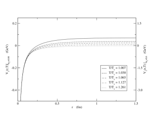
Figure 1:

Figure 2:

Figure 3:

Figure 4:

Figure 5:

Figure 6:

References

- [1] Yu.A.Simonov, JETP Lett. 54 (1991) 249.
- [2] Yu.A.Simonov, Phys. At. Nucl. 58 (1995) 309, hep-ph/9311216, JETP Lett. 55 (1992) 627.
-
[3]
Yu.A.Simonov, Lecture at the International School of Physics
”Enrico Fermi”, Varenna, 27 June–7 July 1995, ”Varenna 1995, selected topics
in nonperturbative QCD”, 319-337; hep-ph/9509404.;
Yu.A.Simonov, E.L.Gubankova, Phys. Lett. B360 (1995) 93;
N.O.Agasian, Phys. Lett. B562 (2003) 257. -
[4]
H.G.Dosch, Phys. Lett. B190 (1987) 177;
H.G.Dosch and Yu.A.Simonov, Phys. Lett. B205 (1988)339;
Yu.A.Simonov, Nucl. Phys. B307 (1988) 512. - [5] A.Di Giacomo, H.G.Dosch, V.I.Shevchenko and Yu.A.Simonov, Phys. Rept. 372 (2002) 319, hep-ph/0007223.
-
[6]
A.Di Giacomo and H.Panagopoulos, Phys. Lett. B285 (1992) 133;
M.D’Elia, A.Di Giacomo and E.Meggiolaro, Phys. Lett. B408 (1997) 315;
A.Di Giacomo, E.Meggiolaro and H.Panagopoulos, Nucl. Phys. B483 (1997) 371;
M.D’Elia, A.Di Giacomo and E.Meggiolaro, Phys. Rev. D67 (2003) 114504;
G.S.Bali, N.Brambilla, A.Vairo, Phys. Lett. B421 (1998) 265. - [7] E.Meggiolaro, Phys. Lett. B451 (1999) 414.
- [8] M.Asakawa, T.Hatsuda and Y.Nakahara, Nucl. Phys. A715 (2003) 701, hep-lat/0208059.
- [9] I.Wetzorke, F.Karsch, E.Laermann, P.Petreczky and S.Stickan, Nucl. Phys. Proc. Suppl. 106 (2002) 510, hep-lat/0110132.
- [10] T.Umeda, K.Nomura and H.Matsufuru, Eur. Phys. J. C39S1 (2005) 9, hep-lat/0211003.
- [11] M.Asakawa and T.Hatsuda, Phys. Rev. Lett. 92 (2004) 012001.
-
[12]
S.Datta, F.Karsch, P.Petreczky and I.Wetzorke, hep-lat/0208012;
Phys. Rev. D69 (2004) 094507;
F.Karsch et al. Nucl. Phys. A715 (2003) 863; P.Petreczky, J. Phys. G30 (2004) 431;
T.Umeda, H.Matsufuru, hep-lat/0501002. - [13] P.Petreczky, Plenary talk at Lattice 2004, hep-lat/0409139, P.Petreczky, hep-lat/0502008.
- [14] K.Hübner, O.Kaczmarek, F.Karsch, O.Vogt, hep-lat/0408031.
- [15] O.Kaczmarek, F.Karsch, P.Petreczky and F.Zantow, Phys. Lett. B543 (2002) 41, hep-lat/0207002.
- [16] O.Kaczmarek, F.Karsch, P.Petreczky and F.Zantow, Nucl. Phys. Proc. Suppl. 129, 560 (2004); hep-lat/0309121; hep-lat/0406036; M.Döring, S.Ejiri, O.Kaczmarek, F.Karsch, E.Laermann, hep-lat/0509150.
- [17] Yu.A.Simonov, Phys. Lett. B619 (2005) 293.
- [18] T.D.Lee, Nucl. Phys. A750 (2005) 1; M.Gyulassy, L.Mc Lerran, Nucl. Phys. A750 (2005) 30; E.V.Shuryak, Nucl. Phys. A750 (2005) 61.
- [19] Yu.A.Simonov, hep-ph/0501182.
-
[20]
Yu.A.Simonov, Yad.Fiz. 58 (1995) 113;
Yu.A.Simonov, in: ”Lecture Notes in Physics” H.Latal, W.Schweiger eds. Vol. 479, p. 138, Springer, 1996;
Yu.A.Simonov, Phys. Atom. Nucl. 65 (2002) 135, hep-ph/0109081;
Yu.A.Simonov, Phys. Atom. Nucl. 66 (2003) 764; hep-ph/0109159. - [21] Yu.A.Simonov, Phys. Atom. Nucl. 61, (1998) 855; hep-ph/9712250.
-
[22]
Yu.A.Simonov and J.A.Tjon, Ann. Phys. (NY) 228 (1993) 1;
Yu.A.Simonov and J.A.Tjon, Ann. Phys. 300 (2002) 54;
hep-ph/0205165. - [23] Yu.A.Simonov, Nucl. Phys. B592 (2001) 350, hep-ph/0003114.
- [24] M.A.Shifman, A.I.Vainshtein and V.I.Zakharov, Nucl. Phys.B147, 385 (1979).
- [25] Yu.A.Simonov, Nucl. Phys. B324 (1989) 67.
- [26] H.G.Dosch, M.Eidemüller and M.Jamin, Phys. Lett. B452, 379 (1999).
- [27] M. D’Elia, A. Di Giacomo and E. Meggiolaro, Phys. Rev. D 67 (2003) 114504.
-
[28]
A. Di Giacomo, E. Meggiolaro and H. Panagopoulos, Nucl. Phys. B
483 (1997) 371;
A. Di Giacomo, E. Meggiolaro and H. Panagopoulos, hep–lat/9603018. - [29] G. Boyd, J. Engels, F. Karsch, E. Laermann, C. Legeland, M. Lütgemeier and B. Petersson, Nucl. Phys. B 469 (1996) 419.
- [30] M. Eidemüller and M. Jamin, Phys. Lett. B 416 (1998) 415.
- [31] E.V.Shuryak and I.Zahed, Phys. Rev. D 70, 054507 (2004), hep-ph/0403127.
- [32] K.Hübner, O.Kaczmarek, F.Karsch, O.Vogt, hep-lat/0408031.
- [33] A.Yu.Dubin, A.B.Kaidalov, and Yu.A.Simonov, Phys. Lett. B 323, 4 (1994); Phys. At. Nucl. 56 (1993) 1745, hep-ph/9311344.
- [34] Yu.A.Simonov, in: ”QCD: Perturbative or nonperturbative?” Proceedings of the XVII Quantum School, Lisbon, 29 Sept. – 4 Oct., 1999, p. 60 (World Sci. 2000).
- [35] A.M.Badalian, B.L.G. Bakker, A.I.Veselov, Phys. Rev. D70, 016007 (2004).
- [36] Particle Data Group, Phys. Rev. D66, 89 (2002).
- [37] A.M.Badalian, A.I.Veselov, B.L.G.Bakker, Yad. Fiz. 67, 1392 (2004), hep-ph/0311010.
- [38] P.Petreczky et al., Nucl. Phys. Proc. Suppl. 106, 513 (2002).
- [39] P.Levai, U.W.Heinz, Phys. Rev. C57, 1879 (1998).
- [40] A.B.Kaidalov, Yu.A.Simonov, Phys. Lett. B 477, 163 (2000); Phys. At. Nucl. 63, 1428 (2000).
-
[41]
C.Morningstar, M.Peardon, Phys. Rev. D60,
034509 (1999);
M.J.Teper, Phys. Rev. D59, 014512 (1999). - [42] P.Petreczky, D.Patta, F.Karsch, I.Wetzorke, hep-lat/0309012.
- [43] N.Ishii, H.Suganuma, H,Matsufuru, Prog. Theor. Phys. Suppl. 151, 166 (2003); N.Ishii, H.Suganuma, hep-lat/0312040.
- [44] D.Blaschke, O.Kaczmarek, E.Laermann, V.Yudichev, Eur. Phys. J. C43, 81 (2005); hep-ph/0505053.
-
[45]
A.Mocsy, P.Petreczky, Eur. Phys. J. C43, 77
(2005);
W.M.Alberico, A.Beraudo, A.De Pace, A.Molinari, hep-ph/0507084. -
[46]
N.O.Agasian, JETP Lett. 57 (1993) 208;
N.O.Agasian, D.Ebert, E.-M.Ilgenfritz, Nucl. Phys. A637 (1998) 135;
A.Drago, M.Gibilisco, C.Ratti, Nucl. Phys. A742, 165 (2004). - [47] V. Vento, nucl-th/0509102.
- [48] E.V.Shuryak, A plenary talk at Quark Matter 05, Budapest, Aug. 2005, hep-ph/0510123.
- [49] Ch.-Y.Wong, Phys. Rev. C72, 034906 (2005).
- [50] Hong-Jo Park, C.-H.Lee, G.E.Brown, hep-ph/0503016.
- [51] P.Castorina, M.Mannarelli, hep-ph/0510349.
- [52] S.Ejiri, F.Karsch, K.Redlich, hep-ph/0509051.
- [53] V.Koch, A.Majumdar, J.Randrup, Nucl-th/0505052.