BYPASSING THE AXIAL ANOMALIES

Abstract

Many meson processes are related to the $U_{A}(1)$ axial anomaly, present in the Feynman graphs where fermion loops connect axial vertices with vector vertices. However, the coupling of pseudoscalar mesons to quarks does not have to be formulated via axial vertices. The pseudoscalar coupling is also possible, and this approach is especially natural on the level of the quark substructure of hadrons. In this paper we point out the advantages of calculating these processes using (instead of the anomalous graphs) the Feynman graphs where axial vertices are replaced by pseudoscalar vertices. We elaborate especially the case of the processes related to the Abelian axial anomaly of QED, but we speculate that it seems possible that effects of the non-Abelian axial anomaly of QCD can be accounted for in an analogous way.

PACS numbers: 14.40 -n, 12.39.Fe, 13.20.-v, 11.10.St

1 Introduction

Numerous processes in meson physics are related to the Adler-Bell-Jackiw (ABJ) axial anomaly [1, 2] appearing in the fermion loops connecting certain number of axial (A) and vector (V) vertices. Concretely, in this paper we will deal with the processes related to the AVV (“triangle”, Fig. 1) and VAAA (“box”, Fig. 2) anomaly, exemplified by the famous $\pi^{0}\to\gamma\gamma$ and $\gamma\to\pi^{+}\pi^{0}\pi^{-}$ transitions.

Figure 1: The triangle graph and its crossed graph relevant for the interaction of the neutral pseudoscalar meson of momentum $P$ with two photons of momenta $k$ and $k^{\prime}$. The quark-photon coupling is in general given by dressed vector vertices $\Gamma_{\mu}(q_{1},q_{2})$, which in the free limit reduce to $e{\cal Q}\gamma_{\mu}$.

Figure 2: One of the box diagrams for the process $\gamma\to\pi^{+}\pi^{0}\pi^{-}$, studied by the pseudoscalar coupling method in, e.g.,Refs. 3, 4. There are six different contributing graphs, obtained from the above graph by the permutations of the vertices of the three different pions. The position of the $u$ and $d$ quark flavors on the internal lines, as well as $Q_{u}$ or $Q_{d}$ quark charges in the quark-photon vertex, varies from graph to graph, depending on the position of the quark-pion vertices. The physical pion fields are $\pi^{\pm}=(\pi_{1}\mp i\pi_{2})/\sqrt{2}$ and $\pi^{0}\equiv\pi_{3}$. The momenta flowing through the four sections of the quark loop are conveniently given by various combinations of the symbols $\alpha,\beta,\gamma=+,0,-$ in $k_{\alpha\beta\gamma}\equiv k+\alpha p_{1}+\beta p_{2}+\gamma p_{3}$.

Suppose one wants to describe such processes using QCD-related effective chiral meson Lagrangians [5, 6] without adding ad hoc interactions of mesons with external gauge fields to reproduce empirical results. For example, one can add by hand

$$\Delta{\cal L}=g_{\pi\gamma\gamma}\pi^{0}\epsilon_{\mu\nu\rho\sigma}F^{\mu\nu}F^{\rho\sigma}\,,$$ (1)

and this would reproduce the observed $\pi^{0}\to\gamma\gamma$ width for the favorable value of the $\pi^{0}\gamma\gamma$ coupling $g_{\pi\gamma\gamma}$. However, if one does not want to add such ad hoc terms in the effective meson Lagrangians, one must describe such “anomalous” processes through the term derived by Wess and Zumino [7]. On the other hand, if one wants to utilize and explicitly take into account the fact that mesons are composed of quarks, another way of describing these processes is optimal in our opinion, and the main purpose of this paper is to stress and elucidate this.

Axial vertices in the anomalous graphs such as the AVV and VAAA ones, couple the quarks with pseudoscalar mesons. Instead of anomalous graphs, another way to study the related amplitudes involving pseudoscalar mesons, is to calculate the corresponding graphs where axial vertices (A) are replaced by pseudoscalar (P) ones. Thereby, for example, the $\pi^{0}\to\gamma\gamma$ decay amplitude due to the AVV “triangle anomaly”,

$$F_{m_{\pi}=0}(\pi^{0}\to 2\gamma)=\frac{e^{2}N_{c}}{12\pi^{2}f_{\pi}}~{},$$ (2)

is reproduced by the calculation of the PVV triangle graph. [Eq. (2) pertains to the chiral limit, where the pion mass $m_{\pi}=0$. Also, $f_{\pi}\approx 93~{}\mbox{\rm MeV}$ is the pion decay constant, $e$ is the proton charge, and $N_{c}=3$ is the number of quark colors.]

The PVV triangle graph calculation of Eq. (2) can most simply be done essentially à la Steinberger [8], that is, with a loop of “free” constituent quarks with the point pseudoscalar coupling (i.e., $g\gamma_{5}$, where $g=constant$) to quasi-elementary pion fields. However, since the development of the Dyson-Schwinger (DS) approach to quark-hadron physics [9, 10], the presently advocated method becomes even more convincing. Namely, the DS approach clearly shows how the light pseudoscalar mesons simultaneously appear both as quark-antiquark ($q\bar{q}$) bound states and as Goldstone bosons of the dynamical chiral symmetry breaking (D$\chi$SB) of nonperturbative QCD. The solutions of Bethe-Salpeter (BS) equations for the bound-state vertices of pseudoscalar mesons then enter in the PVV triangle graph instead of the point $g\gamma_{5}$ coupling, and the current algebra result (2) is again reproduced exactly and analytically, which is unique among the bound-state approaches. That the (almost massless) pseudoscalars are (quasi-)Goldstone bosons, is also a unique feature among the bound-state approaches to mesons.

A reason why the P-coupling method is simpler both technically and conceptually is that the PVV triangle graph amplitude is finite, unlike the AVV one, which is divergent and therefore also ambiguous with respect to the momentum routing. Reference Kekez:2005kx gives a more detailed discussion of the P-coupling method and why is that it is equivalent to the anomaly calculations, and illustrates this on the examples of the famous decay $\pi^{0}\to\gamma\gamma$ and processes of the type $\gamma\to\pi^{+}\pi^{0}\pi^{-}$. Also, the PVV quark triangle amplitude leads to many (over 15) decay amplitudes in agreement with data to within 3% and not involving free parameters [12, 13, 14]. This will be elaborated in more detail in Sec. 2. Additional advantages of this method is that its treatment of the $\eta$-$\eta^{\prime}$ complex and resolution of the $\rm U_{A}(1)$ problem, goes well with the absence of axions (which were predicted to solve the strong CP problem but have not yet been observed [15]) and with the arguments of Ref. Banerjee:2000qw, that there is really no strong CP problem. All this will be discussed in Sec. 3. We state our conclusions in Sec. 4.

2 Processes Going Through the Quark Triangle

In this section we calculate the amplitudes for a number of processes using the quark triangle graphs. Figures 1 and 3 show three such PVV processes. First we consider $\pi^{0}\to\gamma\gamma$ decay via the $u$ and $d$ quark triangle graph for $\pi^{0}=(\bar{u}u-\bar{d}d)/\sqrt{2}$, $N_{c}=3$ and Goldberger-Trieman relation leading to the pion decay constant: $f_{\pi}=\hat{m}/g_{\pi qq}$. This amplitude is finite and for the experimental value of the pion decay constant, $f_{\pi}=(92.42\pm 0.26)\,\mbox{\rm MeV}$ [15], gives [12] the chiral-limit amplitude (2) of magnitude

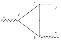
Figure 3: Two examples of the PVV triangle graphs where just one of the vector vertices couples to a photon, whereas the other couples to a vector meson. These two graphs describe the decays of $\omega$ and $\rho$ mesons into a photon and a pion.

$$|F_{m_{\pi}=0}(\pi^{0}\to 2\gamma)|=\frac{e^{2}}{4\pi^{2}f_{\pi}}=0.0251~{}\mbox{\rm GeV}^{-1}$$ (3)

very close to experimental data [15]

$$|F_{\rm exp}(\pi^{0}\to 2\gamma)|=\left[\frac{64\pi\Gamma(\pi^{0}\to\gamma\gamma)}{m_{\pi}^{3}}\right]^{1/2}=(0.0252\pm 0.0009)~{}\mbox{\rm GeV}^{-1}~{}.$$ (4)

Likewise, the $u$, $d$ quark triangles for $\rho\to\pi\gamma$ decay give [12]

$$|F(\rho\to\pi\gamma)|=\frac{eg_{\rho}}{8\pi^{2}f_{\pi}}=0.206~{}\mbox{\rm GeV}^{-1}$$ (5)

for $g_{\rho}=4.965\pm 0.002$ found from $\rho^{0}\to e^{-}e^{+}$ decay [15]:

$$\Gamma(\rho^{0}\to e^{-}e^{+})=\frac{e^{4}m_{\rho}}{12\pi g_{\rho}^{2}}=(7.02\pm 0.11)~{}\mbox{\rm keV}~{}.$$ (6)

The calculated $|F(\rho\to\pi\gamma)|$ is also near data [15],

$$|F_{\rm exp}(\rho\to\pi\gamma)|=\left[\frac{12\pi\Gamma(\rho\to\pi\gamma)}{q^{3}}\right]^{1/2}=(0.225\pm 0.011)~{}\mbox{\rm GeV}^{-1}~{},$$ (7)

where $q=(m_{\rho}^{2}-m_{\pi}^{2})/(2m_{\rho})$ is the photon momentum. [Actually, the above value is a weighted average of $F_{\rm exp}(\rho^{0}\to\pi^{0}\gamma)$ and $F_{\rm exp}(\rho^{\pm}\to\pi^{\pm}\gamma)$ amplitudes.]

Next we predict the $u$, $d$ quark triangle amplitude for $\omega\to\pi\gamma$ taking $\omega$ as 99% nonstrange [15] ($\cos^{2}\phi_{V}\approx 0.99$)

$$|F(\omega\to\pi\gamma)|=\frac{\cos\phi_{V}\,e\,g_{\omega}}{8\pi^{2}f_{\pi}}=0.705~{}\mbox{\rm GeV}^{-1}$$ (8)

for $g_{\omega}=17.06\pm 0.28$ found from $\omega\to e^{-}e^{+}$ decay. The mixing angle is

$$\phi_{V} = \theta_{V}-\arctan(\frac{1}{\sqrt{2}})=\arctan\sqrt{\frac{\frac{1}{3}(4m_{K^{\star}}^{2}-m_{\rho}^{2})-m_{\varphi}^{2}}{m_{\omega}^{2}-\frac{1}{3}(4m_{K^{\star}}^{2}-m_{\rho}^{2})}}-\arctan(\frac{1}{\sqrt{2}})$$ (9)

$$= (5.208\pm 0.092)^{\circ}~{}.$$

Again this theory in Eq. (8) is near data $(0.722\pm 0.012)~{}\mbox{\rm GeV}^{-1}$ [15].

Other PVV photon decays involve the $\eta$ and $\eta^{\prime}$ mixed non–strange and $\bar{s}s$ pseudoscalar mesons. Again the quark triangle amplitudes are a close match with data [12, 13, 14].

The quark–triangle (QT) calculation gives reliable predictions also for the $\eta$ and $\eta^{\prime}$ two–photon decays:

$$|F(\eta\to\gamma\gamma)|=\frac{e^{2}}{4\pi^{2}f_{\pi}}\frac{N_{c}}{9}(5\cos\phi_{P}-\sqrt{2}\frac{\hat{m}}{m_{s}}\sin\phi_{P})=0.0255\mbox{\rm GeV}^{-1}~{},$$ (10)

$$|F(\eta^{\prime}\to\gamma\gamma)|=\frac{e^{2}}{4\pi^{2}f_{\pi}}\frac{N_{c}}{9}(5\sin\phi_{P}+\sqrt{2}\frac{\hat{m}}{m_{s}}\cos\phi_{P})=0.0345~{}\mbox{\rm GeV}^{-1}~{}.$$ (11)

This should be compared with the experimental data:

$$|F_{\rm exp}(\eta\to\gamma\gamma)|=\left[\frac{64\pi\Gamma(\eta\to\gamma\gamma)}{m_{\eta}^{3}}\right]^{1/2}=(0.02498\pm 0.00064)~{}\mbox{\rm GeV}^{-1}~{},$$ (12)

$$|F_{\rm exp}(\eta^{\prime}\to\gamma\gamma)|=\left[\frac{64\pi\Gamma(\eta^{\prime}\to\gamma\gamma)}{m_{\eta^{\prime}}^{3}}\right]^{1/2}=(0.03133\pm 0.00055)~{}\mbox{\rm GeV}^{-1}~{},$$ (13)

where $\Gamma(\eta\to\gamma\gamma)=(0.5108\pm 0.0268)~{}\mbox{\rm keV}$ and $\Gamma(\eta^{\prime}\to\gamma\gamma)=(4.29\pm 0.15)~{}\mbox{\rm keV}$. The ratio of the constituent quark masses is $m_{s}/m=2f_{K}/f_{\pi}-1=1.445\pm 0.024$ for $f_{\pi^{\pm}}=(92.4\pm 0.3)~{}\mbox{\rm MeV}$ and $f_{K}=(113.0\pm 1.0)~{}\mbox{\rm MeV}$ [15]. The mixing angle is [18, 19]

$$\phi_{P} = \theta_{P}+\arctan({\sqrt{2}})=\arctan\sqrt{\frac{(m_{\eta^{\prime}}^{2}-2m_{K}^{2}+m_{\pi}^{2})(m_{\eta}^{2}-m_{\pi}^{2})}{(2m_{K}^{2}-m_{\pi}^{2}-m_{\eta}^{2})(m_{\eta^{\prime}}^{2}-m_{\pi}^{2})}}$$ (14)

$$= (42.441\pm 0.019)^{\circ}~{}.$$

Next, we can calculate the $\rho^{0}\to\eta\gamma$ amplitude employing the quark–triangle diagram,

$$|F(\rho^{0}\to\eta\gamma)|=\frac{eg_{\rho}}{8\pi^{2}f_{\pi}}3\cos\phi_{P}=0.456~{}\mbox{\rm GeV}^{-1}~{}.$$ (15)

Again, this is close to the experimental data,

$$|F_{\rm exp}(\rho^{0}\to\eta\gamma)|=\left[\frac{12\pi\Gamma(\rho^{0}\to\eta\gamma)}{q^{3}}\right]^{1/2}=(0.48\pm 0.03)~{}\mbox{\rm GeV}^{-1}~{},$$ (16)

where $q=(m_{\rho}^{2}-m_{\eta}^{2})/(2m_{\rho})=(194.5\pm 0.4)~{}\mbox{\rm MeV}$ is the photon momentum and $\Gamma(\rho^{0}\to\eta\gamma)=(45.1\pm 6.0)~{}\mbox{\rm keV}$. A similar situation is with the $\eta^{\prime}\to\rho\gamma$ amplitude, for which the quark–triangle calculation gives

$$|F(\eta^{\prime}\to\rho^{0}\gamma)|=\frac{eg_{\rho}}{8\pi^{2}f_{\pi}}3\sin\phi_{P}=0.417~{}\mbox{\rm GeV}^{-1}~{}.$$ (17)

The corresponding experimental value is

$$|F_{\rm exp}(\eta^{\prime}\to\rho^{0}\gamma)|=\left[\frac{4\pi\Gamma(\eta^{\prime}\to\rho^{0}\gamma)}{q^{3}}\right]^{1/2}=(0.411\pm 0.017)~{}\mbox{\rm GeV}^{-1}~{},$$ (18)

where $q=(m_{\eta^{\prime}}^{2}-m_{\rho}^{2})/(2m_{\eta^{\prime}})=(164.7\pm 0.4)~{}\mbox{\rm MeV}$ is the photon momentum and

$$\Gamma(\eta^{\prime}\to\rho^{0}\gamma\,\,\,\mbox{\rm including non--resonant}\,\,\,\pi^{+}\pi^{-}\gamma)=(60.0\pm 5.0)~{}\mbox{\rm keV}$$ (19)

is the experimental decay width [15].

The $\eta\to\pi\pi\gamma$ amplitude is

$$|M^{\mbox{\rm\scriptsize VMD}}_{\eta\to\pi\pi\gamma}|=|\frac{2g_{\rho\pi\pi}M^{\mbox{\rm\scriptsize QT}}_{\rho^{0}\to\eta\gamma}}{m_{\rho}^{2}-s}|=9.80~{}\mbox{\rm GeV}^{-3}$$ (20)

where $s=m_{\pi}^{2}$. The $\eta\to\pi\pi\gamma$ decay width is

$$\Gamma(\eta\to\pi\pi\gamma)=\frac{|M_{\eta\to\pi\pi\gamma}|^{2}}{(2\pi)^{3}}m_{\eta}^{7}Y_{\eta}=56.2~{}\mbox{\rm eV}~{},$$ (21)

where $Y_{\eta}=0.98\cdot 10^{-5}$ [20]. This is in a good agreement with the experimental value

$$\Gamma(\eta\to\pi\pi\gamma)=(60.4\pm 3.6)~{}\mbox{\rm eV}~{},$$ (22)

revealing that the vector meson dominance is the main effect, while the coupling through VPPP quark box loop (“contact term”) contributes little.

It is known that $\omega\to 3\pi$ decay is dominated by $\rho$–meson poles. The required $\omega\to\rho\pi$ amplitude can be estimated as

$$|M^{\mbox{\rm\scriptsize VMD}}(\omega\to\rho\pi)|=\left(\frac{g_{\rho}}{e}\right)|F(\omega\to\pi^{0}\gamma)|\sim 12~{}\mbox{\rm GeV}^{-1}~{},$$ (23)

but cannot be measured because there is no phase space for this process. The $\omega\to\rho\pi$ amplitude is more precisely defined with QL, additionally enhanced with a meson loop associated with sigma exchange [13, 14, 21],

$$|M(\omega\to\rho\pi)|_{\mbox{\rm\scriptsize QT}}=\frac{3g_{\rho\pi\pi}^{2}}{8\pi^{2}f_{\pi}}\approx 15~{}\mbox{\rm GeV}^{-1}~{}.$$ (24)

The scalar amplitude $M^{\mbox{\rm\scriptsize VMD}}(\omega\to 3\pi)$ is dominated by the $\rho$ meson in each of the three possible channels [22],

$$|M^{\mbox{\rm\scriptsize VMD}}(\omega\to 3\pi)| = 2g_{\rho\pi\pi}|M(\omega\to\rho\pi)|\left[\frac{1}{m_{\rho}^{2}-s}+\frac{1}{m_{\rho}^{2}-t}+\frac{1}{m_{\rho}^{2}-u}\right]$$ (25)

$$\approx 1480~{}\mbox{\rm GeV}^{-3}~{}.$$

Following Thew’s phase space analysis [20], we get

$$\Gamma(\omega\to\ 3\pi)=\frac{|M^{\mbox{\rm\scriptsize VMD}}(\omega\to 3\pi)|^{2}}{(2\pi)^{3}}m_{\omega}^{7}Y_{\omega}=7.3~{}\mbox{\rm MeV}$$ (26)

where $Y_{\omega}=4.57\cdot 10^{-6}$ is used. The predicted value is close to the experimental value [15]

$$\Gamma(\omega\to 3\pi)=(7.6\pm 0.1)~{}\mbox{\rm MeV}~{}.$$ (27)

Here we have taken $\omega$ as pure NS, although it is about 99% NS, since $\phi_{V}=(5.208\pm 0.092)^{\circ}$ from our Eq. (9).

In the quark–level $\sigma$–model a quark box diagram contributes to the $\omega\to 3\pi$ decay. This box diagram can be interpreted as a contact term. It is shown that the contact contribution is small by itself, but can be enlarged through the interference effect [23].

Using $\phi_{P}=(42.441\pm 0.019)^{\circ}$ from our Eq. (14), we predict the tensor $T\to PP$ branching ratios for $a_{2}(1320)$:

$$\begin{array}[]{ll}\mbox{\rm BR}(\frac{\textstyle{a_{2}\to\eta\pi}}{\textstyle{a_{2}\to K\bar{K}}})=\left(\frac{\textstyle{p_{\eta\pi}}}{\textstyle{p_{K}}}\right)^{5}2\cos^{2}\phi_{P}=2.996&(\mbox{\rm data}\,\,\,\,2.96\pm 0.54)~{},\\ \mbox{\rm BR}(\frac{\textstyle{a_{2}\to\eta^{\prime}\pi}}{\textstyle{a_{2}\to K\bar{K}}})=\left(\frac{\textstyle{p_{\eta^{\prime}\pi}}}{\textstyle{p_{K}}}\right)^{5}2\sin^{2}\phi_{P}=0.1113&(\mbox{\rm data}\,\,\,\,0.108\pm 0.025)~{},\\ \mbox{\rm BR}(\frac{\textstyle{a_{2}\to\eta^{\prime}\pi}}{\textstyle{a_{2}\to\eta\pi}})=\left(\frac{\textstyle{p_{\eta^{\prime}\pi}}}{\textstyle{p_{\eta\pi}}}\right)^{5}\tan^{2}\phi_{P}=0.0371&(\mbox{\rm data}\,\,\,\,0.0366\pm 0.0069)~{},\end{array}$$ (31)

for center of mass momenta $p_{\eta\pi}=535~{}\mbox{\rm MeV}$, $p_{\eta^{\prime}\pi}=287~{}\mbox{\rm MeV}$, $p_{K}=437~{}\mbox{\rm MeV}$. The above data branching ratios follow from $a_{2}(1320)$ recent fractions [15]: $\mbox{\rm BR}(a_{2}\to\eta\pi)=(14.5\pm 1.2)\%$, $\mbox{\rm BR}(a_{2}\to K\bar{K})=(4.9\pm 0.8)\%$ and $\mbox{\rm BR}(a_{2}\to\eta^{\prime}\pi)=(5.3\pm 0.9)\cdot 10^{-3}$.

3 Comments Related to the Gluon Anomaly

The approach using the pseudoscalar coupling is, in our opinion, also relevant for the effects related to the non-Abelian, “gluon” ABJ axial anomaly. Here, we comment on this only briefly, and direct the reader to the original references for details.

3.1 Goldstone structure and $\eta$-$\eta^{\prime}$ phenomenology

The first point concerns the $\eta$-$\eta^{\prime}$ complex and the $U_{A}(1)$ problem related to it.

In the chiral limit $m_{\pi}=m_{K}=m_{\eta_{8}}=0$, since all members of the flavor-SU(3) pseudoscalar meson octet are massless in this theoretical, but very useful limit. The only non-vanishing ground-state pseudoscalar meson mass in this limit is the mass of the SU(3)-singlet pseudoscalar meson $\eta_{1}$. This is thanks to the non-Abelian, gluon ABJ axial anomaly, i.e., to the fact that the divergence of the SU(3)-singlet axial current

$$A^{\mu}_{0}(x)=\overline{\Psi}(x)\gamma^{\mu}\gamma_{5}\Psi(x)\,,$$ (32)

receives the contributions from both the finite quark masses and gluon fields $G_{a}^{\mu\nu}$:

$$\partial_{\mu}A^{\mu}_{0}=2{\rm i}m_{u}\,\overline{u}\gamma_{5}u+2{\rm i}m_{d}\,\overline{d}\gamma_{5}d+2{\rm i}m_{s}\,\overline{s}\gamma_{5}s+\frac{3\,g^{2}}{32\pi^{2}}\epsilon_{\mu\nu\alpha\beta}G_{a}^{\mu\nu}G_{a}^{\alpha\beta}\,.$$ (33)

This removes the $U_{A}(1)$ symmetry and explains why only eight pseudoscalar mesons are light, and not nine; i.e., why there is an octet of (almost-)Goldstone bosons, but not a nonet. The physically observed $\eta$ and $\eta^{\prime}$ are then the mixtures of the anomalously heavy $\eta_{1}$ and (almost-)Goldstone $\eta_{8}$ in such a way that $\eta^{\prime}$ is predominantly $\eta_{1}$ and $\eta$ is predominantly $\eta_{8}$. This is how the gluon anomaly can save us from the $U_{A}(1)$ problem in principle, and the details of how we achieve a successful description of the $\eta$-$\eta^{\prime}$ complex, are given in Refs. Jones:1979ez,Kekez:2000aw,Klabucar:1997zi,Klabucar:2000me,Klabucar:2001gr. Here we just sketch some important points. The mass matrix squared $\hat{M}^{2}$ in the quark basis $|u\bar{u}\rangle$, $|d\bar{d}\rangle$, $|s\bar{s}\rangle$ is

$$\hat{M}^{2}=\hat{M}_{\mbox{\rm\scriptsize NA}}^{2}+\hat{M}_{\rm A}^{2}=\left[\begin{array}[]{ccc}m_{u\bar{u}}^{2}&0&0\\ 0&m_{d\bar{d}}^{2}&0\\ 0&0&m_{s\bar{s}}^{2}\end{array}\right]+\beta\left[\begin{array}[]{ccl}1&1&X\\ 1&1&X\\ X&X&X^{2}\end{array}\right]~{},$$ (34)

where $\hat{M}_{\mbox{\rm\scriptsize NA}}^{2}$ is the non-anomalous part of the matrix, since $m_{u\bar{u}}^{2}=m_{d\bar{d}}^{2}=m_{\pi}^{2}$ and $m_{s\bar{s}}^{2}=2m_{K}^{2}-m_{\pi}^{2}$ would be the masses of the respective “non-strange” (NS) and “strange” (S) pseudoscalar $q\bar{q}$ mesons if there were no gluon anomaly. In the NS sector, in the isospin symmetry limit (which is very close to reality), the relevant combinations are $|\pi^{0}\rangle=|u\bar{u}-d\bar{d}\rangle/\sqrt{2}$ as the neutral partner of the charged pions $|\pi^{\pm}\rangle$ in the isospin 1 triplet, and the isospin 0 combination $|u\bar{u}+d\bar{d}\rangle/\sqrt{2}$. In the absence of gluon anomaly, but with an $s$-quark mass heavier than the isosymmetric $u$ and $d$ ones, $\eta$ would reduce to $|{\rm NS}\rangle=|u\bar{u}+d\bar{d}\rangle/\sqrt{2}$ with the mass $m_{\mbox{\rm\scriptsize NS}}=m_{\pi}$, and $\eta^{\prime}$ to $|{\rm S}\rangle=|s\bar{s}\rangle$ with the mass $m_{\mbox{\rm\scriptsize S}}=m_{s\bar{s}}$. Both of these assignments are in conflict with experiment. The realistic contributions of various flavors to $\eta$ and $\eta^{\prime}$ and their masses (i.e., the realistic $\eta$-$\eta^{\prime}$ mixing) are obtained only thanks to $\hat{M}_{\rm A}^{2}$, the anomalous contribution to the mass matrix. In $\hat{M}_{\rm A}^{2}$, the quantity $\beta$ describes transitions $|q\bar{q}\rangle\to|q^{\prime}\bar{q}^{\prime}\rangle$ ($q,q^{\prime}=u,d,s$) due to the gluon anomaly and $X$ describes the effects of the SU(3) flavor symmetry breaking on these transitions. In Refs. Jones:1979ez,Kekez:2000aw,Klabucar:2000me, as the first step in solving the $U_{A}(1)$ problem, we extract $\eta_{8}$, $\eta_{1}$ masses from the $\eta$, $\eta^{\prime}$ via

$$m_{\eta_{8}}^{2}=(m_{\eta}\cos\theta_{P})^{2}+(m_{\eta^{\prime}}\sin\theta_{P})^{2}=(572.73~{}\mbox{\rm MeV})^{2}~{},$$ (35)

$$m_{\eta_{1}}^{2}=(m_{\eta}\sin\theta_{P})^{2}+(m_{\eta^{\prime}}\cos\theta_{P})^{2}=(943.05~{}\mbox{\rm MeV})^{2}~{},$$ (36)

where $\theta_{P}=\phi_{P}-\arctan(\sqrt{2})=(-12.295\pm 0.019)^{\circ}$. The mesons $\eta_{8}$ and $\eta_{1}$ are defined as

$$|\eta_{8}\rangle = \frac{1}{\sqrt{6}}(|u\bar{u}\rangle+|d\bar{d}\rangle-2|s\bar{s}\rangle)~{},$$ (37)

$$|\eta_{1}\rangle = \frac{1}{\sqrt{3}}(|u\bar{u}\rangle+|d\bar{d}\rangle+|s\bar{s}\rangle)~{}.$$ (38)

The $\eta_{8}$ meson mass (35) $m_{\eta_{8}}=572.73~{}\mbox{\rm MeV}$ is 4.56% greater than the observed [15] $m_{\eta}=(547.75\pm 0.12)~{}\mbox{\rm MeV}$. The singlet $\eta_{1}$ mass (36) $m_{\eta_{1}}=943.06~{}\mbox{\rm MeV}$ is only 1.56% below the observed $m_{\eta}^{\prime}=(957.78\pm 0.14)~{}\mbox{\rm MeV}$ and close to the nonstrange–$\bar{s}s$ mixing $U_{A}(1)$ mass dictated by phenomenology [18, 19, 25]

$$m_{U_{A}(1)}\equiv(3\beta)^{1/2}=\left[\frac{3}{4}\frac{(m_{\eta^{\prime}}^{2}-m_{\pi}^{2})(m_{\eta}^{2}-m_{\pi}^{2})}{m_{K}^{2}-m_{\pi}^{2}}\right]^{1/2}=915.31~{}\mbox{\rm MeV}~{},$$ (39)

(This is also close to $912~{}\mbox{\rm MeV}$, which is the mass found in the analogous DS approach [19, 25].)

We call the quantity (39) the “mixing $U_{A}(1)$ mass” since the mass matrix (which is especially clear in the nonstrange-strange quark basis) reveals that $m_{U_{A}(1)}$ induces the mixing between the nonstrange isoscalar $(|\bar{u}u\rangle+|\bar{d}d\rangle/\sqrt{2}$ and $\bar{s}s$ quark-antiquark states. Equivalently, $m_{U_{A}(1)}$ can be viewed as being generated by the transitions among the $\bar{u}u$, $\bar{d}d$ and $\bar{s}s$ pseudoscalar states; via quark loops, these pseudoscalar $\bar{q}q$ bound states can annihilate into gluons which in turn via another quark loop can again recombine into another pseudoscalar $\bar{q}^{\prime}q^{\prime}$ bound state of the same or different flavor. The quantity $\beta$ appearing in Eq. (39) is then the annihilation strength of such transitions, in the limit of an exact SU(3) flavor symmetry. (The realistic breaking of this symmetry is easily introduced and improves our description of the $\eta$-$\eta^{\prime}$ complex considerably.) The “diamond” graph in Fig. 4 gives just the simplest example of such an annihilation/recombination transition. Since these annihilations occur in the nonperturbative regime of QCD, all graphs with any even number of gluons instead of just those two in Fig. 4, can be just as significant in annihilating and forming a $C^{+}$ pseudoscalar $\bar{q}q$ meson. Indeed, this nonperturbative $U_{A}(1)$ mass scale, Eq. (39), is still 3 times higher than the gluon “diamond” graph evaluated perturbatively [27]. Thus, we cannot calculate $\beta=m_{U_{A}(1)}^{2}/3$ and the situation is much more complicated and less clear than in the Abelian case, as explained in [11]. Can it then be founded to think that the annihilation graphs with the pseudoscalar meson-quark coupling, such as the “diamond” graph in Fig. 4, give rise to the anomalous term $({3\,g^{2}}/{32\pi^{2}})\epsilon_{\mu\nu\alpha\beta}G_{a}^{\mu\nu}G_{a}^{\alpha\beta}$ in the divergence (33) of the SU(3)-singlet current $A^{\mu}_{0}(x)$, and thus ultimately to the large mass of $\eta_{0}$ (and of the observed $\eta^{\prime}$)? Well, this conjecture may remain a speculation since we cannot calculate $\beta$ due to the nonperturbative nature of the problem. Nevertheless, when we use it in our approach as a parameter with the value given by Eq. (39), we obtain a very good description of the $\eta$-$\eta^{\prime}$ complex phenomenology [18, 19, 24, 25, 26]. This includes not only the masses of $\eta$ and $\eta^{\prime}$, but also their $\gamma\gamma$ decay widths, and the mixing angle $\theta_{P}\approx-13^{\circ}$ consistently following from the masses and $\gamma\gamma$ widths. This gives a strong motivation for the above conjecture.

Figure 4: Nonperturbative QCD annihilation of a quark-antiquark bound state illustrated by the diagram with two-gluon exchange. The $\bar{q}q$ pseudoscalar $P$ is coupled to a quark loop, whereby it can annihilate into gluons which in turn recombine into the pseudoscalar $P^{\prime}$ having the flavor content $\bar{q^{\prime}}q^{\prime}$.

3.2 Taming of strong CP problem

We should also note that our conjecture in the previous subsection goes well with the arguments of Banerjee et al. [16], that there is really no strong CP problem. They find that one does not need vanishing $\Theta_{\rm eff}=\Theta-{\rm tr}\ln{\cal M}_{q}$ (where ${\cal M}_{q}$ is the quark mass matrix). Thus, one does not need any fine-tuning, and all CP violation in the QCD Lagrangian can be avoided by having $\Theta=0$ in its CP-violating term

$${\cal L}_{\Theta}=-\Theta\,\frac{g^{2}}{64\pi^{2}}\epsilon_{\mu\nu\alpha\beta}G_{a}^{\mu\nu}G_{a}^{\alpha\beta}\,.$$ (40)

This term in the QCD Lagrangian breaks the $U_{A}(1)$ symmetry and corresponds to the anomalous term $\propto\epsilon_{\mu\nu\alpha\beta}G_{a}^{\mu\nu}G_{a}^{\alpha\beta}$ in the divergence (33) of the singlet current. The term (40) is allowed by gauge invariance and renormalizability, but apparent nonexistence of the strong CP violation, and also of axions, is the solid reason to have it vanishing. Our conjecture, that P-coupled annihilation graphs reproduce the effect of the gluon ABJ anomaly, naturally agrees with the vanishing of this term and with putting the case of the strong CP problem to rest à la Banerjee et al. [16].

4 Summary/Discussion

We have presented and surveyed in detail the method of pseudoscalar coupling of pseudoscalar mesons to the “triangle” and “box” quark loops. We have reviewed how this method gives the equivalent results to the anomaly calculations. The P-coupling method has also been illustrated on the example of many decay amplitudes.

The AVV anomaly [1, 2] involves 10 invariant amplitudes (reduced to 1 or 2 amplitudes for $\pi^{0}\to\gamma\gamma$ decay using additional Ward identities). If instead one considers the PVV transition with a pseudoscalar coupling, then the PVV quark triangle amplitude is finite and leads to many decay amplitudes (over 15) then in agreement with data to within 3% and not involving free parameters [12]. To solve instead the former AVV decay problem, very light axion bosons have been predicted but have not yet been observed [15].

Also, there is the $U_{A}(1)$ and $\Theta$ problem involving gluons whereby strong interaction QCD leads to CP violation, definitely a “strong CP problem” because CP violation is known to occur at the $10^{-3}$ weak interaction amplitude level [15]. Physicists have tried to circumvent this “$U_{A}(1)$ – strong CP problem” either via the topology of gauge fields or by investigating the $\Theta$–vacuum for this strong CP problem [16].

In this paper we have circumvented the need to deal directly with the above photon or gluon AVV anomalies by studying instead (finite) PVV quark triangle graphs. Then we have given our phenomenological results – which always are in approximate agreement with the data. Next we return to the $U_{A}(1)$ problem and again use quark triangle diagrams coupled to 2 gluons. Invoking nonstrange–strange particle mixing, the predicted $U_{A}(1)$ mass is within 3% of data [18, 19, 25].

Thus we circumvent both photon and, admittedly on a much more speculative level, also the gluon ABJ anomaly without resorting either to unmeasured axions or to a strong CP violating term in the QCD Lagrangian.

References

- [1] S. L. Adler, Phys. Rev. 177, 2426 (1969).
- [2] J. S. Bell and R. Jackiw, Nouvo Cim. A 60, 47 (1969).
- [3] B. Bistrović and D. Klabučar, Phys. Rev. D 61, 033006 (2000) [arXiv:hep-ph/9907515].
- [4] B. Bistrović and D. Klabučar, Phys. Lett. B 478, 127 (2000) [arXiv:hep-ph/9912452].
- [5] See, for example, Ref. \refciteGeorgi:1985kw by H. Georgi, and Chap. 5 of its updated version available in electronic form at http://schwinger.harvard.edu/~georgi/weak5.ps.
- [6] H. Georgi, “Weak Interactions And Modern Particle Theory”, Benjamin/Cummings, Menlo Park, USA (1984).
- [7] J. Wess and B. Zumino, Phys. Lett. B 37, 95 (1971).
- [8] J. Steinberger, Phys. Rev. 76, 1180 (1949).
- [9] R. Alkofer and L. von Smekal, Phys. Rept. 353, 281 (2001) [arXiv:hep-ph/0007355].
- [10] P. Maris and C.D. Roberts, Int. J. Mod. Phys. E 12, 297 (2003) [arXiv:nucl-th/0301049].
- [11] D. Kekez, D. Klabucar and M. D. Scadron, Fizika B 14, 13 (2005) [arXiv:hep-ph/0503141].
- [12] R. Delbourgo, Dongsheng Liu and M. D. Scadron, Int. J. Mod. Phys. A 14, 4331 (1999) [arXiv:hep-ph/9905501]; M. D. Scadron, F. Kleefeld, G. Rupp and E. van Beveren, Nucl. Phys. A 724, 391 (2003) [hep-ph/0211275].
- [13] R. Delbourgo and M. D. Scadron, Mod. Phys. Lett. A 10, 251 (1995) [arXiv:hep-ph/9910242].
- [14] A. Bramon, Riazuddin and M. D. Scadron, J. Phys. G 24, 1 (1998) [arXiv:hep-ph/9709274].
- [15] S. Eidelman et al., Phys. Lett. B 592, 1 (2004).
- [16] H. Banerjee, D. Chatterjee and P. Mitra, Phys. Lett. B 573, 109 (2003) [arXiv:hep-ph/0012284].
- [17] K. Hagiwara et al., Phys. Rev. D 66, 010001 (2002).
- [18] H. F. Jones and M. D. Scadron, Nucl. Phys. B 155, 409 (1979).
- [19] D. Kekez, D. Klabučar and M. D. Scadron, J. Phys. G 26, 1335 (2000) [arXiv:hep-ph/0003234].
- [20] R. L. Thews, Phys. Rev. D 10, 2993 (1974).
- [21] P. G. O. Freund and S. Nandi, Phys. Rev. Lett. 32, 181 (1974); S. Rudaz, Phys. Lett. B 145, 281 (1984).
- [22] M. Gell-Mann, D. Sharp and W. Wagner, Phys. Rev. Lett. 8, 261 (1962).
- [23] J. L. Lucio-Martinez, M. Napsuciale, M. D. Scadron and V. M. Villanueva, Phys. Rev. D 61, 034013 (2000).
- [24] D. Klabučar and D. Kekez, Phys. Rev. D 58, 096003 (1998) [arXiv:hep-ph/9710206].
- [25] D. Klabučar, D. Kekez and M. D. Scadron, arXiv:hep-ph/0012267.
- [26] D. Kekez, D. Klabučar and M. D. Scadron, J. Phys. G 27, 1775 (2001) [arXiv:hep-ph/0101324].
- [27] S. R. Choudhury and M. D. Scadron, Mod. Phys. Lett. A 1, 535 (1986).