Abstract

We discuss and compare different approaches to include gluon transverse momenta for heavy quark-antiquark pair production. The correlations in azimuthal angle and in heavy quark, heavy antiquark transverse momenta are studied in detail. The results are illustrated with the help of different unintegrated gluon distribution functons (UGDF) from the literature. We compare results obtained with on-shell and off-shell matrix elements and kinematics and quantify where these effects are negligible and where they are essential. We concentrate on the region of asymmetric transverse momenta of charm quark and charm antiquark. Most of UGDFs lead in this corner of the phase space to almost full decorellation in azimuthal angle. We propose correlation observables to be best suited in order to test the existing models of UGDFs.

PACS: 12.38.-t, 12.38.Cy, 14.65.Dw

1 Introduction

The charm-anticharm production in photo- and hadroproduction is known as one of the crucial tests of conventional gluon distributions within a standard factorization approach. At high energies one tests gluon distributions at low values of longitudinal momentum fraction. At leading order of collinear approach the heavy quark and heavy antiquark are produced back to back i.e. the azimuthal correlation function is proportional to $\delta(\phi-\pi)$ and the distribution in $p_{1,t}$ (heavy quark transverse momentum) and $p_{2,t}$ (heavy antiquark transverse momentum) is proportional to $\delta(p_{1,t}-p_{2,t})$. In collinear approach this changes only in next-to-leading order. In unintegrated gluon distribution approach the azimuthal angle and $p_{t}$ decorrelations are obtained already in leading order of perturbative expansion.

Different models of UGDF were presented in the literature. Recently we have tested some of the models in photoproduction [1]. Here we shall discuss in detail the case of hadroproduction.

It was realized recently that the understanding of transverse momenta can be a clue to understand many high energy reactions. In some reactions like meson hadroproduction, prompt photon and Drell-Yan production or single spin asymmetry (SSA) the transverse momenta are not obtained dynamically but are included “by hand” with Gaussian smearing (see e.g. [2, 3]). The parameter of the smearing is assumed to be independent of longitudinal momentum fraction and is usually arbitrarily chosen or adjusted to a selected set of data.

In some of high-energy reactions that involve gluons the unintegrated gluon distributions are modelled or are obtained as a solution of some (usually simplified) QCD evolution equations. In particular, the charm-anticharm hadroproduction is considered as one of the flag processes for the so-called $k_{t}$-factorization approach [4, 5, 6]. There are already a few phenomenological trials to calculate the charm or bottom production within the $k_{t}$-factorization approach [7, 8, 9]. The results of these trials differ considerably due to completely different UGDFs used.

In the present paper we shall compare different approaches how to include transverse momenta proposed in the literature for the charm-anticharm pair production at the Tevatron energy W = 1.96 GeV both for the single charm/anticharm distributions as well as for a few charm-anticharm correlation observables.

2 Formalism

Let us consider the reaction $h_{1}+h_{2}\to Q+\bar{Q}+X$, where $Q$ and $\bar{Q}$ are heavy quark and heavy antiquark, respectively. In the leading-order (LO) approximation within collinear approach the triple-differential cross section in rapidity of $Q$ ($y_{1}$), in rapidity of $\bar{Q}$ ($y_{2}$) and transverse momentum of one of them ($p_{t}$) can be written as

$$\frac{d\sigma}{dy_{1}dy_{2}d^{2}p_{t}}=\frac{1}{16\pi^{2}{\hat{s}}^{2}}\sum_{i,j}x_{1}p_{i}(x_{1},\mu^{2})\;x_{2}p_{j}(x_{2},\mu^{2})\;\overline{|{\cal M}_{ij}|^{2}}\;.$$ (1)

Above $p_{i}(x_{1},\mu^{2})$ and $p_{j}(x_{2},\mu^{2})$ are familiar (integrated) parton distributions in hadron $h_{1}$ and $h_{2}$, respectively. There are two types of LO $2\to 2$ subprocesses which enter Eq.(1): $gg\to Q\bar{Q}$ and $q\bar{q}\to Q\bar{Q}$. The first mechanism dominates at large energies and the second near the threshold. The parton distributions are evaluated at: $x_{1}=\frac{m_{t}}{\sqrt{s}}\left(\exp(y_{1})+\exp(y_{2})\right)$, $x_{2}=\frac{m_{t}}{\sqrt{s}}\left(\exp(-y_{1})+\exp(-y_{2})\right)$, where $m_{t}=\sqrt{p_{t}^{2}+m_{Q}^{2}}$. The formulae for matrix element squared averaged over initial and summed over final spin polarizations can be found e.g. in Ref.[10].

If one allows for transverse momenta of the initial partons, the sum of transverse momenta of the final $Q$ and $\bar{Q}$ no longer cancels. Formula (1) can be easily generalized if one allows for the initial parton transverse momenta. Then

$$\frac{d\sigma}{dy_{1}dy_{2}d^{2}p_{1,t}d^{2}p_{2,t}}=\sum_{i,j}\;\int\frac{d^{2}\kappa_{1,t}}{\pi}\frac{d^{2}\kappa_{2,t}}{\pi}\frac{1}{16\pi^{2}(x_{1}x_{2}s)^{2}}\;\overline{|{\cal M}_{ij}|^{2}}$$

$$\delta^{2}\left(\vec{\kappa}_{1,t}+\vec{\kappa}_{2,t}-\vec{p}_{1,t}-\vec{p}_{2,t}\right)\;{\cal F}_{i}(x_{1},\kappa_{1,t}^{2})\;{\cal F}_{j}(x_{2},\kappa_{2,t}^{2})\;,$$ (2)

where now ${\cal F}_{i}(x_{1},\kappa_{1,t}^{2})$ and ${\cal F}_{j}(x_{2},\kappa_{2,t}^{2})$ are so-called unintegrated parton distributions . The extra integration is over transverse momenta of the initial partons. The two extra factors $1/\pi$ attached to the integration over $d^{2}\kappa_{1,t}$ and $d^{2}\kappa_{2,t}$ instead over $d\kappa_{1,t}^{2}$ and $d\kappa_{2,t}^{2}$ as in the conventional relation between unintegrated ($\cal F$) and integrated ($g$) parton distributions. The two-dimensional Dirac delta function assures momentum conservation. Now the unintegrated parton distributions must be evaluated at: $x_{1}=\frac{m_{1,t}}{\sqrt{s}}\left(\exp(y_{1})+\exp(y_{2})\right)$, $x_{2}=\frac{m_{2,t}}{\sqrt{s}}\left(\exp(-y_{1})+\exp(-y_{2})\right)$, where $m_{i,t}=\sqrt{p_{i,t}^{2}+m_{Q}^{2}}$. In general, the matrix element must be calculated for initial off-shell partons. The corresponding formulae for initial gluons were calculated in [4, 5] (see also [6]). In the present paper for illustration we shall compare results obtained for both on-shell and off-shell matrix elements. It is easy to check that in the limit $\kappa_{1}^{2}\to 0$, $\kappa_{2}^{2}\to 0$

$$\begin{split}&|{\cal M}_{gg\to Q\bar{Q}}^{off-shell}|^{2}\to|{\cal M}_{gg\to Q\bar{Q}}^{on-shell}|^{2}=2\pi^{2}\alpha_{s}^{2}(...)\\ &\left[\frac{6(m_{Q}^{2}-\hat{t})(m_{Q}^{2}-\hat{u})}{\hat{s}^{2}}-\frac{m_{Q}^{2}(\hat{s}-4m_{Q}^{2})}{3(m_{Q}^{2}-\hat{t})(m_{Q}^{2}-\hat{u})}\right.\\ &+\frac{4}{3}\cdot\frac{(m_{Q}^{2}-\hat{t})(m_{Q}^{2}-\hat{u})-2m_{Q}^{2}(m_{Q}^{2}+\hat{t})}{(m_{Q}^{2}-\hat{t})^{2}}+\frac{4}{3}\cdot\frac{(m_{Q}^{2}-\hat{u})(m_{Q}^{2}-\hat{t})-2m_{Q}^{2}(m_{Q}^{2}+\hat{u})}{(m_{Q}^{2}-\hat{u})^{2}}\\ &\left.-3\cdot\frac{(m_{Q}^{2}-\hat{t})(m_{Q}^{2}-\hat{u})+m_{Q}^{2}(\hat{u}-\hat{t})}{\hat{s}(m_{Q}^{2}-\hat{t})}-3\cdot\frac{(m_{Q}^{2}-\hat{u})(m_{Q}^{2}-\hat{t})+m_{Q}^{2}(\hat{t}-\hat{u})}{\hat{s}(m_{Q}^{2}-\hat{u})}\right]\;,\end{split}$$ (3)

where $\hat{t},\hat{u},\hat{s}$ are Mendelstam variables for the partonic subprocess.

Introducing new variables:

$$\vec{Q}_{t}=\vec{\kappa}_{1,t}+\vec{\kappa}_{2,t}\;,$$

$$\vec{q}_{t}=\vec{\kappa}_{1,t}-\vec{\kappa}_{2,t}\;$$ (4)

we can write:

$$\frac{d\sigma_{ij}}{dy_{1}dy_{2}d^{2}p_{1,t}d^{2}p_{2,t}}=\int d^{2}q_{t}\;\frac{1}{4\pi^{2}}\frac{1}{16\pi^{2}(x_{1}x_{2}s)^{2}}\;\overline{|{\cal M}_{ij}|^{2}}$$

$${\cal F}_{i}(x_{1},\kappa_{1,t}^{2})\;{\cal F}_{j}(x_{2},\kappa_{2,t}^{2})\;.$$ (5)

This formula is very useful to study correlations between the produced heavy quark $Q$ and heavy antiquark $\bar{Q}$.

For example

$$\frac{d\sigma_{ij}}{dp_{1,t}dp_{2,t}} = \int d\phi_{1}d\phi_{2}\;p_{1,t}p_{2,t}\int dy_{1}dy_{2}\int d^{2}q_{t}\;\frac{1}{4\pi^{2}}\frac{1}{16\pi^{2}(x_{1}x_{2}s)^{2}}\;\overline{|{\cal M}_{ij}|^{2}}$$ (6)

$${\cal F}_{i}(x_{1},\kappa_{1,t}^{2})\;{\cal F}_{j}(x_{2},\kappa_{2,t}^{2})$$

$$= 4\pi\;\frac{1}{2}\;\frac{1}{2}\;\int d\phi_{-}\;p_{1,t}p_{2,t}\int dy_{1}dy_{2}\int d^{2}q_{t}\;\frac{1}{4\pi^{2}}\frac{1}{16\pi^{2}(x_{1}x_{2}s)^{2}}\;\overline{|{\cal M}_{ij}|^{2}}$$

$${\cal F}_{i}(x_{1},\kappa_{1,t}^{2})\;{\cal F}_{j}(x_{2},\kappa_{2,t}^{2})\;.$$

In the last equation we have introduced $\phi_{-}\equiv\phi_{1}-\phi_{2}$, where $\phi_{-}\in$ (-2$\pi$, 2$\pi$). The factor 4 $\pi$ comes from the integration over $\phi_{+}\equiv\phi_{1}+\phi_{2}$. The first factor 1/2 comes from the jacobian transformation while the second factor 1/2 takes into account an extra extension of the domain when using $\phi_{+}$ and $\phi_{-}$ instead of $\phi_{1}$ and $\phi_{2}$.

At the Tevatron energy the contribution of the $gg\to Q\bar{Q}$ subrocess is more than order of magnitude larger than its counterpart for the $q\bar{q}\to Q\bar{Q}$ subprocess. Therefore in the following we shall take into account only gluon-gluon fusion process i.e. i=0 and j=0. The quark-antiquark mechanism is important only at small center-of-mass energies.

In LO collinear approach

$$\frac{d\sigma}{dp_{1,t}dp_{2,t}}\propto\delta(p_{1,t}-p_{2,t})\;.$$ (7)

A deviation from this relation is therefore a measure of the initial gluon (parton) transverse momenta.

Purely perturbative $k_{t}$-factorization formalism to $h_{1}h_{2}\to Q\bar{Q}$ applies if $\kappa_{1,t}^{2},\kappa_{2,t}^{2}>\kappa_{0}^{2}$. The choice of $\kappa_{0}^{2}$ is to large extent arbitrary. In Refs.[7] a rather large $\kappa_{0}^{2}$ was chosen and the space $\kappa_{1,t}^{2}\times\kappa_{2,t}^{2}$ was subdivided into four disjoint regions. For example the contribution when both $\kappa_{1,t}^{2}$ and $\kappa_{2,t}^{2}$ are small was replaced by the leading-order collinear cross section. Such an approach by construction assures that $\sigma_{Q\bar{Q}}^{tot}>\sigma_{Q\bar{Q}}^{tot}$(collinear LO).
It is rather obvious that the total cross section strongly depends on the choice of $\kappa_{0}^{2}$. Our philosophy here is different. Many models of UGDF in the literature treat the soft region explicitly. Therefore we use the $k_{t}$-factorization formula everywhere on the $\kappa_{1,t}^{2}\times\kappa_{2,t}^{2}$ plane. For perturbatively generated UGDFs, like KMR [17] for instance, we shall extrapolate the perturbative behaviour into the soft region. Thus our approach guarantees a smooth behaviour on the $\kappa_{1,t}^{2}\times\kappa_{2,t}^{2}$ plane and reduces arbitrariness in dividing the two-dimensional gluon-transverse-momentum space.

3 Unintegrated gluon distributions

Obtaining UGDFs from underlying QCD is not an easy task. The main reason is the difficulty in separating out the perturbative from nonperturbative domains. The nonperturbative domain is difficult per se. Even in perturbative region different schemes of resummation have been proposed. In this section we describe briefly some representative UGDFs from the literature used in the present paper to calculate charm-anticharm production.

3.1 Kwieciński gluon distribution

Kwieciński has shown that the evolution equations for unintegrated parton distributions takes a particularly simple form in the variable conjugated to the parton transverse momentum. The two possible representations are interrelated via Fourier-Bessel transform

$$\begin{split}&{{\cal F}_{k}(x,\kappa_{t}^{2},\mu_{F}^{2})=\int_{0}^{\infty}db\;bJ_{0}(\kappa_{t}b){\tilde{\cal F}}_{k}(x,b,\mu_{F}^{2})}\;,\\ &{{\tilde{\cal F}}_{k}(x,b,\mu_{F}^{2})=\int_{0}^{\infty}d\kappa_{t}\;\kappa_{t}J_{0}(\kappa_{t}b){\cal F}_{k}(x,\kappa_{t}^{2},\mu_{F}^{2})}\;.\end{split}$$ (8)

The index k above numerates either gluons (k=0), quarks (k$>$ 0) or antiquarks (k$<$ 0).

In the impact-parameter space the Kwieciński equation takes a rather simple (diagonal in b) form [11, 12, 13] (see also [15]).

The perturbative solutions ${\tilde{\cal F}}_{q}^{pert}(x,b,\mu_{F}^{2})$ do not include nonperturbative effects such as, for instance, intrinsic transverse momenta of partons in colliding hadrons. One of the reasons is e.g. internal motion of constituents of the proton. In order to include such effects we modify the perturbative solution $\tilde{{\cal F}}_{g}^{pert}(x,b,\mu_{F}^{2})$ and write the modified parton distributions $\tilde{\cal{F}}_{g}(x,b,\mu_{F}^{2})$ in the simple factorized form

$$\tilde{{\cal F}}_{g}(x,b,\mu_{F}^{2})=\tilde{{\cal F}}_{g}^{pert}(x,b,\mu_{F}^{2})\cdot F_{g}^{np}(b)\;.$$ (9)

In the present study we shall use the following functional form for the nonperturbative form factor

$$F_{g}^{np}(b)=F^{np}(b)=\exp\left(-\frac{b^{2}}{4b_{0}^{2}}\right)\;.$$ (10)

In Eq.(10) $b_{0}$ is the only free parameter.

In the following we use leading-order integrated parton distributions from Ref.[25] as the initial condition for QCD evolution. The set of integro-differential equations in b-space is solved by the method based on the discretisation made with the help of the Chebyshev polynomials (see e.g. [13]). Then the unintegrated parton distributions $\tilde{{\cal F}}_{g}(x,b,\mu_{F}^{2})$ are put on a grid in $x$, $b$ and $\mu^{2}$ and the grid was used in practical applications for Chebyshev interpolation. In our practical application we need rather gluon distributions in momentum space. The latter are obtained via Fourier transform (8) from $\tilde{{\cal F}}_{g}(x,b,\mu_{F}^{2})$.

3.2 Kimber-Martin-Ryskin distribution

Resumming virtual contributions to DGLAP equation, the unintegrated parton distributions can be written as [17]

$$f_{a}(x,\kappa^{2},\mu_{F}^{2})=T_{a}(\kappa^{2},\mu_{F}^{2})\cdot\frac{\alpha_{s}(\kappa^{2})}{2\pi}\sum_{a^{\prime}}\int_{x}^{1-\delta}P_{aa^{\prime}}(z)\left(\frac{x}{z}\right)a^{\prime}\left(\frac{x}{z},\kappa^{2}\right)dz\;.$$ (11)

Specializing to the gluon distribution the Sudakov form factor reads as

$$T_{g}(\kappa^{2},\mu_{F}^{2})=\exp\left(-\int_{\kappa^{2}}^{\mu_{F}^{2}}\frac{dp^{2}}{p^{2}}\frac{\alpha_{s}(p^{2})}{2\pi}\int_{0}^{1-\delta}dz\left[zP_{gg}(z)+\sum_{q}P_{qg}(z)\right]\right)\;.$$ (12)

The Sudakov form factor introduces a dependence on a second scale $\mu_{F}^{2}$. Different prescriptions for $\delta$ have been used in the literature. The most popular choice $\delta=\mu_{F}/(\mu_{F}+\kappa)$ corresponds to the angular ordering in the gluon emission.

It is reasonable to assume that the unintegrated gluon density given by (11) starts only at $\kappa_{t}^{2}>\kappa_{t0}^{2}$ [18], i.e. in the perturbative domain. At lower $\kappa_{t}^{2}$ an extrapolation is needed. A use of the GRV integrated gluon distribution [24, 25] in (11) seems more adequate than any other gluon distribution because it allows to go down to small gluon transverse momenta. Following Ref.[16] $\kappa_{t0}^{2}$ = 0.5 GeV² is taken as the lowest value where the unintegrated gluon distribution is calculated from Eq.(11). Below it is assumed

$${\cal F}(x,\kappa^{2})=f(x,\kappa^{2})/\kappa^{2}=f(x,\kappa_{0}^{2})/\kappa_{0}^{2}\;.$$ (13)

In general, the quantity $\kappa_{t0}^{2}$ can be treated as a free nonperturbative parameter.

The choice of $\mu_{F}^{2}$ in our case of charmed quark-antiquark production is not completely obvious. In the present analysis, because we limit to not too large quark/antiquark transverse momenta, $\mu_{F}^{2}=m_{c}^{2},4m_{c}^{2}$ is taken for simplicity. This allows to prepare a two-dimensional grid ${\cal F}_{KMR}(x_{i},\kappa_{j}^{2})$ to be used for further interpolation in the $k_{t}$-factorization formula which accelerates the multi-dimensional integrations.

If $T_{g}$ in Eq.(11) is ignored we shall denote the corresponding gluon distribution as $f_{DGLAP}$ or ${\cal F}_{DGLAP}$ and call it DGLAP gluon distribution for brevity.

3.3 BFKL gluon distribution

At very low $x$ the unintegrated gluon distributions are believed to fulfil BFKL equation [19]. After some simplifications [20] the BFKL equation reads

$$-x\frac{\partial f(x,q_{t}^{2})}{\partial x}=\frac{\alpha_{s}N_{c}}{\pi}q_{t}^{2}\int_{0}^{\infty}\frac{dq_{1t}^{2}}{q_{1t}^{2}}\left[\frac{f(x,q_{1t}^{2})-f(x,q_{t}^{2})}{|q_{t}^{2}-q_{1t}^{2}|}+\frac{f(x,q_{t}^{2})}{\sqrt{q_{t}^{4}+4q_{1t}^{4}}}\right]\;.$$ (14)

The homogeneous BFKL equation can be solved numerically [20]. Here in the practical applications we shall use a simple parametrization for the solution [21]

$$f(x,\kappa_{t}^{2})=\frac{C}{x^{\lambda}}\left(\frac{\kappa_{t}^{2}}{q_{0}^{2}}\right)^{1/2}\frac{{\tilde{\phi}}_{0}}{\sqrt{2\pi\lambda^{\prime\prime}\ln(1/x)}}\exp\left[-\frac{\ln^{2}(\kappa_{t}^{2}/{\bar{q}}^{2})}{r2\lambda^{\prime\prime}\ln(1/x)}\right]\;.$$ (15)

In the above expression $\lambda=4{\bar{\alpha}}_{s}\ln 2$, $\lambda^{\prime\prime}$ = 28 ${\bar{\alpha}}_{s}\zeta(3)$, ${\bar{\alpha}}_{s}=3\alpha_{s}/\pi,\zeta(3)$ = 1.202. The remaining parameters were adjusted in [21] to reproduce with a satisfactory accuracy the gluon distribution which was obtained in [20] as the numerical solution of the BFKL equation. It was found that ${\bar{q}}=q_{0}$ = 1, $C{\bar{\phi}_{0}}$ = 1.19 and $r$ = 0.15 [21].

3.4 Golec-Biernat–Wüsthoff gluon distribution

Another parametrization of gluon distribution in the proton can be obtained based on the Golec-Biernat–Wüsthoff parametrization of the dipole-nucleon cross section with parameters fitted to the HERA data. The dipole-nucleon cross section can be transformed to corresponding unintegrated gluon distribution. The resulting gluon distribution reads [22]:

$$\alpha_{s}{\cal F}(x,\kappa_{t}^{2})=\frac{3\sigma_{0}}{4\pi^{2}}R_{0}^{2}(x)\kappa_{t}^{2}\exp(-R_{0}^{2}(x)\kappa_{t}^{2})\;,$$ (16)

where

$$R_{0}(x)=\left(\frac{x}{x_{0}}\right)^{\lambda/2}\frac{1}{GeV}\;.$$ (17)

From their fit to the data: $\sigma_{0}$ = 29.12 mb, $x_{0}$ = 0.41 $\cdot$ 10^-4, $\lambda$ = 0.277. In order to determine the gluon distribution we take somewhat arbitrarily $\alpha_{s}$ = 0.2.

3.5 Gluon distribution a la Kharzeev-Levin

Another parametrization, also based on the idea of gluon saturation, was proposed in [23]. In contrast to the GBW approach [22], where the dipole-nucleon cross section is parametrized, in the Karzeev-Levin approach it is the unintegrated gluon distribution which is parametrized. In the following we shall consider the most simplified functional form:

$${\cal F}(x,\kappa^{2})=\begin{cases}f_{0}&\text{if}\;\kappa^{2}<Q_{s}^{2},\\ f_{0}\cdot\frac{Q_{s}^{2}}{\kappa^{2}}&\text{if}\;\kappa^{2}>Q_{s}^{2}.\end{cases}$$ (18)

The saturation momentum $Q_{s}$ is parametrized exactly as in the GBW model $Q_{s}^{2}(x)=$ 1 GeV² $\cdot\left(\frac{x_{0}}{x}\right)^{\lambda}$.

The normalization constant $f_{0}$ was adjusted in [16] to roughly describe the HERA data.

3.6 Naive Gaussian smearing

For better understanding we shall compare our results with the results obtained with a simple unintegrated gluon distribution:

$${\cal F}_{naive}(x,\kappa^{2},\mu_{F}^{2})=xg^{coll}(x,\mu_{F}^{2})\cdot f_{Gauss}(\kappa^{2})\;,$$ (19)

where $g^{coll}(x,\mu_{F}^{2})$ is a standard collinear (integrated) gluon distribution and $f_{Gauss}(\kappa^{2})$ is a Gaussian two-dimensional function:

$$f_{Gauss}(\kappa^{2})=\frac{1}{2\pi\sigma_{0}^{2}}\exp\left(-\kappa_{t}^{2}/2\sigma_{0}^{2}\right)/\pi\;.$$ (20)

Such a phenomenological procedure is often used to improve collinear calculations for small transverse momenta [2]. The UGDF defined by Eq.(19) and (20) is normalized such that:

$$\int{\cal F}_{naive}(x,\kappa^{2},\mu_{F}^{2})\;d\kappa^{2}=xg^{coll}(x,\mu_{F}^{2})\;.$$ (21)

4 Results

In the present analysis we shall discuss both inclusive spectra of charm quarks/antiquarks as well as correlations between quark and antiquark. In order to obtain the integrated cross section a 7-dimensional integration has to be performed. We have carefully explored the 7-dimensional phase space in order to optimize the integration. If not otherwise stated we take the whole range of quark/antiquark rapidities: -6 $<y_{1}<$ 6 and -6 $<y_{2}<$ 6.

Let us start from single particle spectra of charm quarks. In Fig.1 we demonstrate the effect of gluon transverse momentum Gaussian smearing on final quark transverse momentum distribution for W = 1.96 TeV, i.e. at the present Tevatron energy. The smearing of primordial gluon distributions causses only a mild broadening of the charm quark-antiquark spectra. There is almost no difference if off-shell kinematics is used instead of on-shell one that is usually used in the case of the ad hoc Gaussian smearing.

In Fig.2 we show a similar effect for the Kwieciński UGDF for fixed factorization scale $\mu_{F}^{2}=4m_{c}^{2}$. There is rather weak dependence on the value of $b_{0}$ used for the nonperturbative form factor. The dependence on factorization scale is shown in Fig.3. The resulting effect is rather mild.

The off-shell matrix elements necessary for the $k_{t}$-factorization approach were calculated only for some selected reactions. According to our knowledge it was never shown quantitatively in the literature what is actual difference if the off-shell matrix element is replaced by its on-shell counterpart. In Fig.4 we present results for the Kwieciński UGDF for both on-shell and off-shell matrix elements. For this observable the use of the off-shell matrix element causes only a small enhancement compared to the use of the on-shell matrix element.

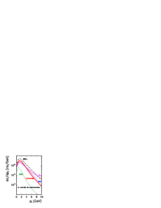
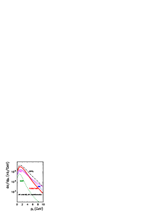
Figure 5: Inclusive $d\sigma/dp_{t}$ for charm/anticharm production at W = 1.96 TeV for different UGDFs. The meaning of the curves is as follows: solid - Kwieciński, thick dashed - KL, thin dashed - GBW, dash-dotted - BFKL, dotted - KMR.

In Fig.5 we collected results obtained with different unintegrated gluon distributions from the literature. In this case consequently the off-shell matrix element and off-shell kinematics were used. The GBW gluon distribution leads to much smaller cross section. The KL gluon distribution produces the hardest $p_{t}$ spectrum. Rather different slopes in transverse momentum of $c$ (or $\bar{c}$) are obtained for different UGDFs. This differences survive after convoluting the inclusive quark/antiquark spectra with fragmentation functions. Thus, in principle, precise distribution in transverse momentum of charmed mesons should be useful to select a “correct” model of UGDF. A detailed comparison with the experimental data requires, however, a detailed knoweledge of fragmentation functions.

The inclusive spectra are not the best observables to test UGDF [1]. Let us come now to correlations between charm quark and charm antiquark.

The azimuthal angle correlation is the most popular observable in this context. There is a trivial relation between the relative azimuthal angle distribution and the average transverse momenta of gluons. This is illustrated in Fig.6 for the simple Gaussian smearing with different values of the parameter $\sigma_{0}$ . In general, the larger $\sigma_{0}$ the more decorrelation can be observed. In the literature both on-shell (see e.g.[3]) and off-shell (see e.g.[4, 5]) kinematics is used. Our calculation shows that there is almost no difference whether on-shell or off-shell kinematics is applied. In Fig.7 we show the angular correlations for the Kwieciński UGDF for different values of the $b_{0}$ parameter. The effect here is smaller than for the simple Gaussian smearing. This is due to the fact that here the perturbative broadening is included explicitly and the parameter $b_{0}$ takes into account only nonperturbative part. The use of on-shell matrix elements instead of off-shell ones leads to slightly stronger back-to-back correlations.

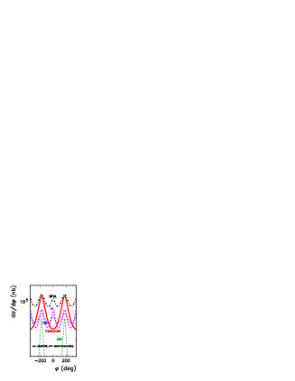
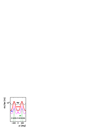
Figure 8: Azimuthal angle correlations for different UGDF in the literature: Kwieciński (solid), BFKL (dash-dotted), GBW (thin dashed), KL (thick dashed) and KMR (dotted).

In Fig.8 we compare results for different unintegrated gluon distribution from the literature. Quite different results are obtained for different UGDF. The nonperturbative GBW glue leads to strong azimuthal correlations between $c$ and $\bar{c}$. In contrast, BFKL dynamics leads to strong decorrelations of azimuthal angles of charm and anticharm quarks. The saturation-idea inspired KL distribution, as well as BFKL and KMR distributions lead to an local enhancement for $\phi_{c\bar{c}}\approx$ 0 which is probably due to gluon splitting s-channel subprocess. In the last case there is a sizeable difference between the result obtained with on-shell (left panel) and off-shell (right panel) matrix elements. Gluon distribution obtained by the KMR method and the KL and BFKL distributions generate very similar shapes in azimuthal angle. The gluon distribution obtained by the solution of the Kwieciński equation gives somewhat narrower distribution around $\phi=\pm\pi$.

The initial state gluon transverse momentum is also responsible for the decorrelation of the charm quark, charm antiquark transverse momenta. In the case of absence of any gluon transverse momenta in leading-order collinear approximation $p_{1,t}=p_{2,t}$. The effect of transverse momenta is shown in Fig.9 for different unintegrated gluon distributions from the literature. Although the main strength is concentrated along the diagonal $p_{1,t}=p_{2,t}$, there is a smearing over whole two-dimensional space of $p_{1,t}\times p_{2,t}$. As for the case of azimuthal correlations, different pattern can be observed for different UGDF.

In general, the shape of the two-dimensional map is governed by the UGDF used and the matrix element squared. It is of interest to unfold these two effects. In Fig.10 we show an average matrix element squared (obtained with the help of BFKL UGDF) in the $p_{1,t}\times p_{2,t}$ space. A rather weak dependence can be observed which means that UGDF is the crucial element responsible for the variation of the cross section in the $p_{1,t}\times p_{2,t}$ space. We compare the on-shell (left panel) and off-shell (right panel) matrix elements squared averaged with UGDF over the phase space. In contrast to the more inclusive cases considered above, here the difference is quite sizeable. In Fig.11 we present the corresponding ratio of both two-dimensional functions.

What is the origin of populating the asymmetric final state configurations? The regions $p_{1,t}\gg p_{2,t}$ and $p_{1,t}\ll p_{2,t}$ are populated by asymmetric initial configurations $\kappa_{1,t}^{2}\gg\kappa_{2,t}^{2}$ or $\kappa_{1,t}^{2}\ll\kappa_{2,t}^{2}$. This is demonstrated in Fig.12 where we show average value of $\kappa_{1,t}^{2}$ and $\kappa_{2,t}^{2}$ obtained for example with KMR gluon distributions. The smallest values of $\kappa_{1,t}^{2}$ and $\kappa_{2,t}^{2}$ are obtained along the diagonal ($p_{1,t}=p_{2,t}$). This means that along diagonal the soft nonperturbative part of UGDF is tested. The larger distance from the diagonal, the larger $\kappa_{1,t}^{2}$ and $\kappa_{2,t}^{2}$ are sampled. The KMR is known to have long tails in gluon transverse momenta. This in conjuction with Fig.12 implies relatively large cross section for $p_{1,t}\gg p_{2,t}$ or $p_{1,t}\ll p_{2,t}$.

In Fig.13 we show two-dimensional maps in $p_{1,t}$ and $p_{2,t}$ obtained for four different complementary regions of $\kappa_{1,t}^{2}$ and $\kappa_{2,t}^{2}$:
(a) $\kappa_{1,t}^{2}<$ 10 GeV², $\kappa_{2,t}^{2}<$ 10 GeV²,
(b) $\kappa_{1,t}^{2}<$ 10 GeV², $\kappa_{2,t}^{2}>$ 10 GeV²,
(c) $\kappa_{1,t}^{2}>$ 10 GeV², $\kappa_{2,t}^{2}<$ 10 GeV²,
(d) $\kappa_{1,t}^{2}>$ 10 GeV², $\kappa_{2,t}^{2}>$ 10 GeV².
The asymmetric (in gluon transverse momentum) configurations contribute a large fraction to the integrated cross section. In Table 1 we ensambled fractions of different regions of $\kappa_{1}^{2}\times\kappa_{2}^{2}$. For completeness we placed in the table the integrated cross section for the $c\bar{c}$ pair production. The KMR and KL have largest fractions of asymmetric initial state configurations. The almost vanishing fraction of asymmetric configurations for GBW glue is due to a lack of pQCD effects. A rather schematic KL distribution includes the hard components only in a simple parametric form. Our purely model discussion here is a bit academic because initial state configurations are not directly the observables. Therefore the effect of the large tails in UGDFs can be only tested indirectly by studying asymmetric configurations in the final state (charmed mesons, muons) space $p_{1,t}\times p_{2,t}$.

The decorrelation in $p_{1,t}$ and $p_{2,t}$ can be also studied in the collinear next-to-leading order approach. It is worth to stress here, however, that collinear approach even in higher order approximation is unreliable in the region $p_{1,t}\approx p_{2,t}$. In order to avoid conceptual and/or numerical problems asymmetric cuts on jets transverse momentum are usually assumed. On experimental side this means removing a big portion of statistics from the correlation studies. Our approach is free of the mentioned above problems and can be applied on the whole plane $p_{1,t}\times p_{2,t}$.

In principle, there are many more correlation observables possible having in view quite reach phase space for two particle production. Here we shall concentrate on one more observable – namely the azimuthal angle correlation for different regions of quark-antiquark transverse momenta. In Fig.14 we show such correlations but now with extra conditions on quark-antiquark transverse momenta. Generally, the larger transverse momenta the more back-to-back correlation is observed. The details depend, however, on a particular model of UGDF.

In Fig.15 we show similar correlations for very asymmetric values of $p_{1,t}$ and $p_{2,t}$. In this domain the cross section obtained with BFKL, KL and KMR UGDFs is much larger than the cross section obtained with the Kwieciński UGDF. While the first three UGDFs lead to almost complete decorrelation of $c$ and $\bar{c}$, for the last UGDF we observe clear back-to-back correlations. Furthermore the absolute cross section in the latter cases is much smaller. This distinct difference causes that this observable is very promissing in testing the QCD dynamics.

In order to shed more light on the relation between the $c$/$\bar{c}$ transverse momentum and azimuthal correlations in Fig.16 we show the effect of transverse momentum of $c$ or $\bar{c}$ and relative azimuthal angle on a two-dimensional map $(p_{t},\phi_{-})$, where $p_{t}$ is transverse momentum of either quark or antiquark. The same effect as in Fig.14 is shown now in a continuous way. There is also a technical lesson from the inspection of Fig.16. The figure shows that one needs somewhat more refine integration in $\phi_{-}$ for larger values of $p_{1,t}$ and $p_{2,t}$.

In the present exploratory calculation we have studied correlations between charm quark and charm antiquark. In practice one measures either muons or charmed mesons. It seems that a study of $p_{t}(D^{*+})\times p_{t}(D^{*-})$ or $p_{t}(\mu^{+})\times p_{t}(\mu^{-})$ or mixed $p_{t}(D^{*+})\times p_{t}(\mu^{-})$ or $p_{t}(\mu^{+})\times p_{t}(D^{*-})$ correlations would be optimal to test UGDFs. This will be a subject of our next studies. It is not clear to us if such measurements are feasible with the present Tevatron apparatus.

5 Conclusions

We have compared quantitatively different methods to include gluon transverse momenta and their effect on inclusive spectra as well as on $c\bar{c}$ correlations. Different UGDFs from the literature were used.

The gluon-gluon luminosity factor is more strongly varying factor over the phase space than the matrix element squared. Consequently, the shape of inclusive spectra only weakly depends on whether on-shell or off-shell matrix element is used. In contrast there is a sizeable effect for more exclusive variables, dependent e.g. on the position in the $p_{1,t}\times p_{2,t}$ space.

We have shown that the analysis of azimuthal correlations and decorrelations on the $p_{1,t}$(c transverse momentum) x $p_{2,t}$($\bar{c}$ transverse momentum) plane as well as the combination of both are very promissing to verify UGDF. We have focussed on the region of $p_{1,t}\gg p_{2,t}$ and $p_{1,t}\ll p_{2,t}$. There max$\{\kappa_{1,t},\kappa_{2,t}\}\sim$ max$\{p_{1,t},p_{2,t}\}$ and off-shell matrix element must be used. In this region the shape of azimuthal correlation function depends on both UGDF and matrix element.

Although we have calculated correlation observables for charm quarks and antiquarks it is obvious that the main effects should be very similar for charmed mesons and/or muons. The correlations between $D^{*+}(c\bar{d})$ and $D^{*-}(\bar{c}d)$ or $\mu^{+}$ and $\mu^{-}$ are the most promissing in this respect as they reflect relatively well the $c\bar{c}$ final state. Estimating the rates of events with one $D$ meson with small transverse momentum and second $D$ meson with large transverse momentum would be a useful test of the QCD dynamics. The analysis of meson correlations will be a subject of our next analysis.

Acknowledgements We are indebted to Sergey Baranov for an interesting discussion on heavy quark - heavy antiquark correlations. This work was partially supported by the grant of the Polish Ministry of Scientific Research and Information Technology number 1 P03B 028 28.

TABLES

Table 1: Fractions in % of contributions from different regions of $\kappa_{1}^{2}\times\kappa_{2}^{2}$ to the total cross section for different UGDFs from the literature for W = 1.96 TeV, with off-shell kinematics and off-shell matrix elements. In the case of Kwieciński UGDF: $b_{0}$ = 1 GeV^-1, $\mu_{F}^{2}$ = 4 $m_{c}^{2}$, in the case of KMR UGDF: $\mu_{F}^{2}$ = 4 $m_{c}^{2}$. Below for brevity $\xi^{2}$ = 10 GeV² is assumed.

UGDF	$\sigma_{c\bar{c}}^{tot}$(mb)	$\kappa_{1}^{2}<\xi^{2},\kappa_{2}^{2}<\xi^{2}$	$\kappa_{1}^{2}<\xi^{2},\kappa_{2}^{2}>\xi^{2}$	$\kappa_{1}^{2}>\xi^{2},\kappa_{2}^{2}<\xi^{2}$	$\kappa_{1}^{2}>\xi^{2},\kappa_{2}^{2}>\xi^{2}$
Kwieciński	0.85	91.87	3.99	3.99	0.15
KMR	0.55	52.43	19.83	19.83	7.91
BFKL	1.44	59.65	17.26	17.26	5.83
GBW	0.12	100.0	0.001	0.001	0.0
KL	0.51	65.49	15.37	15.37	3.76

FIGURES

Figure 1: Inclusive $d\sigma/dp_{t}$ for charm/anticharm production at W = 1.96 TeV in the approach of naive Gaussian smearing of gluon transverse momenta. The calculation with different values of $\sigma_{0}=$ 0.25 (dotted), 0.50 (dashed), 1.0 (solid), 2.0 (dash-dotted) GeV are shown. The results with on-shell kinematics are shown in panel (a) and results with off-shell kinematics in panel (b). In this calculation both factorization and renormalization scales were fixed for 4 $m_{c}^{2}$.

Figure 2: Inclusive $d\sigma/dp_{t}$ for charm/anticharm production at W = 1.96 TeV for the Kwieciński unintegrated gluon distributions for $b_{0}=$ 0.5, 1.0, 2.0 GeV^-1 and for $\mu_{F}^{2}=4m_{c}^{2}$. The results with on-shell matrix element is shown in the left panel and results with off-shell matrix element in the right panel.

Figure 3: Inclusive $d\sigma/dp_{t}$ for charm/anticharm production at W = 1.96 TeV for the Kwieciński UGDF for different factorization scales $\mu_{F}^{2}$ = $m_{c}^{2}$ (dashed), 4 $m_{c}^{2}$ (solid). In this calculation $b_{0}=$ 1.0 GeV^-1.

Figure 4: Inclusive $d\sigma/dp_{t}$ for charm/anticharm production at W = 1.96 TeV for the Kwieciński UGDF for on-shell (dashed) and off-shell (solid) matrix element. In this calculation $b_{0}$ = 1.0 GeV^-1, $\mu_{R}^{2}$ = $\mu_{F}^{2}$ = 4 $m_{c}^{2}$.

Figure 6: Azimuthal angle correlations for different values of the Gaussian parameter $\sigma_{0}$ = 0.25, 0.50, 1.0, 2.0 GeV for on-shell (panel a) and off-shell (panel b) kinematics. Here 0 $<p_{1,t},p_{2,t}<$ 10 GeV.

Figure 7: Azimuthal angle correlations for the Kwieciński UGDF for different values of the parameter $b_{0}$ = 0.5, 1.0, 2.0 GeV^-1. In this calculation $\mu_{R}^{2}$ = $\mu_{F}^{2}$ = 4 $m_{c}^{2}$ was taken.

Figure 9: Two-dimensional distributions in $p_{1,t}$ of charm quark and $p_{2,t}$ of charm antiquark for different UGDF in the literature: (a) KMR ($\mu_{F}^{2}=4m_{c}^{2}$), (b) Kwieciński ($b_{0}$ = 1.0 GeV^-1, $\mu_{F}^{2}=4m_{c}^{2}$), (c) BFKL, (d) KL.

Figure 10: Average matrix element squared as a function of $p_{1,t}$ of charm quark and $p_{2,t}$ of charm antiquark for on-shell (left panel) and off-shell (right panel) matrix element. In this calculation BFKL UGDF was used.

Figure 11: The ratio of the maps (from the previous figure) with off-shell and on-shell matrix elements.

Figure 12: Average transverse momenta of initial gluons $\kappa_{1,t}^{2}$ or $\kappa_{2,t}^{2}$ as a function of $p_{1,t}$ and $p_{2,t}$. In this calculation Kimber-Martin-Ryskin UGDF was used.

Figure 13: Two-dimensional distributions in $p_{1,t}$ of charm quark and $p_{2,t}$ of charm antiquark for the KMR UGDF and for different regions of gluon transverse momenta specified in the text.

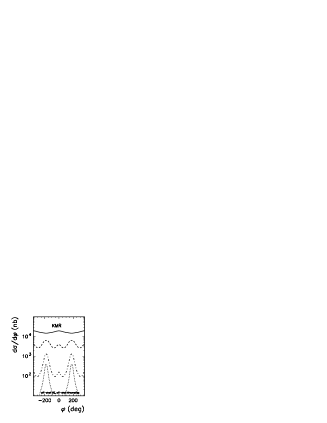
Figure 14: $d\sigma/d\phi_{-}$ for different intervals of charm and anticharm transverse momenta:
0.0 GeV $<p_{1,t},p_{2,t}<$ 2.5 GeV (solid),
2.5 GeV $<p_{1,t},p_{2,t}<$ 5.0 GeV (dashed),
5.0 GeV $<p_{1,t},p_{2,t}<$ 7.5 GeV (dash-dotted),
7.5 GeV $<p_{1,t},p_{2,t}<$ 10.0 GeV (dotted)
for different UGDF: (a) KMR ($\mu^{2}=4m_{c}^{2}$), (b) Kwieciński ($b_{0}$ = 0.5 GeV^-1, $\mu^{2}=4m_{c}^{2}$), (c) BFKL, (d) KL.

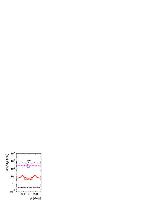
Figure 15: $d\sigma/d\phi_{-}$ for
0.0 GeV $<p_{1,t}<$ 2.5 GeV and 7.5 GeV $<p_{2,t}<$ 10. GeV or
7.5 GeV $<p_{1,t}<$ 10. GeV and 0.0 GeV $<p_{2,t}<$ 2.5 GeV
for different UGDF: KMR ($\mu_{F}^{2}=4m_{c}^{2}$) – dotted, Kwieciński ($b_{0}$ = 0.5 GeV^-1, $\mu_{F}^{2}=4m_{c}^{2}$) – solid, BFKL – dash-dotted, and KL – dashed.

Figure 16: $d\sigma/dp_{t}d\phi_{-}$ for different UGDF: (a) KMR ($\mu_{F}^{2}=4m_{c}^{2}$), (b) Kwieciński ($b_{0}$ = 0.5 GeV^-1, $\mu_{F}^{2}=4m_{c}^{2}$), (c) BFKL, (d) KL.

References

- [1] M. Łuszczak and A. Szczurek, Phys. Lett. B594 (2004) 291.
-
[2]
J.F. Owens, Rev. Mod. Phys. 59 (1987) 465;
Ch-Y. Wong and H. Wang, Phys. Rev. C58 (1998) 376.;
Y. Zhang, G. Fai, G. Papp, G.G. Barnaföldi and P. Lévai, Phys. Rev. C65 (2002) 034903. - [3] U. d’Alesio and F. Murgia, Phys. Rev. D70 (2004) 074009.
- [4] S. Catani, M. Ciafaloni and F. Hautmann, Nucl. Phys. 366 (1991) 135.
- [5] J.C. Collins and R.K. Ellis, Nucl. Phys. B360 (1991) 3.
- [6] R.D. Ball and R.K. Ellis, J.H.E.P. 0105 (2001) 053.
-
[7]
E.M. Levin, M.G. Ryskin, Yu.M. Shabelski and A.G. Shuvaev,
Sov. J. Nucl. Phys. 53 (1991) 657;
M.G. Ryskin, Yu.M. Shabelski and A.G. Shuvaev, Z. Phys. C69 (1996) 269;
Yu.M. Shabelski and A.G. Shuvaev, Eur. Phys. J. C6 (1999) 313;
M.G. Ryskin, A.G. Shuvaev and Yu.M. Shabelski, Phys. Atom. Nucl. 64 (2001) 1995; Yu.M. Shabelski and A.G. Shuvaev, hep-ph/0107106; Yu.M. Shabelski and A.G. Shuvaev, hep-ph/0406157. - [8] S.P. Baranov and M. Smizanska, Phys. Rev. D62 (2000) 014012.
-
[9]
A.V. Lipatov, V.A. Saleev and N.P. Zotov, hep-ph/0112114;
S.P. Baranov, A.V. Lipatov and N.P. Zotov, hep-ph/0302171, Yad. Fiz. 67 (2004) 856. - [10] V.D. Barger and R.J.N. Phillips, “Collider physics”, Addison-Wesley Publishing Company, 1987
- [11] J. Kwieciński, Acta Phys. Polon. B33 (2002) 1809.
- [12] A. Gawron and J. Kwieciński, Acta Phys. Polon. B34 (2003) 133.
- [13] A. Gawron, J. Kwieciński and W. Broniowski, Phys. Rev. D68 (2003) 054001.
- [14] J. Kwieciński and A. Szczurek, Nucl. Phys. B680 (2004) 164.
-
[15]
M. Czech and A. Szczurek, Phys. Rev. C72 (2005) 01502;
M. Czech and A. Szczurek, nucl-th/050910007. - [16] A. Szczurek, Acta Phys. Polon. B34 (2003) 3191.
-
[17]
M.A. Kimber, A.D. Martin and M.G. Ryskin,
Eur. Phys. J. C12 (2000) 655;
M.A. Kimber, A.D. Martin and M.G. Ryskin, Phys. Rev. D63 (2001) 114027-1. - [18] J. Kwieciński, A.D. Martin and A. Staśto, Phys. Rev. D56 (1997) 3991.
-
[19]
E.A. Kuraev, L.N. Lipatov and V.S. Fadin,
Sov. Phys. JETP 45 (1977) 199;
Ya.Ya. Balitskij and L.N. Lipatov, Sov. J. Nucl. Phys. 28 (1978) 822. - [20] A.J. Askew, J. Kwieciński, A.D. Martin and P.J. Sutton, Phys. Rev. D49 (1994) 4402.
- [21] K.J. Eskola, A.V. Leonidov and P.V. Ruuskanen, Nucl. Phys. B481 (1996) 704.
- [22] K. Golec-Biernat and M. Wüsthoff, Phys. Rev. D60 (1999) 114023-1.
- [23] D. Kharzeev and E. Levin, Phys. Lett. B523 (2001) 79.
- [24] M. Glück, E. Reya and A. Vogt, Z. Phys. C67 (1995) 433.
- [25] M. Glück, E. Reya and A. Vogt, Eur. Phys. J. C5 (1998) 461.