Twistor String Theory and QCD

Abstract

I review recent progress in using twistor-inspired methods to compute perturbative scattering amplitudes in gauge theory, for application to collider physics.

1 Introduction

In two years, a new window will open into physics at the shortest distance scales. The Large Hadron Collider (LHC) will begin operation at CERN, providing proton-proton collisions at 14 TeV center-of-mass energy, seven times greater than the 2 TeV currently available in $p\bar{p}$ collisions at Fermilab’s Tevatron. The LHC luminosity should be a factor of 10 to 100 greater than the Tevatron’s. The combined rise in energy and luminosity will lead to a huge increase in the production of particles with masses in the range 100–1000 GeV, including electroweak vector bosons, top quarks, Higgs bosons, and of course new particles, representing physics beyond the Standard Model.

There are a lot of ideas for physics beyond the Standard Model, many associated with the puzzle of electroweak symmetry breaking, and with resolutions of the hierarchy problem — why the weak scale is so much smaller than the Planck scale. Supersymmetry, for example, predicts a host of new particles in the 100–1000 GeV mass range, including (in most versions) a stable dark matter candidate. However, many other theories — new dimensions of space-time, new forces, etc. — often make qualitatively similar predictions. How can we sort out the predictions of these theories from each other, and from the omnipresent Standard Model background at a hadron collider?

The short answer is that a thorough, quantitative understanding of both the new physics signals and the Standard Model backgrounds is required. Much work has gone into these problems, stretching back over many decades. This talk will focus on some recent developments, novel methods to help compute the backgrounds in particular, that have emerged since the Fall of 2003, when Witten introduced twistor string theory and explained its relevance to perturbative QCD WittenTopologicalString . In truth, the new methods have not yet had a direct phenomenological impact, in terms of producing more accurate cross sections that have not previously been obtained in any other way. But they have a lot of promise, and it should not be long before they do so.

What are some generic properties of the new physics signals? Except for stable, neutral dark matter candidates, the new massive particles typically decay into “old” Standard Model particles: quarks, gluons, charged leptons and neutrinos, photons, $W$s and $Z$s. For example, in supersymmetry the superpartner of the gluon, the gluino, may be among the heavier superparticles, yet still be copiously produced at the LHC, due to its large adjoint color charge. Figure 1 shows a typical decay cascade, initiated by one of the two gluinos ($\tilde{g}$) in a pair-production event. The quarks and gluons emerge as jets of hadrons. The lightest superpartner, a neutralino ($\chi^{0}$), is stable and escapes the detector. The kinematic signatures of such events are not always clean: There can be a large number of observed particles (charged leptons or jets), and no invariant-mass bumps, because of the escaping neutralinos and possibly neutrinos (although there can be kinematic edges). The escaping neutralinos provide a missing transverse energy signal, but Standard Model production of $Z$ bosons, followed by $Z$ decays to neutrinos, can mimic this to some degree.

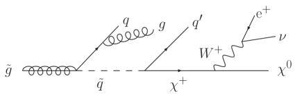
Figure 1: Typical cascade decay of a gluino to two quarks, a gluon, a $W$ boson which decays to two leptons, and a neutralino. Aside from the neutralino, all the final-state particles are essentially massless.

In order to maximize the potential for the discovery and interpretation of new physics at the LHC, we need to quantify the Standard Model backgrounds for processes that may contain several jets and (perhaps) a few electroweak bosons. These processes are complex, so we should try to take into account any simplifying features. Notice that the masses of the observed final-state particles in these reactions (e.g. in fig. 1) are generally negligibly small in these reactions, except for the cases of the $W$, $Z$, or top quark. Even these particles immediately decay to essentially massless quarks or leptons, however. So if we include the decay processes in the description of the event, every final-state particle is approximately massless. We can also (usually) neglect the masses of the colliding partons (quarks and gluons). In general, then, the backgrounds (and many signals) require a detailed understanding of scattering amplitudes for many ultra-relativistic (massless) particles – especially the quarks and gluons of QCD.

Asymptotic freedom GWP allows us to compute such scattering amplitudes as a perturbative expansion in the strong coupling constant $\alpha_{s}(\mu)$, evaluated at a large momentum scale $\mu$ where it is small. For typical collider processes, $\mu$ could be of order 100–200 GeV, for which $\alpha_{s}(\mu)\approx 0.1$. One might expect that the leading-order terms in the expansion (tree amplitudes) would suffice to get a 10% uncertainty. However, this is not the case for hadron collider cross sections; typical corrections from the next-to-leading order (NLO) terms in the $\alpha_{s}$ expansion are 30% to 100%. There are several possible reasons for the large corrections, depending on the process: there may be different scales involved, leading to large logarithms of the ratio(s) of scales; new partonic subprocesses may first arise at NLO; the lowest-order process may have several factors of $\alpha_{s}$ in it; and so on. In any event, a quantitative description of collider events requires evaluation of cross sections at NLO in QCD, which in turn requires, as input, one-loop amplitudes as well as tree amplitudes. If a precise evaluation is needed (below 10% uncertainty), then the next-to-next-to-leading order terms, involving two-loop amplitudes, may also be required.

In principle, Feynman rules FeynPT are all we need to evaluate the tree and loop amplitudes. In practice, however, although Feynman rules are very general, applying to any local quantum field theory, by the same token they are not optimized for the problems at hand. More efficient methods are available, which make use of the extra symmetries (some hidden) of QCD.

2 Transforming to twistor space

An easy way to see that there should be more efficient methods out there is to notice that many QCD amplitudes are much simpler than expected. For example, the tree-level amplitudes for the scattering of $n$ gluons turn out to all vanish, if the helicities of the gluons (considered as outgoing particles) are either a) all the same, or b) all the same, except for one of opposite helicity. Using parity, we can take the bulk of the gluons to have positive helicity, and write this vanishing relation as

$$A_{n}^{\rm tree}(1^{\pm},2^{+},3^{+},\ldots,n^{+})=0\,.$$ (1)

This vanishing is somewhat mysterious from the point of view of Feynman diagrams. On the other hand, it can be demonstrated simply using Ward identities arising from a secret supersymmetry that tree-level QCD amplitudes possess SWI . This symmetry allows two of the gluons to be replaced by their superpartners, gluinos, which can be taken to be massless here. Helicity conservation for the gluinos then implies the vanishing of the amplitudes.

The first sequence of nonvanishing tree amplitudes has two gluons with negative helicity, labelled by $j$ and $l$, say, and the rest of positive helicity. This sequence of maximally helicity-violating (MHV) amplitudes has an exceedingly simple form ParkeTaylor ; BGSixMPX ,

$$A_{n}^{{\rm MHV}\,,jl}\equiv A_{n}^{\rm tree}(1^{+},2^{+},\ldots,j^{-},\ldots,l^{-},\ldots,n^{+})=i{{\left\langle j\,l\right\rangle}^{4}\over\left\langle 1\,2\right\rangle\left\langle 2\,3\right\rangle\cdots\left\langle n\,1\right\rangle}\,,$$ (2)

in terms of spinor products $\left\langle i\,j\right\rangle$ we shall define shortly. Equation (2) is the expression for, not the full amplitude, but rather a piece of it where the $n$ gluons have a definite cyclic ordering. The full amplitude can be built out of permutations of such partial amplitudes, as reviewed for example in ref. TreeReview . Some of the structure of eq. (2) follows from supersymmetry, but not all.

To see much more of the structure, Witten WittenTopologicalString transformed the amplitudes (2) from the traditional momentum-space variables, into a twistor space invented by Penrose Penrose . The twistor transform is a kind of Fourier transform. There are many examples where transforming a problem into the right variables can expose its simplicity. For example, if we measure the time dependence of the electric field $E(t)$ associated with the light emerging from some glowing sample of gas, we find a fairly unenlightening waveform. However, if we use a spectrometer to measure instead the frequency (energy) spectrum of the light, that is, $E(\omega)=\int dte^{i\omega t}E(t)$, we find spectral lines, which are clues toward decoding the structure of the emitting gas. In in an analogous way, the twistor transform exposes certain lines on which QCD amplitudes are localized or supported, thus revealing more of their structure, and giving rise to new, more efficient ways to compute them.

Before describing the twistor transform, however, we should discuss the spinor variables used in eq. (2), because they are well-suited for describing scattering amplitudes for massless particles with spin, and are the starting point for the twistor transform. Let $i=1,2,\ldots,n$ label the particles being scattered. Usually, the four-momentum vectors $k_{i}^{\mu}$, which transform under the spin-1 representation of the Lorentz group, are used as the arguments of the amplitude, $A=A(k_{i})$. The relativistic invariants constructed out of these vectors are the Lorentz inner products, or invariant masses, $s_{ij}=2k_{i}\cdot k_{j}=(k_{i}+k_{j})^{2}$, which are equivalent in the massless case, $k_{i}^{2}=0$. However, for massless particles with spin, it is better to “take the square root” and use, instead of $k_{i}^{\mu}$, objects transforming as the spin-1/2 representation of the Lorentz group, namely the massless Dirac spinors associated with momentum $k_{i}$, $u_{\pm}(k_{i})$, where the $\pm$ sign labels the helicity. A shorthand notation for the two-component (Weyl) versions of these spinors is,

$$(\lambda_{i})_{\alpha}\equiv\bigl{[}u_{+}(k_{i})\bigr{]}_{\alpha},\qquad({\tilde{\lambda}}_{i})_{\dot{\alpha}}\equiv\bigl{[}u_{-}(k_{i})\bigr{]}_{\dot{\alpha}}.$$ (3)

We can always reconstruct the momenta from the spinors, using the positive-energy projector for massless spinors, $u(k)\bar{u}(k)={\raise 0.97221pt\hbox to5.52084pt{\hss/\hss}\hbox to0.0pt{\hss$k$}}$, or in two-component notation,

$$k_{i}^{\mu}(\sigma_{\mu})_{\alpha\dot{\alpha}}=({\raise 0.97221pt\hbox to5.52084pt{\hss/\hss}\hbox to0.0pt{\hss$k$}}_{i})_{\alpha\dot{\alpha}}=(\lambda_{i})_{\alpha}({\tilde{\lambda}}_{i})_{\dot{\alpha}}\,.$$ (4)

Equation (4) shows that a massless momentum vector, written as a bi-spinor, is the product of a left-handed spinor with a right-handed one.

Instead of Lorentz inner products of momenta, $s_{ij}=2k_{i}\cdot k_{j}$, we use spinor products, defined by

$$\left\langle j\,l\right\rangle=\varepsilon^{\alpha\beta}(\lambda_{j})_{\alpha}(\lambda_{l})_{\beta}=\bar{u}_{-}(k_{j})u_{+}(k_{l})\,,\qquad\left[j\,l\right]=\varepsilon^{\dot{\alpha}\dot{\beta}}({\tilde{\lambda}}_{j})_{\dot{\alpha}}({\tilde{\lambda}}_{l})_{\dot{\beta}}=\bar{u}_{+}(k_{j})u_{-}(k_{l})\,,$$ (5)

where $\varepsilon^{\alpha\beta}$ and $\varepsilon^{\dot{\alpha}\dot{\beta}}$ are antisymmetric tensors for $SU(2)$. These products satisfy

$$\left\langle i\,j\right\rangle\left[j\,i\right]={1\over 2}{\rm Tr}[{\raise 0.97221pt\hbox to5.52084pt{\hss/\hss}\hbox to0.0pt{\hss$k$}}_{i}{\raise 0.97221pt\hbox to5.52084pt{\hss/\hss}\hbox to0.0pt{\hss$k$}}_{j}]=2k_{i}\cdot k_{j}=s_{ij}\,.$$ (6)

So they are just the square roots of the Lorentz inner products, up to a phase $\phi$,

$$\left\langle j\,l\right\rangle=\sqrt{s_{jl}}e^{i\phi_{jl}}\,,\qquad\left[j\,l\right]=\pm\sqrt{s_{jl}}e^{-i\phi_{jl}}\,.$$ (7)

The utility of spinor variables for QCD amplitudes was recognized already in the 1980s SpinorHelicity ; BGSixMPX . They precisely capture the “square-root-plus-phase” behavior of gauge theory amplitudes as the momenta of two of the particles, $i$ and $j$, become collinear. This behavior arises because the sum of the helicities of the final-state particles is never equal to the helicity of the almost-on-shell intermediate particle, as illustrated in fig. 2(b) for the case of a gluon splitting into two gluons, for which $\pm 1\pm 1\neq\pm 1$. This mismatch in angular momentum along the collinear direction lessens the singularity, from $1/s_{ij}$ (the behavior of the scalar theory shown in fig. 2(a)) to $1/\sqrt{s_{ij}}$. It also introduces a phase depending on the azimuthal angle, which is conjugate to the angular momentum. Equation (7) shows that both characteristics are captured by putting a spinor product in the denominator of the amplitude, explaining why the spinor products are natural variables to use. In other words, we should write $A=A(\lambda_{i},{\tilde{\lambda}}_{i})$ instead of $A=A(k_{i})$.

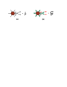
Figure 2: Contrasting collinear behavior of amplitudes in (a) massless scalar $\phi^{3}$ theory, where there is no angular-momentum mismatch, and (b) massless gauge theory, for example a gluon splitting into two gluons, where there is always a mismatch.

Now we can describe the twistor transform Penrose ; WittenTopologicalString . It is a “half” Fourier transform, in which the right-handed spinors $\lambda_{i}$ are left untouched, but each left-handed spinor ${\tilde{\lambda}}_{i}$ is exchanged for its Fourier conjugate variable $\mu_{i}$, defined by

$${\tilde{\lambda}}_{\dot{\alpha}}=i{\partial\over\partial\mu^{\dot{\alpha}}}\,,\qquad\mu^{\dot{\alpha}}=i{\partial\over\partial{\tilde{\lambda}}_{\dot{\alpha}}}\,.$$ (8)

(These relations are completely analogous to the standard Fourier relation between momentum and position, $x=i\partial/\partial p$, $p=-i\partial/\partial x$.) Since the spinors and their conjugates each have two components, twistor space has four coordinates (for each external particle), $(\lambda_{1},\lambda_{2},\mu^{\dot{1}},\mu^{\dot{2}})$. However, because amplitudes are only defined up to a phase associated with external states, two points in twistor space are equivalent if the four coordinates differ by a constant multiple $\xi$ (the complexification of the phase),

$$(\lambda_{1},\lambda_{2},\mu^{\dot{1}},\mu^{\dot{2}})\equiv(\xi\lambda_{1},\xi\lambda_{2},\xi\mu^{\dot{1}},\xi\mu^{\dot{2}}).$$ (9)

So in fact (projective) twistor space is three-dimensional.

What do amplitudes look like in this space? We can compute them by Fourier transforming, just as we would to take a wave-function from position-space to momentum-space WittenTopologicalString ,

$$A(\lambda_{i},{\tilde{\lambda}}_{i})\quad\Rightarrow\quad A(\lambda_{i},\mu_{i})\equiv\int\prod_{i=1}^{n}d{\tilde{\lambda}}_{i}\,e^{i\mu_{i}{\tilde{\lambda}}_{i}}A(\lambda_{i},{\tilde{\lambda}}_{i})\,.$$ (10)

The simplest cases to consider are the MHV amplitudes (2), which contain only angle brackets ($\left\langle i\,j\right\rangle$), and so depend almost exclusively on the right-handed spinors $\lambda_{i}$, $A_{n}^{\rm MHV}(\lambda_{i},{\tilde{\lambda}}_{i})\equiv A_{n}^{\rm MHV}(\lambda_{i})$. Their only dependence on the left-handed spinors is through the usual momentum-conserving $\delta$-function (which was implicit in eq. (2)). This factor can be written, using the identity

$$\delta^{4}(k)=\int d^{4}x\,\exp[ik\cdot x]$$ (11)

and eq. (4), as

$$\delta^{4}\Bigl{(}\sum_{i=1}^{n}k_{i}\Bigr{)}=\int d^{4}x\,\exp\Bigl{[}ix^{\alpha\dot{\alpha}}\sum_{i=1}^{n}(\lambda_{i})_{\alpha}({\tilde{\lambda}}_{i})_{\dot{\alpha}}\Bigr{]}\,.$$ (12)

Then the transformed amplitudes are

$$A_{n}^{{\rm MHV}}(\lambda_{i},\mu_{i}) = \int\prod_{i=1}^{n}d{\tilde{\lambda}}_{i}\exp[i\mu_{i}{\tilde{\lambda}}_{i}]\int d^{4}x\ A_{n}^{{\rm MHV}}(\lambda_{i})\exp[ix\lambda_{i}{\tilde{\lambda}}_{i}]$$ (13)

$$= \int d^{4}x\ A_{n}^{{\rm MHV}}(\lambda_{i})\int\prod_{i=1}^{n}d{\tilde{\lambda}}_{i}\exp[i(\mu_{i}+x\lambda_{i}){\tilde{\lambda}}_{i}]$$

$$= A_{n}^{{\rm MHV}}(\lambda_{i})\int d^{4}x\prod_{i=1}^{n}\delta(\mu_{i}+x\lambda_{i})\,.$$

The product of all the linear $\delta$-function constraints simply means that the amplitude is supported on a line in twistor space, as shown in fig. 3(a).

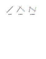
Figure 3: Tree amplitudes for $n$ gluons are supported on networks of intersecting lines in twistor space. The number of lines is one fewer than the number of negative-helicity gluons.

More complicated amplitudes can also be inspected. The first nonvanishing, non-MHV $n$-gluon amplitudes are the six-gluon amplitudes with three positive and three negative helicities, first computed, from 220 Feynman diagrams, in 1988 BGSixMPX . The simplest case, where the three positive helicities are adjacent, is given by,

$$A_{6}^{\rm tree}(1^{+},2^{+},3^{+},4^{-},5^{-},6^{-}) = i\biggl{[}{(\left[1\,2\right]\left\langle 4\,5\right\rangle\left\langle\smash{6}{\vphantom{1}}^{-}\right|{(1+2)}\left|\smash{3}{\vphantom{1}}^{-}\right\rangle)^{2}\over s_{61}s_{12}s_{34}s_{45}s_{612}}$$ (14)

$$\hskip 0.0pt+{(\left[2\,3\right]\left\langle 5\,6\right\rangle\left\langle\smash{4}{\vphantom{1}}^{-}\right|{(2+3)}\left|\smash{1}{\vphantom{1}}^{-}\right\rangle)^{2}\over s_{23}s_{34}s_{56}s_{61}s_{561}}$$

$$\hskip-128.0374pt+{s_{123}\left[1\,2\right]\left[2\,3\right]\left\langle 4\,5\right\rangle\left\langle 5\,6\right\rangle\left\langle\smash{6}{\vphantom{1}}^{-}\right|{(1+2)}\left|\smash{3}{\vphantom{1}}^{-}\right\rangle\left\langle\smash{4}{\vphantom{1}}^{-}\right|{(2+3)}\left|\smash{1}{\vphantom{1}}^{-}\right\rangle\over s_{12}s_{23}s_{34}s_{45}s_{56}s_{61}}\biggr{]}\,.$$

where $s_{abc}\equiv(k_{a}+k_{b}+k_{c})^{2}$ and $\left\langle\smash{a}{\vphantom{1}}^{-}\right|{(b+c)}\left|\smash{d}{\vphantom{1}}^{-}\right\rangle\equiv\bar{u}_{-}(k_{a})({\raise 0.97221pt\hbox to5.52084pt{\hss/\hss}\hbox to0.0pt{\hss$k$}}_{b}+{\raise 0.97221pt\hbox to5.52084pt{\hss/\hss}\hbox to0.0pt{\hss$k$}}_{c})u_{-}(k_{d})$.

The seven-gluon amplitudes were also computed around this time BGKSeven , using off-shell recursive methods BGRecursive to avoid dealing directly with the 2,485 Feynman diagrams. The explicit results in this case fill several pages. Computing the twistor transform via eq. (10) is rather difficult. However, suppose one has a guess for how the amplitudes are supported in twistor space, for example that they are localized on some curve described by a polynomial equation $C(Z_{i})=0$, where $Z=(\lambda_{1},\lambda_{2},\mu^{\dot{1}},\mu^{\dot{2}})$. Then it is relatively easy to check such a guess back in spinor-space, where $C(Z_{i})$ becomes a differential operator, since $\mu_{i}=i\partial/\partial{\tilde{\lambda}}_{i}$. Applying $C(Z_{i})$ to $A(\lambda_{i},{\tilde{\lambda}}_{i})$, if the result vanishes identically then the amplitude is supported on the curve; that is, either $C=0$ or else $A=0$.

This method was used last year by Cachazo, Svrček and Witten WittenTopologicalString ; CSWI ; CSWII to build up evidence for the picture illustrated in fig. 3. Scattering amplitudes for $n$ gluons, of which $n_{-}$ have negative helicity, are localized in twistor space on networks of intersecting lines, where the number of intersecting lines is $n_{-}-1$. The MHV case, $n_{-}=2$, was discussed above. The next-to-MHV (NMHV) amplitudes with $n_{-}=3$, for example the six-gluon example in eq. (14), are sums of terms, each of which is supported on a pair of intersecting lines, as shown in fig. 3(b). The partitioning of points among the lines can vary from term to term. Three intersecting lines are needed to describe the next-to-next-to-MHV (NNMHV) amplitudes with $n_{-}=4$ (fig. 3(c)), and so on.

3 MHV rules

While the twistor structure shown in fig. 3 is extremely appealing, it does not directly yield the numerical values of the amplitudes. However, Cachazo, Svrček and Witten CSWI also wrote down a set of diagrammatic “MHV” rules, which can be used in place of Feynman rules to compute the amplitudes, and which make the twistor structure in fig. 3 manifest. Each MHV diagram generates a term in the amplitude which has one of the possible twistor structures, taking into account the possible partitionings of points among the $(n_{-}-1)$ lines. For example, the MHV diagram in fig. 4, for an amplitude with $n_{-}=4$, corresponds to the twistor structure in fig. 3(c). The helicities of internal, as well as external, gluons are labeled by $\pm$ in the diagram. Each vertex must have exactly two negative-helicity gluons attached to it, but it can have an arbitrary number of positive-helicity gluons, just like the MHV amplitude (2). In fact, the rule for this MHV vertex (the complex number associated with it) is given by eq. (2), with a simple prescription for continuing intermediate legs off shell. The rule for an internal line is a factor of $i/p^{2}$, much like a scalar propagator. For processes with a large number of gluons, there are considerably fewer MHV diagrams than Feynman diagrams, because many Feynman subdiagrams get lumped into single MHV vertices. Also, the algebra required to evaluate each diagram is considerably simpler than for the typical Feynman diagram, because there is no tangle of Lorentz indices to follow.

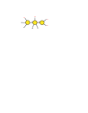
Figure 4: Example of an MHV diagram, corresponding to fig. 3(c).

Because the MHV rules are so efficient, they were quickly generalized to a more general set of processes of interest in the context of LHC signals and backgrounds: tree-level QCD amplitudes containing massless external fermions as well as gluons ExtFerm ; those with a Higgs boson, which couples to gluons via $H{\rm Tr}(G_{\mu\nu}G^{\mu\nu})$ in the large $m_{t}$ limit ExtHiggs ; and amplitudes including one or more electroweak vector bosons in addition to massless quarks and gluons ExtVector . A set of scalar-type rules for QCD with massive quarks (e.g. the top quark) was also produced, starting directly from the QCD Lagrangian SchwinnWeinzierl .

4 Twistor structure at one loop

In parallel with the extension of tree-level MHV rules to different processes, the twistor structure of one-loop amplitudes began to be investigated CSWII . For multi-particle processes, one-loop amplitudes are much more intricate than tree amplitudes. Their twistor structure is also complicated by a “holomorphic anomaly” HoloAnomaly , in which derivatives from $\mu_{i}=i\partial/\partial{\tilde{\lambda}}_{i}$ act near singular regions of the loop integration. For these reasons, it has proven simpler to proceed by first representing amplitudes as linear combinations of various types of basic one-loop integrals — boxes, triangles, bubbles, etc. — and then examining the twistor structure of the coefficients of these integrals.

The simplest situation to consider is a “toy model” for perturbative QCD, namely its maximally supersymmetric cousin, ${\cal N}=4$ super-Yang-Mills theory. In this theory, the coefficients of the triangle and bubble integrals all vanish, reducing the problem to that of determining the coefficients of box integrals Neq4MHV . These coefficients can be found quite readily HoloAnomaly ; NMHVSeven ; BCFGenUnitarity ; Neq4NMHV by inspecting either standard two-particle unitarity cuts Cutting ; Neq4MHV ; LoopReview , or (more efficiently) generalized cuts ELOP ; Zqggq where four propagators are held open BCFGenUnitarity .

The resulting twistor structure NMHVSeven ; Neq4NMHV ; BCFCoplanarity is illustrated in fig. 5. In the MHV case shown in fig. 5(a), the only nonvanishing box coefficients are those where two of the external momenta for the scattering amplitude, $s_{1}$ and $s_{2}$, are also momenta for the box integral; the remaining external momenta are partitioned into two diagonally opposite clusters, $A$ and $B$. This integral is referred to as a two-mass box, because the clustered momenta $K_{A}=\sum_{i\in A}k_{i}$ and $K_{B}=\sum_{i\in B}k_{i}$ are massive, $K^{2}_{A,B}\neq 0$. The coefficient of the two-mass box Neq4MHV is just the MHV tree amplitude (2), which is localized on a single line in twistor space (see fig. 3(a)). In fig. 5(a), the single line has been redrawn as a pair of lines intersecting in two points, $s_{1}$ and $s_{2}$, to make its appearance consistent with an “MHV rules” approach to one-loop amplitudes BST , and with the pattern found for more negative-helicity gluons. (Just as in Euclidean space, a pair of straight lines intersecting in two points in twistor space is the same as a single line.) In the NMHV case shown in fig. 5(b), the simplest nonvanishing box coefficients are generically those of the three-mass box integral, for which three of the legs, $A$, $B$, and $C$, represent clusters of momenta from the scattering amplitude, and only one, $s$, is an individual scattering momentum. These coefficients have a planar twistor structure, consisting of three intersecting lines, and the leg $s$ sits at one of the intersections NMHVSeven ; BCFCoplanarity ; Neq4NMHV . For the NNMHV case in fig. 5(c), the four-mass box coefficients have the nonplanar ring structure shown Neq4NMHV . In general, as in the tree case, fig. 3, one-loop box coefficients are supported on networks of lines, but the lines are joined into rings to match the loop topology. Similar structures have been found for coefficients of integrals in gauge theories with ${\cal N}<4$ supersymmetries NeqoneTwistor .

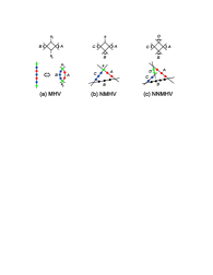
Figure 5: Twistor structure of box integral coefficients for one-loop amplitudes in ${\cal N}=4$ supersymmetric Yang-Mills theory. For each series of amplitudes, (a) MHV ($n_{-}=2$), (b) NMHV ($n_{-}=3$), and (c) NNMHV ($n_{-}=4$), the type of box integral having the simplest nonvanishing coefficient is depicted at the top, and the localization of those coefficients in twistor space is shown at the bottom.

5 What is a twistor string?

I have been remiss in titling this talk “Twistor String Theory and QCD,” without saying anything yet about what twistor string theory is, or how it is related to the more phenomenological developments just outlined. In fact, I won’t describe twistor string theory at any length, but I would like to briefly contrast it with ordinary string theory, from the perspective of methods for computing gauge theory amplitudes.

An ordinary string is an extended object which moves in space-time. Different physical vibrations of the string are associated with different particle states. The higher the harmonic, the more massive the particle; indeed, there is an infinite tower of ultra-heavy particles, as well as a set of massless ones. One of the massless particles is always the graviton. Because the one energy scale in gravity is the Planck mass, $M_{P}\approx 10^{19}$ GeV, this sets the scale for the ultra-heavy masses (unless certain extra dimensions happen to have a large size), as shown in fig. 6(a). Also, the massless spectrum can be relatively complicated — several gauge groups, matter fields transforming in various ways, and so on.

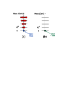
Figure 6: (a) Typical spectrum of particles in ordinary string theory. (b) Typical spectrum in (topological) twistor string theory.

In the early 1990s, this type of string theory was adapted by Bern and Kosower into a tool to compute one-loop QCD amplitudes BernKosower . It worked pretty well. The first computations of the helicity amplitudes for four-gluon scattering in QCD used this technique BernKosower . (The unpolarized cross sections were computed earlier via more traditional methods EllisSexton .) The five-gluon helicity amplitudes were also computed via the string-based method FiveGluon . On the other hand, this string theory was not optimized for QCD calculations. It did not possess all the symmetries of QCD. For example, QCD is classically conformally invariant (independent of energy scale). But traditional string theory depends on the scale $M_{P}$, as reflected in the mass spectrum in fig. 6(a). Related to this fact, a fair amount of analysis was required to decouple the unwanted massive states from the loop amplitudes (as well as the massless states not corresponding to QCD). The analysis would have had to be redone to incorporate external quarks, for example. In the meantime it was found that “abstracting the lessons” from string theory was often the most efficient way to proceed. The efficiency of the string-based rules for amplitudes could be attributed to a background-field quantization of gauge theory BFGauge and a second-order formulation for fermions, for instance BDBFGauge . These lessons could then be applied to amplitudes with external quarks, without having to develop the full string-theoretic machinery QQGGG .

In contrast, the twistor string theory invented by Witten WittenTopologicalString is a topological one, and the string moves in twistor-space, not the usual space-time. “Topological” means that the energy of the string only depends on topological information, so that very few of its degrees of freedom are dynamical. As a result, it does not have a tower of massive states, only massless ones, as shown in fig. 6(b). Twistor string theory is conformally invariant, like classical QCD. It makes much more manifest the symmetries of classical QCD, which include not only conformal invariance, and the secret (${\cal N}=4$) supersymmetry mentioned in section 2, but a full superconformal group containing them. So, from the point of view of calculating QCD amplitudes, twistor string theory seems almost designed to do the job.

On the other hand, twistor string theory is still not precisely QCD. It possesses all the ${\cal N}=4$ superpartners of the gluons, instead of quarks. It also contains gravitons, but not those of Einstein’s theory of gravity; instead they belong to a non-unitary theory, conformal supergravity. Both of these properties are not really an issue for computations of tree-level amplitudes, but they can play havoc with a loop-level description. In fact, there is no satisfactory one-loop formulation of twistor string theory at present. Once again, however, from a computational point of view, abstracting the lessons is often the best.

Even at tree level, such abstraction can be beneficial. Although the MHV $n$-gluon amplitudes (2) could be evaluated directly from the twistor string WittenTopologicalString , and the six-gluon non-MHV amplitudes, such as eq. (14), were also produced in this way RSVI , the MHV rules CSWI have provided a much more efficient method for generic tree amplitudes. They originated at least in part from abstracting the twistor structure which was found by studying existing QCD amplitudes. (One could also say, however, that the MHV rules follow from a different, “disconnected”, prescription for evaluating the relevant twistor-string contributions.)

6 On-shell recursive methods

Another process of abstraction and streamlining led, at the beginning of this year, to the on-shell recursion relations of Britto, Cachazo, Feng and Witten BCFRecursive ; BCFWRecursive . These relations are even more efficient, and lead to more compact formulas, than the MHV rules. Also, they can be proven in a very simple way, using only Cauchy’s theorem and factorization properties. So it is very easy to extend these relations to more general processes, and also to apply the same kinds of techniques to the computation of one-loop amplitudes in QCD.

The path to the on-shell recursion relations was somewhat roundabout, proceeding through the one-loop amplitudes in ${\cal N}=4$ super-Yang-Mills theory, whose box coefficients were sketched in section 4. These amplitudes have infrared divergences, represented in dimensional regularization as poles in $\epsilon=(4-D)/2$. The residues of the poles have to be proportional to the corresponding tree amplitude. This requirement gave new formulas for tree amplitudes, in terms of sums of box coefficients NMHVSeven ; Neq4NMHV ; RSVDissolve , which were more compact than previously-known expressions. Using generalized unitarity, these formulas could be reinterpreted as quadratic recursion relations BCFRecursive

The basic on-shell recursion relation for tree amplitudes reads BCFRecursive ; BCFWRecursive ,

$$A_{n}^{\rm tree}(1,2,\ldots,n)=\sum_{h=\pm 1}\sum_{k=2}^{n-2}A_{k+1}^{\rm tree}(\hat{1},2,\ldots,k,-\hat{K}_{1,k}^{-h}){i\over K_{1,k}^{2}}A_{n-k+1}^{\rm tree}(\hat{K}_{1,k}^{h},k+1,\ldots,n-1,\hat{n}).$$ (15)

It is depicted diagrammatically in fig. 7. The amplitude is represented as a sum of products of lower-point amplitudes, evaluated on shell, but for complex, shifted values of the momenta (see below). The helicity labels of the $n$ external gluons have been omitted, but they are the same on the left- and right-hand sides of eq. (15). For the relation to be valid, the helicities of gluons $n$ and $1$ can be $(h_{n},h_{1})=(-1,1)$, $(1,1)$, or $(-1,-1)$, but not $(1,-1)$. There are two sums. The first is over the helicity $h$ of an intermediate gluon propagating (downward) between the two amplitudes. The second sum is over an integer $k$, which labels the different ways the set $\{1,2,\ldots,n\}$ can be partitioned into two cyclicly-consecutive sets, each containing at least 3 elements, where labels $1$ and $n$ belong to different sets. A hat on top of a momentum label denotes that the corresponding momentum is not that of the original $n$-point amplitude, but is shifted to a different value.

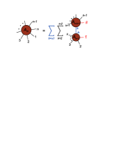
Figure 7: Diagrammatic representation of an on-shell recursion relation for tree amplitudes.

To describe the shifted momenta, first note that, from eq. (4), $k_{i}^{\mu}=\sigma^{\mu}_{\alpha\dot{\alpha}}\lambda_{i}^{\alpha}{\tilde{\lambda}}_{i}^{\dot{\alpha}}$ is a massless four-vector because of the antisymmetry of the spinor products,

$$k_{i}^{2}=\varepsilon_{\beta\alpha}\varepsilon_{\dot{\alpha}\dot{\beta}}({\raise 0.97221pt\hbox to5.52084pt{\hss/\hss}\hbox to0.0pt{\hss$k$}}_{i})^{\alpha\dot{\alpha}}({\raise 0.97221pt\hbox to5.52084pt{\hss/\hss}\hbox to0.0pt{\hss$k$}}_{i})^{\dot{\beta}\beta}=\varepsilon_{\beta\alpha}\lambda_{i}^{\alpha}\lambda_{i}^{\beta}\varepsilon_{\dot{\alpha}\dot{\beta}}{\tilde{\lambda}}_{i}^{\dot{\alpha}}{\tilde{\lambda}}_{i}^{\dot{\beta}}=-\left\langle i\,i\right\rangle\left[i\,i\right]=0\,.$$ (16)

It will continue to be massless even if one of the two spinors is shifted so that it is no longer the complex conjugate of the other spinor, for example

$$\hat{k}_{i}^{\mu}(\sigma_{\mu})_{\alpha\dot{\alpha}}=(\hat{{\raise 0.97221pt\hbox to5.52084pt{\hss/\hss}\hbox to0.0pt{\hss$k$}}}_{i})_{\alpha\dot{\alpha}}=(\hat{\lambda}_{i})_{\alpha}({\tilde{\lambda}}_{i})_{\dot{\alpha}}\,,$$ (17)

where $\hat{\lambda}_{i}$ is shifted away from $\lambda_{i}$.

The momentum shift in the $k^{\rm th}$ term in eq. (15) can now be described as,

$$\lambda_{1} \to \hat{\lambda}_{1}\equiv\lambda_{1}+z_{k}\lambda_{n},\qquad\quad{\tilde{\lambda}}_{1}\to{\tilde{\lambda}}_{1},$$

$$\lambda_{n} \to \lambda_{n},\hskip 85.35826pt{\tilde{\lambda}}_{n}\to\hat{{\tilde{\lambda}}}_{n}\equiv{\tilde{\lambda}}_{n}-z_{k}{\tilde{\lambda}}_{1}\,,$$ (18)

where

$$z_{k}=-{K_{1,k}^{2}\over\langle n^{-}|{\raise 0.91666pt\hbox to9.20833pt{\hss/\hss}\hbox to0.0pt{\hss$K$}}_{1,k}|1^{-}\rangle}\,.$$ (19)

This shift keeps $\hat{{\raise 0.97221pt\hbox to5.52084pt{\hss/\hss}\hbox to0.0pt{\hss$k$}}}_{1}=(\lambda_{1}+z_{k}\lambda_{n}){\tilde{\lambda}}_{1}$ and $\hat{{\raise 0.97221pt\hbox to5.52084pt{\hss/\hss}\hbox to0.0pt{\hss$k$}}}_{n}=\lambda_{n}({\tilde{\lambda}}_{n}-z_{k}{\tilde{\lambda}}_{1})$ massless, as discussed above. It preserves overall momentum conservation, because $\hat{{\raise 0.97221pt\hbox to5.52084pt{\hss/\hss}\hbox to0.0pt{\hss$k$}}}_{1}+\hat{{\raise 0.97221pt\hbox to5.52084pt{\hss/\hss}\hbox to0.0pt{\hss$k$}}}_{n}=\lambda_{1}{\tilde{\lambda}}_{1}+\lambda_{n}{\tilde{\lambda}}_{n}={\raise 0.97221pt\hbox to5.52084pt{\hss/\hss}\hbox to0.0pt{\hss$k$}}_{1}+{\raise 0.97221pt\hbox to5.52084pt{\hss/\hss}\hbox to0.0pt{\hss$k$}}_{n}$. And the intermediate gluon momentum, defined by $\hat{{\raise 0.91666pt\hbox to9.20833pt{\hss/\hss}\hbox to0.0pt{\hss$K$}}}_{1,k}={\raise 0.91666pt\hbox to9.20833pt{\hss/\hss}\hbox to0.0pt{\hss$K$}}_{1,k}+z_{k}\lambda_{n}{\tilde{\lambda}}_{1}$, is also massless (on shell), because

$$\hat{K}_{1,k}^{2}=({\raise 0.91666pt\hbox to9.20833pt{\hss/\hss}\hbox to0.0pt{\hss$K$}}_{1,k}+z_{k}\lambda_{n}{\tilde{\lambda}}_{1})^{2}=K_{1,k}^{2}+z_{k}\langle n^{-}|{\raise 0.91666pt\hbox to9.20833pt{\hss/\hss}\hbox to0.0pt{\hss$K$}}_{1,k}|1^{-}\rangle=0\,.$$ (20)

The derivation of eq. (15) is very simple BCFWRecursive . The momentum shift (18) is considered for an arbitrary complex number $z$, instead of the discrete values $z_{k}$ in eq. (19). This shift defines an analytic function of $z$, $A_{n}^{\rm tree}(z)$. It has poles in $z$ whenever a collection of the shifted momenta, corresponding to an intermediate state, can go on shell. For every allowed partition of $\{1,2,\ldots,n\}$ into $\{1,2,\ldots,k\}\cup\{k+1,\ldots,n-1,n\}$, there is a unique value of $z$ that accomplishes this, $z_{k}$, because $\hat{K}_{1,k}^{2}(z_{k})=0$ according to eq. (20). The desired amplitude is the value of $A_{n}^{\rm tree}(z)$ at $z=0$. Provided that $A_{n}^{\rm tree}(z)\to 0$ as $z\to\infty$, this value at $z=0$ is determined by Cauchy’s theorem in terms of the residues of $A_{n}^{\rm tree}(z)$ at $z=z_{k}$. Using general factorization properties of tree amplitudes, the $k^{\rm th}$ residue evaluates to the product found in the $k^{\rm th}$ term in eq. (15). The vanishing of $A_{n}^{\rm tree}(z)$ as $z\to\infty$ can be established directly from Feynman diagrams for $(h_{n},h_{1})=(-1,1)$ BCFWRecursive . For the other two valid cases it can be shown using the “MHV rules” CSWI , or by a recursive argument BGKS .

No knowledge of twistor space is needed to implement eq. (15). Its derivation is heuristically related to twistor space, however, in that spinors, not vectors, play the fundamental role.

Off-shell recursive approaches to summing Feynman diagrams have a long history BGRecursive ; Mahlon . In the off-shell case, however, the auxiliary lower-point quantities are gauge-dependent. In on-shell recursion relations, in contrast, they are precisely the desired physical, gauge-invariant, on-shell scattering amplitudes, just with fewer partons. In short, trees are recycled into trees.

6.1 A simple application: $A_{6}^{\rm tree}(1^{+},2^{+},3^{+},4^{-},5^{-},6^{-})$

Let us now work through a simple application of eq. (15) BCFRecursive . The first non-MHV $n$-gluon amplitudes (taking into account parity) are those with six gluons, three of positive helicity and three negative. There are three cyclicly-inequivalent helicity configurations: $A_{6}^{\rm tree}(1^{+},2^{+},3^{+},4^{-},5^{-},6^{-})$, $A_{6}^{\rm tree}(1^{+},2^{+},3^{-},4^{+},5^{-},6^{-})$, and $A_{6}^{\rm tree}(1^{+},2^{-},3^{+},4^{-},5^{+},6^{-})$. The last of these amplitudes is related to the first two a “dual Ward identity” (group theory relation) TreeReview . Here we apply eq. (15) to $A_{6}^{\rm tree}(1^{+},2^{+},3^{+},4^{-},5^{-},6^{-})$. Instead of 220 Feynman diagrams (including all color-orderings), there are just three potential on-shell recursive diagrams, shown in fig. 8. Diagrams of the form of fig. 8(a) and fig. 8(c), but with a reversed helicity assignment to the intermediate gluon, vanish because $A_{3}^{\rm tree}(+,+,+)=A_{3}^{\rm tree}(-,-,-)=0$. Figure 8(b), and the corresponding diagram with a reversed intermediate helicity, both vanish using eq. (1). Finally, diagram (c) is related to diagram (a) by the “flip” symmetry $(1\leftrightarrow 6,2\leftrightarrow 5,3\leftrightarrow 4)$ (plus spinor conjugation).

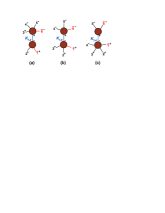
Figure 8: On-shell recursive diagrams for $A_{6}^{\rm tree}(1^{+},2^{+},3^{+},4^{-},5^{-},6^{-})$.

So, remarkably, there is only one independent diagram, fig. 8(a). Its value is given by the product of two shifted MHV amplitudes, each parity-conjugated with respect to eq. (2),

$$D^{(a)} = A_{3}^{\rm tree}(\hat{1}^{+},2^{+},-\hat{K}_{1,2}^{-}){i\over K_{1,2}^{2}}A_{5}^{\rm tree}(\hat{K}_{1,2}^{+},3^{+},4^{-},5^{-},\hat{6}^{-})$$ (21)

$$= {-i\over s_{12}}{{\vphantom{\hat{K}}\left[\smash{\hat{1}}\,\smash{2}\right]}^{3}\over\vphantom{\hat{K}}\left[\smash{2}\,\smash{\hat{K}_{1,2}}\right]\vphantom{\hat{K}}\left[\smash{\hat{K}_{1,2}}\,\smash{\hat{1}}\right]}{{\vphantom{\hat{K}}\left[\smash{\hat{K}_{1,2}}\,\smash{3}\right]}^{3}\over\left[3\,4\right]\left[4\,5\right]\vphantom{\hat{K}}\left[\smash{5}\,\smash{\hat{6}}\right]\vphantom{\hat{K}}\left[\smash{\hat{6}}\,\smash{\hat{K}_{1,2}}\right]}$$

$$= i\,{{\left\langle\smash{6}{\vphantom{1}}^{-}\right|{(1+2)}\left|\smash{3}{\vphantom{1}}^{-}\right\rangle}^{3}\over\left\langle 6\,1\right\rangle\left\langle 1\,2\right\rangle\left[3\,4\right]\left[4\,5\right]s_{612}\left\langle\smash{2}{\vphantom{1}}^{-}\right|{(6+1)}\left|\smash{5}{\vphantom{1}}^{-}\right\rangle}\,.$$

To get the contribution $D^{(c)}$, we add the image of $D^{(a)}$ under the permutation $(1\leftrightarrow 6,2\leftrightarrow 5,3\leftrightarrow 4)$, combined with spinor conjugation, $\langle\ \rangle\,\leftrightarrow[\ ]$. The full amplitude is

$$A_{6}^{\rm tree}(1^{+},2^{+},3^{+},4^{-},5^{-},6^{-}) = i\biggl{[}{{\langle 6^{-}|(1+2)|3^{-}\rangle}^{3}\over\left\langle 6\,1\right\rangle\left\langle 1\,2\right\rangle\left[3\,4\right]\left[4\,5\right]s_{612}\langle 2^{-}|(6+1)|5^{-}\rangle}$$ (22)

$$\hskip 0.0pt+{{\langle 4^{-}|(5+6)|1^{-}\rangle}^{3}\over\left\langle 2\,3\right\rangle\left\langle 3\,4\right\rangle\left[5\,6\right]\left[6\,1\right]s_{561}\langle 2^{-}|(6+1)|5^{-}\rangle}\biggr{]}\,.~{}~{}~{}~{}$$

Let’s compare this representation of the amplitude with the previous one, eq. (14), found using Feynman diagrams. The second expression is shorter. (Here the difference in length is minimal; it becomes more striking for seven gluons BGKSeven ; NMHVSeven .) It also makes manifest the square-root collinear behavior in all channels. For example, in the collinear limit where $k_{3}$ becomes parallel to $k_{4}$, eq. (22) has the correct $1/\left\langle 3\,4\right\rangle$ and $1/\left[3\,4\right]$ behavior manifest; in eq. (14), cancellations between the three terms, each of which behaves like $1/s_{34}$, are required to obtain the proper behavior. On the other hand, eq. (22) contains a spurious singularity, because $\langle 2^{-}|(6+1)|5^{-}\rangle$ vanishes when $k_{6}+k_{1}$ happens to be a linear combination of $k_{2}$ and $k_{5}$ (use the massless Dirac equation to see this). The amplitude is perfectly finite in this region, but each term diverges. In numerically implementing eq. (22), one should take care in this region.

7 One-loop amplitudes

Although the MHV and on-shell recursive rules are quite efficient for the analytical computation of many types of tree amplitudes, and shed a lot of light on their structure, in the end all one really wants are numerical values. Quite efficient numerical computer programs have already been developed over the years, based on off-shell recursive methods RecursivePrograms , which can evaluate QCD tree amplitudes with of order 10 external partons in a reasonable amount of time. In contrast, the complete set of one-loop helicity amplitudes is not known for any pure QCD process with greater than five external legs. There are similar bottlenecks for processes in which a few electroweak vector bosons are produced in addition to multiple QCD partons. So it is of great interest to see whether new methods can be developed for one-loop QCD amplitudes.

The method used to prove the tree-level on-shell recursion relations BCFWRecursive — shifting a pair of momenta by a complex amount, while keeping them on shell — is particularly promising in this regard, because it efficiently incorporates the known factorization of amplitudes onto collinear and multi-particle poles. Indeed, the same techniques can be adopted at one loop, in order to determine the rational (non-logarithmic) parts of amplitudes, once the parts containing branch cuts (logarithms, polylogarithms, etc.) have been determined by other means — for example, using unitarity, as mentioned in section 4. Recently, all the one-loop $n$-gluon helicity amplitudes in QCD with up to two (adjacent) negative-helicity gluons, and an arbitrary number of positive helicity ones, have been produced (or reproduced) in this way BDKLoopFinite ; Bootstrapping . The amplitudes having $n_{-}=0$ or 1 are quite special, because they vanish at tree-level (eq. (1)). They have no infrared or ultraviolet divergences, and there are no branch cuts at all. Also, they were known from previous work BCDK ; Mahlon . They have a purely recursive representation, whose construction involved a few assumptions, which could be cross-checked by comparing to the previous results BDKLoopFinite .

The series of amplitudes $A_{n}^{\rm 1-loop}(1^{-},2^{-},3^{+},4^{+},\ldots,n^{+})$, with two adjacent negative helicities, have branch cuts as well as infrared and ultraviolet divergences. The branch cuts were determined a decade ago, using unitarity Fusing . The rational parts can now be constructed recursively Bootstrapping . In addition to a set of recursive diagrams, much like the tree-level formula (15), there are certain “overlap” diagrams, which perform bookkeeping with respect to certain rational-function terms which naturally accompany the logarithmic terms. There are relatively few diagrams to evaluate. For the rational part of $A_{6}^{\rm 1-loop}(1^{-},2^{-},3^{+},4^{+},5^{+},6^{+})$, for example, there are four nonvanishing recursive diagrams and three nonvanishing overlap diagrams. The evaluation of each diagram is completely algebraic; no loop integrations are required. In contrast, the number of one-loop 6-gluon Feynman diagrams in QCD is 10,680, each of which requires a loop integration.

8 Conclusions

Several new methods for computing gauge theory scattering amplitudes relevant for LHC physics have been developed over the last year or two, with a strong stimulation from twistor string theory. After some abstraction and streamlining, however, many of these methods actually bear a close resemblance to the bootstrap program developed in the 1960s. In a bootstrap, scattering amplitudes are reconstructed directly from their analytic properties, without the need for a Lagrangian Bootstrap ; ELOP . While this program has proven difficult, if not impossible, to carry out in full nonperturbative generality in a strongly-coupled four-dimensional field theory, in the context of perturbation theory much more information is available to assist it. The (factorization) poles of amplitudes are dictated by amplitudes with fewer legs, while the (unitarity) cuts are dictated by products of amplitudes with fewer loops. Tree-level on-shell recursion relations, for example, are a very convenient way of systematically incorporating the factorization data. The use of analyticity fell somewhat out of favor in the the 1970s, with the rise of a Lagrangian (QCD) for the strong interactions. Ironically, it now proves useful to resurrect analyticity, and a perturbative bootstrap, as a tool for computing complicated QCD amplitudes — for which a direct Lagrangian approach, that is, using Feynman rules, can be very cumbersome.

To date, the “practical” spinoffs from twistor-inspired methods have been primarily for tree amplitudes (which can also be obtained by other, numerical methods), and for loop amplitudes in supersymmetric theories. But recently, new one-loop helicity amplitudes in full QCD have begun to fall to these methods, suggesting that soon there will be direct phenomenological applications. In addition, the recent rapid progress in developing new computational approaches along these lines is very likely to continue.

References

- (1) E. Witten, Commun. Math. Phys. 252, 189 (2004) [hep-th/0312171].
-
(2)
D. J. Gross and F. Wilczek,
Phys. Rev. Lett. 30, 1343 (1973);
H. D. Politzer, Phys. Rev. Lett. 30, 1346 (1973). - (3) R. P. Feynman, Phys. Rev. 76 (1949) 769; Phys. Rev. 80, 440 (1950).
-
(4)
M. T. Grisaru, H. N. Pendleton and P. van Nieuwenhuizen,
Phys. Rev. D 15, 996 (1977);
M. T. Grisaru and H. N. Pendleton, Nucl. Phys. B 124, 81 (1977);
S. J. Parke and T. R. Taylor, Phys. Lett. B 157, 81 (1985) [Erratum-ibid. B 174, 465 (1986)];
Z. Kunszt, Nucl. Phys. B 271, 333 (1986). - (5) S. J. Parke and T. R. Taylor, Phys. Rev. Lett. 56, 2459 (1986).
-
(6)
F. A. Berends and W. Giele,
Nucl. Phys. B 294, 700 (1987);
M. L. Mangano, S. J. Parke and Z. Xu, Nucl. Phys. B 298, 653 (1988). -
(7)
M. L. Mangano and S. J. Parke,
Phys. Rept. 200, 301 (1991);
L. J. Dixon, in QCD & Beyond: Proceedings of TASI ’95, ed. D. E. Soper (World Scientific, 1996) [hep-ph/9601359]. - (8) R. Penrose, J. Math. Phys. 8, 345 (1967).
-
(9)
F. A. Berends, R. Kleiss, P. De Causmaecker, R. Gastmans and T. T. Wu,
Phys. Lett. B103, 124 (1981);
P. De Causmaecker, R. Gastmans, W. Troost and T. T. Wu, Nucl. Phys. B206, 53 (1982);
Z. Xu, D. H. Zhang and L. Chang, TUTP-84/3-TSINGHUA;
R. Kleiss and W. J. Stirling, Nucl. Phys. B262, 235 (1985);
J. F. Gunion and Z. Kunszt, Phys. Lett. B161, 333 (1985);
Z. Xu, D. H. Zhang and L. Chang, Nucl. Phys. B291, 392 (1987). - (10) F. A. Berends, W. T. Giele and H. Kuijf, Nucl. Phys. B 333, 120 (1990).
- (11) F. A. Berends and W. T. Giele, Nucl. Phys. B 306, 759 (1988).
- (12) F. Cachazo, P. Svrček and E. Witten, JHEP 0409, 006 (2004) [hep-th/0403047].
- (13) F. Cachazo, P. Svrček and E. Witten, JHEP 0410, 074 (2004) [hep-th/0406177].
-
(14)
G. Georgiou and V. V. Khoze,
JHEP 0405, 070 (2004)
[hep-th/0404072];
J. B. Wu and C. J. Zhu, JHEP 0409, 063 (2004) [hep-th/0406146];
G. Georgiou, E. W. N. Glover and V. V. Khoze, JHEP 0407, 048 (2004) [hep-th/0407027]. -
(15)
L. J. Dixon, E. W. N. Glover and V. V. Khoze,
JHEP 0412, 015 (2004)
[hep-th/0411092];
S. D. Badger, E. W. N. Glover and V. V. Khoze, JHEP 0503, 023 (2005) [hep-th/0412275]. - (16) Z. Bern, D. Forde, D. A. Kosower and P. Mastrolia, Phys. Rev. D 72, 025006 (2005) [hep-ph/0412167].
- (17) C. Schwinn and S. Weinzierl, JHEP 0505, 006 (2005) [hep-th/0503015].
-
(18)
F. Cachazo, P. Svrček and E. Witten,
JHEP 0410, 077 (2004)
[hep-th/0409245];
F. Cachazo, hep-th/0410077;
R. Britto, F. Cachazo and B. Feng, Phys. Rev. D 71, 025012 (2005) [hep-th/0410179]. - (19) Z. Bern, L. J. Dixon, D. C. Dunbar and D. A. Kosower, Nucl. Phys. B 425, 217 (1994) [hep-ph/9403226].
- (20) Z. Bern, V. Del Duca, L. J. Dixon and D. A. Kosower, Phys. Rev. D 71, 045006 (2005) [hep-th/0410224].
- (21) R. Britto, F. Cachazo and B. Feng, Nucl. Phys. B 725, 275 (2005) [hep-th/0412103].
- (22) Z. Bern, L. J. Dixon and D. A. Kosower, Phys. Rev. D72, 045014 (2005) [hep-th/0412210].
-
(23)
L. D. Landau, Nucl. Phys. 13, 181 (1959);
S. Mandelstam, Phys. Rev. 112, 1344 (1958); 115, 1741 (1959);
R. E. Cutkosky, J. Math. Phys. 1, 429 (1960). - (24) Z. Bern, L. J. Dixon and D. A. Kosower, Ann. Rev. Nucl. Part. Sci. 46, 109 (1996) [hep-ph/9602280].
- (25) R. J. Eden, P. V. Landshoff, D. I. Olive and J. C. Polkinghorne, The Analytic Matrix (Cambridge Univ. Press, 1966).
- (26) Z. Bern, L. J. Dixon and D. A. Kosower, Nucl. Phys. B 513, 3 (1998) [hep-ph/9708239].
- (27) R. Britto, F. Cachazo and B. Feng, Phys. Lett. B 611, 167 (2005) [hep-th/0411107].
- (28) A. Brandhuber, B. Spence and G. Travaglini, Nucl. Phys. B 706, 150 (2005) [hep-th/0407214].
-
(29)
S. J. Bidder, N. E. J. Bjerrum-Bohr, L. J. Dixon and D. C. Dunbar,
Phys. Lett. B 606, 189 (2005)
[hep-th/0410296];
S. J. Bidder, N. E. J. Bjerrum-Bohr, D. C. Dunbar and W. B. Perkins, Phys. Lett. B 608, 151 (2005) [hep-th/0412023]; Phys. Lett. B 612, 75 (2005) [hep-th/0502028]. - (30) Z. Bern and D. A. Kosower, Phys. Rev. Lett. 66, 1669 (1991); Nucl. Phys. B 379, 451 (1992).
- (31) R. K. Ellis and J. C. Sexton, Nucl. Phys. B 269, 445 (1986).
- (32) Z. Bern, L. J. Dixon and D. A. Kosower, Phys. Rev. Lett. 70, 2677 (1993) [hep-ph/9302280].
-
(33)
G. ’t Hooft, in Acta Universitatis Wratislavensis no. 38, 12th Winter School of Theoretical Physics in Karpacz, Functional and Probabilistic Methods in Quantum Field Theory,
Vol. 1 (1975);
B. S. DeWitt, in Quantum gravity II, eds. C. Isham, R. Penrose and D. Sciama (Oxford, 1981);
L. F. Abbott, Nucl. Phys. B 185, 189 (1981);
L. F. Abbott, M. T. Grisaru and R. K. Schaefer, Nucl. Phys. B 229, 372 (1983). - (34) Z. Bern and D. C. Dunbar, Nucl. Phys. B 379, 562 (1992).
- (35) Z. Bern, L. J. Dixon and D. A. Kosower, Nucl. Phys. B 437, 259 (1995) [hep-ph/9409393].
- (36) R. Roiban, M. Spradlin and A. Volovich, Phys. Rev. D 70, 026009 (2004) [hep-th/0403190].
- (37) R. Britto, F. Cachazo and B. Feng, Nucl. Phys. B 715, 499 (2005) [hep-th/0412308].
- (38) R. Britto, F. Cachazo, B. Feng and E. Witten, Phys. Rev. Lett. 94, 181602 (2005) [hep-th/0501052].
- (39) R. Roiban, M. Spradlin and A. Volovich, Phys. Rev. Lett. 94, 102002 (2005) [hep-th/0412265].
- (40) S. D. Badger, E. W. N. Glover, V. V. Khoze and P. Svrček, JHEP 0507, 025 (2005) [hep-th/0504159].
- (41) G. Mahlon, Phys. Rev. D 47, 1812 (1993) [hep-ph/9210214]; Phys. Rev. D 49, 2197 (1994) [hep-ph/9311213]; Phys. Rev. D 49, 4438 (1994) [hep-ph/9312276].
-
(42)
F. Caravaglios and M. Moretti,
Phys. Lett. B358, 332 (1995)
[hep-ph/9507237];
F. Caravaglios, M. L. Mangano, M. Moretti and R. Pittau, Nucl. Phys. B539, 215 (1999) [hep-ph/9807570];
P. Draggiotis, R. H. P. Kleiss and C. G. Papadopoulos, Phys. Lett. B439, 157 (1998) [hep-ph/9807207];
A. Kanaki and C. G. Papadopoulos, Comput. Phys. Commun. 132, 306 (2000) [hep-ph/0002082]. - (43) Z. Bern, L. J. Dixon and D. A. Kosower, Phys. Rev. D 71, 105013 (2005) [hep-th/0501240]; hep-ph/0505055.
-
(44)
Z. Bern, L. J. Dixon and D. A. Kosower,
hep-ph/0507005;
D. Forde and D. A. Kosower, hep-ph/0509358. - (45) Z. Bern, G. Chalmers, L. J. Dixon and D. A. Kosower, Phys. Rev. Lett. 72, 2134 (1994) [hep-ph/9312333].
- (46) Z. Bern, L. J. Dixon, D. C. Dunbar and D. A. Kosower, Nucl. Phys. B 435, 59 (1995) [hep-ph/9409265].
- (47) G. F. Chew and S. C. Frautschi, Phys. Rev. Lett. 7, 394 (1961).