Towards the NNLL precision in the decay $\bar{B}\rightarrow X_{s}\gamma$

Abstract:

The present NLL prediction for the decay rate of the rare inclusive process $\bar{B}\rightarrow X_{s}\gamma$ has a large uncertainty due to the charm mass renormalization scheme ambiguity. We estimate that this uncertainty will be reduced by a factor of 2 at the NNLL level. This is a strong motivation for the on-going NNLL calculation, which will thus significantly increase the sensitivity of the observable $\bar{B}\rightarrow X_{s}\gamma$ to possible new degrees of freedom beyond the SM. We also give a brief status report of the NNLL calculation.

PoS(HEP2005)

The inclusive decay $\bar{B}\rightarrow X_{s}\gamma$ is well known as one of the most important flavour observables within the indirect search for new physics [1]. The present experimental accuracy already reached the $10\%$ level, as reflected in the world average of the present measurements [2]:

$$\mbox{BR}[\bar{B}\to X_{s}\gamma]=(3.39^{+0.30}_{-0.27})\times 10^{-4}\,.$$ (1)

In the near future, more precise data on this mode are expected from the $B$-factories. Thus, it is mandatory to reduce the present theoretical uncertainty accordingly. Non-perturbative effects are naturally small within inclusive modes [1]; also additional non-perturbative corrections due to necessary cuts in the photon energy spectrum are under control (see [3]). As was first noticed in [4], there exists a large uncertainty in the theoretical NLL prediction related to the renormalization scheme of the charm-quark mass on which we focus in this article. The reason is that the matrix elements $\langle s\gamma|{O}_{1,2}|b\rangle$, through which the charm-quark mass dependence dominantly enters, vanish at the lowest order (LL) and, as a consequence, the charm-quark mass does not get renormalized in a NLL calculation, which means that the symbol $m_{c}$ can be identified with $m_{c,\rm{pole}}$ or with the $\overline{\mbox{MS}}$ mass $\bar{m}_{c}(\mu_{c})$ at some scale $\mu_{c}$ or with some other definition of $m_{c}$. In a recent theoretical update of the NLL prediction of this branching fraction the ratio $m_{c}/m_{b}$ was varied in the conservative range $0.18\leq m_{c}/m_{b}\leq 0.31$ that covers both the pole mass value (with its numerical error) and the running mass $\bar{m}_{c}(\mu_{c})$ value (with $\mu_{c}\in[m_{c},m_{b}]$), leading to [5]:

$$\mbox{BR}[\bar{B}\to X_{s}\gamma]=(3.70\pm 0.35|_{m_{c}/m_{b}}\pm 0.02|_{\rm{CKM}}\pm 0.25|_{\rm{param.}}\pm 0.15|_{\rm{scale}})\times 10^{-4}\,.$$ (2)

The only way to resolve this scheme ambiguity in a satisfactory way is to perform a systematic NNLL calculation. Working to next-to-next-to-leading-log (NNLL) precision means that one is resumming all the terms of the form

$$(\alpha_{s}(m_{b}))^{p}\,\alpha_{s}^{n}(m_{b})\,\log^{n}(m_{b}/M)\,,\quad(p=0,1,2).$$ (3)

where $M=m_{t}$ or $M=m_{W}$, $n=0,1,2,...\,\,$ . Such a calculation is most suitably done in the framework of an effective low-energy theory. The effective interaction Hamiltonian can be written as

$$H_{\rm{eff}}=-{4G_{F}}/{\sqrt{2}}\,\,\,\,\,\,\,V_{tb}V_{ts}^{*}\,\sum{C_{i}(\mu,M)}\,\,{O}_{i}(\mu)\,,$$ (4)

where ${O}_{i}(\mu)$ are the relevant dimension 6 operators and $C_{i}(\mu,M)$ are the Wilson coefficients.

Parts of the three principal calculational steps leading to the NNLL result within the effective field theory approach are already done: (a) The full SM theory has to be matched with the effective theory at the scale $\mu=\mu_{W}$, where $\mu_{W}$ denotes a scale of order $m_{W}$ or $m_{t}$. The Wilson coefficients $C_{i}(\mu_{W})$ only pick up small QCD corrections, which can be calculated in fixed-order perturbation theory. In the NNLL program, the matching has to be worked out at the order $\alpha_{s}^{2}$. The matching calculation to this precision is already finished, including the most difficult piece, the three-loop matching of the operators ${O}_{7,8}$ [6]. (b) The evolution of these Wilson coefficients from $\mu=\mu_{W}$ down to $\mu=\mu_{b}$ then has to be performed with the help of the renormalization group, where $\mu_{b}$ is of the order of $m_{b}$. As the matrix elements of the operators evaluated at the low scale $\mu_{b}$ are free of large logarithms, the latter are contained in resummed form in the Wilson coefficients. For the NNLL calculation, this RGE step has to be done using the anomalous–dimension matrix up to order $\alpha_{s}^{3}$. While the three-loop mixing among the four-quark operators ${O}_{i}$ $(i=1,\ldots,6)$ [7] and among the dipole operators ${O}_{7,8}$ [8] are already available, the four-loop mixing of the four-quark into the dipole operators is still an open issue. (c) To achieve NNLL precision, the matrix elements $\langle X_{s}\gamma|{O}_{i}(\mu_{b})|b\rangle$ have to be calculated to order $\alpha_{s}^{2}$ precision. This includes also bremsstrahlung corrections. In 2003, the ($\alpha_{s}^{2}\,n_{f}$) corrections to the matrix elements of the operators $O_{1}$,$O_{2}$,$O_{7}$,$O_{8}$ were calculated [9]. Complete order $\alpha_{s}^{2}$ results are available to the $(O_{7},O_{7})$ contribution to the decay width [10]. Recently, also order $\alpha_{s}^{2}$ terms to the photon energy spectrum (away from the endpoint $E_{\gamma}^{\rm{max}}$) were worked out for the operator $O_{7}$ [11].

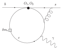
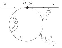
In ref. [12] a strong motivation for this complicated NNLL effort was given by calculating those NNLL terms that are induced by renormalizing the charm-quark mass in the NLL expressions, i.e. those terms that are sensitive to the definition of the charm-quark mass. These terms correspond to $\delta m_{c}$ insertions in the diagrams related to the NLL order matrix elements $M_{1,2}^{\rm{virt}}(m_{c})=\langle s\gamma|{O}_{1,2}(\mu_{b})|b\rangle$ and $M_{1,2}^{\rm{brems}}(m_{c})=\langle s\gamma g|{O}_{1,2}(\mu_{b})|b\rangle$ (for an example, see the left diagram in Fig. 1).

Figure 1: Left: Typical $\delta m_{c}$ insertion diagram. Right: Typical diagram with a self energy insertion.

The sum $\delta M^{\rm{virt}(\epsilon)}_{1,2}(m_{c})\cdot\delta m_{c}$ of all these insertions can be obtained by replacing $m_{c}$ by $m_{c}+\delta m_{c}$ in the $O(\alpha_{s}^{1})$ results $M^{\rm{virt}(\epsilon)}_{1,2}(m_{c})$, followed by expanding in $\delta m_{c}$ up to linear order:

$$M_{1,2}^{\rm{virt}(\epsilon)}(m_{c}+\delta m_{c})=M_{1,2}^{\rm{virt}(\epsilon)}(m_{c})+\delta M^{\rm{virt}(\epsilon)}_{1,2}(m_{c})\cdot\delta m_{c}+O((\delta m_{c})^{2})\,.$$ (5)

As $\delta m_{c}$ is ultraviolet-divergent, the matrix elements $M_{1,2}^{\rm{virt}(\epsilon)}(m_{c})$ are needed in our application up to order $\epsilon^{1}$, as indicated by the notation in eq. (5). In [12] the explicit analytical results for these matrix elements are given in such a way that they can be used in a future complete NNLL calculation. The explicit shift $\delta m_{c}$ depends of course on the renormalization scheme. When aiming at expressing the results for $M_{1,2}^{\rm{virt}(\epsilon)}(m_{c})$ in terms of $\bar{m}_{c}(\mu_{b})$ or $m_{c,\rm{pole}}$, the shift reads ($C_{F}=4/3$)

$$\delta\bar{m}_{c}(\mu_{b})=-\frac{\alpha_{s}(\mu_{b})}{4\pi}\,C_{F}\,\frac{3}{\epsilon}\,\bar{m}_{c}(\mu_{b})\,\,\,\,\mbox{or}\,\,\,\,\delta m_{c,\rm{pole}}=-\frac{\alpha_{s}(\mu_{b})}{4\pi}\,C_{F}\,\left(\frac{3}{\epsilon}+3\ln\frac{\mu_{b}^{2}}{m_{c}^{2}}+4\right)\,m_{c,\rm{pole}}\,.$$

The infinities induced by the $1/\epsilon$ terms in $\delta m_{c}$ get cancelled in a full NNLL calculation, in particular by self-energy diagrams depicted in the right diagram in Fig. 1. When implementing these self-energy insertions, we only took into account the $\Sigma_{1}(p^{2}=m_{c}^{2})$ piece, i.e. that part of the one-loop self-energy which only gets renormalized by the mass parameter. When used at the fixed momentum $p^{2}=m_{c}^{2}$, this piece is gauge-independent.

Our final estimates are given in Fig. 2 for three different values of $\mu_{b}$, where $\mu_{b}$ represents the usual renormalization scale of the effective field theory. Within each vertical string, the solid dot represents the branching ratio using the pole mass $m_{c,\rm{pole}}$, while the open symbols correspond to the $\overline{\mbox{MS}}$ mass $\bar{m}_{c}(\mu_{c})$ for $\mu_{c}=1.25$ GeV (triangle), $\mu_{c}=2.5$ GeV (quadrangle) and $\mu_{c}=5.0$ GeV (pentagon). For each $\mu_{b}$ the left string shows the value of the branching ratio at the NLL level, while the right string shows the corresponding value where, in addition. $\delta m_{c}$ mass insertions and $\Sigma_{1}(p^{2}=m_{c}^{2})$ insertions were taken into account. Because the combination of these insertions is zero by construction for the pole scheme, the solid dots are at the same place in the left and the right string for a given value of $\mu_{b}$. We stress that all the statements made in the following are independent of this absolute normalization introduced by the additional $\Sigma_{1}(p^{2}=m_{c}^{2})$ insertions, because we refer to the reduction of the error only. From Fig. 2 we see that the error related to the charm-quark mass definition is significantly reduced when the NNLL terms connected with mass insertions are taken into account. Taking as an example the results for $\mu_{b}=5$ GeV, we find that at the NLL level the branching ratio evaluated for $\bar{m}_{c}(2.5\ \mbox{GeV})$ is $12.6\%$ higher than the one based on $m_{c,\rm{pole}}$. Including the new contributions, these $12.6\%$ get reduced to $5.1\%$. One also can read off an analogous significant reduction within the $\overline{\mbox{MS}}$ scheme itself. However, to obtain a NNLL prediction for the central value of the branching ratio, it is of course necessary to calculate all NNLL terms.

Figure 2: $\mbox{BR}(b\to X_{s}\gamma)$ for three values of $\mu_{b}$ (see text for more details).