Monte Carlo simulation of the Sivers effect in high-energy proton-proton collisions

Abstract

We present Monte Carlo simulations of the Sivers effect in the polarized Drell-Yan $pp^{\uparrow}\to\mu^{+}\mu^{-}X$ process at the center-of-mass energy $\sqrt{s}=200$ GeV reachable at the Relativistic Heavy-Ion Collider (RHIC) of BNL. We use two different parametrizations for the Sivers function, one deduced from the analysis of Semi-Inclusive Deep-Inelastic Scattering (SIDIS) data at much lower energies, and another one constrained by the RHIC data for the $pp^{\uparrow}\to\pi X$ process at the same energy. For a given luminosity of $10^{32}$ cm^-2 sec^-1, we explore the necessary conditions to reach a statistical accuracy that allows to extract unambiguous information on the structure of the Sivers function. In particular, we consider the feasibility of the test on its predicted universality property of changing sign when switching from SIDIS to Drell-Yan processes.

I Introduction

Azimuthal asymmetries in hard collisions involving (polarized) hadrons represent a formidable testground for Quantum ChromoDynamics (QCD) in the nonperturbative regime. Since almost thirty years, data have been collected for hadron-hadron collisions, and recently also for semi-inclusive $\gamma^{\ast}$-hadron processes in the regime of Deep-Inelastic Scattering (DIS). Large asymmetries were observed in the azimuthal distribution of final-state products (with respect to the normal to the production plane), particularly when flipping the transverse polarization of one hadron involved in the initial or final state: the socalled Single-Spin Asymmetries (SSA). Examples of such SSA are found for the $pp\to\Lambda^{\uparrow}X$ process Bunce et al. (1976) at forward rapidity, for the $pp^{\uparrow}\to\pi X$ process Adams et al. (1991, 2004); Adler et al. (2005); Videbaek (2005) again at forward rapidity, and for the semi-inclusive hadron production $\gamma^{\ast}A^{\uparrow}\to\pi X$, where $A$ is the proton Bravar (2000); Airapetian et al. (2005); Diefenthaler (2005); Avakian et al. (2005) or the deuteron Alexakhin et al. (2005). Apart from the last one, in all other cases SSA up to 40% were detected which were totally unexpected, since they cannot be easily accommodated in a consistent manner within the perturbative QCD in the collinear massless approximation Kane et al. (1978); moreover, they seem to persist also at higher energies typical of the collider regime Adams et al. (2004); Adler et al. (2005); Videbaek (2005), which also contradicts QCD expectations. The same conclusion holds also for unpolarized Drell-Yan experiments at high energy like $\pi A\to\mu^{+}\mu^{-}X$ Falciano et al. (1986); Guanziroli et al. (1988); Conway et al. (1989); Anassontzis et al. (1988), with $A=p,d,W$, and $\bar{p}p\to\mu^{+}\mu^{-}X$ Anassontzis et al. (1988), where the violation of the Lam-Tung sum rule strongly supports the conjecture to go beyond the collinear approximation Conway et al. (1989).

All this amount of puzzling measurements have triggered an intense theoretical activity, particularly about the idea that intrinsic transverse momenta of partons, together with transverse spin degrees of freedom, could be responsible for the observed asymmetries. Transverse-Momentum Dependent (TMD) parton distributions and fragmentation functions have been introduced and linked to measurable asymmetries in the leading-twist cross sections of Semi-Inclusive DIS (SIDIS), Drell-Yan process, semi-inclusive hadron-hadron collision, and $e^{+}e^{-}$ annihilation Ralston and Soper (1979); Collins and Soper (1981, 1982); Collins et al. (1985); Sivers (1990); Collins (1993); Kotzinian (1995); Anselmino et al. (1995); Mulders and Tangerman (1996); Boer and Mulders (1998). As for parton distributions, the prototype of such TMD functions is the Sivers function Sivers (1990), which has a probabilistic interpretation: it describes how the distribution of unpolarized quarks is distorted by the transverse polarization of the parent hadron. Using the notations recommended in Ref. Bacchetta et al. (2004), the Sivers function $f_{1T}^{\perp}$ can be extracted by measuring the socalled Sivers effect in hadron-hadron collisions or SIDIS processes, i.e. an asymmetric distribution of the final-state products in the azimuthal angle defined by the mixed product ${\bm{p}}_{\scriptscriptstyle T}\times{\bm{P}}\cdot{\bm{S}}_{\scriptscriptstyle T}$, where ${\bm{P}}$ is the nucleon momentum and ${\bm{p}}_{\scriptscriptstyle T},{\bm{S}}_{\scriptscriptstyle T}$ are the transverse components of the parton momentum and of the nucleon spin with respect to the direction of ${\bm{P}}$ in the infinite momentum frame. Time-reversal invariance would forbid such correlation if there were no initial/final-state interactions in the considered collision/SIDIS process, respectively. Therefore, $f_{1T}^{\perp}$ is conventionally named a ”naive time-reversal-odd” distribution. The interactions must imply an interference between different helicity states of the target nucleon Brodsky et al. (2002); Ji et al. (2003); consequently, the correlation between ${\bm{p}}_{\scriptscriptstyle T}$ and ${\bm{S}}_{\scriptscriptstyle T}$ is possible only for a nonvanishing orbital angular momentum of the partons. Then, extraction of $f_{1T}^{\perp}$ from data allows to study the orbital motion of hidden confined partons; better, it contains information on their spatial distribution Burkardt and Hwang (2004), and it offers a natural link between microscopic properties of confined elementary constituents and hadronic measurable quantities, such as the nucleon anomalous magnetic moment Burkardt and Schnell (2005).

In QCD, the necessary interactions can be naturally identified with the multiple exchange of soft gluons contained in the gauge link operator, which grants the color gauge-invariant definition of TMD distributions Collins (2002); Ji and Yuan (2002). However, the whole picture relies on the proof of a suitable factorization theorem at small trasverse momenta for the process at hand. At present, QCD factorization proofs have been established for $e^{+}e^{-}$ annihilations Collins and Soper (1981), for Drell-Yan processes Collins et al. (1985), and, more recently, for SIDIS processes Collins and Metz (2004); Ji et al. (2005), including also naive T-odd contributions. The related universality of TMD functions has been carefully discussed in Refs. Collins (2002); Boer et al. (2003); Collins and Metz (2004). It turns out that the Sivers function displays the very interesting property of changing sign when going from the SIDIS to the Drell-Yan process, due to a peculiar feature of its gauge link operator under the time-reversal operation Collins (2002). This interesting prediction has stimulated intense experimental and phenomenological activities to link the Sivers effect recently measured at HERMES Airapetian et al. (2005); Diefenthaler (2005) with processes happening at RHIC, where data are being taken for polarized $pp$ collisions Adler et al. (2005). In particular, three different parametrizations of $f_{1T}^{\perp}$ Anselmino et al. (2005a); Vogelsang and Yuan (2005); Collins et al. (2005a) have been extracted from the HERMES data (and found compatible also with the recent COMPASS data Alexakhin et al. (2005)), and have been used then to make predictions for SSA at RHIC (see also the more recent analysis of Ref. Collins et al. (2005b); for a comparison among the various approaches, see also Ref. Anselmino et al. (2005b)).

In view of the foreseen upgrade of RHIC detector and luminosity (RHIC II), we will consider here the specific Drell-Yan process $pp^{\uparrow}\to\mu^{+}\mu^{-}X$. The leading-twist polarized part of the cross section contains two terms that produce interesting SSA with azimuthal distinct behaviours Boer (1999). In a previous paper Bianconi and Radici (2005a), we analyzed the term weighted by $\sin(\phi+\phi_{S})$, with $\phi$ and $\phi_{S}$ the azimuthal orientations of the final lepton plane and of the proton polarization with respect to the reaction plane; it leads to the extraction of another interesting naive T-odd TMD distribution, the Boer-Mulders $h_{1}^{\perp}$, which is most likely responsible for the above mentioned violation of the Lam-Tung sum rule Boer (1999). In Ref. Bianconi and Radici (2005a), we considered the Drell-Yan process $\bar{p}p^{\uparrow}\to\mu^{+}\mu^{-}X$ at the kinematics of interest for the High Energy Storage Ring (HESR) project at GSI Maggiora et al. (2005); Lenisa et al. (2004) and we numerically simulated the SSA with a Monte Carlo in order to explore the minimal conditions required for an unambiguous extraction of $h_{1}^{\perp}$. Here, we follow the same approach to isolate the other term weighted by $\sin(\phi-\phi_{S})$, which contains the convolution of $f_{1T}^{\perp}$ with the standard unpolarized parton distribution $f_{1}$. The Monte Carlo will be applied to the $pp^{\uparrow}\to\mu^{+}\mu^{-}X$ process at $\sqrt{s}=200$ GeV at the RHIC II luminosity (at least $10^{32}$ cm^-2 sec^-1). The SSA will be numerically simulated using as input both the parametrization of Ref. Anselmino et al. (2005a) and a new high-energy parametrization of $f_{1T}^{\perp}$ constrained by recent RHIC data on SSA for the $pp^{\uparrow}\to\pi X$ process at the same $\sqrt{s}=200$ GeV Adler et al. (2005). The goal is to explore the sensitivity of the simulated asymmetry to different input parametrizations, as well as to directly verify, within the reached statistical accuracy, the predicted sign change of the Sivers function between SIDIS and Drell-Yan Collins (2002).

In Sec. II, the general formalism and details of the numerical simulation are briefly reviewed. In Sec. III, we discuss the input parametrizations. In Sec. IV, results are presented. Finally, in Sec. V some conclusions are drawn.

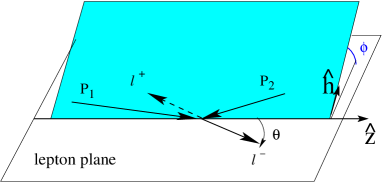
Figure 1: The Collins-Soper frame.

II Theoretical framework and numerical simulations

In a Drell-Yan process, a lepton with momentum $k_{1}$ and an antilepton with momentum $k_{2}$ (with $k_{1(2)}^{2}\sim 0$) are produced from the collision of two hadrons with momentum $P_{1}$, mass $M_{1}$, spin $S_{1}$, and $P_{2},M_{2},S_{2}$, respectively (with $P_{1(2)}^{2}=M_{1(2)}^{2},\;S_{1(2)}^{2}=-1,\;P_{1(2)}\cdot S_{1(2)}=0$). The center-of-mass (cm) square energy available is $s=(P_{1}+P_{2})^{2}$ and the invariant mass of the final lepton pair is given by the time-like momentum transfer $q^{2}\equiv M^{2}=(k_{1}+k_{2})^{2}$. In the kinematical regime where $M^{2},s\rightarrow\infty$, while keeping the ratio $0\leq\tau=M^{2}/s\leq 1$ limited, the lepton pair can be assumed to be produced from the elementary annihilation of a parton and an antiparton with momenta $p_{1}$ and $p_{2}$, respectively. If $P_{1}^{+}$ and $P_{2}^{-}$ are the dominant light-cone components of hadron momenta in this regime, then the partons are approximately collinear with the parent hadrons and carry the light-cone momentum fractions $0\leq x_{1}=p_{1}^{+}/P_{1}^{+},\;x_{2}=p_{2}^{-}/P_{2}^{-}\leq 1$, with $q^{+}=p_{1}^{+},\;q^{-}=p_{2}^{-}$ by momentum conservation Boer (1999). As already anticipated in Sec. I, a key issue is the extraction of TMD parton distributions; this requires the cross section to be kept differential in the transverse momentum of the final lepton pair, ${\bm{q}}_{\scriptscriptstyle T}$, which is bounded by the momentum conservation ${\bm{q}}_{\scriptscriptstyle T}={\bm{p}}_{1{\scriptscriptstyle T}}+{\bm{p}}_{2{\scriptscriptstyle T}}$ to each intrinsic transverse components ${\bm{p}}_{i{\scriptscriptstyle T}}$ of the parton momentum $p_{i}$ with respect to the direction defined by the corresponding hadron momentum ${\bm{P}}_{i}$. If ${\bm{q}}_{\scriptscriptstyle T}\neq 0$ the annihilation direction is not known. Hence, it is convenient to select the socalled Collins-Soper frame Collins and Soper (1977) (see fig. 1), where

$$\hat{t} = \frac{q}{Q}$$

$$\hat{z} = \frac{x_{1}P_{1}}{Q}-\frac{x_{2}P_{2}}{Q}$$

$$\hat{h} = \frac{q_{\scriptscriptstyle T}}{|{\bm{q}}_{\scriptscriptstyle T}|}\;.$$ (1)

The final lepton pair is detected in the solid angle $(\theta,\phi)$, where $\theta$ is defined in Fig. 1 and $\phi$ (and all other azimuthal angles) is measured in a plane perpendicular to $\hat{z},\hat{t}$, but containing $\hat{h}$.

The full expression of the leading-twist differential cross section for the $H_{1}H_{2}^{\uparrow}\to l^{+}l^{-}X$ process can be written as Boer (1999)

$$\frac{d\sigma}{d\Omega dx_{1}dx_{2}d{\bm{q}}_{\scriptscriptstyle T}} = \frac{d\sigma^{o}}{d\Omega dx_{1}dx_{2}d{\bm{q}}_{\scriptscriptstyle T}}+\frac{d\Delta\sigma^{\uparrow}}{d\Omega dx_{1}dx_{2}d{\bm{q}}_{\scriptscriptstyle T}}$$ (2)

$$= \frac{\alpha^{2}}{3Q^{2}}\,\sum_{f}\,e_{f}^{2}\,\Bigg{\{}A(y)\,{\cal F}\left[f_{1}^{f}(H_{1})\,f_{1}^{f}(H_{2})\right]$$

$$\mbox{\hskip 56.9055pt}+B(y)\,\cos 2\phi\,{\cal F}\left[\left(2\hat{\bm{h}}\cdot{\bm{p}}_{1{\scriptscriptstyle T}}\,\hat{\bm{h}}\cdot{\bm{p}}_{2{\scriptscriptstyle T}}-{\bm{p}}_{1{\scriptscriptstyle T}}\cdot{\bm{p}}_{2{\scriptscriptstyle T}}\right)\,\frac{h_{1}^{\perp\,f}(H_{1})\,h_{1}^{\perp\,f}(H_{2})}{M_{1}\,M_{2}}\,\right]\Bigg{\}}$$

$$+\frac{\alpha^{2}}{3Q^{2}}\,|{\bm{S}}_{2{\scriptscriptstyle T}}|\,\sum_{f}\,e_{f}^{2}\,\Bigg{\{}A(y)\,\sin(\phi-\phi_{S_{2}})\,{\cal F}\left[\hat{\bm{h}}\cdot{\bm{p}}_{2{\scriptscriptstyle T}}\,\frac{f_{1}^{f}(H_{1})\,f_{1_{T}}^{\perp\,f}(H_{2})}{M_{2}}\right]$$

$$\mbox{\hskip 85.35826pt}-B(y)\,\sin(\phi+\phi_{S_{2}})\,{\cal F}\left[\hat{\bm{h}}\cdot{\bm{p}}_{1{\scriptscriptstyle T}}\,\frac{h_{1}^{\perp\,f}(H_{1})\,h_{1}^{f}(H_{2})}{M_{1}}\right]$$

$$\mbox{\hskip 85.35826pt}-B(y)\,\sin(3\phi-\phi_{S_{2}})\,{\cal F}\left[\left(4\hat{\bm{h}}\cdot{\bm{p}}_{1{\scriptscriptstyle T}}\,(\hat{\bm{h}}\cdot{\bm{p}}_{2{\scriptscriptstyle T}})^{2}-2\hat{\bm{h}}\cdot{\bm{p}}_{2{\scriptscriptstyle T}}\,{\bm{p}}_{1{\scriptscriptstyle T}}\cdot{\bm{p}}_{2{\scriptscriptstyle T}}-\hat{\bm{h}}\cdot{\bm{p}}_{1{\scriptscriptstyle T}}\,{\bm{p}}_{2{\scriptscriptstyle T}}^{2}\right)\right.$$

$$\mbox{\hskip 199.16928pt}\left.\times\frac{h_{1}^{\perp\,f}(H_{1})\,h_{1T}^{\perp\,f}(H_{2})}{2M_{1}\,M_{2}^{2}}\,\right]\,\Bigg{\}}\;,$$

where $\alpha$ is the fine structure constant, $d\Omega=\sin\theta d\theta d\phi$, $e_{f}$ is the charge of the parton with flavor $f$, $\phi_{S_{i}}$ is the azimuthal angle of the transverse spin of hadron $i$, and

$$A(y)=\left(\frac{1}{2}-y+y^{2}\right)\,\stackrel{{\scriptstyle\mbox{cm}}}{{=}}\,\frac{1}{4}\left(1+\cos^{2}\theta\right) \mbox{\hskip 56.9055pt}B(y)=y(1-y)\,\stackrel{{\scriptstyle\mbox{cm}}}{{=}}\,\frac{1}{4}\,\sin^{2}\theta\;.$$ (3)

The TMD functions $f_{1}^{f}(H),\,h_{1}^{\perp\,f}(H)$, describe the distributions of unpolarized and transversely polarized partons in an unpolarized hadron $H$, respectively, while $f_{1T}^{\perp\,f}(H),\,h_{1T}^{\perp\,f}(H)$, have a similar interpretation but for transversely polarized hadrons $H^{\uparrow}$. The transversity $h_{1}^{f}$ describes transversely polarized partons in transversely polarized hadrons. Each one of these distributions for a parton $f$ is convoluted with its antiparton partner $\bar{f}$ according to

$${\cal F}\left[A^{f}(H_{1})\,A^{f}(H_{2})\right]\equiv\int d{\bm{p}}_{1{\scriptscriptstyle T}}d{\bm{p}}_{2{\scriptscriptstyle T}}\,\delta\left({\bm{p}}_{1{\scriptscriptstyle T}}+{\bm{p}}_{2{\scriptscriptstyle T}}-{\bm{q}}_{\scriptscriptstyle T}\right)\,\left[A(x_{1},{\bm{p}}_{1{\scriptscriptstyle T}};\bar{f}/H_{1})\,A(x_{2},{\bm{p}}_{2{\scriptscriptstyle T}};f/H_{2}^{\uparrow})+(f\leftrightarrow\bar{f})\right]\;.$$ (4)

In previous papers, we analyzed the SSA generated by the azimuthal dependences $\cos 2\phi$ and $\sin(\phi+\phi_{S_{2}})$ in Eq. (2) Bianconi and Radici (2005a), as well as the double-polarized Drell-Yan process Bianconi and Radici (2005b). A combined measurement of these SSA allows to completely determine the unknown transversity $h_{1}$ and Boer-Mulders function $h_{1}^{\perp}$, which could be responsible for the well known violation of the Lam-Tung sum rule Boer (1999) in unpolarized Drell-Yan data Falciano et al. (1986); Guanziroli et al. (1988); Conway et al. (1989) (see also Ref. Boer (2005), and references therein, for a recent discussion on a parallel with QCD vacuum effects). We set up a Monte Carlo simulation of Drell-Yan processes involving unpolarized antiproton beams and transversely polarized protons for various kinematic scenarios at the HESR at GSI, namely for $30<s<200$ GeV² with an antiproton beam energy of 15 GeV and the socalled asymmetric collider mode (proton beams of $~{}3$ GeV) or fixed target mode (proton fixed targets). Special focus was put on the range $4<M<9$ GeV for the lepton invariant mass, since it does not overlap with the charmonium and bottonium resonances (where the elementary annihilation does not necessarily proceed through a simple intermediate virtual photon) and higher-twist corrections should be suppressed justifying the simple approach of Eq. (2) based on the parton model Bianconi and Radici (2005a). Here, we will concentrate on the term weighted by $\sin(\phi-\phi_{S_{2}})$ in Eq. (2) for $H_{1}=p$ and $H_{2}^{\uparrow}=p^{\uparrow}$, and we will consider the related SSA at $\sqrt{s}=200$ GeV reachable at RHIC Bunce et al. (2000). Most of the technical details of the simulation are mutuated from our previous works; hence, we will heavily refer to Refs. Bianconi and Radici (2005a, b) in the following.

The Monte Carlo events have been generated by the following cross section Bianconi and Radici (2005a):

$$\frac{d\sigma}{d\Omega dx_{1}dx_{2}d{\bm{q}}_{\scriptscriptstyle T}}=K\,\frac{1}{s}\,A({\bm{q}}_{\scriptscriptstyle T},x_{1},x_{2},M)\,F(x_{1},x_{2})\,\sum_{i=1}^{4}\,c_{i}({\bm{q}}_{\scriptscriptstyle T},x_{1},x_{2})\,S_{i}(\theta,\phi,\phi_{{}_{S_{2}}})\;.$$ (5)

It means that in Eq. (2) we assume a factorized transverse-momentum dependence in each parton distribution such as to break the convolution ${\cal F}$, leading to the product $A\,F$. The function $A$ is parametrized as Bianconi and Radici (2005a)

$$A(q_{\scriptscriptstyle T},x_{1},x_{2},M)=\frac{5\,\displaystyle{\frac{a}{b}\,\left[\frac{q_{\scriptscriptstyle T}}{b}\right]^{a-1}}}{\left[1+\left(\displaystyle{\frac{q_{\scriptscriptstyle T}}{b}}\right)^{a}\right]^{6}}\;,$$ (6)

where $a(x_{{}_{F}},M),\,b(x_{{}_{F}},M),$ are parametric polynomials given in Appendix A of Ref. Conway et al. (1989) with $x_{{}_{F}}=x_{1}-x_{2}$ and $q_{\scriptscriptstyle T}=|{\bm{q}}_{\scriptscriptstyle T}|$ (see also the more recent Ref. Towell et al. (2001)). It is normalized as

$$\int dq_{\scriptscriptstyle T}\,A(q_{\scriptscriptstyle T},x_{1},x_{2},M)=1\;.$$ (7)

Actually, the Drell-Yan events studied in Ref. Conway et al. (1989) were produced for $\pi-p$ collisions; however, the same analysis, repeated for $\bar{p}-p$ and $p-p$ collisions Anassontzis et al. (1988), gives a similar distribution for $q_{\scriptscriptstyle T}$ not very close to 0 and not much larger than 3 GeV/c. Here, we will adopt two different cuts on $q_{\scriptscriptstyle T}$ depending on the input parametrization for the Sivers function $f_{1T}^{\perp}$ (see next Sec. III), namely $1<q_{\scriptscriptstyle T}<3$ GeV/$c$ and $0.1<q_{\scriptscriptstyle T}<2$ GeV/$c$. Anyway, the average transverse momentum turns out to be $\langle q_{\scriptscriptstyle T}\rangle>1$ GeV/$c$, i.e. much bigger than parton intrinsic transverse momenta induced by confinement.

The latter observation implies that sizeable QCD corrections affect the simple parton model picture of Eq. (2). Their influence on the ${\bm{q}}_{\scriptscriptstyle T}$ distribution is effectively contained in the phenomenological parametrization of Eq. (6). However, there are also other well known corrections Altarelli et al. (1979) coming from the resummation of leading logarithms at any order in the strong coupling constant $\alpha_{s}$, and from the inclusion of diagrams at first order in $\alpha_{s}$ involving the $\bar{q}q$ fusion or the $q\gamma$ Compton mechanisms. The first group, usually named leading-log approximation (LLA), introduces a logarithmic dependence on the scale $M^{2}$ inside the various parameters entering the parton distributions Buras and Gaemers (1978) contained in Eq. (5), such that it would determine their DGLAP evolution. However, the range of $M$ values here explored is close to the one of Refs. Conway et al. (1989); Anassontzis et al. (1988), where the parametrization of $A,F,$ and $c_{i}$ in Eq. (5) was deduced assuming $M$-independent parton distributions. Moreover, as it will be shown in the next Sec. IV, most of the events concentrate around the average $\langle x\rangle\sim 0.1$, where the effects of evolution are almost vanishing. Therefore, similarly to Ref. Bianconi and Radici (2005a, b) we take

$$F(x_{1},x_{2})=\frac{\alpha^{2}}{12Q^{2}}\,\sum_{f}\,e_{f}^{2}\,f_{1}^{f}(x_{1};\bar{f}/H_{1})\,f_{1}^{f}(x_{2};f/H_{2})+(\bar{f}\leftrightarrow f)\;,$$ (8)

which represents the azimuthally symmetric unpolarized part of Eq. (2) that has been factorized out for convenience. As previously stressed, the unpolarized distribution $f_{1}^{f}(x)$ for various flavors $f=u,d,s$, is parametrized as in Ref. Anassontzis et al. (1988).

The second group of QCD corrections is named next-to-leading-log approximation (NLLA), and it is responsible for the well known $K$ factor in Eq. (5). The $K$ factor is roughly independent on $x_{{}_{F}}$ and $M^{2}$ but it can grow with $\sqrt{\tau}$; it also depends on the chosen normalization of the parton distributions (for a detailed analysis in this context see Ref. Anassontzis et al. (1988)). It is a large correction, typically a multiplicative factor in the range $1.5\div 2.5$. Here, we will conventionally assume the same value 2.5 adopted in our previous simulations. But we stress that in an azimuthal asymmetry the corrections to the cross sections in the numerator and in the denominator should compensate each other. This is certainly true for each elementary contribution to the amplitude for SSA, but it is much less obvious for the ratio of full differential cross sections. Indeed, the smooth dependence of the SSA on NLLA corrections has been confirmed for fully polarized Drell-Yan processes at RHIC cm square energies Martin et al. (1998).

The whole solid angle $(\theta,\phi)$ of the final lepton pair in the Collins-Soper frame is randomly distributed in each variable. The explicit form for sorting the angular distribution in the Monte-Carlo is Bianconi and Radici (2005a, b)

$$\sum_{i=1}^{4}\,c_{i}(q_{\scriptscriptstyle T},x_{1},x_{2})\,S_{i}(\theta,\phi,\phi_{S_{2}}) = 1+\cos^{2}\theta+\frac{\nu(x_{1},x_{2},q_{\scriptscriptstyle T})}{2}\,\sin^{2}\theta\,\cos 2\phi$$ (9)

$$+|{\bm{S}}_{2{\scriptscriptstyle T}}|\,c_{4}(q_{\scriptscriptstyle T},x_{1},x_{2})\,S_{4}(\theta,\phi,\phi_{S_{2}})\;.$$

If quarks were massless, the virtual photon would be only transversely polarized and the angular dependence would be described by the functions $c_{1}=S_{1}=1$ and $c_{2}=1,\,S_{2}=\cos^{2}\theta$. Violations of such azimuthal symmetry induced by the function $c_{3}\equiv\textstyle{\frac{\nu}{2}}$ are due to the longitudinal polarization of the virtual photon and to the fact that quarks have an intrinsic transverse momentum distribution, leading to the explicit violation of the socalled Lam-Tung sum rule Conway et al. (1989). QCD corrections influence $\nu$, which in principle depends also on $M^{2}$ (see App. A of Ref. Conway et al. (1989)). Azimuthal $\cos 2\phi$ asymmetries induced by $\nu$ were simulated in Ref. Bianconi and Radici (2005a) using the simple parametrization of Ref. Boer (1999) and testing it against the previous measurement of Ref. Conway et al. (1989).

The last term in Eq. (9) corresponds to the polarized part of the cross section (2). Since we want to single out just the Sivers contribution, we assume that

$$S_{4}(\theta,\phi,\phi_{S_{2}})=(1+\cos^{2}\theta)\,\sin(\phi-\phi_{S_{2}})\;.$$ (10)

Recalling that in Eq. (5) the azimuthally symmetric unpolarized part $A(q_{\scriptscriptstyle T},x_{1},x_{2},M)\,F(x_{1},x_{2})$ of the cross section has been factorized out, the corresponding coefficient $c_{4}$ in Eq. (9) in principle reads

$$c_{4}(q_{\scriptscriptstyle T},x_{1},x_{2})={\bm{S}}_{2{\scriptscriptstyle T}}\,\frac{\sum_{f}\,e_{f}^{2}\,{\cal F}\left[\hat{\bm{h}}\cdot{\bm{p}}_{2{\scriptscriptstyle T}}\,\displaystyle{\frac{f_{1}^{f}(x_{1},{\bm{p}}_{1{\scriptscriptstyle T}})\,f_{1T}^{\perp\,f}(x_{2},{\bm{p}}_{2{\scriptscriptstyle T}})}{M_{2}}}\right]}{\sum_{f}\,e_{f}^{2}\,{\cal F}\left[f_{1}^{f}(x_{1},{\bm{p}}_{1{\scriptscriptstyle T}})\,f_{1}^{f}(x_{2},{\bm{p}}_{2{\scriptscriptstyle T}})\right]}\;,$$ (11)

where the complete dependence of the involved TMD parton distributions has been made explicit. In the next Sec. III, we will discuss two different parametrizations for the $x$ and ${\bm{p}}_{\scriptscriptstyle T}$ dependence of these distributions which allow to calculate the convolutions and determine $c_{4}$.

Following Refs. Bianconi and Radici (2005a, b), the SSA corresponding to the Sivers effect is constructed by dividing the event sample in two groups, one for positive values of $\sin(\phi-\phi_{S_{2}})$ ($U$) and another one for negative values ($D$), and taking the ratio $(U-D)/(U+D)$. Data are accumulated only in the $x_{2}$ bin, i.e. they are summed over in $x_{1},\theta,$ and in $q_{\scriptscriptstyle T}$ with the discussed cutoffs. Contrary to Refs. Bianconi and Radici (2005a, b), no cutoff has been applied to the $\theta$ distribution because $S_{4}$ in Eq. (10) contains the term $1+\cos^{2}\theta$. Statistical errors for $(U-D)/(U+D)$ are obtained by making 10 independent repetitions of the simulation for each individual case, and then calculating for each $x_{2}$ bin the average asymmetry value and the variance. We checked that 10 repetitions are a reasonable threshold to have stable numbers, since the results do not change significantly when increasing the number of repetitions beyond 6. In a real experiment, the SSA would be extracted by taking the ratio between proper differences and sums of cross sections for the four possible combinations with the azimuthal angles $\pm\phi,\,\pm\phi_{S_{2}}$, in order to reduce systematic errors. In the Monte Carlo simulation, for each $\phi_{S_{2}}$ we can simply build the SSA in the $\phi$ angle. In an ideal experiment, the two situations would be equivalent. It is worth noting that while $\phi_{S_{2}}$ is fixed in the lab frame, in the Collins-Soper frame of Fig. 1 it is variable, since the $\hat{h}$ axis is directed along ${\bm{q}}_{\scriptscriptstyle T}/q_{\scriptscriptstyle T}$; hence, a random distribution in $\phi_{S_{2}}$ must be initially extracted in the Monte Carlo.

III Parametrizations of the Sivers function

In our previous papers Bianconi and Radici (2005a, b), the strategy of the numerical simulation was based on making guesses for the input $x$ and ${\bm{p}}_{\scriptscriptstyle T}$ dependence of the parton distributions, and on trying to determine the minimum number of events required to discriminate various SSA produced by very different input guesses. In fact, this would be equivalent to state that in this case some analytic information on the structure of these TMD parton distributions could be extracted from the SSA measurement.

As for the Sivers effect, the situation is different because recently the HERMES collaboration has released new SSA data for the SIDIS process on transversely polarized protons Diefenthaler (2005), which substantially increase the precision of the previous data set Airapetian et al. (2005). As a consequence, three different parametrizations of $f_{1T}^{\perp}$ Anselmino et al. (2005a); Vogelsang and Yuan (2005); Collins et al. (2005a) have been extracted from this data set and found compatible also with the recent COMPASS data Alexakhin et al. (2005). Moreover, a recent preprint appeared which usefully illustrates the differences among the various approaches Anselmino et al. (2005b). At the same time, new data have been collected at RHIC Adler et al. (2005); Videbaek (2005) on SSA in the $pp^{\uparrow}\to\pi X$ process, that confirm the observation of large asymmetries at forward rapidity of the pion also at the high-energy collider regime ($\sqrt{s}=200$ GeV). Despite this class of hadron-hadron collisions is power suppressed and factorization was established in terms of higher-twist correlation operators Qiu and Sterman (1991), still the SSA receives a contribution from the leading-twist convolution $f_{1}\otimes f_{1T}^{\perp}\otimes D_{1}$, where $D_{1}$ describes the fragmentation of an unpolarized quark into the detected $\pi$. Therefore, analogously to the analysis of Ref. D’Alesio and Murgia (2004) at lower energy Adams et al. (1991), we believe that the measured SSA in $pp^{\uparrow}\to\pi X$ processes at $\sqrt{s}=200$ GeV should indirectly constrain the parametrization of $f_{1T}^{\perp}$ and, consequently, the ”strength” of the Sivers effect when these data are ideally interpreted as completely driven by the above convolution.

In our Monte Carlo simulation, we consider two different parametrizations for $f_{1T}^{\perp}$: the one elaborated in Ref. Anselmino et al. (2005a) and based on the new HERMES Diefenthaler (2005) and COMPASS Alexakhin et al. (2005) data, where the ${\bm{p}}_{\scriptscriptstyle T}$ dependence is driven by the $\langle{\bm{p}}_{\scriptscriptstyle T}^{2}\rangle$ extracted in a model dependent way from the azimuthal asymmetry of the unpolarized SIDIS cross section (Cahn effect); a new high-energy parametrization inspired to the one of Ref. Vogelsang and Yuan (2005) but with a specific ${\bm{p}}_{\scriptscriptstyle T}$ dependence constrained by the $pp^{\uparrow}\to\pi X$ data at $\sqrt{s}=200$ GeV.

III.0.1 The parametrization of Ref. Anselmino et al. (2005a)

Keeping in mind the commonly adopted conventions Bacchetta et al. (2004), the expression used in Ref. Anselmino et al. (2005a) is

$$f_{1T}^{\perp\,f}(x,{\bm{p}}_{\scriptscriptstyle T}) = -\frac{M_{2}}{2p_{\scriptscriptstyle T}}\,\Delta^{N}f_{f/p^{\uparrow}}(x,{\bm{p}}_{\scriptscriptstyle T})$$ (12)

$$= -2\,N_{f}\,\frac{(a_{f}+b_{f})^{a_{f}+b_{f}}}{a_{f}^{a_{f}}\,b_{f}^{b_{f}}}\,x^{a_{f}}\,(1-x)^{b_{f}}\,\frac{M_{2}M_{0}}{{\bm{p}}_{\scriptscriptstyle T}^{2}+M_{0}^{2}}\,f_{1}^{f}(x,{\bm{p}}_{\scriptscriptstyle T})$$

$$= -2\,N_{f}\,\frac{1}{\pi\,\langle p_{\scriptscriptstyle T}^{2}\rangle}\,\frac{(a_{f}+b_{f})^{a_{f}+b_{f}}}{a_{f}^{a_{f}}\,b_{f}^{b_{f}}}\,x^{a_{f}}\,(1-x)^{b_{f}}\,\frac{M_{2}M_{0}}{{\bm{p}}_{\scriptscriptstyle T}^{2}+M_{0}^{2}}\,e^{-p_{\scriptscriptstyle T}^{2}/\langle p_{\scriptscriptstyle T}^{2}\rangle}\,f_{1}^{f}(x)\;,$$

where $M_{2}$ is the mass of the polarized proton, $p_{\scriptscriptstyle T}\equiv|{\bm{p}}_{\scriptscriptstyle T}|$, and $\langle p_{\scriptscriptstyle T}^{2}\rangle=0.25$ (GeV/$c$)² is deduced by assuming a Gaussian form for the ${\bm{p}}_{\scriptscriptstyle T}$ dependence of $f_{1}$ in order to reproduce the azimuthal angular dependence of the SIDIS unpolarized cross section (Cahn effect). The parameters $N_{f},a_{f},b_{f},$ with $f=u,d$ are extracted by fitting the recent HERMES Diefenthaler (2005) and COMPASS Alexakhin et al. (2005) data with a final $\chi^{2}$ per degree of freedom of 1.06 (the negligible contribution of antiquarks in the minimization procedure has been traded off for a better precision). They are listed in Tab. 1.

Table 1: Parameters for the Sivers distribution from Ref. Anselmino et al. (2005a)

quark up		quark down
$N_{u}$	$0.32\pm 0.11$	$N_{d}$	$-1.0\pm 0.12$
$a_{u}$	$0.29\pm 0.35$	$a_{d}$	$1.16\pm 0.47$
$b_{u}$	$0.53\pm 3.58$	$b_{d}$	$3.77\pm 2.59$
$M_{0}^{2}$	$0.32\pm 0.25$ (GeV/$c$)2

Following the prediction about a sign change of $f_{1T}^{\perp}$ when going from a SIDIS process (as for the HERMES analysis) to a Drell-Yan process (as it is considered here), we insert the opposite of Eq. (12) inside Eq. (11), including the Gaussian parametrization for $f_{1}(x,{\bm{p}}_{\scriptscriptstyle T})$. The integrals upon the transverse momenta can be evaluated following the steps in Sec.VI of Ref. Boer (1999). The net result is

$$c_{4}\approx|{\bm{S}}_{2{\scriptscriptstyle T}}|\,\frac{4M_{0}\,q_{\scriptscriptstyle T}}{q_{\scriptscriptstyle T}^{2}+4M_{0}^{2}}\,\frac{\sum_{f}\,e_{f}^{2}\,N_{f}\,\displaystyle{\frac{(a_{f}+b_{f})^{a_{f}+b_{f}}}{a_{f}^{a_{f}}\,b_{f}^{b_{f}}}}\,f_{1}(x_{1};\bar{f}/p)\,x_{2}^{a_{f}}\,(1-x_{2})^{b_{f}}\,f_{1}(x_{2};f/p^{\uparrow})}{\sum_{f}\,e_{f}^{2}\,f_{1}(x_{1};\bar{f}/p)\,f_{1}^{f}(x_{2};f/p)+(1\leftrightarrow 2)}\;,$$ (13)

We further simplify this expression by replacing the flavor-dependent product of parton distributions with an average product $\langle f_{1}(x_{1})\rangle\,\langle f_{1}(x_{2})\rangle$ both in the numerator and in the denominator, in order to reduce the statistical noise related to the parametrization of $f_{1}(x)$. The final expression of $c_{4}$ for $pp^{\uparrow}$ collisions, that numerically simulates the Sivers effect in our Monte Carlo, becomes 

$$c_{4}\approx|{\bm{S}}_{2{\scriptscriptstyle T}}|\,\frac{4M_{0}\,q_{\scriptscriptstyle T}}{q_{\scriptscriptstyle T}^{2}+4M_{0}^{2}}\,\frac{1}{9}\,\left[8\,N_{u}\,\frac{(a_{u}+b_{u})^{a_{u}+b_{u}}}{a_{u}^{a_{u}}\,b_{u}^{b_{u}}}\,x_{2}^{a_{u}}\,(1-x_{2})^{b_{u}}\,+\,N_{d}\,\frac{(a_{d}+b_{d})^{a_{d}+b_{d}}}{a_{d}^{a_{d}}\,b_{d}^{b_{d}}}\,x_{2}^{a_{d}}\,(1-x_{2})^{b_{d}}\right]\;.$$ (14)

As it is evident from previous formulae, the parametrization (12) is put in a very convenient form that easily fits the asymmetry term $c_{4}$ in our Monte Carlo. However, the sometimes poor resolution in determining the parameters forced us to select only the central values in Tab. 1 in order to produce meaningful numerical simulations. The sensitivity of the parameters to the HERMES results for the Sivers effect reflects in a more important relative weight of the $d$ quark over the $u$ one in the valence $x$ range, with opposite signs for the corresponding normalization $N_{f},\,f=u,d$. As it will be shown in the next Sec. IV, this has two main consequences on the simulation: small SSA are obtained for the $pp^{\uparrow}\to\mu^{+}\mu^{-}X$ process in the valence $x$ range, where the $\bar{d}d$ annihilation occurs less frequently than the $\bar{u}u$ one; a significant minimum number of events is necessary in the sample to reduce the statistical error bars and make the asymmetry not compatible with zero. From Tab. 1, the $a_{u}$ parameter is much smaller than 1. This means that in Eq. (14) the $u$-quark term dominates at small $x_{2}$, leading to a persistence of the Sivers effect even below the valence $x$ range. This feature is potentially very relevant at RHIC kinematics, where $\langle x\rangle\sim 0.01$. Therefore, for this parametrization we have produced also a specific simulation a small $x_{2}$ with a finer binning $\Delta x_{2}$, as it will be shown in the next Sec. IV. The flavor-independent Lorentzian shape in the ${\bm{p}}_{\scriptscriptstyle T}$ dependence of Eq. (12) produces a maximum asymmetry for $q_{\scriptscriptstyle T}\sim 1$ GeV/$c$ and a rapid decrease for larger values. Consequently, transverse momenta are selected in the range $0.1<q_{\scriptscriptstyle T}<2$ GeV/$c$, because for larger cutoffs the asymmetry is diluted.

III.0.2 A new high-energy parametrization

As already mentioned above, this new parametrization is inspired to the one of Ref. Vogelsang and Yuan (2005). There, it was assumed that the transverse momentum of the detected pion in the SIDIS process was entirely due to the transverse-momentum dependence in the Sivers function. No transverse momenta are contributed by other terms in the factorization formula. In this perspective, this approach can be considered as a limiting case of the approach of Ref. Collins et al. (2005a), based on Gaussian ansätze for the ${\bm{p}}_{\scriptscriptstyle T}$ dependence both in the distribution and fragmentation functions (see Ref. Anselmino et al. (2005b) for a more detailed discussion). In Ref. Vogelsang and Yuan (2005), no further assumption was made but the ${\bm{p}}_{\scriptscriptstyle T}$ distribution was integrated out. As a result, the SSA for the Sivers effect in SIDIS was expressed in terms of ”$\textstyle{\frac{1}{2}}$-moments” of the Sivers function, which were parametrized in terms of the $u$-quark distribution $f_{1}^{u}(x)$ and flavor-dependent normalizations $S_{u},S_{d},$ to be determined by a fit to the new HERMES data Diefenthaler (2005). Also in this case the normalizations turn out to have opposite sign, and the $\chi^{2}$ per degree of freedom is 1.2. The recent COMPASS data Alexakhin et al. (2005) were not included in the fit, but a direct comparison show a qualitative good agreement.

Here, we retain the $x$ dependence of this approach, but we introduce a different flavor-dependent normalization and an explicit ${\bm{p}}_{\scriptscriptstyle T}$ dependence that are bound to the shape of the recent RHIC data on $pp^{\uparrow}\to\pi X$ at $\sqrt{s}=200$ GeV Adler et al. (2005). The expression adopted is

$$f_{1T}^{\perp\,f}(x,{\bm{p}}_{\scriptscriptstyle T}) = N_{f}\,x\,(1-x)\,\frac{M_{2}p_{0}^{2}p_{\scriptscriptstyle T}}{(p_{\scriptscriptstyle T}^{2}+\frac{p_{0}^{2}}{4})^{2}}\,f_{1}^{f}(x,{\bm{p}}_{\scriptscriptstyle T})$$ (15)

$$= N_{f}\,x\,(1-x)\,\frac{M_{2}p_{0}^{2}p_{\scriptscriptstyle T}}{(p_{\scriptscriptstyle T}^{2}+\frac{p_{0}^{2}}{4})^{2}}\,\frac{1}{\pi\,\langle p_{\scriptscriptstyle T}^{2}\rangle}\,e^{-p_{\scriptscriptstyle T}^{2}/\langle p_{\scriptscriptstyle T}^{2}\rangle}\,f_{1}^{f}(x)\;,$$

where $p_{0}=2$ GeV/$c$. Following the same arguments of previous section, we get

$$c_{4}\approx|{\bm{S}}_{2{\scriptscriptstyle T}}|\,x_{2}\,(1-x_{2})\,\left(\frac{2\,p_{0}\,q_{\scriptscriptstyle T}}{q_{\scriptscriptstyle T}^{2}+p_{0}^{2}}\right)^{2}\,\frac{\sum_{f}\,e_{f}^{2}\,N_{f}\,f_{1}(x_{1};\bar{f}/p)\,f_{1}(x_{2};f/p^{\uparrow})}{\sum_{f}\,e_{f}^{2}\,f_{1}(x_{1};\bar{f}/p)\,f_{1}^{f}(x_{2};f/p)+(1\leftrightarrow 2)}\;.$$ (16)

Again, we can further simplify the expression introducing the flavor average product $\langle f_{1}(x_{1})\rangle\,\langle f_{1}(x_{2})\rangle$, which leads to 

$$c_{4}\approx|{\bm{S}}_{2{\scriptscriptstyle T}}|\,x_{2}\,(1-x_{2})\,\left(\frac{2\,p_{0}\,q_{\scriptscriptstyle T}}{q_{\scriptscriptstyle T}^{2}+p_{0}^{2}}\right)^{2}\,\frac{8\,N_{u}+N_{d}}{9}\;.$$ (17)

The $q_{\scriptscriptstyle T}$ shape is different from Eq. (14) and the peak position is shifted at much larger values. This is in agreement with a similar analysis of the azimuthal asymmetry of the unpolarized Drell-Yan data (the violation of the Lam-Tung sum rule Boer (1999)). But, more specifically, it is induced by the observed $x_{{}_{F}}-q_{\scriptscriptstyle T}$ correlation in the RHIC data for $pp^{\uparrow}\to\pi X$, when it is assumed that the SSA is entirely due to the Sivers mechanism; this suggests that the maximum asymmetry is reached in the upper valence region such that $x_{{}_{F}}\approx x_{2}\sim\langle q_{\scriptscriptstyle T}\rangle/5$ Adler et al. (2005). We have conveniently modified the cutoffs such that for this parametrization the sampled distribution is $1<q_{\scriptscriptstyle T}<3$ GeV/$c$. In this case, the peak asymmetry is reached for $x_{2}\sim 0.5$ (see next Sec. IV). Contrary to the other Lorentzian and Gaussian distributions adopted so far, the ${\bm{p}}_{\scriptscriptstyle T}$ distribution of Eq. (15) cannot be normalized in the usual way because of lack of convergence at large $q_{\scriptscriptstyle T}$. Rather, it is built as to assume the value 1 on its peak position $q_{\scriptscriptstyle T}=p_{0}$. Finally, the flavor dependence of the normalization is kept as simple as in Ref. Collins et al. (2005a), namely $N_{u}=-N_{d}=0.7$. The sign, positive for $u$ quark and negative for the $d$, already takes into account the predicted sign change of $f_{1T}^{\perp}$ from Drell-Yan to SIDIS, where the opposite flavor dependence of the sign was obtained Anselmino et al. (2005a); Vogelsang and Yuan (2005); Collins et al. (2005a).

IV Results of the Monte Carlo simulations

In this Section, we present results for Monte Carlo simulations of the Sivers effect in the Drell-Yan process $pp^{\uparrow}\to\mu^{+}\mu^{-}X$ using input from the previous Sec. III.0.1 and III.0.2. The goal is to explore the sensitivity of the simulated asymmetry to different input parametrizations (i.e. to the input theoretical uncertainty), as well as to directly verify, within the reached statistical accuracy, the predicted sign change of the Sivers function between SIDIS and Drell-Yan Collins (2002). The collision is considered at the cm energy $\sqrt{s}=200$ GeV, at which RHIC is presently taking data. We use a conservative dilution factor 0.5 for the proton polarization, even if a foreseen upgrade of the superconducting siberian snake will allow RHIC to run in the future with stable 70% transverse polarization Aidala (2005). We select two different ranges for the lepton invariant mass: $4<M<9$ GeV and $12<M<40$ GeV. In this way, we avoid overlaps with the resonance regions of the $\bar{c}c$ and $\bar{b}b$ quarkonium systems. At the same time, the theoretical analysis based on the leading-twist cross section (2) should be well established, since higher-twist effects can be classified according to powers of $M_{p}/M$, where $M_{p}$ is the proton mass. Moreover, at $\sqrt{s}=200$ GeV also the QCD corrections beyond tree level should be suppressed, which justifies the approximations described in Sec. II. In the Monte Carlo, the events are sorted according to the cross section (5), supplemented by Eqs. (6)-(8), while the asymmetry related to the Sivers effect is simulated by Eqs. (9), (10), (14) and (17). In particular, the events are divided in two groups, one for positive values ($U$) of $\sin(\phi-\phi_{S_{2}})$ in Eq. (10), and another one for negative values ($D$), and taking the ratio $(U-D)/(U+D)$. Data are accumulated only in the $x_{2}$ bins of the polarized proton, i.e. they are summed over in the $x_{1}$ bins for the unpolarized proton, in the transverse momentum $q_{\scriptscriptstyle T}$ of the muon pair and in their zenithal orientation $\theta$. Proper cuts are applied to the $q_{\scriptscriptstyle T}$ distribution according to the different input parametrization of the Sivers function: for the case of Sec. III.0.1, $0.1<q_{\scriptscriptstyle T}<2$ GeV/$c$; for the case of Sec. III.0.2, $1<q_{\scriptscriptstyle T}<3$ GeV/$c$. In this way, the ratio between the absolute sizes of the asymmetry and the statistical errors is optimized for each choice. The resulting $\langle q_{\scriptscriptstyle T}\rangle$ is $\sim 1.8$ GeV/$c$, in fair agreement with the one experimentally explored at RHIC Adler et al. (2005). Contrary to Refs. Bianconi and Radici (2005a, b), there is no need to introduce cuts in the $\theta$ distribution because of the $(1+\cos^{2}\theta)$ term in Eq. (10). We have considered two initial different samples of $20\,000$ and $100\,000$ events. Statistical errors for $(U-D)/(U+D)$ are obtained by making 10 independent repetitions of the simulation for each individual case, and then calculating for each $x_{2}$ bin the average asymmetry value and the variance. We checked that 10 repetitions are a reasonable threshold to have stable numbers, since the results do not change significantly when increasing the number of repetitions beyond 6.

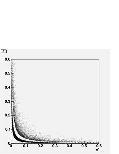
Figure 2: The scatter plot for $120\,000$ events of Drell-Yan muon pairs produced by proton-proton collisions at $\sqrt{s}=200$ GeV. The two bands in which data are grouped, correspond to two different ranges in the muon invariant mass: $4<M<9$ GeV for the lower band, $12<M<40$ GeV for the upper one.

IV.1 Properties of the phase space

In Fig. 2, the scatter plot (in the fractional momenta $x_{1}\equiv x^{\prime},x_{2}\equiv x,$ of the annihilating partons) for $120\,000$ events of Drell-Yan muon pairs produced by proton-proton collisions at $\sqrt{s}=200$ GeV, is shown. The data are divided in two different bands, corresponding to two different ranges in the muon pair invariant mass: $4<M<9$ GeV for the lower band and $12<M<40$ GeV for the upper one. In fact, hyperboles $x_{1}x_{2}=const.$ are selected by fixed values of $\tau=x_{1}x_{2}=M^{2}/s$. Since the elementary annihilation is assumed to proceed through a virtual photon, the cross section contains a term $1/M^{2}\sim 1/\tau$ which populates the phase space at low values, while the upper right corner of Fig. 2 for $\tau\to 1$ is basically empty (also because the parton distributions vanish for $x_{1/2}\to 1$). Therefore, within each band events tend to accumulate to the lowest possible $M$ in the considered range, which means that they try to align along the hyperbole with lowest possible values of $x_{1}$ and $x_{2}$. Moreover, for the same reason the lower band is much more dense than the other one: 95% of the events correspond to the $4<M<9$ GeV range. This is why we consider also this case, because the much higher statistics can be traded for the questionable neglect of higher-twist contributions with respect to the higher $12<M<40$ GeV range.

The scatter plot of Fig. 2 contains two main differences with respect to our previous analysis of Ref. Bianconi and Radici (2005a) for the GSI setup, where the $\bar{p}p^{\uparrow}\to\mu^{+}\mu^{-}X$ process was considered at $\sqrt{s}=14$ GeV. First of all, here the cm energy is higher by one order of magnitude, which means that $x_{1/2}$ values lower by one order of magnitude are explored, typically $\langle x_{1/2}\rangle\sim 0.01$. Secondly, this is emphasized by the fact that in $pp$ collisions at least one of the two annihilating partons comes from the proton sea distribution, which is peaked at very low $x$ values. The importance of parton momenta below the valence region is potentially relevant to the theoretical models. We already mentioned in Sec. III.0.1 that the parametrization of Eq. (12) leads to a persistence of the Sivers effect in this range, contrary to the other one of Eq. (15). Anyway, both choices lead to a vanishing effect for $x_{2}\to 0$. The dominance of the low $x_{2}$ portion of phase space is evident in the histograms for the event distributions displayed in the next Sec. IV, where the first bin $[0,0.1]$ contains more than 50% of events on average. We can also estimate the expected position of the peak density, assuming that the bidimensional event distribution $N(x_{1},x_{2})$ is dominated by the $1/\tau$ factor associated to the elementary $\bar{q}q$ fusion into a virtual photon. In this case, $N(x_{1},x_{2})=1/(x_{1}x_{2})$ for $\tau>M^{2}_{min}/s$, and 0 otherwise. Consequently, the $x_{1}$-integrated distribution has the form $\log(x_{2}s/M^{2}_{min})/x_{2}$ and reaches its peak value for $\log(x_{2}s/M^{2}_{min})=1$, i.e. for $x_{2}=eM^{2}_{min}/s\approx 3M^{2}_{min}/s\sim 0.01$ for $\sqrt{s}=200$ GeV and $M_{min}=12$ GeV, in agreement with the average values produced by the Monte Carlo. Elsewhere, the integrated distribution behaves like $1/x_{2}$, as it can visually be checked in the histograms of next Sec. IV.

The $1/\tau$ mechanism in the random generation can artificially suppress the asymmetry irrespective of the size of the Sivers function itself. In fact, let us consider the $12<M<40$ GeV range, which has a lower event rate; we distinguish four different slices of phase space:

• $x_{1},x_{2}>0.1$ : this part covers 99% of the phase space, but it contains only 0.5% of the total number of events; it corresponds to higher $M$ values ($M>20$ GeV) and it is suppressed by the $1/M^{2}$ mechanism; moreover, in $F(x_{1},x_{2})$ of Eq. (8) the annihilating antiquark with flavor $\bar{f}$ is picked up from the sea distribution of one of the two protons at large $x$;

• $x_{1},x_{2}<0.1$ : this part covers $<1$% of the phase space, but it contains 20% of events; in fact, it corresponds to lower $M$ values (emphasized by the $1/M^{2}$ mechanism) and $F(x_{1},x_{2})$ is dominated by the sea distributions in both protons, that are enhanced at small $x$; however, the SSA is suppressed because $f_{1T}^{\perp}/f_{1}\to 0$ for $x_{2}\to 0$;

• $x_{1}>0.1,x_{2}<0.1$ : this part covers again $<1$% of the phase space, but it contains 40% of the events; it is less favoured by the $1/M^{2}$ mechanism with respect to the previous case, but $F(x_{1},x_{2})$ contains the term $f_{1}(x_{1};f/p)\,f_{1}(x_{2};\bar{f}/p)$, that is dominant in this slice of phase space; however, for the very same reason the SSA is suppressed because it is approximately driven by $f_{1T}^{\perp}(x_{2})/f_{1}(x_{2};\bar{f}/p)\to 0$ for $x_{2}\to 0$;

• $x_{1}<0.1,x_{2}>0.1$ : all previous arguments apply also here upon the $x_{1}\leftrightarrow x_{2}$ exchange but for the SSA, which is driven by $f_{1T}^{\perp}(x_{2})/f_{1}(x_{2};f/p)$ and, therefore, it is not suppressed for $x_{2}>0.1$.

In summary, irrespective of the size of the Sivers function, the magnitude of the corresponding SSA is suppressed in all parts of phase space but in the region $x_{1}<0.1,x_{2}>0.1$, dominated by the sea partons of the unpolarized proton and by the valence partons of the polarized one. Elsewhere, the $1/M^{2}$ mechanism induces a dominance of the sea partons, that acts as an effective dilution factor leading to a waste of $\sim 50$% of the total number of events.

IV.2 Total cross section and event rates

Using Eq. (8) with the parametrization for the parton distributions from Ref. Conway et al. (1989), from our Monte Carlo we deduce a total cross section $\sigma_{pp}=0.1$ nb for the $pp\to\mu^{+}\mu^{-}X$ process at $\sqrt{s}=200$ GeV and with invariant masses in the range $12<M<40$ GeV, while we get $\sigma_{pp}=1.2$ nb for the lower $4<M<9$ GeV range. The results are quite sensitive to the parametrization of the parton distributions. We have recalculated the total cross sections with the more recent NNLO analysis of Ref. Martin et al. (2002) and we get 0.4 nb and 7 nb, respectively. When changing parametrizations and, consequently, normalizations, we had to readjust the $K$ factor accordingly; in order to reproduce the measured cross section at $\sqrt{s}\approx 16$ GeV Conway et al. (1989), we had to reduce it by 50%. It means that now $K\approx 1$ and the QCD corrections are mostly contained in the NNLO parametrization of the parton distributions. The sensitivity (and the related uncertainty) of this analysis to the input are sizeable, but do not alter the order of magnitude of the result. Since our goal is to estimate event rates by multiplying $\sigma_{pp}$ with a given luminosity, we are confident that the results are realistic and reliable. For RHIC, a luminosity of $10^{32}$ cm^-2 sec^-1 or higher is foreseen Bunce et al. (2000). This means, for example, that at least $250\,000$ Drell-Yan events/month (and up to 7 times more) could be collected with this luminosity and muon pair invariant masses in the $4<M<9$ GeV range. A list of the combinations here explored is given in Tab. 2 (for a more comprehensive analysis see Ref. Bianconi (2005)).

Table 2: Total cross sections for Drell-Yan $pp$ collisions at $\sqrt{s}=200$ GeV and for various invariant masses of the muon pair, at the given luminosity $10^{32}$ cm^-2 sec^-1.

$f_{1}(x)$ from	$M$ (GeV)	$\sigma_{pp}$ (nb)	rates (events/month)
Ref. Conway et al. (1989)	$4\div 9$	1.2	$2.5\times 10^{5}$
Ref. Conway et al. (1989)	$12\div 40$	0.1	$2.5\times 10^{4}$
Ref. Martin et al. (2002)	$4\div 9$	7	$1.5\times 10^{6}$
Ref. Martin et al. (2002)	$12\div 40$	0.4	$10^{5}$

It is also interesting to compare with the antiproton-proton Drell-Yan collision. In general, we expect that the lower the $\langle x\rangle$, the more the cross sections are dominated by sea parton distributions, the closer the ratio $\sigma_{\bar{p}p}/\sigma_{pp}$ approaches 1. By updating our previous results Bianconi and Radici (2005a) at the present energy and viceversa, we get

$$\frac{\sigma_{\bar{p}p}}{\sigma_{pp}}(\sqrt{s}=200;4<M<9)=2 \mbox{\hskip 28.45274pt}\frac{\sigma_{\bar{p}p}}{\sigma_{pp}}(\sqrt{s}=200;12<M<40)=4 \frac{\sigma_{\bar{p}p}}{\sigma_{pp}}(\sqrt{s}=14;4<M<9)=40\;.$$ (18)

There are two ways to lower the range of $x$ or, equivalently, $\tau$: decreasing the invariant mass $M$, or increasing the cm energy $\sqrt{s}$. Indeed, the results show that for this trend the ratio approaches 1. When increasing $\sqrt{s}$ at a given $M$ range, for example, the depletion of the ratio implies also that $\sigma_{pp}$ increases. This curious result of an increasing cross section with energy can be explained by recalling that a shift to smaller $x_{1},x_{2},$ makes $F(x_{1},x_{2})$ in Eq. (8) dominated by the sea parton distributions, which are large at very small parton momenta.

Figure 3: The sample of $20\,000$ Drell-Yan events for the $pp^{\uparrow}\to\mu^{+}\mu^{-}X$ reaction at $\sqrt{s}=200$ GeV, $12<M<40$ GeV, and $1<q_{\scriptscriptstyle T}<3$ GeV/$c$, using the parametrization of Eq. (15) (see text). Upper panel: for each bin in the parton momentum $x_{2}$ inside $p^{\uparrow}$, the darker histogram collects events with positive $\sin(\phi-\phi_{S_{2}})$ $(U)$, the superimposed lighter histogram collects the negative ones $(D)$. Lower panel: the asymmetry $(U-D)/(U+D)$; upward triangles for $N_{u}>0$ in Eq. (15) corresponds to a sign change in the Sivers function from SIDIS to Drell-Yan processes; squares for $N_{u}<0$. Statistical error bars from 10 independent repetitions of the simulation. Continuous lines are drawn to guide the eye.

IV.3 Single-spin asymmetries

In Fig. 3, the sample of $20\,000$ Drell-Yan events for the $pp^{\uparrow}\to\mu^{+}\mu^{-}X$ reaction at $\sqrt{s}=200$ GeV is displayed for muon invariant mass in the $12<M<40$ GeV range. Results are reported in $x_{2}$ bins excluding the upper boundary $x_{2}>0.8$, which is scarcely or not at all populated, according to the upper band in Fig. 2. Events are accumulated according to Eq. (17) based on the parametrization (15) of the Sivers function; consequently, the transverse momentum distribution is constrained by $1<q_{\scriptscriptstyle T}<3$ GeV/$c$. In the upper panel, for each bin two groups of events are stored, one corresponding to positive values of $\sin(\phi-\phi_{S_{2}})$ in Eq. (10) (represented by the darker histogram), and one for negative values (superimposed lighter histogram). In the lower panel, the asymmetry $(U-D)/(U+D)$ is shown between the positive $(U)$ and negative $(D)$ values. Average values of the asymmetry and (statistical) error bars are obtained by 10 independent repetitions of the simulation. The upward triangles indicate the results assuming a positive normalization for the quark $u$ in Eq. (15), which already takes into account the predicted sign change of $f_{1T}^{\perp}$ from Drell-Yan to SIDIS Collins (2002) with respect to recent parametrizations of SIDIS data Anselmino et al. (2005a); Vogelsang and Yuan (2005); Collins et al. (2005a). For sake of comparison, the squares illustrate the opposite results that one would obtain ignoring such prediction.

From the upper panel of Fig. 3, we deduce that the assumed elementary $\bar{q}q\to\gamma^{\ast}$ mechanism indeed populates the phase space for the lowest possible $\tau$, with more than 50% of the events in the $0<x_{2}<0.1$ bin, leaving a $\sim 1/x_{2}$ distribution outside. In the lower panel, correspondingly, the error bars are small for $x_{2}<0.5$ and allow for a clean reconstruction of the asymmetry shape and, more importantly, for a conclusive test of the predicted sign change in $f_{1T}^{\perp}$. With the considered sample of $20\,000$ events, the same conclusion is not possible using the parametrization of Eq. (12), because the asymmetry produced by Eq. (14) is too small. More quantitatively, half of the displayed error bar representes the variance $\Delta A(x_{2})$ for the asymmetry $A=(U-D)/(U+D)$ in each $x_{2}$ bin. The results in the lower panel of Fig. 3 can be approximated by the relation $\Delta A\approx 0.05\,x_{2}$. The asymmetry is statistically not compatible with zero if $A(x_{2})>\Delta A=0.05\,x_{2}$ for the considered $x_{2}$ range. With $20\,000$ events, this condition is fulfilled only by the parametrization (15), but not by the one in Eq. (12). Finally, from Tab. 2 we deduce that an hypothetical experiment in these kinematic conditions should run from one week to, at most, almost one month in order to reach the indicated statistical error bars.

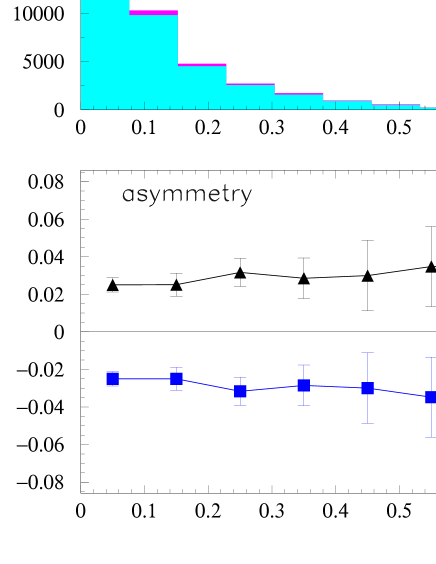
Figure 4: Same as in Fig. 3 but considering $100\,000$ events using the parametrization of Eq. (12) and $0.1<q_{\scriptscriptstyle T}<2$ GeV/$c$ (see text). Lower panel: upward triangles for $N_{u}>0$ in Eq. (14), squares for $N_{u}<0$.

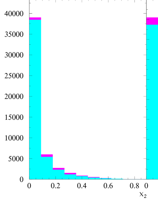
Figure 5: The sample of $100\,000$ Drell-Yan events for the same reaction in the same conditions and notations as in Fig. 3 but for $4<M<9$ GeV. Left panel: parametrization of Eq. (15); right panel: parametrization of Eq. (12) (see text).

In Fig. 4, we consider the same kinematic conditions of the previous Fig. 3 but with a sample of $100\,000$ events, which would require at least one month of running time, or four months in the most disfavoured conditions. We employ the parametrization of Eq. (12). We recall that the $q_{\scriptscriptstyle T}$ distribution is now integrated in the range $0.1<q_{\scriptscriptstyle T}<2$ GeV/$c$ with a resulting lower $\langle q_{\scriptscriptstyle T}^{2}\rangle$ (see previous Sec. III.0.1). Notations in the figure are the same as in the previous Fig. 3. In particular, in the lower panel upward triangles identify the results from Eq. (14) with $N_{u}>0$ from Tab. 1; squared points refer to the opposite choice. Therefore, we conclude that the parametrization (12) demands for a much higher statistics in order to get a clear nonvanishing shape, because it produces an overall smaller asymmetry. Still, a definite answer is possible about the sign change prediction of $f_{1T}^{\perp}$ if the statistical sample meets the required conditions.

In Fig. 5, we show just the histogram of collected $100\,000$ events in the same conditions and notations as before but for the lower $4<M<9$ GeV range. From Tab. 2, we note that the necessary running time is $2\div 3$ times shorter than the one for collecting $20\,000$ events at the higher $12<M<40$ GeV range, depending on the parametrization chosen for $f_{1}$. Again, this is due to the already mentioned $1/\tau$ factor of the elementary $\bar{q}q\to\gamma^{\ast}$ mechanism, which privileges lower $\tau$. For the very same reason, an even larger portion of events (77%) is contained in the first $0<x_{2}<0.1$ bin, while the remaining 23% is distributed for $x_{2}>0.1$ approximately as $1/x_{2}$.

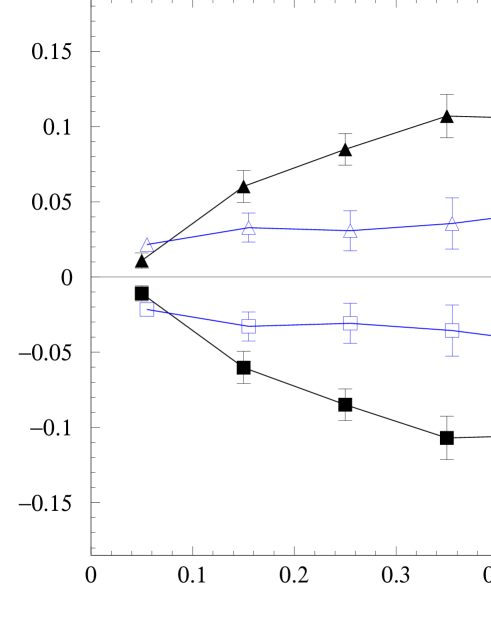
Figure 6: The asymmetry $(U-D)/(U+D)$ corresponding to the histograms of Fig. 5, where $U$ identifies the darker histograms and $D$ the superimposed lighter ones (see text). Upward triangles for the parametrization of Eq. (15) with $N_{u}>0$; squares for $N_{u}<0$. Open upward triangles for the parametrization of Eq. (12) with $N_{u}>0$; open squares for $N_{u}<0$.

In Fig. 6, we plot the spin asymmetries corresponding to the histograms of the previous Fig. 5. Notations are the following. Upward triangles correspond to the histograms in the left panel of Fig. 5, i.e. to the parametrization of Eq. (15); the flavor dependent normalization is $N_{u}>0$, according to the properties of $f_{1T}^{\perp}$ as it is extracted from SIDIS data. The corresponding choice $N_{u}<0$ is represented by the squares. The open upward triangles and squares show the results for the other parametrization Eq. (12). The accumulation of events for very low $x_{2}$ values, which is evident in Fig. 5, here reflects in very tiny error bars for the same bins, allowing to clearly distinguish the two different parametrizations for $0<x_{2}\lesssim 0.5$. In this range, a measurement of the Sivers effect for invariant masses as low as $4<M<9$ GeV, allows to reduce the theoretical uncertainties in very few days of running time (from 2 to 12, depending on the parametrization of the unpolarized parton distributions). Moreover, and most important, in the same $x_{2}$ range the statistical accuracy is sufficient to directly test the predicted sign change of $f_{1T}^{\perp}$ Collins (2002), irrespective of the uncertainty in the theoretical input.

For $0.5\lesssim x_{2}$, the width of the error bars does not always allow for such analysis, since the variance grows approximately as $\Delta A\approx 0.04\,x_{2}$. We already noted that for $12<M<40$ GeV approximately half of the $20\,000$ events lie in the valence range $0.1<x_{2}<0.7$ (see the upper panel in Fig. 3), while for $4<M<9$ GeV $23\,000$ events out of $100\,000$ are found in the same range (see Fig. 5). If we assume that the size of the error bars is proportional to $1/\sqrt{N}$, with $N$ the number of events, then, in the valence region for a given parametrization, the size of the error bars for the higher $M$ range should approximately scale as $\sqrt{23/10}\approx 1.5$ with respect to the one for the lower $M$ range. It is easy to check from the upward triangles in Fig. 3 and Fig. 6 that for the parametrization (15) indeed this approximate relation is verified. But from Tab. 2, we deduce also that in the same running time necessary to collect $20\,000$ events at $12<M<40$ GeV it is possible to collect $200\,000\div 300\,000$ events at $4<M<9$ GeV, depending on the chosen parametrization. In the valence range, this means $46\,000\div 70\,000$ events (the 23% of the total, as before), which induces a reduction factor $2\div 2.5$ in the size of the error bars. Therefore, we can put a sort of ”normalization” for the approximate behaviour of the size of the variance, by guessing that

$$\Delta A(x_{2})\approx 0.05\,x_{2}\,\sqrt{\frac{20\,000}{N}} \mbox{\hskip 56.9055pt}12<M<40\;\mbox{GeV} 0.1<x_{2}<0.7$$ (19)

$$\Delta A(x_{2})\approx 0.04\,x_{2}\,\sqrt{\frac{100\,000}{N}} \mbox{\hskip 56.9055pt}4<M<9\;\mbox{GeV} 0.1<x_{2}<0.7\;.$$ (20)

For the lowest $0<x_{2}<0.1$ bin the coefficient is 0.008 and 0.004, respectively, and the scale factor in the size of the error bars gets amplified.

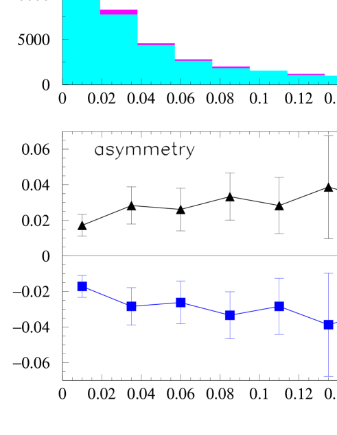
Figure 7: The asymmetry corresponding to the open upward triangles and open squares in Fig. 6, is shown in the $0<x_{2}<0.2$ range with a finer binning.

In Fig. 7, we show a finer binning of the range $0<x_{2}<0.2$ for the asymmetry obtained with the parametrization (12) for $100\,000$ events in the $4<M<9$ GeV case. It is a closer view of the very tiny error bars of open upward triangles and squares in Fig. 6. This is a peculiar feature of this parametrization, which emphasizes the role of very low $x_{2}$ through the parameters in Tab. 1, as it is discussed in Sec. III.0.1.

V Conclusions

In this paper, we have concentrated on the investigation of the spin structure of the proton using the single-polarized Drell-Yan process $pp^{\uparrow}\to\mu^{+}\mu^{-}X$. At leading twist, the cross section contains several terms that lead to an asymmetric distribution of the final muon pair in its azimuthal angle $\phi$ with respect to the production plane. In previous papers Bianconi and Radici (2005a, b), we considered those terms involving the transversity distribution $h_{1}$ and the Boer-Mulders function $h_{1}^{\perp}$ Boer (1999), which is believed to be responsible for the very well known violation of the Lam-Tung sum rule in the unpolarized Drell-Yan data Falciano et al. (1986); Guanziroli et al. (1988); Conway et al. (1989). There, we set up a Monte Carlo to numerically simulate (polarized) antiproton-proton Drell-Yan collisions to study the best kinematic conditions for the HESR at GSI Maggiora et al. (2005); Lenisa et al. (2004) that allow to extract unambiguous information on the target parton distributions.

Here, we have followed the same approach to isolate the contribution of the term involving the Sivers function $f_{1T}^{\perp}$, a ”naive T-odd” TMD partonic density that describes how the distribution of unpolarized quarks is distorted by the transverse polarization of the parent hadron. As such, $f_{1T}^{\perp}$ contains unsuppressed information on the orbital motion of hidden confined partons; better, it contains information on their spatial distribution Burkardt and Hwang (2004), and it offers a natural link between microscopic properties of confined elementary constituents and hadronic measurable quantities, such as the nucleon anomalous magnetic moment Burkardt and Schnell (2005). Factorization theorems for TMD distribution and fragmentation functions indicate that $f_{1T}^{\perp}$ is universal modulo a sign change (when switching from the SIDIS to the Drell-Yan process), due to a peculiar feature under the time-reversal operation of the gauge link operator required to make its definition color-gauge invariant Collins (2002).

Recently, very precise data for SSA involving $f_{1T}^{\perp}$ (the Sivers effect) have been obtained for the SIDIS process on transversely polarized protons Diefenthaler (2005). This allowed for more realistic parametrizations of $f_{1T}^{\perp}$ Anselmino et al. (2005a); Vogelsang and Yuan (2005); Collins et al. (2005a), that have been used then to make predictions for SSA in proton-proton collisions at RHIC (for a comparison among the various approaches, see also Ref. Anselmino et al. (2005b)).

Here, we have numerically simulated the Sivers effect for the $pp^{\uparrow}\to\mu^{+}\mu^{-}X$ process at $\sqrt{s}=200$ GeV including the foreseen upgrade in the RHIC luminosity (RHIC II). The goal is to explore the sensitivity of the simulated asymmetry to different input parametrizations, as well as to directly verify, within the reached statistical accuracy, the predicted sign change in the universality properties of the Sivers function. Therefore, we have employed the parametrization of Ref. Anselmino et al. (2005a) and a new high-energy parametrization of $f_{1T}^{\perp}$, whose flavor-dependent normalization and $p_{\scriptscriptstyle T}$ distribution are constrained by recent RHIC data on SSA for the $pp^{\uparrow}\to\pi X$ process at $\sqrt{s}=200$ GeV Adler et al. (2005). The main difference is that the former, fitted to the SIDIS data of Ref. Diefenthaler (2005), displays an emphasized relative importance of the unfavoured $d$ quark, and it gives an average transverse momentum $\langle q_{\scriptscriptstyle T}\rangle$ of the lepton pair much lower than the latter. Consistently, we have built spin asymmetries by integrating the $q_{\scriptscriptstyle T}$ distribution with adequate cutoffs, namely $0.1<q_{\scriptscriptstyle T}<2$ GeV/$c$ for the former parametrization, and $1<q_{\scriptscriptstyle T}<3$ GeV/$c$ for the latter. Results have been presented as binned in the parton momenta $x_{2}$ of the polarized proton, i.e. by integrating also upon the antiparton partner momenta $x_{1}$ and the zenithal muon pair distribution $\theta$ with no further cuts.

Sorted events are divided in two groups, corresponding to opposite azimuthal orientations of the muon pair with respect to the reaction plane (conventionally indicated with $U$ and $D$), and the asymmetry $(U-D)/(U+D)$ has been considered. Two different samples of $20\,000$ and $100\,000$ events have been selected, and statistical errors for $(U-D)/(U+D)$ have been obtained by making 10 independent repetitions of the simulation for each individual case and, then, calculating for each $x_{2}$ bin the average asymmetry and the variance. We have considered two different ranges of muon pair invariant mass, namely $4<M<9$ GeV and $12<M<40$ GeV. In this way, we avoid overlaps with the resonance regions of the $\bar{c}c$ and $\bar{b}b$ quarkonium systems, and we can safely assume that the elementary annihilation proceeds through the $\bar{q}q\to\gamma^{\ast}$ mechanism. In particular, the Monte Carlo is based on the corresponding leading-twist cross section. In the higher mass range, this theoretical analysis appears well established, since higher twists may be suppressed as $M_{p}/M$, where $M_{p}$ is the proton mass. More questionable is the case of the lower $M$ range, but this uncertainty can be traded for the much higher statistics that can be reached because of the $1/M^{2}$ contribution of the $\gamma^{\ast}$ propagator. Indeed, approximately 95% of the events fall in the $4<M<9$ GeV range with a significant reduction of the running time necessary to reach a predefined statistical accuracy.

More generally, a very small portion of the phase space, corresponding to the lowest possible values of $\tau=x_{1}x_{2}=M^{2}/s$, contains most of the events, also because of the high cm square energy $s$; typically, $\langle x_{1/2}\rangle\sim 0.01$. This is emphasized by the fact that in $pp$ collisions at least one of the two annihilating partons comes from the proton sea distribution, which is peaked at very low $x$ values. The importance of parton momenta below the valence region is potentially relevant to the theoretical models. In our case, it turns out that the parametrization of Ref. Anselmino et al. (2005a) gives small asymmetries because the emphasized unfavoured $\bar{d}d$ annihilation is statistically suppressed. As a consequence, in the $12<M<40$ GeV range $20\,000$ events are not sufficient to produce a Sivers effect that is not statistically consistent with zero. On the contrary, with the high-energy parametrization described in this paper this analysis is possible in the range $0<x_{2}\lesssim 0.5$, and a direct test of the ”universal” sign change of $f_{1T}^{\perp}$ can be unambiguously performed.

A more favourable situation is encountered with lower $M$ values, say in the $4<M<9$ GeV range. The much higher statistics significantly reduces the error bars and allows for a very short running time, typically as short as few days to collect the $100\,000$ events simulated here at the foreseen luminosity of $10^{32}$ cm^-2 sec^-1, irrespectively of the choice of input parametrizations for $f_{1T}^{\perp}$. Moreover, we observe that in the $0<x_{2}\lesssim 0.5$ range the two choices give two clearly distinct asymmetries, and for each case the results with opposite signs in the Sivers function can be unambiguously separated. Remarkably, we stress that this analysis holds also at very low $x_{2}$ values, typically as low as 0.01, which are relevant at RHIC.

In conclusion, at the foreseen luminosity of $10^{32}$ cm^-2 sec^-1 (RHIC II) and with a dilution factor 0.5, in few days RHIC can collect $100\,000$ Drell-Yan events for the process $pp^{\uparrow}\to\mu^{+}\mu^{-}X$ at $\sqrt{s}=200$ GeV and with muon pair invariant masses in the $4<M<9$ GeV range. From the measured Sivers effect, it should be possible to extract information on the $x$ structure of the Sivers function in the $0<x\lesssim 0.5$ range, particularly also at very low $x\sim 0.01$, as well as to test its ”universal” sign change predicted in Ref. Collins (2002). At higher $M$ values, like $12<M<40$ GeV, the situation is theoretically more favourable because the higher twists are suppressed as $1/M$. However, the lower density in the phase space makes the running time much longer. It is still possible to perform the previous analysis with $100\,000$ events and to come to the same conclusions, but at the price of taking data for some months. With a reduced sample, e.g. of $20\,000$ events, this time is shortened to few weeks, but our analysis was possible for only one of the chosen parametrizations, the other one giving results compatible with zero.