Reconstructing Supersymmetry at ILC/LHC

Abstract

DESY 05–240

IFIC/05–64

ZH–TH 25/05

Coherent analyses of experimental results from LHC and ILC will allow us to draw a comprehensive and precise picture of the supersymmetric particle sector. Based on this platform the fundamental supersymmetric theory can be reconstructed at the high scale which is potentially close to the Planck scale. This procedure will be reviewed for three characteristic examples: minimal supergravity as the paradigm; a left-right symmetric extension incorporating intermediate mass scales; and a specific realization of string effective theories.

1 Introduction

It is widely accepted that particle physics is rooted at the Planck scale where it is intimately linked with gravity. A stable bridge between the two vastly different scales, the electroweak scale of order 100 GeV and the grand unification / Planck scale of order $10^{16}$ / $10^{19}$ GeV, is built by supersymmetry which is characterized by a typical scale of order TeV. If this picture is realized in nature, methods must be developed which allow us to reconstruct the fundamental physics scenario near the grand unification / Planck scale. Elements of the picture can be provided by experiments observing proton decay, neutrino physics within the seesaw frame, various aspects of cosmology and, last not least, high-precision experiments at high energies [1].

The reconstruction of a physical scenario more than fourteen orders of magnitude above accelerator energies is a demanding task. Nevertheless, the extrapolation of the gauge couplings to the grand unification scale by renormalization group methods is an encouraging example [3]. In supersymmetric theories a rich ensemble of soft breaking parameters can be investigated. Symmetries and the impact of high-scale parameters can be studied which will reveal essential elements of the fundamental physics scenario [4].

The proton-collider LHC and the $e^{+}e^{-}$ linear collider ILC, now in the design phase, are a perfect tandem for exploring supersymmetry. The heavy colored supersymmetric particles, squarks and gluinos, can be generated for masses up to 3 TeV with large rates at LHC. Subsequent cascade decays give access to lower mass particles [5]. The properties of the potentially lighter non-colored particles, charginos/neutralinos and sleptons, can be studied very precisely at an $e^{+}e^{-}$ linear collider [6] by exploiting in particular polarization phenomena at such a lepton facility [7]. After the properties of the light particles are determined precisely, the properties of the heavier particles can subsequently be studied in the cascade decays with similar precision. Coherent LHC and ILC analyses [1] will thus provide us with a comprehensive and high-precision picture of supersymmetry at the electroweak scale, defining a solid platform for the reconstruction of the fundamental supersymmetric theory near the Planck scale.

This procedure will be described for three characteristic examples in this report – minimal supergravity, a left-right symmetric extension, and a string effective theory.

(a) Minimal supergravity [mSUGRA] [8] defines a scenario in which these general ideas can be quantified most easily due to the rather simple structure of the theory. Supersymmetry is broken in a hidden sector and the breaking is transmitted to our eigen-world by gravity. This suggests the universality of the soft SUSY breaking parameters – gaugino / scalar masses and trilinear couplings – at the high scale which is generally identified with the grand unification scale of the gauge couplings.

(b) Left-right symmetric extension: If in LR supersymmetric theories [9] non-zero neutrino masses are introduced by means of the seesaw mechanism [10], intermediate scales associated with the righ-handed neutrino masses of order $10^{10}$ to $10^{14}$ GeV affect the evolution of the supersymmetry parameters from the electroweak to the unification scale [11, 4]. If combined with universality at the unification scale, the intermediate scale modifies the observable scalar mass parameters in the lepton sector of the third generation at the electroweak scale. This effect can be exploited to estimate the seesaw scale [12], thus giving indirectly experimental access to the fundamental high-scale parameter in the neutrino sector.

(c) String effective theory: In orbifold compactifications of heterotic string theories, the universality of the scalar mass parameters is broken if these masses are generated by interactions with moduli fields [13]. Since the interactions are determined by modular weights that are integer numbers, the pattern of scalar masses is characteristic for such a scenario [4]. Thus this type of string theories can be tested stringently by measuring the modular weights.

2 Minimal Supergravity

The mSUGRA reference point SPS1a^′ [14], a derivative of the Snowmass point SPS1a [15], is characterized by the following values of the soft parameters at the grand unfication scale:

$$\begin{array}[]{ll}M_{1/2}=250~{}{\rm GeV}&M_{0}=70~{}{\rm GeV}\\ A_{0}=-300~{}{\rm GeV}&{\rm sign}(\mu)=+\\ \tan\beta=10&\\ \end{array}$$ (4)

The universal gaugino mass is denoted by $M_{1/2}$, the scalar mass by $M_{0}$ and the trilinear coupling by $A_{0}$; the sign of the higgsino mass parameter is chosen positive and $\tan\beta$, the ratio of the vacuum-expectation values of the two Higgs fields, in the medium range. The modulus of the higgsino mass parameter is fixed by requiring radiative electroweak symmetry breaking so that finally $\mu=+396$ GeV. The form of the supersymmetric mass spectrum in SPS1a^′ is shown in Fig. 1. In this scenario the squarks and gluinos can be studied very well at the LHC while the non-colored gauginos and sleptons can be analyzed partly at LHC and in comprehensive and precise form at an $e^{+}$e^- linear collider operating at a total energy up to 1 TeV with high integrated luminosity of 1 ab^-1.

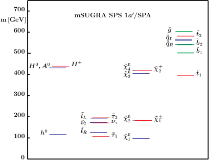
Figure 1: Supersymmetric mass spectrum for SPS1a’ scenario.

At LHC the masses can best be obtained by analyzing edge effects in the cascade decay spectra [16]. The basic starting point is the identification of a sequence of two-body decays: $\tilde{q}_{L}\rightarrow\tilde{\chi}^{0}_{2}q\rightarrow\tilde{\ell}_{R}\ell q\rightarrow\tilde{\chi}^{0}_{1}\ell\ell q$. The kinematic edges and thresholds predicted in the invariant mass distributions of the two leptons and the jet determine the masses in a model-independent way. The four sparticle masses [$\tilde{q}_{L}$, $\tilde{\chi}^{0}_{2}$, $\tilde{\ell}_{R}$ and $\tilde{\chi}^{0}_{1}$] are used subsequently as input for additional decay chains like $\tilde{g}\rightarrow\tilde{b}_{1}b\rightarrow\tilde{\chi}^{0}_{2}bb$, and the shorter chains $\tilde{q}_{R}\rightarrow q\tilde{\chi}^{0}_{1}$ and $\tilde{\chi}^{0}_{4}\rightarrow\tilde{\ell}\ell$, which all require the knowledge of the sparticle masses downstream of the cascades. Residual ambiguities and the strong correlations between the heavier masses and the LSP mass are resolved by adding the results from ILC measurements which improve the picture significantly.

Figure 2: Excitation curve for $e^{-}e^{-}\to\tilde{e}_{R}^{-}\tilde{e}_{R}^{-}$ near threshold, including background, initial-state radiation, beamstrahlung and Couloumb correction. The cross-section rises steeply in S-wave production. Ref. [18].

At ILC very precise mass values can be extracted from threshold scans and decay spectra [17]. The excitation curves for chargino production in S-waves rise steeply with the velocity of the particles near the thresholds and they are thus very sensitive to their mass values; the same holds true for mixed-chiral selectron pairs in $e^{+}e^{-}\to\tilde{e}_{R}^{+}\tilde{e}_{L}^{-}$ and for diagonal pairs in $e^{-}e^{-}\to\tilde{e}_{R}^{-}\tilde{e}_{R}^{-},\;\tilde{e}_{L}^{-}\tilde{e}_{L}^{-}$ collisions, cf. Fig. 2. Other scalar sfermions, as well as neutralinos, are produced generally in P-waves, with a less steep threshold behavior proportional to the third power of the velocity. Additional information, in particular on the lightest neutralino $\tilde{\chi}^{0}_{1}$, can be obtained from the very sharp edges of 2-body decay spectra, such as ${\tilde{l}}^{-}_{R}\to l^{-}{\tilde{\chi}}^{0}_{1}$, cf. Fig. 3.

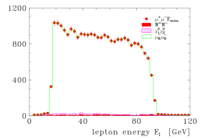
Figure 3: Energy sprectum of the muon from the decay ${\tilde{\mu}}^{-}_{R}\to\mu^{-}{\tilde{\chi}}^{0}_{1}$, with important backgrounds and including initial-state radiation and beamstrahlung effects. Ref. [19].

The values of typical mass parameters and their related measurement errors are presented in Tab. 1: “LHC” from LHC analyses and ”ILC” from ILC analyses. The third column “LHC+ILC” presents the corresponding errors if the experimental analyses are performed coherently, i.e. the light particle spectrum, studied at ILC with high precision, is used as input set for the LHC analysis.

$\begin{array}[]{|c|c||c|c||c|}\hline\cr\ \mbox{Particle}&\ \ \mbox{Mass}&\mbox{``LHC''}&\mbox{``ILC''}&\mbox{``LHC+ILC''}\\ \hline\cr\hline\cr h^{0}&116.9&0.25&0.05&0.05\\ H^{0}&425.0&&1.5&1.5\\ \hline\cr\tilde{\chi}^{0}_{1}&97.7&4.8&0.05&0.05\\ \tilde{\chi}^{0}_{2}&183.9&4.7&1.2&0.08\\ \tilde{\chi}^{0}_{4}&413.9&5.1&3-5&2.5\\ \tilde{\chi}^{\pm}_{1}&183.7&&0.55&0.55\\ \hline\cr\tilde{e}_{R}&125.3&4.8&0.05&0.05\\ \tilde{e}_{L}&189.9&5.0&0.18&0.18\\ \tilde{\tau}_{1}&107.9&5-8&0.24&0.24\\ \hline\cr\tilde{q}_{R}&547.2&7-12&-&5-11\\ \tilde{q}_{L}&564.7&8.7&-&4.9\\ \tilde{t}_{1}&366.5&&1.9&1.9\\ \tilde{b}_{1}&506.3&7.5&-&5.7\\ \hline\cr\tilde{g}&607.1&8.0&-&6.5\\ \hline\cr\end{array}$

Table 1: Accuracies for representative mass measurements of SUSY particles in individual LHC, ILC and coherent “LHC+ILC” analyses for the reference point SPS1a^′ [masses in GeV]. $\tilde{q}_{R}$ and $\tilde{q}_{L}$ represent the flavors $q=u,d,c,s$. [Errors presently extrapolated from SPS1a simulations.]

Mixing parameters must be extracted from measurements of cross sections and polarization asymmetries, in particular from the production of chargino pairs and neutralino pairs, both in diagonal or mixed form [20]: $e^{+}e^{-}\rightarrow{\tilde{\chi}^{+}_{i}}{\tilde{\chi}^{-}_{j}}$ [$i$,$j$ = 1,2] and ${\tilde{\chi}^{0}_{i}}{\tilde{\chi}^{0}_{j}}$ [$i$,$j$ = 1,$\dots$,4]. The production cross sections for charginos are binomials of $\cos\,2\phi_{L,R}$, the mixing angles rotating current to mass eigenstates. Using polarized electron and positron beams, the mixings can be determined in a model-independent way.

The fundamental SUSY parameters can be derived to lowest order in analytic form [20]:

$$\left|\mu\right| =M_{W}[\Sigma+\Delta[\cos 2\phi_{R}+\cos 2\phi_{L}]]^{1/2}$$

$$M_{2} =M_{W}[\Sigma-\Delta(\cos 2\phi_{R}+\cos 2\phi_{L})]^{1/2}$$

$$|M_{1}| =\left[\textstyle\sum_{i}m^{2}_{\tilde{\chi}_{i}^{0}}-M^{2}_{2}-\mu^{2}-2M^{2}_{Z}\right]^{1/2}$$

$$|M_{3}| =m_{\tilde{g}}$$

$$\tan\beta =\left[\frac{1+\Delta(\cos 2\phi_{R}-\cos 2\phi_{L})}{1-\Delta(\cos 2\phi_{R}-\cos 2\phi_{L})}\right]^{1/2}$$ (5)

where $\Delta=(m^{2}_{\tilde{\chi}^{\pm}_{2}}-m^{2}_{\tilde{\chi}^{\pm}_{1}})/(4M^{2}_{W})$ and $\Sigma=(m^{2}_{\tilde{\chi}^{\pm}_{2}}+m^{2}_{\tilde{\chi}^{\pm}_{1}})/(2M^{2}_{W})-1$. The signs of $\mu$, $M_{1,3}$ relative to $M_{2}$ follow from similar relations and from cross sections for ${\tilde{\chi}}$ production and $\tilde{g}$ processes.

The mass parameters of the sfermions are directly related to the physical masses if mixing effects are negligible:

$$m^{2}_{\tilde{f}_{L,R}}=M^{2}_{L,R}+m^{2}_{f}+D_{L,R}$$ (6)

with $D_{L}=(T_{3}-e_{f}\sin^{2}\theta_{W})\cos 2\beta\,m^{2}_{Z}$ and $D_{R}=e_{f}\sin^{2}\theta_{W}\cos 2\beta\,m^{2}_{Z}$ denoting the D-terms. The non-trivial mixing angles in the sfermion sector of the third generation follow from the sfermion production cross sections [21] for longitudinally polarized e⁺/e^- beams, which are bilinear in $\cos$/$\sin 2\theta_{\tilde{f}}$. The mixing angles and the two physical sfermion masses are related to the tri-linear couplings $A_{f}$, the higgsino mass parameter $\mu$ and $\tan\beta(\cot\beta)$ for down(up) type sfermions by:

$$A_{f}-\mu\tan\beta(\cot\beta)=\frac{m^{2}_{\tilde{f}_{1}}-m^{2}_{\tilde{f}_{2}}}{2m_{f}}\sin 2\theta_{\tilde{f}}$$ (7)

$A_{f}$ may be determined in the $\tilde{f}$ sector if $\mu$ has been measured in the chargino sector. This procedure can be applied in the stop sector. Heavy Higgs $H,A$ decays to stau pairs may be used to determine the $A$ parameter in the stau sector [22].

Refined analysis programs have been developed which include one-loop corrections in determining the Lagrangian parameters from masses and cross sections [23, 24] (see also [r22A]).

These measurements define the initial values for the evolution of the gauge couplings and the soft SUSY breaking parameters to the grand unification scale. The values at the electroweak scale are connected to the fundamental parameters at the GUT scale by the renormalization group equations. To leading order,
gauge couplings : $\alpha_{i}=Z_{i}\,\alpha_{U}$ (5) gaugino masses : $M_{i}=Z_{i}\,M_{1/2}$ (6) scalar masses : $\hskip 28.45274ptM^{2}_{\tilde{\jmath}}=M^{2}_{0}+c_{j}M^{2}_{1/2}+\sum_{\beta=1}^{2}c^{\prime}_{j\beta}\Delta M^{2}_{\beta}$ (7) trilinear couplings : $A_{k}=d_{k}A_{0}+d^{\prime}_{k}M_{1/2}$ (8) The index $i$ runs over the gauge groups $i=SU(3)$, $SU(2)$, $U(1)$. To this order, the gauge couplings, and the gaugino and scalar mass parameters of soft–supersymmetry breaking depend on the $Z$ transporters

$$Z_{i}^{-1}=1+b_{i}\frac{\alpha_{U}}{4\pi}\log\left(\frac{M_{U}}{M_{Z}}\right)^{2}$$ (12)

with $b[SU_{3},SU_{2},U_{1}]=-3,\,1,\,33/5$; the scalar mass parameters depend also on the Yukawa couplings $h_{t}$, $h_{b}$, $h_{\tau}$ of the top quark, bottom quark and $\tau$ lepton. The coefficients $c_{j}$ for the slepton and squark doublets/singlets, and for the two Higgs doublets, are linear combinations of the evolution coefficients $Z$; the coefficients $c^{\prime}_{j\beta}$ are of order unity. The shifts $\Delta M^{2}_{\beta}$, depending implicitly on all the other parameters, are nearly zero for the first two families of sfermions but they can be rather large for the third family and for the Higgs mass parameters. The coefficients $d_{k}$ of the trilinear couplings $A_{k}$ [$k=t,b,\tau$] depend on the corresponding Yukawa couplings and they are approximately unity for the first two generations while being O($10^{-1}$) and smaller if the Yukawa couplings are large; the coefficients $d^{\prime}_{k}$, depending on gauge and Yukawa couplings, are of order unity. Beyond the approximate solutions, the evolution equations have been solved numerically in the present analysis to two–loop order [26] and the threshold effects have been incorporated at the low scale in one-loop order [27]. Solutions of the renormalization group equations have been obtained meanwhile up to three-loop order [28], matching the new two-loop order results of the threshold corrections [29]. The 2-loop effects as given in Ref. [30] have been included for the neutral Higgs bosons and the $\mu$ parameter.

2.1 Gauge Coupling Unification

Measurements of the gauge couplings at the electroweak scale support very strongly the unification of the couplings at a scale $M_{U}\simeq 2\times 10^{16}$ GeV [3]. The precision, at the per–cent level, is surprisingly high after extrapolations over fourteen orders of magnitude in the energy from the electroweak scale to the grand unification scale $M_{U}$. Conversely, the electroweak mixing angle has been predicted in this approach at the per–mille level. The evolution of the gauge couplings from low energies to the GUT scale $M_{U}$ has been carried out at two–loop accuracy in the $\overline{DR}$ scheme. The gauge couplings do not meet exactly, cf. Fig. 4 and Tab. 2. The differences are to be attributed to high-threshold effects at the unification scale $M_{U}$ and the quantitative evolution implies important constraints on the particle content at $M_{U}$ [31].

a)                                                                       b)
                       

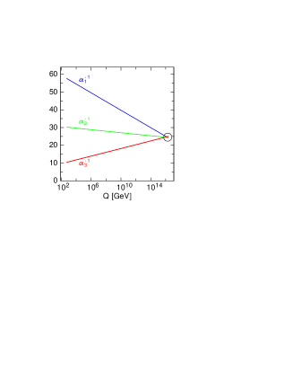
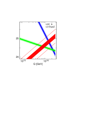
Figure 4: (a) Running of the inverse gauge couplings. (b) Close-up of the unification region. The thin lines represent uncertainties based on present data, the solid areas demonstrate the improvement expected by future GigaZ analyses.

	Present/”LHC”	GigaZ/”LHC+LC”
$M_{U}$	$(2.36\pm 0.06)\cdot 10^{16}\,\rm{GeV}$	$(2.360\pm 0.016)\cdot 10^{16}\,\rm{GeV}$
$\alpha_{U}^{-1}$	$24.19\pm 0.10$	$24.19\pm 0.05$
$\alpha_{3}^{-1}-\alpha_{U}^{-1}$	$0.97\pm 0.45$	$0.95\pm 0.12$

Table 2: Precision of extraction of the unified gauge coupling $\alpha_{U}$, derived from the meeting point of $\alpha_{1}$ with $\alpha_{2}$, and the strong coupling $\alpha_{3}$ at the GUT scale $M_{U}$. The columns demonstrate the results for the expected precision from LEP and LHC data, as well as the improvement due to a GigaZ linear collider analysis.

2.2 Gaugino and Scalar Mass Parameters

The results for the evolution of the mass parameters from the electroweak scale to the GUT scale $M_{U}$ are shown in Fig. 5. On the left of Fig. 5 the evolution is presented for the gaugino parameters $M^{-1}_{i}$. It clearly is under excellent control for the model-independent reconstruction of the parameters and the test of universality in the $SU(3)\times SU(2)\times U(1)$ group space. In the same way the evolution of the scalar mass parameters can be studied, presented in Fig. 5 (b) for the first/second generation. While the slepton parameters can be determined very accurately, the accuracy deteriorates for the squark parameters and the Higgs parameter $M^{2}_{H_{2}}$.

Figure 5: Evolution, from low to high scales, of (a) gaugino mass parameters and (b) first-generation sfermion mass parameters and the Higgs mass parameter $M^{2}_{H_{2}}$.

3 Left-right symmetric extension

The complex structure observed in the neutrino sector has interesting consequences for the properties of the sneutrinos, the scalar supersymmetric partners of the neutrinos. These novel elements require the extension of the minimal supersymmetric Standard Model MSSM, e.g., by a superfield including the right-handed neutrino field and its scalar partner [9]. If the small neutrino masses are generated by the seesaw mechanism [10], a similar type of spectrum is induced in the scalar sector, splitting into light TeV-scale and very heavy masses. The intermediate seesaw scales will affect the evolution of the soft mass terms which break the supersymmetry at the high (GUT) scale, particularly in the third generation with large Yukawa couplings [4, 12]. This will provide the opportunity to measure, indirectly, the intermediate seesaw scale of the third generation.

If sneutrinos are lighter than charginos and the second lightest neutralino, as encoded in SPS1a^′, they decay only to final states ${\tilde{\nu}_{l}}\to\nu_{l}\,\tilde{\chi}^{0}_{1}$ that are invisible and pair-production is useless for studying these particles. However, in this configuration sneutrino masses can be measured in chargino decays to sneutrinos and leptons [12]:

$$\tilde{\chi}^{\pm}_{1}\to l^{\pm}\,{\tilde{\nu}}_{l}^{(*)},$$ (13)

with the charginos pair-produced in $e^{+}e^{-}$ annihilation. These two-particle decays develop sharp edges at the endpoints of the lepton energy spectra. Sneutrinos of all three generations can be explored this way. The errors for the first and second generation sneutrinos are expected at the level of 400 MeV, doubling for the more involved analysis of the third generation.

The measurement of the seesaw scale will be illustrated in an SO(10) model in which the matter superfields of the three generations belong to 16-dimensional representations of SO(10) and the standard Higgs superfields to 10-dimensional representations while a Higgs superfield in the 126-dimensional representation generates Majorana masses for the right-handed neutrinos. As a result, the Yukawa couplings in the neutrino sector are proportional to the up-type quark mass matrix, for which the standard texture is assumed. The SO(10) symmetry is broken to the Standard Model SU(3)$\times$SU(2)$\times$U(1) symmetry at the grand unification scale $M_{U}$ directly. For simplicity the soft masses in the Higgs sector will be identified with the matter sector.

Assuming that the Yukawa couplings are the same for up-type quarks and neutrinos at the GUT scale and that the Majorana mass matrix of the right-handed neutrinos has a similar structure, one obtains a (weakly) hierarchical neutrino mass spectrum and nearly bi-maximal mixing for the left-handed neutrinos [32]. In this class of models the masses of the right-handed neutrinos are also hierarchical, very roughly $\propto m^{2}_{\rm up}$, and the mass of the heaviest neutrino is given by $M_{{\rm R}_{3}}\sim m^{2}_{t}/m_{\nu_{3}}$. For $m_{\nu_{3}}\sim 5\times 10^{-2}$ eV, the heavy neutrino mass of the third generation amounts to $\sim 6\times 10^{14}$ GeV, i.e. a value close to the grand unification scale $M_{U}$.

Figure 6: Evolution of third generation slepton mass parameters and Higgs mass parameters $M^{2}_{H_{2}}$ in LR-SUGRA.

Since the $\nu_{R}$ of the third generation is unfrozen only beyond $Q=M_{\nu_{R}}$ the impact of the LR extension becomes visible in the evolution of the scalar mass parameters only at very high scales. In Fig. 6 the evolution of $M^{2}_{\tilde{E}_{3}}$, $M^{2}_{\tilde{L}_{3}}$ and $M^{2}_{H_{2}}$ is displayed for illustrative purposes. The full lines include the effects of the right–handed neutrino, which should be compared with the dashed lines where the $\nu_{R}$ effects are removed. The scalar mass parameter $M^{2}_{\tilde{E}_{3}}$ appears unaffected by the right–handed sector, while $M^{2}_{\tilde{L}_{3}}$ and $M^{2}_{H_{2}}$ clearly are. Only the picture including $\nu_{R}$, $\tilde{\nu_{R}}$ is compatible with the unification assumption. The kinks in the evolution of $M^{2}_{{\tilde{L}}_{3}}$ and $M^{2}_{\tilde{H_{2}}}$ can be traced back to the fact that around $10^{14}$ GeV the third generation (s)neutrinos become quantum mechanically effective, given a large enough neutrino Yukawa coupling to influence the evolution of these mass parameters.

To leading order, the solutions of the renormalization group equations for the masses of the scalar selectrons and the $e$-sneutrino can be expressed by the high scale parameters $m_{16}$ and $M_{1/2}$, and the D-terms. Analogous representations can be derived, to leading order, for the scalar masses of the third generation, complemented however by additional contributions $\Delta_{\tau}$ and $\Delta_{\nu_{\tau}}$ from the standard tau Yukawa term and the Yukawa term in the tau neutrino sector, respectively:

$$m^{2}_{\tilde{\tau}_{R}} =m^{2}_{\tilde{e}_{R}}-2\Delta_{\tau}+m^{2}_{\tau}$$ (14)

$$m^{2}_{\tilde{\tau}_{L}} =m^{2}_{\tilde{e}_{L}}-\Delta_{\tau}-\Delta_{\nu_{\tau}}+m^{2}_{\tau},$$ (15)

$$m^{2}_{\tilde{\nu}_{\tau L}} =m^{2}_{\tilde{\nu}_{eL}}-\Delta_{\tau}-\Delta_{\nu_{\tau}}.$$ (16)

The contribution $\Delta_{\nu_{\tau}}=\Delta_{\nu_{\tau}}[M_{\rm R}]$ carries the information on the value of the heavy right-handed neutrino mass.

The effect of the right-handed neutrinos can be identified by evaluating the sum rule for the $\Delta_{\nu_{\tau}}$ parameter:

$$2\Delta_{\nu_{\tau}}[M_{{\rm R}_{3}}] =(3m^{2}_{\tilde{\nu}_{e{\rm L}}}-m^{2}_{\tilde{e}_{\rm L}}-m^{2}_{\tilde{e}_{\rm R}})$$ (17)

$$\,-(3m^{2}_{\tilde{\nu}_{\tau{\rm L}}}-m^{2}_{\tilde{\tau}_{1}}-m^{2}_{\tilde{\tau}_{2}})-2m_{\tau}^{2}.$$

This relation holds exactly at tree-level and gets modified slightly only by small corrections at the one-loop level. The particular form of eq. (17) implies that the effects of the $\tau$ Yukawa coupling cancel. It follows from the renormalization group equations that $\Delta_{\nu_{\tau}}[M_{{\rm R}_{3}}]$ is of the order $Y^{2}_{\nu}\log{M^{2}_{\rm GUT}/M^{2}_{{\rm R}_{3}}}$. Since the Yukawa coupling $Y_{\nu}$ can be estimated in the seesaw mechanism by the mass $m_{\nu_{3}}$ of the third light neutrino, $Y_{\nu}^{2}=m_{\nu_{3}}M_{{\rm R}_{3}}/(v\,\sin\beta)^{2}$, the parameter $\Delta_{\nu_{\tau}}[M_{R_{3}}]$ depends approximately linearly on the mass $M_{{\rm R}_{3}}$:

$$\Delta_{\nu_{\tau}}[M_{R_{3}}]\simeq \,\frac{m_{\nu_{3}}M_{{\rm R}_{3}}}{16\pi^{2}(v\,\sin\beta)^{2}}$$ (18)

$$\times\left(3m^{2}_{16}+A^{2}_{0}\right)\log\frac{M^{2}_{\rm GUT}}{M^{2}_{{\rm R}_{3}}},$$

so that it can be determined very well. Inserting the value for $m_{16}$, pre-determined in the charged slepton sector, and the trilinear coupling $A_{0}$ from stop mixing [21], $M_{{\rm R}_{3}}$, cf. Fig. 7, can finally be calculated.

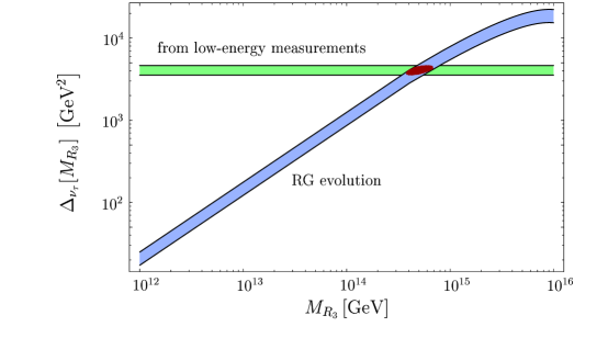
Figure 7: Shift $\Delta_{\nu_{\tau}}$ in the evolution of the tau-neutrino mass as calculated from the renormalization group equations, eq. (18) (blue band) and compared with low-energy mass measurements, eq. (17) (green band). The widths of the bands indicate estimated one-standard-deviations errors of the experimental input parameters. The red crossing region is the statistical combination which determines the neutrino seesaw scale $M_{{\rm R}_{3}}$ of the third generation.

Assuming hierarchical neutrino masses, one obtains

$$M_{{\rm R}_{3}}=3.7\;\dots\;6.9\times 10^{14}\,\,\mathrm{GeV},$$ (19)

to be compared with the initial value $M_{{\rm R}_{3}}=6\times 10^{14}$ GeV. This analysis thus provides us with a unique estimate of the high-scale $\nu_{R}$ mass parameter $M_{{\rm R}_{3}}$.

4 String Effective Theories

In the supergravity models analyzed above the supersymmetry breaking mechanism in the hidden sector is shielded from the eigen–world. Four–dimensional strings however give rise to a minimal set of fields for inducing supersymmetry breaking, the dilaton $S$ and the moduli $T$ superfields which are generically present in large classes of 4–dimensional heterotic string theories [13]. The vacuum expectation values of $S$ and $T$, generated by genuinely non–perturbative effects, determine the soft supersymmetry breaking parameters.

The properties of the supersymmetric theories are quite different for dilaton and moduli dominated scenarios. This can be quantified by introducing a mixing angle $\theta$, characterizing the $\tilde{S}$ and $\tilde{T}$ wave functions of the Goldstino, which is associated with the breaking of supersymmetry and which is absorbed to generate the mass of the gravitino: $\tilde{G}=\sin\theta\,\tilde{S}+\cos\theta\,\tilde{T}$. The mass scale is set by the second parameter of the theory, the gravitino mass $m_{3/2}$.

A dilaton dominated scenario, i.e. $\sin\theta\to 1$, leads to universal boundary conditions of the soft supersymmetry breaking parameters. Universality is broken only slightly by small loop effects. On the other hand, in moduli dominated scenarios, $\cos\theta\to 1$, the gaugino mass parameters are universal to lowest order, but universality is not realized for the scalar mass parameters. The breaking is characterized by modular weights $n_{j}$ which quantify the couplings between the matter and the moduli fields in orbifold compactifications. Within one generation significant differences between left and right field components and between sleptons and squarks can occur.

In leading order the masses [33] are given by the following expressions for the gaugino sector,

$$M_{i} = -g_{i}^{2}m_{3/2}s{\sqrt{3}\sin\theta}+...$$ (20)

and for the scalar sector,

$$M_{\tilde{j}}^{2} = m^{2}_{3/2}\left(1+n_{j}\cos^{2}\theta\right)+...$$ (21)

A mixed dilaton/moduli superstring scenario has been analyzed in detail with dominating dilaton component, $\sin^{2}\theta=0.9$, and with different couplings of the moduli field to the (L,R) sleptons, the (L,R) squarks and to the Higgs fields, corresponding to O–I representation $n_{L_{i}}=-3$, $n_{E_{i}}=-1$, $n_{H_{1}}=n_{H_{2}}=-1$, $n_{Q_{i}}=0$, $n_{D_{i}}=1$ and $n_{U_{i}}=-2$, an assignment that is adopted quite frequently in the literature. The gravitino mass is chosen to be 180 GeV in this analysis.

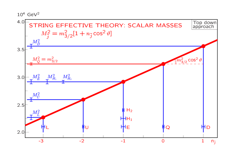
Figure 8: Extraction of parameters of superstring inspired supersymmetry breaking scenario from gaugino and scalar evolution.

Given this set of superstring induced parameters, the evolution of the gaugino and scalar mass parameters can be exploited to determine the modular weights $n$. The result is shown in Fig. 8 which demonstrates quite nicely how stringently this theory can be tested by analyzing the integer character of the entire set of weights.

Thus, high-precision measurements at high energy proton and $e^{+}e^{-}$ linear colliders provide access to crucial derivative parameters in string theories.

5 Conclusions

In supersymmetric theories stable extrapolations can be performed, by renormalization group techniques, from the electroweak scale to the grand unification scale close to the Planck scale. Such extrapolations are made possible by high-precision measurements of the low-energy parameters. In the near future an enormous corpus of information is expected to become available if measurements at LHC and prospective $e^{+}e^{-}$ linear colliders are combined to draw a comprehensive and high-precision picture of supersymmetric particles and their interactions.

Supersymmetric theories and their breaking mechanisms have simple structures at high scales. Extrapolations to these scales are therefore crucial to reveal the fundamental supersymmetric theory, including its symmetries and its parameters. The extrapolations can thus be used to explore physics phenomena at a scale where, eventually, particle physics is linked to gravity.

We have reviewed three interesting scenarios in this context. The universality of gaugino and scalar mass parameters in minimal supergravity can be demonstrated very clearly. Intermediate scales, like seesaw scales in left-right symmetric theories, affect the evolution of the scalar mass parameters. Their effect on the mass parameters of the third generation can be exploited to determine the seesaw scale. Finally it has been shown that integer modular weights can be measured accurately in string effective theories, scrutinizing such approaches quite stringently.

Many more refinements of the theoretical calculations and future experimental analyses will be necessary to expand the pictures we have described in this review. Prospects of exploring elements of the ultimate unification of the interactions provide a strong impetus to this endeavor.

References

- [1] B. C. Allanach, G. A. Blair, S. Kraml, H. U. Martyn, G. Polesello, W. Porod and P. M. Zerwas, hep-ph/0403133; short version to be published in [2].
- [2] LHC/LC Study Group Working Report, eds. G. Weiglein et al., hep-ph/0410364; Phys. Rep. C in preparation.
- [3] S. Dimopoulos, S. Raby and F. Wilczek, Phys. Rev. D 24 (1981) 1681; L. E. Ibáñez and G. G. Ross, Phys. Lett. B 105 (1981) 439; U. Amaldi, W. de Boer and H. Fürstenau, Phys. Lett. B 260 (1991) 447; P. Langacker and M. x. Luo, Phys. Rev. D 44 (1991) 817; J. R. Ellis, S. Kelley and D. V. Nanopoulos, Phys. Lett. B 260 (1991) 131.
- [4] G. A. Blair, W. Porod and P. M. Zerwas, Phys. Rev. D63 (2001) 017703 and Eur. Phys. J. C27 (2003) 263; P. M. Zerwas et al., Proceedings, Int. HEP Conf., Amsterdam 2002, hep-ph/0211076.
- [5] I. Hinchliffe et al., Phys. Rev. D 55, 5520 (1997); Atlas Collaboration, Technical Design Report 1999, Vol. II, CERN/LHC/99-15, ATLAS TDR 15.
- [6] TESLA Technical Design Report (Part 3), R. D. Heuer, D. J. Miller, F. Richard and P. M. Zerwas (eds.), DESY 010-11, hep-ph/0106315; American LC Working Group, T. Abe et al., SLAC-R-570 (2001), hep-ex/0106055-58; ACFA LC Working Group, K. Abe et al., KEK-REPORT-2001-11, hep-ex/0109166; CLIC Group, M. Battaglia, A. De Roeck, J. Ellis and D. Schulte (eds.), hep-ph/0412251.
- [7] LC Polarization Group, G. Moortgat-Pick et al., hep-ph/0507011, Phys. Rep. C in preparation.
- [8] A. H. Chamseddine, R. Arnowitt and P. Nath, Phys. Rev. Lett. 49 (1982) 970; H. P. Nilles, Phys. Rept. 110 (1984) 1.
- [9] K. S. Babu and R. N. Mohapatra, Phys. Rev. Lett. 70 (1993) 2845; for a review see: S. F. King, Rept. Prog. Phys. 67 (2004) 107.
- [10] P. Minkowski, Phys. Lett. B 67 (1977) 421; M. Gell-Mann, P. Ramond, and R. Slansky, in Proc. of the Workshop on Complex Spinors and Unified Theories, Stony Brook, New York, North-Holland, 1979; T. Yanagida, (KEK, Tsukuba), 1979; R. N. Mohapatra and G. Senjanovic, Phys. Rev. Lett. 44 (1980) 912.
- [11] H. Baer, C. Balázs, J. K. Mizukoshi and X. Tata, Phys. Rev. D 63 (2001) 055011.
- [12] A. Freitas, W. Porod and P. M. Zerwas, hep-ph/0509056.
- [13] M. Cvetič, A. Font, L. E. Ibáñez, D. Lust and F. Quevedo, Nucl. Phys. B 361 (1991) 194; A. Brignole, L. E. Ibáñez and C. Munoz, Nucl. Phys. B 422 (1994) 125 [Erratum-ibid. B 436 (1995) 747]; A. Love and P. Stadler, Nucl. Phys. B 515 (1998) 34.
- [14] Supersymmetry Parameter Analysis (SPA) Project, http://spa.desy.de/spa/; J. A. Aguilar-Saavedra et al., hep-ph/0511344.
- [15] B. C. Allanach et al., Eur. Phys. J. C 25 (2002) 113.
- [16] B. C. Allanach, C. G. Lester, M. A. Parker and B. R. Webber, JHEP 0009 (2000) 004; B. K. Gjelsten, D. J. Miller and P. Osland, JHEP 0412 (2004) 003 and B. K. Gjelsten, D. J. Miller and P. Osland, JHEP 0506 (2005) 015.
- [17] A. Freitas, H. U. Martyn, U. Nauenberg and P. M. Zerwas, in Proc. of the International Conference on Linear Colliders 2004, Paris, France, hep-ph/0409129.
- [18] A. Freitas, D. J. Miller and P. M. Zerwas, Eur. Phys. J. C21 (2001) 361; A. Freitas, A. von Manteuffel and P. M. Zerwas, Eur. Phys. J. C34 (2004) 487.
- [19] H. U. Martyn, contribution to 3rd Workshop of Extended ECFA/DEST LC Study, 2002, Prague, Czech Republic, LC-PHSM-2003-071, hep-ph/0406123.
- [20] S.Y. Choi, A. Djouadi, M. Guchait, J. Kalinowski, H.S. Song and P.M. Zerwas, Eur. Phys. J. C14 (2000) 535; S.Y. Choi, J. Kalinowski, G. Moortgat-Pick and P.M. Zerwas, Eur. Phys. J. C22 (2001) 563 and Eur. Phys. J. C23 (2002) 769.
- [21] A. Bartl, H. Eberl, S. Kraml, W. Majerotto and W. Porod, Eur. Phys. J. directC 2 (2000) 6; E. Boos, H. U. Martyn, G. Moortgat-Pick, M. Sachwitz, A. Sherstnev and P. M. Zerwas, Eur. Phys. J. C 30, 395 (2003).
- [22] S. Y. Choi, H. U. Martyn and P. M. Zerwas, hep-ph/0508021.
- [23] R. Lafaye, T. Plehn and D. Zerwas, hep-ph/0404282, in [2].
- [24] P. Bechtle, K. Desch and P. Wienemann, in Proc. of the International Linear Collider Workshop 2005, Stanford, California, USA, hep-ph/0506244.
- [25] J. Reuter et al., hep-ph/0512012.
- [26] S. Martin and M. Vaughn, Phys. Rev. D50, 2282 (1994); Y. Yamada, Phys. Rev. D50, 3537 (1994); I. Jack, D.R.T. Jones, Phys. Lett. B333 (1994) 372.
- [27] J. Bagger, K. Matchev, D. Pierce, and R. Zhang, Nucl. Phys. B491 (1997) 3.
- [28] I. Jack, D. R. T. Jones and A. F. Kord, Annals Phys. 316 (2005) 213.
- [29] S. P. Martin, Phys. Rev. D 71 (2005) 116004.
- [30] G. Degrassi, P. Slavich and F. Zwirner, Nucl. Phys. B611 (2001) 403; A. Brignole, G. Degrassi, P. Slavich and F. Zwirner, Nucl. Phys. B631 (2002) 195; Nucl. Phys. B643 (2002) 79; A. Dedes and P. Slavich, Nucl. Phys. B657 (2003) 333; A. Dedes, G. Degrassi and P. Slavich, Nucl. Phys. B 672 (2003) 144.
- [31] G.G. Ross and R.G. Roberts, Nucl. Phys. B377 (1992) 571.
- [32] W. Buchmüller and D. Wyler, Phys. Lett. B 521 (2001) 291.
- [33] P. Binetruy, M. K. Gaillard and B. D. Nelson, Nucl. Phys. B 604 (2001) 32.