DAMTP-2005-119
hep-th/0512081 Low-Energy Supersymmetry Breaking from String Flux Compactifications: Benchmark Scenarios

Abstract

Soft supersymmetry breaking terms were recently derived for type IIB string flux compactifications with all moduli stabilised. Depending on the choice of the discrete input parameters of the compactification such as fluxes and ranks of hidden gauge groups, the string scale was found to have any value between the TeV and GUT scales. We study the phenomenological implications of these compactifications at low energy. Three realistic scenarios can be identified depending on whether the Standard Model lies on D3 or D7 branes and on the value of the string scale. For the MSSM on D7 branes and the string scale between $10^{12}$ GeV and $10^{17}$ GeV we find that the LSP is a neutralino, while for lower scales it is the stop. At the GUT scale the results of the fluxed MSSM are reproduced, but now with all moduli stabilised. For the MSSM on D3 branes we identify two realistic scenarios. The first one corresponds to an intermediate string scale version of split supersymmetry. The second is a stringy mSUGRA scenario. This requires tuning of the flux parameters to obtain the GUT scale. Phenomenological constraints from dark matter, $(g-2)_{\mu}$ and $BR(b\rightarrow s\gamma)$ are considered for the three scenarios. We provide benchmark points with the MSSM spectrum, making the models suitable for a detailed phenomenological analysis.

1 Introduction

The minimal supersymmetric standard model (MSSM) has been subject to a vast amount of study during the past decades. Our ignorance of the mechanism of supersymmetry (SUSY) breaking as well as the messenger mechanism allows for a large number of free parameters and therefore different experimental signatures of supersymmetric models (for a review see [1]) .

Detailed studies regarding the concrete low energy spectrum and interactions have to be performed on very specific models. A handful of benchmark points were chosen [2, 3] in order to extract low energy implications that can be eventually contrasted with experiment. It is however desirable to have a top-down derivation of soft supersymmetry breaking terms, obtained from a fundamental theory such as string theory. This would provide a more robust theoretical motivation for selecting particular benchmark points.

Until recently this task was not fully possible because there were no explicit derivations of soft SUSY breaking terms from string theory (see, for example, [4]). Even though some general scenarios were identified, such as dilaton and moduli domination, there were no proper models in which all moduli were stabilised after SUSY breaking. Dramatic progress has been achieved in recent years regarding moduli stabilisation in flux compactifications. In the type IIB context these have been investigated in detail, with the result that a large class of moduli are stabilised by turning on fluxes of antisymmetric tensor fields. The remaining moduli, including the volume of the compact space, can be stabilised by nonperturbative effects, such as in the KKLT mechanism [5] and related generalisations.

Studies of soft SUSY breaking terms from fluxes were performed recently by several groups [6]. The phenomenological implications were explored in ref. [7]. However, these studies, while fixing all the complex structure moduli and the dilaton, did not stabilise the volume-like moduli. In the KKLT scenario the rest of the moduli are stabilised but the effect of SUSY breaking by fluxes is washed out by nonperturbative effects. The source of SUSY breaking is then the least understood part of the scenario corresponding to the introduction of explicit soft breaking from anti D3 branes. Furthermore, in this scenario, it has not been possible to perform a proper analysis of soft terms in concrete models due to technical complications in the stabilisation process. A phenomenological analysis of models inspired by the KKLT scenario was recently performed in [8, 9, 10, 11, 12].

Fortunately, a generalisation of the KKLT scenario was constructed recently [13], henceforth referred to as the large volume scenario, in which, for half of the Calabi-Yau compactifications, all moduli are stabilised. The salient feature of these models is that the Calabi-Yau volume is generically exponentially large, allowing for a range of values for the string scale (from TeV to the GUT scale). This is to be contrasted with the KKLT case in which the volume has only a logarithmic dependence on flux parameters and it is difficult to obtain a weakly coupled (large volume) model. Another important feature is that only one of the Kähler moduli is stabilised at a large value, whereas all others are $\;\raisebox{-3.00003pt}{$\stackrel{{\scriptstyle\displaystyle>}}{{\sim}}$}\;1.$ In ref. [14], masses of both bulk and brane moduli were explicitly computed. The moduli masses are dependent on two parameters - the Calabi-Yau volume, $\cal{V}$, which is expected to be large, and the flux superpotential $W_{0}$ which is generically ${\cal{O}}(1).$ Furthermore, unlike the original KKLT version, the $1/{\cal{V}}$ expansion allows for explicit control of the calculation of the soft breaking terms. These were derived in ref. [14] for the Calabi-Yau compactifications that admit the exponentially large volume minimum.

In this article we make a study of the phenomenological implications of the different scenarios that emerge from this general class of string compactifications. We will identify three semi-realistic scenarios as follows.

1. Generalised Fluxed MSSM. If the Standard Model lies on D7 branes, the discrete input parameters allow for string scales between the intermediate $10^{9}$GeV and the GUT scales. The models generically suffer from the cosmological moduli problem and smaller string scales ($<10^{11}$GeV) tend to lead to a stop lightest supersymmetric particle (LSP) instead of a neutralino. To leading order in $1/{\cal{V}}$ expansion, the GUT scale case reproduces the fluxed MSSM [15].

2. Intermediate Scale Split SUSY. If the Standard Model lives on a set of D3 branes, the scalar masses are naturally many orders of magnitude heavier than gaugino masses and for an intermediate string scale gaugino masses are of order TeV. Standard fine tuning is then needed to keep the Higgs light as in the split supersymmetry scenario. Thus we provide a stringy realisation of split SUSY.

3. Stringy mSUGRA. Tuning the value of the flux superpotential $W_{0}$ it is possible to obtain a string scale of order the GUT scale and all soft-breaking terms of the same order as in the standard mSUGRA scenario. Again, this provides a stringy realisation of this popular scenario.

In each case we perform an RG flow to low energies and impose phenomenological constraints from dark matter, $(g-2)_{\mu}$ and $BR(b\rightarrow s\gamma)$. Since the third scenario has been largely explored, we only provide detailed analysis for models within the first two scenarios, selecting benchmark points in which the full low-energy spectrum is computed. In the rest of the article we describe each of these scenarios, starting with a brief overview of the results in [14].

2 Moduli Stabilisation, Masses and Scales

Here we will mention the relevant properties of the KKLT/large volume compactifications that will be needed for the analysis of soft breaking terms.

Type IIB string models have the following bosonic spectrum of massless fields in 10d: the metric $g_{MN}$, two rank-two antisymmetric tensors $B_{MN},C_{MN}$, a complex dilaton/axion scalar $S=e^{-\phi}+ia$ and a rank-four antisymmetric tensor with self-dual field strength. A typical string compactification is determined by the following procedure:

• First turn on a background value of the metric to split the spacetime into our 4d spacetime and six extra compact dimensions which are taken to be a Calabi-Yau orientifold in order to preserve ${\cal{N}}=1$ supersymmetry in 4d. The Calabi-Yau space is characterised by the number of two-cycles and their dual four-cycles, as well as the number of three-cycles. The sizes of these cycles are in general arbitrary. They define the Kähler structure moduli $T$ for the size of the four and two cycles and complex structure moduli $U$ for the size of the three cycles. These moduli correspond to the internal components of the metric which in the 4d effective field theory appear as a set of massless scalar fields, clearly in contradiction with experiment. Fixing the vacuum expectation value of these fields while providing them a mass is the problem of moduli stabilisation in string theory.

• Turning on the other bosonic fields in the spectrum helps stabilise the complex structure moduli by the standard requirement of flux quantisation of the field strength of rank-two antisymmetric tensors. This also fixes the vacuum expectation values of the dilaton/axion field. Fluxes modify the geometry but in type IIB string theory the remnant space is a warped Calabi-Yau which is conformally equivalent to a Calabi-Yau. Therefore the usual properties of Calabi-Yau spaces can still be used in flux compactifications. This is not the case for the other string theories, such as the type IIA or heterotic string.

• These models generically have D-branes. D3 and D7 branes can be introduced while preserving supersymmetry. These play an important role because it is on the D-branes that the Standard Model can live. Branes cannot be introduced arbitrarily because of consistency (tadpole cancellation) conditions requiring the total charge of a given D-brane type to vanish due to the compactness of the internal manifold. We can consider the Standard Model matter being on either the D7 or D3 branes. There can also be hidden sector D3/D7 branes. These can induce non-perturbative superpotentials for the $T_{a}$ fields ($W_{np}\sim e^{-aT}$), completing the geometric moduli stabilisation process. Other moduli, corresponding to the position of the D7 branes within the Calabi-Yau manifold, can also be determined by the combined flux and non-perturbative superpotentials.

• The previous procedure usually fixes the moduli with a negative value of the cosmological constant. There are several proposals for lifting the minimum of the scalar potential to a zero or positive vacuum energy, such as the inclusion of anti D3 branes [5], D-terms [16], IASD fluxes [17], etc.

Only after all moduli have been stabilised is a vacuum obtained for which the physical properties of the particles (in particular the soft SUSY breaking terms) in the spectrum may be analysed. Therefore, phenomenological analysis relies heavily on moduli stabilisation. In the past, it was simply assumed that moduli were stabilised, without providing a mechanism.

In the KKLT scenario and recent modifications moduli stabilisation is possible. We will consider the large volume scenario described in the introduction since it allows for explicit minima of the scalar potential at large enough volumes to trust the effective field theory treatment. An important property of this scenario is that, contrary to the KKLT case, the main source of supersymmetry breaking are the fluxes and not the ad hoc introduction of anti D3 branes or D-terms.

The input parameters are:

1. The flux superpotential $W_{0}$. It depends on combinations of integers determined by the fluxes. Statistically it can take any value but very small values ($\sim 10^{-11}$) are difficult to obtain. This is usually described as ‘fine-tuning’ of flux superpotentials.

2. The string coupling constant $g_{s}$. This corresponds to the vacuum expectation value (vev) of the dilaton field $S$ and it is determined by the fluxes. Values of order $1/10$ are easy to obtain.

3. The volume of the Calabi-Yau $\cal{V}$ which is a combination of the $T$ moduli. It is determined primarily by an exponential dependence on the rank of the hidden sector gauge group and the string coupling constant.

4. Warp factors of the metric at the location of the D branes. These play a role in tuning the minimum to de Sitter space. They may also play a role in redshifting scales in the Standard Model brane.

The string scale and the gravitino mass are determined in terms of $W_{0}$ and $\cal{V}$ by

$$m_{s} = \frac{g_{s}}{\sqrt{4\pi{\cal{V}}}}M_{P},$$ (1)

$$m_{3/2} = \frac{g_{s}^{2}W_{0}}{\sqrt{4\pi}{\cal{V}}}M_{P},$$ (2)

respectively. Here $g_{s}$ denotes the string coupling and $M_{P}=2.4\times 10^{18}$GeV is the reduced Planck mass. Table 1 shows the dependence of D3 soft terms on $W_{0}$ and $\cal{V}.$

Quantity	Order of magnitude
Scalar masses $m_{i}$	$\frac{g_{s}^{2}}{({\cal{V}})^{7/6}}W_{0}M_{P}$
Gaugino masses $M_{D3}$	$\frac{g_{s}^{2}}{({\cal{V}})^{2}}W_{0}M_{P}$
Scalar trilinear coupling $A$	$\frac{g_{s}^{2}}{({\cal{V}})^{4/3}}W_{0}M_{P}$
$\mu$-term $\hat{\mu}$	$\frac{g_{s}^{2}}{({\cal{V}})^{4/3}}W_{0}M_{P}$
B term $\hat{\mu}B$	$\frac{g_{s}^{2}}{({\cal{V}})^{7/3}}W_{0}M_{P}$

Table 1: Soft terms for D3 branes (AMSB contributions not included).

In the original KKLT model the value of $W_{0}$ had to be very small (typically of order $10^{-4}-10^{-11}$) in order to obtain a minimum within the supergravity approximation. In the scenario of [13, 14], this is not needed and moduli can be stabilised with the generic case $W_{0}\approx 1$. There is, however, still some freedom to tune $W_{0}$ in order to explore possible realistic models.

Table 2 shows the masses of bulk moduli for a range of string scales, as derived in [14]. $W_{0}$ is taken to be equal to 1. Note that complex structure and most of the Kähler moduli, $\tau_{s}$, have masses comparable to the gravitino mass, while the modulus with the exponentially large value $\tau_{b}$ is much lighter.

String scale $m_{s}$	complex structure, $\tau_{s}$	$\tau_{b}$ (lightest bulk modulus)
$10^{3}$GeV	$1.5\times 10^{-11}$	$2.2\times 10^{-25}$
$10^{5}$GeV	$1.5\times 10^{-7}$	$2.2\times 10^{-19}$
$10^{7}$GeV	$1.5\times 10^{-4}$	$2.2\times 10^{-13}$
$10^{9}$GeV	$15$	$2.2\times 10^{-7}$
$10^{11}$GeV	$1.5\times 10^{5}$	$0.22$
$10^{13}$GeV	$1.5\times 10^{9}$	$2.2\times 10^{5}$
$10^{15}$GeV	$1.5\times 10^{13}$	$2.2\times 10^{11}$

Table 2: Bulk moduli masses for a range of string scales assuming $W_{0}\sim 1$. All of the masses are in GeV.

There are a few constraints on the scalar moduli masses which restrict the allowable range of string scales. Firstly, there are fifth force constraints excluding gravitationally coupled scalars lighter than about $10^{-4}$eV. There is also the cosmological moduli problem [18, 19, 20] which states that the universe might be overclosed if moduli masses are in the range $10^{-7}{\rm GeV}<m<10^{4}{\rm GeV}$. The lightest modulus in the scenario is $\tau_{b}$ whose mass behaves as ${\cal{V}}^{-3/2}.$ Setting its mass equal to the lowest allowed by fifth force constraints, we get a lower bound on the string scale of about $10^{8}$GeV. However, for this case the masses of the other bulk moduli are such that the cosmological moduli problem might be relevant. The string scale for which all bulk moduli are heavier than $10^{4}$ GeV is around $m_{s}=7.7\times 10^{12}$GeV.

Table 3 shows the values of D3 brane soft breaking terms and the gravitino mass for a range of allowed string scales $m_{s}.$ Results for D7 soft parameters are not shown since they are all of the same order as the gravitino mass. The estimates of anomaly mediated SUSY breaking (AMSB) contributions are obtained as the gravitino mass multiplied by a loop suppression factor. This will later be shown to be too naive an estimate, at least for gaugino masses.

$m_{s}$	$m_{3/2}$	D3	D3	D3	AMSB	AMSB
GeV	GeV	scalars	gauginos	A-terms	scalar	gaugino
$10^{10}$	1500	7.8	$3.2\times 10^{-11}$	0.041	21	19
$10^{11}$	$150\times 10^{3}$	$1.7\times 10^{3}$	$3.2\times 10^{-7}$	19	$2.1\times 10^{3}$	$1.9\times 10^{3}$
$10^{12}$	$1.5\times 10^{7}$	$3.6\times 10^{5}$	0.003	$8.9\times 10^{3}$	$2.1\times 10^{5}$	$1.9\times 10^{5}$
$10^{13}$	$1.5\times 10^{9}$	$7.8\times 10^{7}$	32	$4\times 10^{6}$	$2.1\times 10^{7}$	$1.9\times 10^{7}$
$10^{14}$	$1.5\times 10^{11}$	$1.7\times 10^{10}$	$3.2\times 10^{5}$	$1.9\times 10^{9}$	$2.1\times 10^{9}$	$1.9\times 10^{9}$
$10^{15}$	$1.5\times 10^{13}$	$3.6\times 10^{12}$	$3.2\times 10^{9}$	$8.8\times 10^{11}$	$2.1\times 10^{11}$	$1.9\times 10^{11}$
$10^{16}$	$1.5\times 10^{15}$	$7.8\times 10^{14}$	$3.2\times 10^{13}$	$4.1\times 10^{14}$	$2.1\times 10^{13}$	$1.9\times 10^{13}$

Table 3: Orders of magnitude of D3 brane soft breaking terms and the gravitino mass for a range of string scales. All the results are in GeV.

Having listed the generic values for masses of various moduli for a range of values of the string scale, we can pick out a few exemplary scenarios and analyse their phenomenology in more detail. We restrict ourselves to considering all MSSM matter being put exclusively on D3 or D7 branes, without D3-D7 fields. A particular compactification yielding the MSSM spectrum in this sub-class of models is yet to be found. In this paper we take the bottom up approach and assume that this has been achieved. Some possible constructions, albeit not fixing all the moduli, are described in [21, 22, 23, 24, 25].

3 Matter on D7 branes

3.1 Generalised Fluxed MSSM

If matter is put on D7 branes only, the large volume compactifications give rise to leading order in the $1/\cal{V}$ expansion to the fluxed MSSM soft terms derived in [6]. The gaugino masses, A-terms, scalar masses, and B-term are determined in terms of the gravitino mass $m_{3/2}=M$ by

$$m_{1/2}=M,A=-3M,m_{0}=|M|,B=-2M,$$ (3)

where the $B$ term in the scalar potential is taken to be $-m_{3}^{2}H_{1}H_{2}=-\mu BH_{1}H_{2}.$ It was shown in [14] that the inclusion of nonperturbative and $\alpha^{\prime}$ effects does not affect this computation significantly.

The phenomenology of this type of models was investigated in ref. [7], where it was assumed that the couplings unify at the GUT scale $M_{GUT}\sim 10^{16}$GeV. In contrast to this, we expect the gauge couplings to unify at the string scale, which may be different from $M_{GUT}$, as shown in Table 3.

The large volume models impose a relationship between the gravitino mass $M$ and the string scale $m_{s}.$ The string scale required for obtaining TeV size scalar masses, without any fine tuning in $W_{0}$, is of the order $10^{9}-10^{10}$GeV. However, it is well known that with the MSSM spectrum alone, the gauge couplings unify at approximately $10^{16}$GeV. In order to obtain gauge unification at a lowered scale, extra matter at a certain scale must exist to modify the running of the gauge couplings . We choose this scale to be 1TeV in order to avoid introducing a new hierarchy. Since the vector-like representation of the additional matter allows for explicit mass terms, they are expected to be of the order of the string scale and must therefore be lowered to $1$TeV by some mechanism. We will also assume that the Yukawa couplings of the extra matter to MSSM matter are negligible. To find out what extra matter needs to be added in order to achieve gauge unification, we may use the 1-loop RGEs for the MSSM including extra matter, found in the Appendix of [26]. The relevant equations are

$$16\pi^{2}{dg_{1}\over{dt}} = g_{1}^{3}\left({33\over 5}+{n_{Q}\over 5}+{8n_{U}\over 5}+{2n_{D}\over 5}+{n_{S}\over 10}+{3\over 5}n_{2}+{6\over 5}n_{E}\right)$$ (4)

$$16\pi^{2}{dg_{2}\over{dt}} = g_{2}^{3}\left(1+3n_{Q}+n_{2}\right)$$ (5)

$$16\pi^{2}{dg_{3}\over{dt}} = g_{3}^{3}\left(-3+2n_{Q}+n_{U}+n_{D}+n_{S}\right).$$ (6)

Here $g_{1},g_{2},g_{3}$ are the gauge couplings for $U(1),SU(2)$ and $SU(3)$, respectively ($g_{1}$ being GUT normalised), while $t=\ln\mu$ with $\mu$ the $\overline{DR}$ renormalisation scale. $n_{2}$ is the number of additional vector-like lepton superfield doublets $L+\bar{L}$ and $n_{E}$ the number of right handed lepton singlets $E+\bar{E}.$ $n_{Q},n_{U},n_{D},n_{S}$ are the numbers of $Q+\bar{Q},U+\bar{U},D+\bar{D}$ and exotic “sextons” $S$ which are colour triplets, electroweak singlets and have $Y=1/6.$ It is straightforward to see that lowering the string scale is easily achieved by using nonzero values only for $n_{2},n_{E}.$ A one loop analysis shows that the choice $n_{2}=4,n_{E}=6$ unifies the couplings at approximately $1.2\times 10^{9}$ GeV. To study the renormalisation group behaviour, we use SoftSUSY1.9 [27] modified so that RGEs with extra matter are used above the scale of $1$TeV. A 1-loop analysis is performed, giving a sufficient level of accuracy for our needs. The values used for Standard Model input parameters are the current central values: $m_{t}=172.7$GeV [28], $m_{b}(m_{b})^{\overline{MS}}=4.25$GeV, ${\alpha}_{s}(M_{Z})=0.1187$, $\alpha^{-1}(M_{Z})^{\overline{MS}}=127.918$, $M_{Z}=91.1187$GeV [29].

For $m_{s}\sim 10^{9}$GeV, the RGE analysis results in the stop being the LSP. This did not occur in the scenario with GUT scale unification. The reason is that the scalar masses do not evolve sufficiently for a lowered string scale. The mass of the lightest stop $\tilde{t}_{1}$ is determined by the diagonalising the matrix

$$\left(\begin{array}[]{cc}(m^{2}_{\tilde{L}})_{33}+m^{2}_{t}+(1/2-2s_{W}^{2}/3)M_{Z}^{2}c_{2\beta}&m_{t}((A_{U})_{33}-\mu\cot\beta)\\ m_{t}((A_{U})_{33}-\mu\cot\beta)&(m^{2}_{\tilde{u}R})_{33}+m^{2}_{t}+(2/3)s_{W}^{2}M_{Z}^{2}c_{2\beta}\end{array}\right).$$ (9)

Here $c_{2\beta}=\cos{2\beta}$ and $s_{W}$ is the sine of the weak mixing angle. In Figure 1 the evolution of the tree level stop mass is shown together with the lightest neutralino mass, for both the intermediate scale and GUT cases. Even though the tree level mass squared becomes negative at intermediate renormalisation scales, we do not anticipate a charge and colour breaking minimum [30]. This is because the physical mass squared (a better approximation to the relevant term in the effective potential than the tree-level mass) is positive.

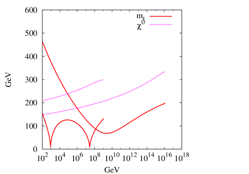
Figure 1: Evolution of the lightest stop and neutralino masses for the $m_{s}\sim 10^{9}$GeV and $m_{s}=m_{GUT}$ scenarios. The tree level stop mass squared is negative for renormalisation mass scales in the range $10^{3}-10^{7}$GeV in the former case, so $\sqrt{|m_{\tilde{t_{1}}}^{2}|}$ is plotted. The boundary condition is $M=350$GeV and $\tan\beta=10$, $\mu$ positive.

Since the MSSM spectrum of these models does not provide a natural candidate for dark matter [31], we have to look for one elsewhere, e.g. in the moduli sector. Also, the models will have to be R-parity violating so that the light stop decays quickly and does not spoil the successful predictions of nucleosynthesis. Another potential difficulty in the cosmological context could be posed by the light bulk moduli for the string scale of order $10^{9}$GeV, as pointed out in Section 2.

The models can still be subjected to other experimental constraints, such as the ones coming from precision measurements of the $b\to s\gamma$ branching ratio and the anomalous magnetic moment of the muon.

The most recent average measurement of the $b\to s\gamma$ branching ratio may be obtained from [32] and is $(3.39\pm 0.30)\times 10^{-4}.$ The theoretical uncertainty in this result is [33] $0.30\times 10^{-4}$; adding the two errors in quadrature, we obtain the $1\sigma$ bound, $BR(b\to s\gamma)=(3.4\pm 0.4)\times 10^{-4}.$

We also impose limits on the new physics contribution to $a_{\mu}=(g_{\mu}-2)/2.$ The experimental value of $a_{\mu}$ is $(11659208\pm 6)\times 10^{-10}$ [34]. The Standard Model computation yields [35, 36] $(11659189\pm 6)\times 10^{-10}$ for the same quantity. This results in the $1\sigma$ bound on the non-SM contribution to $a_{\mu}$, $\delta a_{\mu}=(19\pm 9)\times 10^{10}.$ It is important to note that $\delta a_{\mu}$ usually has the same sign as $\mu$, so $\mu>0$ is preferred by experiment.

We also impose bounds on the Higgs mass obtained by the LEP2 collaborations [37]. The lower bound is $114.4$ GeV at the 95% CL. The error in theoretical predictions is estimated to $3$GeV so we require $m_{h}>111$GeV on the SoftSUSY1.9 prediction.

One can consider a simple modification of this scenario with a raised string scale, by allowing some fine tuning in $W_{0}$. Namely, one can decrease ${\cal{V}}$ while decreasing $W_{0}$, hence increasing $m_{s}$ but also decreasing the amount of SUSY breaking. Let us consider the cases $m_{s}\sim 10^{12}$GeV and $m_{s}\sim 10^{14}$GeV  . In the former case, to make the gauge couplings unify at the string scale, we add $n_{2}=2,n_{E}=3.$ In the $m_{s}\sim 10^{14}$GeV case, we need to add $n_{2}=1,n_{E}=1.$ Interestingly, already in the $m_{s}\sim 10^{12}$GeV case, the LSP becomes a neutralino. We can then apply the hypothesis that the neutralino constitutes all of the cold dark matter relic density. The WMAP [38, 39] constraint on the relic density of dark matter particles (at the $3\sigma$ level) is

$$0.084<\Omega h^{2}<0.138.$$ (10)

However, the $B=-2M$ condition cannot be satisfied for any values of $m_{s},M$ with $\mu>0$ and can only be satisfied for $\mu<0$ for string scales $10^{14}$GeV and above. To see this, one notes that the EWSB conditions

$$\mu^{2} = {{-m_{H_{1}}^{2}\tan^{2}\beta+m_{H_{1}}^{2}}\over{\tan^{2}\beta-1}}-{1\over 2}M_{Z}^{2},$$ (11)

$$\mu B = {1\over 2}\sin 2\beta(m_{H_{1}}^{2}+m_{H_{2}}^{2}+2\mu^{2})$$ (12)

determine the values of $B$ and $\mu$ at the scale $M_{SUSY}=\sqrt{m_{\tilde{t}_{1}}m_{\tilde{t}_{2}}}$ in terms of $\tan\beta$ and the soft breaking masses $m_{H_{1}},m_{H_{2}}.$ One then needs to evolve back to the string scale to check whether the condition $B=-2M$ can be satisfied.

The dependence of the ratio $|B|/(2M)$ on $\tan\beta$ is displayed in Figure 2, for various choices of string scale. Solutions to $B=-2M$ exist only for the low $\tan\beta$ region and $\mu<0.$ However, it can be verified that in this region, the Higgs is too light compared to the LEP2 bound.

Figure 2: Ratio $B({m_{s}})/2M$ for (a) $\mu>0$ and (b) $\mu<0$, $M=350$GeV and $M=1300$GeV.

Therefore we will neglect for the time being the boundary condition $B=-2M$, assuming that the values for the $\mu$ and $B$-terms required for correct electroweak symmetry breaking (EWSB) are generated by some unknown mechanism.

There are then two free parameters, the mass scale $M$ and $\tan\beta.$ The $b\to s\gamma$ branching ratio, $\delta a_{\mu}$ and $\Omega h^{2}$ are computed using the micrOmegas1.3 package [40] interfaced with SoftSUSY1.9 via the SUSY Les Houches Accord [41]. The results are plotted in Figure 3 for $m_{s}\sim 10^{9}$GeV and in Figure 4 for $m_{s}\sim 10^{12}$GeV. Although the dark matter relic density computation is sensitive to the details of the low energy spectrum, the allowed region in the $M-\tan\beta$ plane should not shift significantly when two-loop RGE equations are used instead of one-loop ones. Note that for $\tan\beta$ greater than around 40 one cannot obtain correct EWSB and those values are not included in the graphs. Because the LSP is the stop for $m_{s}\sim 10^{9}$GeV, we do not plot $\Omega h^{2}$ in Figure 3.

Figure 3: Contour plots of $\delta a_{\mu}$ and $BR(b\to s\gamma)$ on $\tan\beta$ and $M$ for (a) $\mu>0$ and (b) $\mu<0$ and $m_{s}\sim 10^{9}$ GeV. $2\sigma$ bounds are used for $\mu>0$ while $3\sigma$ ones are used for $\mu<0.$

Figure 4: Contour plots of $\delta a_{\mu}$, $BR(b\to s\gamma)$ and $\Omega h^{2}$ on $\tan\beta$ and $M$ for (a) $\mu>0$ and (b) $\mu<0$ and $m_{s}\sim 10^{12}$ GeV. $2\sigma$ bounds are used for $\mu>0$ while $3\sigma$ ones are used for $\mu<0.$

MSSM spectra for a few sample points in the parameter space for which both the $\delta a_{\mu}$ and $BR(b\to s\gamma)$ constraints are satisfied are shown in Table 4. The points chosen are denoted by A,B in Figure 3 and C,D in Figure 4. Point C satisfies all the constraints, including the $\chi_{1}^{0}$ cold dark matter hypothesis. The other points satisfy the $BR(b\to s\gamma)$ and $(g-2)_{\mu}$ constraints. In the $m_{s}\sim 10^{12}$GeV, $\mu<0$ case, it is not possible to satisfy the dark matter constraint.

	A	B	C	D
$m_{s}$	$10^{9}$	$10^{9}$	$10^{12}$	$10^{12}$
$\tan\beta$	10	5	6	7
$M$	600	600	370	600
${\rm sgn}\mu$	+	-	+	-
$\tilde{e}_{L},\tilde{\mu}_{L}$	685	684	436	702
$\tilde{e}_{R},\tilde{\mu}_{R}$	633	633	395	637
$\tilde{\tau}_{L}$	681	684	437	699
$\tilde{\tau}_{R}$	618	630	389	630
$\tilde{u}_{1},\tilde{c}_{1}$	973	973	701	1099
$\tilde{u}_{2},\tilde{c}_{2}$	1013	1013	728	1143
$\tilde{t}_{1}$	343	385	237	500
$\tilde{t}_{2}$	885	873	678	973
$\tilde{d}_{1},\tilde{s}_{1}$	968	968	698	1093
$\tilde{d}_{2},\tilde{s}_{2}$	1016	1016	732	1146
$\tilde{b}_{1}$	807	814	593	924
$\tilde{b}_{2}$	949	958	690	1078
$\chi_{1}^{0}$	378	381	201	336
$\chi_{2}^{0}$	543	556	321	544
$\chi_{3}^{0}$	764	802	585	916
$\chi_{4}^{0}$	782	807	601	919
$\chi_{1}^{\pm}$	543	556	321	544
$\chi_{2}^{\pm}$	781	808	600	921
$A_{0},H_{0}$	1008	1065	732	1151
$H^{\pm}$	1012	1067	736	1153
$\tilde{g}$	1014	1014	736	1150
$\tilde{\nu}_{1,2}$	680	680	429	698
$\tilde{\nu}_{3}$	674	679	428	694
$B(b\to s\gamma)/10^{-4}$	$2.8$	$4.4$	$2.9$	$4.3$
$\delta a_{\mu}/10^{-10}$	$3.0$	$-1.6$	$4.2$	$-2.0$
$\Omega h^{2}$	—	—	0.111	2.01

Table 4: Sparticle spectra for the intermediate scale models. All masses are in GeV.

As mentioned before, it is also possible to construct models where gauge unfication does not take place at the string scale. We investigate that possibility for completeness, using the standard MSSM RGEs without any extra matter. In this case, two loop RGEs are used rather than one loop RGEs. The results, however, turn out not to differ significantly from the unification at $m_{s}$ scenario.

4 Matter on D3 branes

Let us now investigate the semi-realistic scenarios that can be constructed assuming the Standard Model lives on a set of D3 branes. For this we have to consider the spectrum in Table 3. Notice that there is a hierarchy between the scalar and the gaugino masses. The difference between the two masses decreases when the string scale is increased. At the GUT scale they tend to be of the same size but apparently too heavy. For any other scale the scalars are much heavier than the gauginos. At an intermediate string scale the scalar masses are of order 1 TeV but the gauginos are too light. At first sight we might conclude that anomaly mediation contribution to the gaugino masses would be dominant but the no-scale nature of our models is such that this contribution is also negligible.

Loop corrections are not large enough to lift the gaugino masses to realistic values. Only for $A$ terms of order $\sim 10^{7}$GeV loop corrections induce gaugino masses of order TeV but at that scale scalar masses are very heavy ($\sim 10^{7}$GeV). We then would have to argue that fine-tuning similar to split supersymmetry is at work to keep the Higgs light.

A second alternative is to consider the case in which the scalar and gaugino masses are of the same order, which in Table 3 corresponds to the GUT scale. Again, the value of $W_{0}$ can be fine tuned to lower the effective masses of scalars and gauginos to the TeV range. We will consider next each of these two scenarios.

4.1 Intermediate Scale Split SUSY

We choose the string scale to be $\sim 10^{13}$GeV, with the scalar masses of order $10^{7}$GeV. One might worry that the gauginos will be extremely heavy as well due to the AMSB contribution. However, it was shown in [42] that in no-scale type models the AMSB contribution to the gaugino mass is vanishing (see the Appendix).

There are two kinds of corrections to this result in our models - firstly, we include perturbative $\alpha^{\prime}$ corrections in the Kähler potential, and secondly, we include nonperturbative contributions to the superpotential $W.$ At tree level, the gaugino masses are set by the size of $F^{S}$, which is induced by nonzero mixing between the dilaton and Kähler moduli once $\alpha^{\prime}$ corrections are included. However, $F^{S}$ is proportional to $1/{\cal{V}}^{2}$ and is very small for large volume. As seen above, the one loop anomaly-induced contribution also vanishes in the no-scale approximation.

In the two Kähler modulus model investigated in [14], we have $\partial_{s}K\sim{1\over{\cal{V}}}$ and $\partial_{b}K\sim{1\over{\cal{V}}^{2/3}}$ with $s,b$ denoting the small and large Kähler moduli, respectively. The nonperturbative contributions to the F-terms are $F_{s}^{np}\sim{1\over{\cal{V}}}$ and $F_{b}^{np}\sim{1\over{\cal{V}}^{4/3}}.$ Therefore, the contributions $K_{i}F^{i}_{np}$ to the gaugino mass in formula (25) in the Appendix scale like $1/{\cal{V}}^{2}.$ Similarly, the contribution to gaugino masses from $F^{S}$ is of the same form. Therefore the anomaly contribution is not as large as would follow from the naive estimate based on just including the superconformal anomaly contribution proportional to $m_{3/2}.$

Hence we arrive at a scenario with the string scale at around $10^{13}$GeV, the scalar masses at $\tilde{m}\sim 10^{7}$GeV and gaugino masses approximately vanishing at the string scale. The first question to be considered is whether it is possible to generate gaugino masses sufficiently large to pass experimental lower bounds through RG evolution to lower scales. To answer this, one must consider the two-loop MSSM RGEs for gaugino masses (as found in [43]):

$${d\over{dt}}M_{a}={2g_{a}^{2}\over{16\pi^{2}}}b_{a}M_{a}+$$

$${2g_{a}^{2}\over{(16\pi^{2})^{2}}}\left(\sum_{b}B_{ab}g_{b}^{2}(M_{a}+M_{b})+\sum_{\alpha=u,d,e}C^{\alpha}_{a}({\rm tr}(Y^{\alpha{\dagger}}h^{\alpha})-M_{a}{\rm tr}(Y^{\alpha^{\dagger}}Y^{\alpha}))\right).$$

The SUSY breaking trilinear scalar couplings $h^{\alpha}$ (defined in terms of the more familiar $A$ notation via $h^{\alpha}_{ij}=A^{\alpha}_{ij}Y^{\alpha}_{ij}$, $Y^{\alpha}$ being the Yukawa couplings) enter the two loop renormalisation; if they are large enough it might be possible to generate sufficient gaugino masses in the running between the string scale and the scalar mass scale.

We will have to assume that the Higgs mass squared is fine-tuned at the scalar mass scale to be negative and of order $-m_{ew}^{2}.$ Given this assumption, below scale $\tilde{m}$, the effective field theory spectrum is that of split supersymmetry [44, 45]: all the SM particles including one light Higgs doublet $H$, together with gauginos $\tilde{B},\tilde{W},\tilde{g}$ and higgsinos $\tilde{H}_{u},\tilde{H}_{d}.$ The Lagrangian consists of kinetic terms and

$$m^{2}H^{\dagger}H-{\lambda\over 2}(H^{\dagger}H)^{2}-\Bigl{(}Y_{ij}^{u}\bar{q}_{j}u_{i}\epsilon H^{*}+Y_{ij}^{d}\bar{q}_{j}d_{i}H+Y_{ij}^{e}\bar{l}_{j}e_{i}H$$

$$+{M_{3}\over 2}\tilde{g}^{A}\tilde{g}^{A}+{M_{2}\over 2}\tilde{W}^{a}\tilde{W}^{a}+{M_{1}\over 2}\tilde{B}\tilde{B}+\mu\tilde{H}_{u}^{T}\epsilon\tilde{H}_{d}$$

$$+{H^{\dagger}\over\sqrt{2}}(\tilde{g}_{u}\sigma^{a}\tilde{W}^{a}+\tilde{g}^{\prime}_{u}\tilde{B})\tilde{H}_{u}+{{H^{T}\epsilon}\over\sqrt{2}}(-\tilde{g}_{d}\sigma^{a}\tilde{W}^{a}+\tilde{g}^{\prime}_{d}\tilde{B})\tilde{H}_{d}+{\rm h.c.}\Bigr{)},$$ (14)

where $\sigma^{a}$ are the Pauli matrices and $\epsilon=i\sigma^{2}.$ Below the scale of the scale of the scalar masses, we use the RGEs of split supersymmetry, listed in the Appendix of [45].

The simplest experimental constraint to impose is the one on the Higgs mass. The Higgs quartic coupling $\lambda$ is matched at the scalar mass scale by the formula

$$\lambda(\tilde{m})={{{g^{2}(\tilde{m})+g^{\prime 2}(\tilde{m})}}\over 4}\cos^{2}{2\beta}.$$ (15)

$g$ and $g^{\prime}$ are the values of the $SU(2)$ and $U(1)_{Y}$ gauge couplings, and the relation between the GUT normalised $g_{1}$ and $g^{\prime}$ is $g_{1}=\sqrt{5/3}g^{\prime}.$ Equation (15) can be obtained by matching the split SUSY Lagrangian (4.1) with the usual SUSY Lagrangian valid above the scalar mass $\tilde{m}.$ It receives finite threshold corrections of order $A^{2}/\tilde{m}^{2}$, but this is negligible in our models. The boundary conditions for $\tilde{g}_{u,d},\tilde{g}^{\prime}_{u,d}$ are similarly given at scale $\tilde{m}$ in terms of $g,g^{\prime}$ and $\tan\beta.$ The values of $g,g^{\prime}$ at the scale $\tilde{m}$ are found by a simple one-loop evolution from their experimentally determined values at $M_{Z}$; after that one evolves $\lambda$ down to $M_{Z}$ using the split SUSY RGEs.

The renormalisation effects on $\lambda$ are large and it is natural to obtain a Higgs significantly heavier than the LEP2 bound. The Higgs mass is estimated as $m_{H}=\sqrt{\lambda}v$ with $v=246.22$GeV. $m_{H}$ ranges from $\sim 142$ GeV to $\sim 163$ GeV depending on the values of $\tan{\beta}$, the top mass and the scalar masses $\tilde{m}.$ The principal dependency is through the value of the top Yukawa, i.e. the top mass. The tree level formula for the Yukawa coupling is $m_{t}^{pole}\sqrt{2}=y_{t}(m_{t})v(m_{t})$, giving $y_{t}=0.99$ for $m_{t}=172.7$ GeV. The dominant one loop corrections to this are [47]

$$m_{t}^{pole}\sqrt{2}=y_{t}(m_{t})v(m_{t})\left(1+{g_{3}^{2}(m_{t})\over{3\pi^{2}}}-{y_{t}^{2}(m_{t})\over{8\pi^{2}}}\right),$$ (16)

giving $y_{t}(m_{t})=0.96.$ We use the 1-loop corrected value for greater accuracy. As can be seen in Figure 5, the Higgs mass is essentially independent of $\tan\beta$ for large values of $\tan\beta.$

Figure 5: The value of the Higgs mass against $\tan\beta$ for $\tilde{m}=10^{6}$GeV and $\tilde{m}=10^{8}$GeV.

Next we study the RGE evolution of gaugino masses and the $\mu$-term. We assume that the gaugino masses at the high scale are close to $0$GeV and that the magnitude of the $\mu$-term is tuned to $100$GeV. The A-terms are taken to be negative and between $10^{4}$ and $10^{7}$ GeV in magnitude. With these initial conditions at the string scale $m_{s}$ we evolve down to the scalar mass scale $\tilde{m}.$ The results for gaugino masses and the $\mu$-term at the scale of $M_{Z}$ are shown in Figure 6. The salient features are a heavy gluino, a slight change in the $\mu$-term, a small increase in $M_{1}$, and a moderate one in $M_{2}.$

Figure 6: Gaugino masses and the $\mu$-term for $\tilde{m}=10^{6},10^{7},10^{8}$GeV. The boundary condition at the string scale is $M_{1}=M_{2}=M_{3}=1$GeV and $\mu=100$GeV.

We have checked that the results are largely insensitive to the choice of gaugino masses at $m_{s}$ in the range $0-10$GeV. We also investigated the effects of modifying the RGE equations above the scale $\tilde{m}$ so that the gauge couplings unify at the string scale of around $10^{13}$GeV. This is achieved by having 2 extra lepton doublets and 3 extra lepton singlets. Again, the results for gaugino masses and the $\mu$ term at scale $M_{Z}$ are largely unaffected.

The next issue to address is that of dark matter in this scenario. As discussed in [45], there are three different possibilities.

The Bino by itself cannot be the dark matter particle, since it is a gauge singlet and only interacts with the Higgs and higgsinos through the terms

$${H^{\dagger}\over\sqrt{2}}\tilde{g}^{\prime}_{u}\tilde{B}\tilde{H}_{u}+{H^{T}\epsilon\over\sqrt{2}}\tilde{g}^{\prime}_{d}\tilde{B}\tilde{H}_{d}+{\rm h.c.}$$ (17)

Therefore not a sufficient number of channels are available for its annihilation and the resulting dark matter density would be too large [45].

The LSP could be a mixture of Bino and higgsino if $M_{1}$ and $\mu$ are comparable in size, with relic density

$$\Omega_{\chi}h^{2}\approx 0.1{{{\mu^{2}}(M_{1}^{2}+\mu^{2})^{2}}\over{m_{\chi}^{4}{\rm TeV}^{2}}}.$$ (18)

We consider the $\tilde{m}=10^{7}$GeV scenario, with $\mu=200$GeV at the string scale. The relic density is computed using formula (18) and its dependence on $\tan\beta$ is shown in Figure 7. Also included is the graph of the relic density for $\tilde{m}=10^{8}$GeV and $\mu=500$GeV at the string scale. It is clear that with appropriately chosen values of $\mu$ and $\tan\beta$ it is possible to obtain an acceptable dark matter relic density. The particle spectrum for $\tilde{m}=10^{7}$GeV, $\mu=200$GeV and $\tan\beta=22$, satisfying the dark matter hypothesis, is shown in Table 5.

Particle	Mass
$\chi_{1}^{0}$	123
$\chi_{2}^{0}$	204
$\chi_{3}^{0}$	240
$\chi_{4}^{0}$	407
$\chi_{1}^{+}$	212
$\chi_{2}^{+}$	383
$\tilde{g}$	1033
$\Omega h^{2}$	0.11

Table 5: Supersymmetric particle spectrum for $\tilde{m}=10^{7}$GeV, $\mu=200$GeV and $\tan\beta=22.$

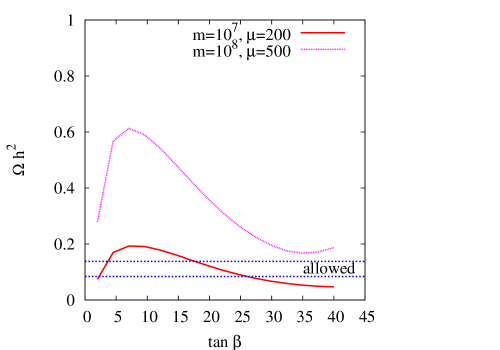
Figure 7: The dark matter relic density $\Omega h^{2}$ in the heavy scalar scenario, for $\tilde{m}=10^{7}$GeV, $\mu=200$GeV and $\tilde{m}=10^{8}$GeV, $\mu=500$GeV.

The second case is that of a heavy higgsino being the LSP. In this case the relic abundance is

$$\Omega_{\tilde{H}}h^{2}=0.09\left(\mu\over{\rm TeV}\right)^{2}.$$ (19)

Scenarios with $\tilde{m}$ slightly above $10^{8}$GeV can realise this possibility, since then the Bino has mass above $700$GeV. With a $\mu$-term chosen to be $1-1.2$TeV at the string scale $m_{s}$, it is possible to obtain the correct relic abundance. For example, with $A=-3\times 10^{6}$GeV and $\tan\beta=40$ we have (at scale $M_{Z}$) $M_{1}\sim 2200$GeV, $M_{2}\sim 5600$GeV, $M_{3}\sim 12000$GeV whereas $\mu=1006$GeV.

The last possibility is that of a Wino LSP and relic abundance

$$\Omega_{\tilde{W}}h^{2}=0.02\left({M_{2}\over{\rm TeV}}\right)^{2}.$$ (20)

However, this cannot be realised in our scenarios, since the Wino is always heavier than the Bino.

4.2 Stringy mSUGRA

We note that the string scale is independent of the flux superpotential parameter $W_{0}$, whereas all the soft terms are directly proportional to it. Therefore we can take $m_{s}\sim 10^{16}$GeV, put all the matter on D3 branes and lower the value of $W_{0}$ to obtain realistic values for the scalar masses and other soft parameters. Note that the gravitino mass will also be lowered in this process, and its size will be roughly just one order of magnitude above the scalar masses. We must be careful for a number of reasons, since lowering $W_{0}$ means lowering the magnitude of supersymmetry breaking in the nonSUSY AdS minimum of [14]. Therefore the D-term contribution to SUSY breaking might become significant compared to the F-term contributions. However, this is not the case since both D and F-terms are proportional to the value of $W_{0}.$

Therefore, we have two parameters to control - $\cal{V}$ and $W_{0}.$ Increasing $\cal{V}$ decreases the string scale, while decreasing $W_{0}$ decreases the soft terms only (since the amount of supersymmetry breaking is reduced). However, the only reasonable scenarios with scalar masses of ${\cal{O}}(1{\rm TeV})$ will arise from the scenario with string scale $10^{16}$GeV and appropriately reduced $W_{0}.$ The string scale cannot be reduced any further, since that would entail increasing ${\cal{V}}$ significantly and the ratio of gaugino to scalar masses would become very small, leading back to the split SUSY scenario.

5 Other possibilities

One could also consider D3 or D7 branes in a warped region, so that the warp factor reduces the scalar masses to a small value. This however also reduces the value of the string scale to a smaller value. The resulting small gap between the scalar mass scale and the string scale makes it difficult to achieve unification at the string scale - one needs a large amount of extra matter. For example, if the string scale is lowered to $10^{6}$ GeV, one needs at least 14 new multiplets, and with the string scale at $10^{4}$GeV, one needs 51. The construction of string models in which this type of scenarios can be realised is open.

6 Conclusions

We have presented three distinctive scenarios of low-energy supersymmetry breaking which were derived from string compactifications. It is very appealing to be able go such a long way - from a string theory compactification with fluxes to computing the spectrum at low energy of specific models. It is also illustrative to see how difficult it is to obtain fully realistic scenarios given the many cosmological and phenomenological constraints.

The three scenarios we studied have several interesting properties and represent a progress in the right direction to close the gap between string theory and low-energy physics. In particular the detailed spectrum of supersymmetric particles was obtained at low-energies for representative examples.

Each of the scenarios has potential problems which illustrate the difficulties that can be expected in general. The generalised fluxed MSSM scenario, despite its interesting features, has to face the cosmological moduli problem which appears at every value of the string scale, as mentioned in the text. We would have to rely on a solution of this problem in order to consider this scenario to be fully realistic. Notice that this potential problem could not have been envisioned in the original discussion of soft supersymmetry breaking induced by fluxes since there was no mechanism to fix the Kähler structure moduli. Also, for scales lower than $10^{12}$GeV the stop is the LSP instead of a neutralino. Barring these problems we found that the parameter space is greatly reduced by the standard phenomenological constraints. The case $\mu>0$ is not compatible with the boundary condition for the $B$ term, while for $\mu<0,m_{s}<10^{16}$GeV only low $\tan\beta$ solutions exist and the Higgs mass is below the LEP2 bound. This problem may be alleviated by relaxing the $B$ term boundary condition, e.g. by considering the Higgs coming from D3-D7 strings. Our lack of control of the Kähler potential for these fields does not allow us to make a concrete statement about this possibility.

The intermediate scale split supersymmetry scenario needs the usual fine tuning in order to keep the Higgs light. Again the D3-D7 particles could alleviate this problem if their masses were under control. Furthermore, despite sharing with the split supersymmetry scenario the property that the scalars are hierarchically heavier than the gauginos, it has to be pointed out that in our scenario the string scale is intermediate and therefore we do not expect the standard MSSM gauge coupling unification to work.

The stringy mSUGRA scenario requires a tuning of the flux superpotential in order to achieve a GUT string scale. This tuning however may be argued to be less severe than the tuning of the split supersymmetry that needs to be made at the spectrum level, although both rely on the existence of many flux vacua. Notice that in the stringy mSUGRA scenario, without knowing any relationship among the relative coefficients, we can only estimate the order of magnitude of the soft breaking terms.

It is fair to say also that each of the phenomenological constraints we have used may be relaxed and the parameter space of realistic models can be substantially enhanced. For example, non-universal flavour structure in the soft SUSY breaking terms can cancel the supersymmetric contribution to BR$(b\rightarrow s\gamma)$. Also, evidence for a non-Standard Model component of $(g-2)_{\mu}$ is controversial and may turn out to not be relevant. Similarly, dark matter could all reside in the hidden sector and the LSP could be unstable.

It is interesting to compare our results with the phenomenology of KKLT-type scenarios. The essential difference is that the large volume minima we found are non-supersymmetric even before the lifting term is added. In KKLT scenarios, supersymmetry is restored after fixing the Kähler moduli, so it is precisely the anti D3 brane term which is responsible for supersymmetry breaking. Of course, the uplift gives non-zero values to F-terms as well, but these will be parametrised in terms of the uplift potential. In fact it turns out [8, 9] that they are significantly suppressed with respect to the no-scale model values. This implies that, for example, the moduli mediated contribution to the D7 scalar masses is suppressed with respect to $m_{3/2}$ and will generically compete with the AMSB contribution. The same is true for gaugino masses, where it turns out that it is possible to obtain a ‘mirage unification’ at the intermediate or even TeV scale by combining the two contributions [10, 11, 12]. There were no realistic scenarios for D3 soft terms in that scenario.

Finally, it is worth pointing out that what we have analysed here are general scenarios assuming that the Standard Model is on D3 or D7 branes. In order to be more concrete it would be desirable to carry out this kind of analysis on explicit D-brane models, taking into account potential matter and gauge fields beyond the MSSM, etc. There are clearly many things to be done in this direction. Explicit model building may become more focused after data from the Large Hadron Collider (LHC) arrives.

Appendix A Appendix: Gaugino Masses in No-Scale Models

Let us consider the general formula for the gaugino mass in models with both moduli and anomaly mediated SUSY breaking, as derived in [42]:

$$m_{G}=-{g^{2}\over{16\pi^{2}}}\left((3T_{G}-T_{R})m_{3/2}+(T_{G}-T_{R})K_{i}F^{i}+{2T_{R}\over d_{R}}(\log\det K|_{R}^{{}^{\prime\prime}})_{,i}F^{i}\right)$$ (21)

Here $T_{G}$ is the Dynkin index for the adjoint representation, $3T_{G}-T_{R}$ is the one-loop gauge beta function coefficient and $T_{R}$ is the Dynkin index associated with the representation $R$ of dimension $d_{R}$, equal to $1/2$ for the $SU(N)$ fundamental; a sum over all the matter representations $R$ is understood in each term with the $R$ subindex. $K$ is the Kähler potential, $K^{\prime\prime}|_{R}$ its second derivatives with respect to matter fields projected onto the corresponding representation of $G$, and the F-terms are defined as

$$F^{i}=-e^{K/2}K^{i\bar{\jmath}}\,\overline{D_{j}W},$$ (22)

with $W$ the superpotential. The first term in equation (21) is the usual super-Weyl anomaly induced term present in any supergravity theory. The second and third terms arise from Kähler and sigma-model anomalies.

For simplicity let us consider the case of a single Kähler modulus model. Let us assume that the Kähler potential is of the no-scale form,

$$K=-3\log\left(T+T^{*}-{1\over 3}\phi\phi^{*}\right)$$ (23)

where $\phi$ is the matter field. Taking derivatives with respect to matter fields, one gets the result for a particular representation $R$

$${1\over{d_{R}}}\log\det K|_{R}^{{}^{\prime\prime}}={1\over 3}K,$$ (24)

assuming that the vevs of visible matter vanish. Hence from formula (21) we get

$$m_{G} = -{g^{2}\over{16\pi^{2}}}\left((3T_{G}-T_{R})m_{3/2}+(T_{G}-T_{R})K_{i}F^{i}+{2\over 3}T_{R}K_{i}F^{i}\right)$$ (25)

$$= -{g^{2}\over{48\pi^{2}}}(3T_{G}-T_{R})(3m_{3/2}+K_{i}F^{i}).$$ (26)

In no-scale models SUSY breaking corresponds to nonzero values of the auxiliary field corresponding to $T.$ The gravitino mass is equal to

$$m_{3/2}=e^{K/2}W.$$ (27)

Also

$$F^{T}=-e^{K/2}K^{T\bar{T}}D_{T}W=-e^{K/2}{(T+T^{*})^{2}\over 3}(\partial_{T}K)W=e^{K/2}(T+T^{*})W.$$ (28)

assuming that $T$ is absent from the superpotential. Therefore we have

$$K_{T}F^{T}+3m_{3/2}=-3e^{K/2}W+3e^{K/2}W=0.$$ (29)

It can easily be checked that this result generalises to the $n$-Kähler modulus case, due to the no-scale property $K^{i{\bar{\jmath}}}\partial_{i}K\partial_{\bar{\jmath}}K=3$ with $i,j$ ranging over all Kähler moduli. It follows from equation (25) that the AMSB contribution to gaugino masses is vanishing.

References

- [1] D. J. H. Chung, L. L. Everett, G. L. Kane, S. F. King, J. D. Lykken and L. T. Wang, “The soft supersymmetry-breaking Lagrangian: Theory and applications,” Phys. Rept. 407, 1 (2005) [arXiv:hep-ph/0312378].
- [2] B. C. Allanach et al., “The Snowmass points and slopes: Benchmarks for SUSY searches,” in Proc. of the APS/DPF/DPB Summer Study on the Future of Particle Physics (Snowmass 2001) ed. N. Graf, Eur. Phys. J. C 25, 113 (2002) [eConf C010630, P125 (2001)] [arXiv:hep-ph/0202233].
- [3] M. Battaglia et al., “Proposed post-LEP benchmarks for supersymmetry,” Eur. Phys. J. C 22, 535 (2001) [arXiv:hep-ph/0106204].
- [4] A. Brignole, L. E. Ibanez and C. Munoz, “Soft supersymmetry-breaking terms from supergravity and superstring models,” arXiv:hep-ph/9707209.
- [5] S. Kachru, R. Kallosh, A. Linde and S. P. Trivedi, “De Sitter vacua in string theory,” Phys. Rev. D 68, 046005 (2003) [arXiv:hep-th/0301240].
- [6] M. Grana, “MSSM parameters from supergravity backgrounds,” Phys. Rev. D 67, 066006 (2003) [arXiv:hep-th/0209200]; P. G. Camara, L. E. Ibanez and A. M. Uranga, “Flux-induced SUSY-breaking soft terms,” Nucl. Phys. B 689, 195 (2004) [arXiv:hep-th/0311241]; M. Grana, T. W. Grimm, H. Jockers and J. Louis, “Soft supersymmetry breaking in Calabi-Yau orientifolds with D-branes and fluxes,” Nucl. Phys. B 690, 21 (2004) [arXiv:hep-th/0312232]; D. Lust, S. Reffert and S. Stieberger, “Flux-induced soft supersymmetry breaking in chiral type IIb orientifolds with D3/D7-branes,” Nucl. Phys. B 706, 3 (2005) [arXiv:hep-th/0406092]; P. G. Camara, L. E. Ibanez and A. M. Uranga, “Flux-induced SUSY-breaking soft terms on D7-D3 brane systems,” Nucl. Phys. B 708, 268 (2005) [arXiv:hep-th/0408036]. A. Font and L. E. Ibanez, “SUSY-breaking soft terms in a MSSM magnetized D7-brane model,” JHEP 0503, 040 (2005) [arXiv:hep-th/0412150].
- [7] B. C. Allanach, A. Brignole and L. E. Ibanez, “Phenomenology of a fluxed MSSM,” JHEP 0505, 030 (2005) [arXiv:hep-ph/0502151].
- [8] K. Choi, A. Falkowski, H. P. Nilles and M. Olechowski, “Soft supersymmetry breaking in KKLT flux compactification,” Nucl. Phys. B 718, 113 (2005) [arXiv:hep-th/0503216].
- [9] A. Falkowski, O. Lebedev and Y. Mambrini, “SUSY phenomenology of KKLT flux compactifications,” arXiv:hep-ph/0507110.
- [10] K. Choi, K. S. Jeong and K. i. Okumura, “Phenomenology of mixed modulus-anomaly mediation in fluxed string compactifications and brane models,” JHEP 0509, 039 (2005) [arXiv:hep-ph/0504037].
- [11] M. Endo, M. Yamaguchi and K. Yoshioka, “A bottom-up approach to moduli dynamics in heavy gravitino scenario: Superpotential, soft terms and sparticle mass spectrum,” Phys. Rev. D 72, 015004 (2005) [arXiv:hep-ph/0504036].
- [12] O. Lebedev, H. P. Nilles and M. Ratz, “A note on fine-tuning in mirage mediation,” arXiv:hep-ph/0511320.
- [13] V. Balasubramanian, P. Berglund, J. P. Conlon and F. Quevedo, “Systematics of moduli stabilisation in Calabi-Yau flux compactifications,” JHEP 0503, 007 (2005) [arXiv:hep-th/0502058].
- [14] J. P. Conlon, F. Quevedo and K. Suruliz, “Large-volume flux compactifications: Moduli spectrum and D3/D7 soft JHEP 0508, 007 (2005) [arXiv:hep-th/0505076].
- [15] L. E. Ibanez, “The fluxed MSSM,” Phys. Rev. D 71, 055005 (2005) [arXiv:hep-ph/0408064].
- [16] C. P. Burgess, R. Kallosh and F. Quevedo, “de Sitter string vacua from supersymmetric D-terms,” JHEP 0310 (2003) 056 [arXiv:hep-th/0309187]; G. Villadoro and F. Zwirner, “de Sitter vacua via consistent D-terms,” arXiv:hep-th/0508167.
- [17] A. Saltman and E. Silverstein, “The scaling of the no-scale potential and de Sitter model building,” JHEP 0411 (2004) 066 [arXiv:hep-th/0402135].
- [18] T. Banks, D. B. Kaplan and A. E. Nelson, “Cosmological implications of dynamical supersymmetry breaking,” Phys. Rev. D 49, 779 (1994) [arXiv:hep-ph/9308292].
- [19] B. de Carlos, J. A. Casas, F. Quevedo and E. Roulet, “Model independent properties and cosmological implications of the dilaton and moduli sectors of 4-d strings,” Phys. Lett. B 318, 447 (1993) [arXiv:hep-ph/9308325].
- [20] G. D. Coughlan, W. Fischler, E. W. Kolb, S. Raby and G. G. Ross, “Cosmological Problems For The Polonyi Potential,” Phys. Lett. B 131, 59 (1983).
- [21] G. Aldazabal, L. E. Ibanez, F. Quevedo and A. M. Uranga, “D-branes at singularities: A bottom-up approach to the string embedding of the standard model,” JHEP 0008, 002 (2000) [arXiv:hep-th/0005067]; G. Aldazabal, L. E. Ibanez and F. Quevedo, “Standard-like models with broken supersymmetry from type I string vacua,” JHEP 0001 (2000) 031 [arXiv:hep-th/9909172]; “A D-brane alternative to the MSSM,” JHEP 0002 (2000) 015 [arXiv:hep-ph/0001083].
- [22] J. F. G. Cascales, M. P. Garcia del Moral, F. Quevedo and A. M. Uranga, “Realistic D-brane models on warped throats: Fluxes, hierarchies and moduli stabilization,” JHEP 0402, 031 (2004) [arXiv:hep-th/0312051].
- [23] D. Berenstein, V. Jejjala and R. G. Leigh, “The standard model on a D-brane,” Phys. Rev. Lett. 88, 071602 (2002) [arXiv:hep-ph/0105042].
- [24] H. Verlinde and M. Wijnholt, “Building the standard model on a D3-brane,” arXiv:hep-th/0508089.
- [25] J. F. G. Cascales, F. Saad and A. M. Uranga, “Holographic dual of the standard model on the throat,” arXiv:hep-th/0503079.
- [26] B. C. Allanach and S. F. King, “String unification, spaghetti diagrams and infra-red fixed points,” Nucl. Phys. B 507, 91 (1997) [arXiv:hep-ph/9703293].
- [27] B. C. Allanach, “SOFTSUSY: A C++ program for calculating supersymmetric spectra,” Comput. Phys. Commun. 143, 305 (2002) [arXiv:hep-ph/0104145].
- [28] [CDF Collaboration], “Combination of CDF and D0 results on the top-quark mass,” arXiv:hep-ex/0507091.
- [29] S. Eidelman et al. [Particle Data Group], “Review of particle physics,” Phys. Lett. B 592, 1 (2004).
- [30] J. A. Casas, A. Lleyda and C. Munoz, “Strong constraints on the parameter space of the MSSM from charge and color breaking minima,” Nucl. Phys. B 471, 3 (1996) [arXiv:hep-ph/9507294].
- [31] P. F. Smith, J. R. J. Bennett, G. J. Homer, J. D. Lewin, H. E. Walford and W. A. Smith, “A Search For Anomalous Hydrogen In Enriched D-2 O, Using A Time-Of-Flight Spectrometer,” Nucl. Phys. B 206, 333 (1982).
-
[32]
Heavy Flavour Averaging Group Collaboration.
http://www.slac.stanford.edu/xorg/hfag - [33] P. Gambino, U. Haisch and M. Misiak, “Determining the sign of the b s gamma amplitude,” Phys. Rev. Lett. 94, 061803 (2005) [arXiv:hep-ph/0410155].
- [34] G. W. Bennett et al. [Muon g-2 Collaboration], Phys. Rev. Lett. 92, 161802 (2004) [arXiv:hep-ex/0401008].
- [35] M. Passera, “The standard model prediction of the muon anomalous magnetic moment,” J. Phys. G 31, R75 (2005) [arXiv:hep-ph/0411168].
- [36] J. F. de Troconiz and F. J. Yndurain, “The hadronic contributions to the anomalous magnetic moment of the muon,” Phys. Rev. D 71, 073008 (2005) [arXiv:hep-ph/0402285].
- [37] R. Barate et al. [ALEPH Collaboration], “Search for the standard model Higgs boson at LEP,” Phys. Lett. B 565, 61 (2003) [arXiv:hep-ex/0306033].
- [38] D. N. Spergel et al. [WMAP Collaboration], “First Year Wilkinson Microwave Anisotropy Probe (WMAP) Observations: Astrophys. J. Suppl. 148, 175 (2003) [arXiv:astro-ph/0302209].
- [39] C. L. Bennett et al., “First Year Wilkinson Microwave Anisotropy Probe (WMAP) Observations: Astrophys. J. Suppl. 148, 1 (2003) [arXiv:astro-ph/0302207].
- [40] G. Belanger, F. Boudjema, A. Pukhov and A. Semenov, “MicrOMEGAs: Version 1.3,” arXiv:hep-ph/0405253.
- [41] P. Skands et al., “SUSY Les Houches accord: Interfacing SUSY spectrum calculators, decay packages, and event generators,” JHEP 0407, 036 (2004) [arXiv:hep-ph/0311123].
- [42] J. A. Bagger, T. Moroi and E. Poppitz, “Anomaly mediation in supergravity theories,” JHEP 0004, 009 (2000) [arXiv:hep-th/9911029].
- [43] S. P. Martin and M. T. Vaughn, “Two loop renormalization group equations for soft supersymmetry breaking Phys. Rev. D 50, 2282 (1994) [arXiv:hep-ph/9311340].
- [44] N. Arkani-Hamed and S. Dimopoulos, “Supersymmetric unification without low energy supersymmetry and signatures JHEP 0506, 073 (2005) [arXiv:hep-th/0405159].
- [45] G. F. Giudice and A. Romanino, “Split supersymmetry,” Nucl. Phys. B 699, 65 (2004) [Erratum-ibid. B 706, 65 (2005)] [arXiv:hep-ph/0406088].
- [46] A. Arvanitaki, C. Davis, P. W. Graham and J. G. Wacker, “One loop predictions of the finely tuned SSM,” Phys. Rev. D 70, 117703 (2004) [arXiv:hep-ph/0406034].
- [47] H. E. Haber, R. Hempfling and A. H. Hoang, “Approximating the radiatively corrected Higgs mass in the minimal supersymmetric model,” Z. Phys. C 75, 539 (1997) [arXiv:hep-ph/9609331].