Gluon propagation
inside a high-energy nucleus

Abstract

We show that, in the light-cone gauge, it is possible to derive in a very simple way the solution of the classical Yang-Mills equations for the collision between a nucleus and a proton. One important step of the calculation is the derivation of a formula that describes the propagation of a gluon in the background color field of the nucleus. This allows us to calculate observables in pA collisions in a more straightforward fashion than already proposed. We discuss also the comparison between light-cone gauge and covariant gauge in view of further investigations involving higher order corrections.

1. Service de Physique Théorique
   CEA/DSM/Saclay, Bât. 774
   91191, Gif-sur-Yvette Cedex, France

2. Laboratoire de Physique Théorique
   Université Paris Sud, Bât. 210
   91405, Orsay cedex

Preprint SPhT-T05/194

LPT-Orsay 05-83

1 Introduction

The study of semi-hard particle production in high energy hadronic interaction is dominated by interactions between partons having a small fraction $x$ of the longitudinal momentum of the colliding nucleons. Since the phase-space density of such partons in the nucleon wave function is large, one expects that the physics of parton saturation [1, 2, 3] plays an important role in such studies. This saturation generally has the effect of reducing the number of produced particles compared to what one would have predicted on the basis of pQDC calculation with parton densities that depend on $x$ according to the linear BFKL [4, 5] evolution equation.

It was proposed by McLerran and Venugopalan [6, 7, 8] that one could take advantage of this large phase-space density in order to describe the small $x$ partons by a classical color field rather than as particles. More precisely, the McLerran-Venugopalan (MV) model proposes a dual description, in which the small $x$ partons are described as a classical field and the large $x$ partons act as color sources for the classical field. In their original model, they had in mind a large nucleus, for which there would be a large number of large $x$ partons (at least $3A$ where $A$ is the atomic number of the nucleus, from just counting the valence quarks) and therefore they would produce a strong color source. This meant that one has to solve the full classical Yang-Mills equations in order to find the classical field. But that procedure, on the other hand, would properly incorporate the recombination interactions that are responsible for gluon saturation. In the MV model, the large $x$ color sources are described by a statistical distribution, which they argued could be taken to be a gaussian for a large nucleus at moderately small $x$ (see also [9] for a more modern perspective on that).

Since then, this model has evolved into a full fledged effective theory, the so-called “Color Glass Condensate” (CGC) [10, 11, 12]. It was soon recognized that the separation between what one calls large $x$ and small $x$, inherent to the dual description of the MV model, is somewhat arbitrary, and that the gaussian nature of the distribution of sources would not survive upon changes of this separation scale. This arbitrariness has been exploited to derive a renormalization group equation, the so-called JIMWLK equation [13, 14, 15, 16, 17, 18, 19, 10, 11, 12], that describes how the statistical distribution of color sources changes as one moves the boundary between large $x$ and small $x$. This functional evolution equation can also be expressed as an infinite hierarchy of evolution equations for correlators [20], and has a quite useful (and tremendously simpler) large $N_{c}$ mean-field approximation [21], known as the Balitsky-Kovchegov equation.

In high energy hadronic collisions, gluon production is dominated by the classical field approximation, and calculating it requires to solve the classical Yang-Mills equations for two color sources moving at the speed of light in opposite directions. This is a problem that has been solved numerically in [22, 23, 24, 25, 26] for the boost-invariant case, and the stability of this solution against rapidity dependent perturbations has been investigated in [27, 28]. In terms of analytical solutions, much less is known. The only situation for which gluon production has been calculated analytically is the case where one of the two sources is weak and can thus be treated at lowest order (this situation is often referred to as “proton-nucleus” collisions in the literature, but it can also be encountered at forward rapidities in the collision of two identical objects). This was done in a number of approaches [29, 31, 32, 33]. The last two references provide the solution of Yang-Mills equation in this asymmetrical situation, in the Schwinger gauge ($x^{+}A^{-}+x^{-}A^{+}=0$) and Lorenz gauge ($\partial_{\mu}A^{\mu}=0$) respectively. More recently, Balitsky has proposed an expansion in commutators of Wilson lines, where at each order one treats the two projectiles symmetrically [34].

Although the solution in the Lorenz gauge was fairly compact, it turned out that it displayed some oddities like the appearance of a Wilson line containing the coupling constant $g/2$ instead of $g$ (this of course disappeared at later stages from physical quantities). When applied to the production of quark-antiquark production in [35], it also led to a contribution in which the vertex producing the $q\bar{q}$ pair was located inside the nucleus, which is quite counter-intuitive.

In this paper, we derive the solution of the Yang-Mills equations in the light-cone gauge $A^{+}=0$ (with the nucleus moving in the negative $z$ direction), and we find a much simpler solution (not only the solution is simpler, but it is also much easier to obtain). In particular, the solution in the $A^{+}=0$ gauge presents none of the odd features encountered in the Lorenz gauge. Our central result, derived in section 2, is in fact a formula that tells how a color field propagates on top of the gauge field of the nucleus. The eqs. (12) in fact contain all the information which is needed in order to derive the solution of Yang-Mills equations and compute gluon production, which we perform as a verification in section 3. Beyond the study of “proton-nucleus” collisions themselves, eqs. (12) are an important building block for calculating higher order corrections in the weak source to the solution of Yang-Mills equations. And to a large extent, the complexity of this object finds its way into the solution of Yang-Mills equations. Therefore, it is important to determine this object, and to find a gauge in which it is particularly simple. For the sake of comparison, we derive in appendix A the analogue of eqs. (12) for the Lorenz gauge, and they are much more complicated, as one expects.

2 Gluon propagation in a nucleus

We assume that the nucleus is moving with a velocity very close to the speed of light, in the negative $z$ direction. Thus, it can be described by the following density of color sources:

$$\delta(x^{+})\rho_{a}({\boldsymbol{x}}_{\perp})\;.$$ (1)

Some intermediate calculations may require to regularize the delta function by giving it a small width. When this is necessary, we replace $\delta(x^{+})$ by $\delta_{\epsilon}(x^{+})$, where $\delta_{\epsilon}(x^{+})$ is a positive definite function normalized by $\int_{-\infty}^{+\infty}dx^{+}\;\delta_{\epsilon}(x^{+})=1$ and whose support is $[0,\epsilon]$.

In this paper, we address the following question: knowing the gauge fields at $x^{+}=0$, what are the gauge fields at $x^{+}=\epsilon$, i.e. after having propagated through the nucleus? Finding the gluon propagator inside the nucleus amounts to solving this problem to linear order in the incoming gauge fields. In practice, we add to the gauge field $A^{\mu}_{0}$ of the nucleus a small perturbation $A^{\mu}_{1}$,

$$A^{\mu}=A_{0}^{\mu}+A_{1}^{\mu}\;,$$ (2)

and we wish to find a linear relationship for this perturbation before and after the region where the nucleus lives, such as (see figure 1) :

$$A^{\mu}_{1}(x^{+}=\epsilon)=M^{\mu}{}_{\nu}\;A_{1}^{\nu}(x^{+}=0)\;.$$ (3)

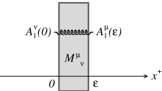
Figure 1: Gluon passing through a nucleus. The region shaded in gray is the region where the color source representing the nucleus is non-zero.

We work in the light-cone gauge $A^{+}=0$. The covariant conservation of the color current reads:

$$\partial^{+}J^{-}+[D^{-},J^{+}]-[D^{i},J^{i}]=0\;.$$ (4)

This equation can be solved by

$$J^{+}=J^{i}=0\;,$$

$$\partial^{+}J^{-}=0\;.$$ (5)

The first equation is allowed because all the color charges in our problem are moving in the negative $z$ direction. The second equation means that the color current $J^{-}$ associated to the nucleus is not affected by the incoming field, and therefore this current $J^{-}$ can be “hidden” once for all in the gauge field $A^{\mu}_{0}$ of the nucleus.

The Yang-Mills equations in this gauge read

$$\partial^{+}(\partial_{\mu}A^{\mu})+ig[A^{i},\partial^{+}A^{i}]=0$$

$$[D^{-},\partial^{+}A^{-}]-[D^{i},F^{i-}]=J^{-}$$

$$\partial^{+}F^{-i}+[D^{-},\partial^{+}A^{i}]-[D^{j},F^{ji}]=0\;.$$ (6)

One can see that the first of these equations does not contain any time derivative ($\partial^{-}$). Therefore, it can be seen as a constraint that relates the various field components at the same time.

The gauge field of the nucleus alone is found by considering only the order zero in $A_{1}^{\mu}$ in the above equations. One can readily check that the following is a solution:

$$A_{0}^{i}=0\quad,\quad A_{0}^{-}=-\frac{1}{{\boldsymbol{\partial}}_{\perp}^{2}}J^{-}=-g\delta(x^{+})\frac{1}{{\boldsymbol{\partial}}_{\perp}^{2}}\rho(x_{\perp})\;.$$ (7)

In order to find the the linear relationship between the perturbation $A_{1}^{\mu}$ before and after the region where the color sources of the nucleus live, we must linearize the Yang-Mills equations in $A_{1}^{\mu}$. One obtains

$$\partial^{+}A_{1}^{-}-\partial^{i}A_{1}^{i}=0$$

$$\square A_{1}^{i}-2ig[A_{0}^{-},\partial^{+}A^{i}]=0$$

$$\square A_{1}^{-}-2ig[A_{0}^{-},\partial^{+}A_{1}^{-}]=2ig[\partial^{i}A_{0}^{-},A_{1}^{i}]=2ig(\partial^{i}A_{0}^{-}\cdot T)A_{1}^{i}\;.$$ (8)

The method for solving the second and third equations was explained in [33]. The solution of the second equation inside the nucleus, i.e. for $x^{+}\in[0,\epsilon]$, reads:

$$A_{1}^{i}(x^{+},x^{-},{\boldsymbol{x}}_{\perp})=U(x^{+},0,{\boldsymbol{x}}_{\perp})A_{1}^{i}(0,x^{-},{\boldsymbol{x}}_{\perp})\;,$$ (9)

where $U$ is a Wilson line in the adjoint representation of the gauge group:

$$U(x^{+},0,{\boldsymbol{x}}_{\perp})\equiv{\cal T}_{+}\,\exp\left[ig\int_{0}^{x^{+}}dz^{+}\;A_{0a}^{-}(z^{+},{\boldsymbol{x}}_{\perp})T^{a}\right]\;.$$ (10)

At this point, we could find $A_{1}^{-}$ simply by solving the constraint equation. But as a verification, it is interesting to solve explicitly the third equation for $A_{1}^{-}$, and at the end to verify that the fields $A_{1}^{i}$ and $A_{1}^{-}$ do obey the constraint. The third equation leads to

$$A_{1}^{-}(x^{+},x^{-},{\boldsymbol{x}}_{\perp})=U(x^{+},0,{\boldsymbol{x}}_{\perp})A_{1}^{-}(0,x^{-},{\boldsymbol{x}}_{\perp})$$

$$+ig\int_{0}^{x^{+}}\!\!\!\!dz^{+}U(x^{+},z^{+},{\boldsymbol{x}}_{\perp})(\partial^{i}A_{0}^{-}(z^{+},{\boldsymbol{x}}_{\perp})\cdot T)U(z^{+},0,{\boldsymbol{x}}_{\perp})\frac{1}{\partial^{+}}A_{1}^{i}(0,x^{-},{\boldsymbol{x}}_{\perp})$$

$$=U(x^{+},0,{\boldsymbol{x}}_{\perp})A_{1}^{-}(0,x^{-},{\boldsymbol{x}}_{\perp})+(\partial^{i}U(x^{+},0,{\boldsymbol{x}}_{\perp}))\frac{1}{\partial^{+}}A_{1}^{i}(0,x^{-},{\boldsymbol{x}}_{\perp})\;.$$ (11)

It is trivial to verify that the constraint that relates $A_{1}^{-}$ to $A_{1}^{i}$ would have given the same answer.

Therefore, if we denote $U\equiv U(\epsilon,0,{\boldsymbol{x}}_{\perp})$ and if we don’t write explicitly the $x^{-}$ and ${\boldsymbol{x}}_{\perp}$ dependence, we have the following relations:

$$A_{1}^{+}(\epsilon)=0\;,$$

$$A_{1}^{i}(\epsilon)=UA_{1}^{i}(0)\;,$$

$$A_{1}^{-}(\epsilon)=UA_{1}^{-}(0)+(\partial^{i}U)\frac{1}{\partial^{+}}A_{1}^{i}(0)\;.$$ (12)

These equations are the light-cone gauge expression of the linear relation we were looking for. Analogous relations will be derived for the Lorenz gauge in the appendix A.

3 Gluon production in pA collisions

3.1 Gauge field

¿From this linear relation, it is easy to calculate the gauge field that describes proton-nucleus collisions. In this case, the incoming field $A_{1}^{\mu}$ is the field produced by the current associated to the proton

$$J^{+}=g\delta(x^{-})\rho_{p}({\boldsymbol{x}}_{\perp})\;.$$ (13)

For $x^{+}\leq 0$, i.e. before the collision with the nucleus, the current $J^{+}$ remains constant, and we simply have, to linear order in the proton source $\rho_{p}$

$$A_{1}^{+}=A_{1}^{-}=0\;,$$

$$\square A_{1}^{i}=-\theta(x^{-})\partial^{i}\rho_{p}({\boldsymbol{x}}_{\perp})\;.$$ (14)

Solving the latter equation gives the following field at $x^{+}=0$ :

$$A_{1}^{+}(0)=A_{1}^{-}(0)=0\quad,\quad A_{1}^{i}(0)=\theta(x^{-})\frac{\partial^{i}}{{\boldsymbol{\partial}}_{\perp}^{2}}\rho_{p}({\boldsymbol{x}}_{\perp})\;.$$ (15)

The next step is to use the eqs. (12) in order to find the gauge field $A_{1}^{\mu}$ immediately after the collision with the nucleus, i.e. at $x^{+}=\epsilon$,

$$A_{1}^{+}(\epsilon)=0\;,$$

$$A_{1}^{i}(\epsilon)=U\theta(x^{-})\frac{\partial^{i}}{{\boldsymbol{\partial}}_{\perp}^{2}}\rho_{p}({\boldsymbol{x}}_{\perp})\;,$$

$$A_{1}^{-}(\epsilon)=(\partial^{i}U)\frac{1}{\partial^{+}}\theta(x^{-})\frac{\partial^{i}}{{\boldsymbol{\partial}}_{\perp}^{2}}\rho_{p}({\boldsymbol{x}}_{\perp})\;.$$ (16)

The final step is to find the gauge field for $x^{+}>\epsilon$. The equation that governs the evolution of $A_{1}^{i}$ is

$$\square A_{1}^{i}-2ig[A_{0}^{-},\partial^{+}A_{1}^{i}]=-\frac{\partial^{i}}{\partial^{+}}J^{+}\;,$$ (17)

and the current $J^{+}$ at $x^{+}>\epsilon$ is modified by color precession in the nuclear field $A_{0}^{-}$:

$$J^{+}(x^{+}>\epsilon)=U\delta(x^{-})\rho_{p}({\boldsymbol{x}}_{\perp})\;.$$ (18)

This is a direct consequence of current conservation $D^{-}J^{+}=0$. We must solve eq. (17) with an initial condition at $x^{+}=\epsilon$ given by eq. (16). Using the techniques of [33], we obtain

$$A_{1}^{i}(x)=\int_{y^{+}=\epsilon}dy^{-}d^{2}{\boldsymbol{y}}_{\perp}\;G_{{}_{R}}^{0}(x,y)2\partial_{y}^{+}U({\boldsymbol{y}}_{\perp})\theta(y^{-})\frac{\partial_{y}^{i}}{{\boldsymbol{\partial}}_{{\boldsymbol{y}}_{\perp}}^{2}}\rho_{p}({\boldsymbol{y}}_{\perp})$$

$$\quad+\int_{y^{+}>\epsilon}d^{4}y\;G_{{}_{R}}^{0}(x,y)\theta(y^{-})\partial_{y}^{i}(U({\boldsymbol{y}}_{\perp})\rho_{p}({\boldsymbol{y}}_{\perp}))\;,$$ (19)

where $G_{{}_{R}}^{0}(x,y)$ is the free retarded propagator obeying $\square_{x}G_{{}_{R}}^{0}(x,y)=\delta(x-y)$. The two terms in this solution are illustrated in figure 2.

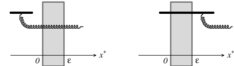
Figure 2: The two contributions to gluon production in pA collisions. Left: the proton source emits the gluon before the collision with the nucleus. Right: the proton source goes through the nucleus before emitting the gluon. The thick solid line represents the proton color current.

3.2 Gluon production

The amplitude for the production of a gluon of momentum $p$ and polarization $\lambda$ is given by the Fourier transform of the amputated gauge field, contracted in the relevant polarization vector,

$${\cal M}_{\lambda}(p)=\int d^{4}x\;e^{ip\cdot x}\square A_{1}^{\mu}(x)\epsilon^{(\lambda)}_{\mu}({\boldsymbol{p}})\;.$$ (20)

In light-cone gauge, the sum over the physical polarizations reads

$$\sum_{\lambda}\epsilon^{(\lambda)}_{i}({\boldsymbol{p}})\epsilon^{(\lambda)*}_{j}({\boldsymbol{p}})=-g_{ij}\;,$$ (21)

and for this reason we need only the transverse components of the gauge field when calculating gluon production. Note that since the Dalembertian $\square A_{1}^{i}(x)$ is bounded inside the nucleus, the region $0<x^{+}<\epsilon$ does not contribute in the limit $\epsilon\to 0$. Therefore, we can take $\epsilon\to 0$ and disregard the interior of the nucleus when we calculate the amplitude. We first obtain:

$$\square A_{1}^{i}(x) = 2\delta(x^{+})\delta(x^{-})(U-1)\frac{\partial^{i}}{{\boldsymbol{\partial}}^{2}_{\perp}}\rho_{p}({\boldsymbol{x}}_{\perp})$$ (22)

$$- \theta(x^{-})\theta(-x^{+})\partial^{i}\rho_{p}({\boldsymbol{x}}_{\perp})-\theta(x^{-})\theta(x^{+})\partial^{i}(U\rho_{p}({\boldsymbol{x}}_{\perp}))\;,$$

and then the Fourier transform gives

$$-p^{2}A_{1}^{i}(p) = -p^{2}A_{\rm proton}^{i}(p)$$ (23)

$$+ i\int\frac{d^{2}{\boldsymbol{k}}_{1\perp}}{(2\pi)^{2}}\left[\frac{p^{i}}{(p^{+}+i\varepsilon)(p^{-}+i\varepsilon)}-\frac{k_{1}^{i}}{k_{1\perp}^{2}}\right]$$

$$\qquad\qquad\times\rho_{p}({\boldsymbol{k}}_{1\perp})\left[U({\boldsymbol{k}}_{2\perp})-(2\pi)^{2}\delta({\boldsymbol{k}}_{2\perp})\right]\;.$$

In this equation, ${\boldsymbol{k}}_{2\perp}\equiv{\boldsymbol{p}}_{\perp}-{\boldsymbol{k}}_{1\perp}$ and $A_{\rm proton}^{i}(p)$ is the Fourier transform of the gauge field of a proton alone, i.e. the Fourier transform of eq. (15). It is easy to verify that this expression leads to the standard result for gluon production in proton-nucleus collisions.

4 Conclusions

In this paper, we have obtained the solution of the classical Yang-Mills equations for proton-nucleus collisions in the light-cone gauge $A^{+}=0$. An important intermediate step is the “transfer matrix”, given in eqs. (12), which tells how a color field propagates through the nucleus on top of the color field of the nucleus. It turns out that this object takes an extremely simple form in the gauge $A^{+}=0$, especially when compared to what one obtains in the (covariant) Lorenz gauge (see appendix A). This transfer matrix is central in deriving the solution of Yang-Mills equations for pA collisions, and will be a crucial building block for calculating higher order corrections in the weak source to this solution.

Appendix A Gluon propagator in covariant gauge

It is sometimes useful to have expressions for the propagation of a gluon field inside the nucleus in a covariant gauge ($\partial_{\mu}A^{\mu}=0$). We derive in this appendix the analogue of eqs. (12) for the Lorenz gauge. In this gauge, the color field of the nucleus is the same as its field in the $A^{+}=0$ gauge:

$$A_{0}^{+}=A_{0}^{i}=0\quad,\quad A_{0}^{-}=-g\delta(x^{+})\frac{1}{{\boldsymbol{\partial}}_{\perp}^{2}}\rho({\boldsymbol{x}}_{\perp})\;,$$ (24)

thanks to the independence of the nuclear sources on $x^{-}$. The Yang-Mills equation that controls the evolution of $A_{1}^{+}$ is very simple and reads

$$\square A_{1}^{+}-ig[A_{0}^{-},\partial^{+}A_{1}^{+}]\;,$$ (25)

and its solution can be written as

$$A_{1}^{+}(\epsilon)=VA_{1}^{+}(0)\;,$$ (26)

where we use the same compact notations as in eq. (12) and where $V$ is a Wilson line,

$$V\equiv{\cal T}_{+}\,\exp\left[i\frac{g}{2}\int_{0}^{\epsilon}dz^{+}\;A_{0a}^{-}(z^{+},{\boldsymbol{x}}_{\perp})T^{a}\right]\;,$$ (27)

that differs from $U$ only in the factor $1/2$ in the exponential.

The Yang-Mills equation for $A_{1}^{i}$ reads

$$\square A_{1}^{i}-2ig[A_{0}^{-},\partial^{+}A_{1}^{i}]=ig(\partial^{i}A_{0}^{-}\cdot T)A_{1}^{+}-ig(A_{0}^{-}\cdot T)\partial^{i}A_{1}^{+}\;.$$ (28)

The solution of this equation reads

$$A_{1}^{i}(\epsilon)=UA_{1}^{i}(0)+i\frac{g}{2}U\otimes(\partial^{i}A_{0}^{-}\cdot T)\otimes V\frac{1}{\partial^{+}}A_{1}^{+}(0)-i\frac{g}{2}U\otimes(A_{0}^{-}\cdot T)\otimes\frac{\partial^{i}}{\partial^{+}}(VA_{1}^{+}(0))\;,$$ (29)

where we have used the following compact notation:

$$U_{1}\otimes A\otimes U_{2}\equiv\int_{0}^{\epsilon}dx^{+}\;U_{1}(\epsilon,x^{+},{\boldsymbol{x}}_{\perp}){\cal A}(x^{+},{\boldsymbol{x}}_{\perp})U_{2}(x^{+},0,{\boldsymbol{x}}_{\perp})\;,$$ (30)

with $U_{1,2}$ any pair of Wilson lines evaluated at the same transverse coordinate, and ${\cal A}$ the nuclear field or one of its derivatives. With this notation, one has

$$\partial^{i}U=igU\otimes(\partial^{i}A_{0}^{-}\cdot T)\otimes U\;,$$

$$\partial^{i}V=i\frac{g}{2}V\otimes(\partial^{i}A_{0}^{-}\cdot T)\otimes V\;,$$ (31)

and the slightly less obvious relation

$$U-V=i\frac{g}{2}U\otimes(A_{0}^{-}\cdot T)\otimes V=i\frac{g}{2}V\otimes(A_{0}^{-}\cdot T)\otimes U\;.$$ (32)

A proof of the latter formula was given in [33]. Thanks to these relations, it is straightforward to simplify eq. (29) into

$$A_{1}^{i}(\epsilon)=UA_{1}^{i}(0)+\partial^{i}\Big{[}V\frac{1}{\partial^{+}}A_{1}^{+}(0)\Big{]}-U\frac{\partial^{i}}{\partial^{+}}A_{1}^{+}(0)\;.$$ (33)

One can see that all the convolutions between $U$’s and $V$’s have disappeared from this expression.

Let us consider finally the Yang-Mills equation for $A_{1}^{-}$. This equation involves the current $J^{-}$, and in the Lorenz gauge the field $A_{1}^{+}$ induces a color precession of $J^{-}$, which can be seen as a correction $J_{1}^{-}$ of order ${\cal O}(A_{1}^{\mu})$ to this component of the current. The equation that determines this correction is determined from the covariant current conservation, which can be satisfied by

$$J_{1}^{+}=J_{1}^{i}=0\;,$$

$$\partial^{+}J_{1}^{-}=ig[A_{1}^{+},J_{0}^{-}]\;,$$ (34)

where $J_{0}^{-}$ is the minus component of the nuclear current in the absence of any extra field. If we recall that $J_{0}^{-}=-{\boldsymbol{\partial}}_{\perp}^{2}A_{0}^{-}$, we can solve the last equation as

$$J_{1}^{-}=ig({\boldsymbol{\partial}}_{\perp}^{2}A_{0}^{-}\cdot T)V\frac{1}{\partial^{+}}A_{1}^{+}(0)\;.$$ (35)

The Yang-Mills equation for $A_{1}^{-}$ reads

$$\square A_{1}^{-}-ig[A_{0}^{-},\partial^{+}A_{1}^{-}] = J_{1}^{-}+(ig)^{2}(A_{0}^{-}\cdot T)^{2}A_{1}^{+}$$ (36)

$$-2ig(A_{0}^{-}\cdot T)\partial^{-}A_{1}^{+}-ig(\partial^{-}A_{0}^{-}\cdot T)A_{1}^{+}$$

$$+2ig(\partial^{i}A_{0}^{-}\cdot T)A_{1}^{i}+ig(A_{0}^{-}\cdot T)\partial^{i}A_{1}^{i}\;.$$

It is straightforward to solve this equation and write its solution as

$$A_{1}^{-}(\epsilon)=VA_{1}^{-}(0)$$

$$\;\;+i\frac{g}{2}V\otimes({\boldsymbol{\partial}}_{\perp}^{2}A_{0}^{-}\cdot T)\otimes V\frac{1}{\partial^{+2}}A_{1}^{+}(0)+\frac{(ig)^{2}}{2}V\otimes(A_{0}^{-}\cdot T)^{2}\otimes V\frac{1}{\partial^{+}}A_{1}^{+}(0)$$

$$\;\;-igV\otimes(A_{0}^{-}\cdot T)\otimes\partial^{-}\Big{[}V\frac{1}{\partial^{+}}A_{1}^{+}(0)\Big{]}-i\frac{g}{2}V\otimes(\partial^{-}A_{0}^{-}\cdot T)\otimes V\frac{1}{\partial^{+}}A_{1}^{+}(0)$$

$$\;\;+igV\otimes(\partial^{i}A_{0}^{-}\cdot T)\otimes\Big{[}U\frac{1}{\partial^{+}}A_{1}^{i}(0)+\partial^{i}\Big{(}V\frac{1}{\partial^{+2}}A_{1}^{+}(0)\Big{)}-U\frac{\partial^{i}}{\partial^{+2}}A_{1}^{+}(0)\Big{]}$$

$$\;\;-i\frac{g}{2}V\otimes(A_{0}^{-}\cdot T)\otimes\partial^{i}\Big{[}U\frac{1}{\partial^{+}}A_{1}^{i}(0)+\partial^{i}\Big{(}V\frac{1}{\partial^{+2}}A_{1}^{+}(0)\Big{)}-U\frac{\partial^{i}}{\partial^{+2}}A_{1}^{+}(0)\Big{]}\;.$$

After some lengthy manipulations based on eqs. (31) and (32), one can eliminate all the convolution products $\otimes$ and obtain

$$A_{1}^{-}(\epsilon)=VA_{1}^{-}(0)+\Big{[}\partial^{i}U\frac{1}{\partial^{+}}-V\frac{\partial^{i}}{\partial^{+}}\Big{]}A_{1}^{i}(0)$$

$$\quad\!\!\!\!+\Big{[}\frac{1}{2}({\boldsymbol{\partial}}_{\perp}^{2}U)\frac{1}{\partial^{+2}}-\frac{1}{2}U\frac{{\boldsymbol{\partial}}_{\perp}^{2}}{\partial^{+2}}-\frac{1}{2}{\boldsymbol{\partial}}_{\perp}^{2}U\frac{1}{\partial^{+2}}-(\partial^{-}V)\frac{1}{\partial^{+}}+{\boldsymbol{\partial}}_{\perp}^{2}V\frac{1}{\partial^{+2}}\Big{]}A_{1}^{+}(0)\;.$$

(38)

Eqs. (26), (33) and (38) thus constitute the equivalent of eqs. (12) in the Lorenz gauge. One can see in these expressions the advantage of working in the light-cone gauge: not only the formulas as much more compact, but in addition they do involve only the Wilson line $U$, and not $V$. As a side note, one can check that

$$\partial_{\mu}A_{1}^{\mu}(\epsilon)=V\partial_{\mu}A_{1}^{\mu}(0)\;,$$ (39)

i.e. the Lorenz gauge condition is satisfied at $x^{+}=\epsilon$ provided that it was satisfied by the field incoming at $x^{+}=0$.

References

• [1] L.V. Gribov, E.M. Levin, M.G. Ryskin, Phys. Rept. 100, 1 (1983).
• [2] A.H. Mueller, J-W. Qiu, Nucl. Phys. B 268, 427 (1986).
• [3] J.P. Blaizot, A.H. Mueller, Nucl. Phys. B 289, 847 (1987).
• [4] I. Balitsky, L.N. Lipatov, Sov. J. Nucl. Phys. 28, 822 (1978).
• [5] E.A. Kuraev, L.N. Lipatov, V.S. Fadin, Sov. Phys. JETP 45, 199 (1977).
• [6] L.D. McLerran, R. Venugopalan, Phys. Rev. D 49, 2233 (1994).
• [7] L.D. McLerran, R. Venugopalan, Phys. Rev. D 49, 3352 (1994).
• [8] L.D. McLerran, R. Venugopalan, Phys. Rev. D 50, 2225 (1994).
• [9] S. Jeon, R. Venugopalan, Phys. Rev. D 70, 105012 (2004).
• [10] E. Iancu, A. Leonidov, L.D. McLerran, Nucl. Phys. A 692, 583 (2001).
• [11] E. Iancu, A. Leonidov, L.D. McLerran, Phys. Lett. B 510, 133 (2001).
• [12] E. Ferreiro, E. Iancu, A. Leonidov, L.D. McLerran, Nucl. Phys. A 703, 489 (2002).
• [13] J. Jalilian-Marian, A. Kovner, A. Leonidov, H. Weigert, Nucl. Phys. B 504, 415 (1997).
• [14] J. Jalilian-Marian, A. Kovner, A. Leonidov, H. Weigert, Phys. Rev. D 59, 014014 (1999).
• [15] J. Jalilian-Marian, A. Kovner, A. Leonidov, H. Weigert, Phys. Rev. D 59, 034007 (1999).
• [16] J. Jalilian-Marian, A. Kovner, A. Leonidov, H. Weigert, Erratum. Phys. Rev. D 59, 099903 (1999).
• [17] A. Kovner, G. Milhano, Phys. Rev. D 61, 014012 (2000).
• [18] A. Kovner, G. Milhano, H. Weigert, Phys. Rev. D 62, 114005 (2000).
• [19] J. Jalilian-Marian, A. Kovner, L.D. McLerran, H. Weigert, Phys. Rev. D 55, 5414 (1997).
• [20] I. Balitsky, Nucl. Phys. B 463, 99 (1996).
• [21] Yu.V. Kovchegov, Phys. Rev. D 61, 074018 (2000).
• [22] A. Krasnitz, R. Venugopalan, Phys. Rev. Lett. 84, 4309 (2000).
• [23] A. Krasnitz, R. Venugopalan, Phys. Rev. Lett. 86, 1717 (2001).
• [24] A. Krasnitz, Y. Nara, R. Venugopalan, Nucl. Phys. A 727, 427 (2003).
• [25] A. Krasnitz, Y. Nara, R. Venugopalan, Phys. Rev. Lett. 87, 192302 (2001).
• [26] T. Lappi, Phys. Rev. C 67, 054903 (2003).
• [27] P. Romatschke, R. Venugopalan, hep-ph/0510121.
• [28] P. Romatschke, R. Venugopalan, hep-ph/0510292.
• [29] Yu.V. Kovchegov, A.H. Mueller, Nucl. Phys. B 529, 451 (1998).
• [30] A. Kovner, U.A. Wiedemann, Phys. Rev. D 64, 114002 (2001).
• [31] Yu.V. Kovchegov, K. Tuchin, Phys. Rev. D 65, 074026 (2002).
• [32] A. Dumitru, L.D. McLerran, Nucl. Phys. A 700, 492 (2002).
• [33] J.P. Blaizot, F. Gelis, R. Venugopalan, Nucl. Phys. A 743, 13 (2004).
• [34] I. Balitsky, Phys. Rev. D 70, 114030 (2004).
• [35] J.P. Blaizot, F. Gelis, R. Venugopalan, Nucl. Phys. A 743, 57 (2004).