TeV Mini Black Hole Decay at Future Colliders

Alex Casanova†, Euro Spallucci‡
†Dipartimento di Fisica Teorica, Dipartimento di Fisica, Università di Trieste and INFN, Sezione di Trieste

Abstract. It is generally believed that mini black holes decay by emitting elementary particles with a black body energy spectrum. The original calculation lead to the conclusion that about the $90$% of the black hole mass is radiated away in the form of photons, neutrinos and light leptons, mainly electrons and muons.
With the advent of String Theory, such a scenario must be updated by including new effects coming from the stringy nature of particles and interactions. The main modifications with respect to the original picture of black hole evaporation come from recent developments of non-perturbative String Theory globally referred to as TeV-Scale Gravity. By taking for granted that black holes can be produced in hadronic collisions, then their decay must take into account that: (i) we live in a $D3$-Brane embedded into an higher dimensional bulk spacetime; (ii) fundamental interactions, including gravity, are unified at TeV energy scale. Thus, the formal description of the Hawking radiation mechanism has to be extended to the case of more than four spacetime dimensions and include the presence of D-branes. This kind of topological defect in the bulk spacetime fabric acts as a sort of “ cosmic fly-paper ” trapping Electro-weak Standard Model elementary particles in our $(3+1)$-dimensional universe. Furthermore, unification of fundamental interactions at an energy scale many order of magnitude lower than the Planck energy implies that any kind of fundamental particle, not only leptons, is expected to be emitted.
A detailed understanding of the new scenario is instrumental for optimal tuning of detectors at future colliders, where, hopefully, this exciting new physics will be tested.
In this article we review higher dimensional black hole decay, considering not only the emission of particles according to Hawking mechanism, but also their near horizon $QED/QCD$ interactions. The ultimate motivation is to build up a phenomenologically reliable scenario, allowing a clear experimental signature of the event.

Submitted to: Class. Quantum Grav.

†  e-mail address: casanova@infis.univ.trieste.it
‡  e-mail address: spallucci@trieste.infn.it

1 Introduction

Recent developments, both in experimental and theoretical high energy physics, seem to “conjure” the astonishing possibility to produce a mini black hole in laboratory. From one hand, the next generation of particle accelerators, as LHC, will reach a center of mass energy of $O(10)$ TeV; on the other hand, non-perturbative String Theory, including $D$-branes, can accommodate large extra dimensions characterized by a compactification scale many order of magnitude bigger than the Planck length. A promising realization of these ideas is represented by “TeV-Scale Gravity” where it is possible to introduce a unification scale, $M_{*}$, as low as some TeV ([1], [2]). If these theoretical models are correct new exciting phenomenology ([3], [4]) is going to be observed at future colliders, as the physics of unified interactions, including quantum gravity, will become accessible. No doubts, the most spectacular expected event is a mini black hole production and decay [5]. It has been conjectured ([6], [7]) that two partons colliding with center of mass energy $\sqrt{\hat{s}}$ and impact parameter smaller than the effective black hole event horizon radius $r_{H}(\sqrt{\hat{s}})$ will gravitationally collapse. One expects that proton-proton scattering at LHC will produce, among many possible final states, a rotating, higher dimensional, black hole [8] with mass $M_{BH}=\sqrt{\hat{s}}\sim 10$ TeV ; the estimated rate of black hole production in geometrical approximation ([9], [10], [11]), is as high as one per second ([12], [13]), less optimistic evaluations give $10^{2}-10^{3}$ per year. The evaporation mechanism considers mini black hole as semi classical objects , emitting particles with a black body energy spectrum [15] :

$$\langle\,N\,\rangle_{\omega ms}=\frac{|\,A\,|^{2}}{e^{\left(\,\omega-m\,\Omega_{H}\,\right)/T_{BH}}-(-1)^{2s}}\;.$$ (1)

Here, $\langle\,N\,\rangle_{\omega ms}$ is the average number of particles with energy $\omega$, spin $s$, third component of angular momentum $m$, emitted by a black hole with angular velocity $\Omega_{H}$ and temperature $T_{BH}$. $|A|^{2}$ is the “greybody factor” accounting for the presence of a potential barrier surrounding the black hole. All the relevant quantities (cross sections, decay rates, etc.) are compute in the framework of relativistic quantum field theory, which provides a low energy effective description of black holes and particle interactions. From this point of view, String Theory appears to provide “only” the general scenario, including extra dimensions and $D$-branes, rather than computational techniques. On the other hand, String Theory introduces the concept of minimal length as the minimal distance which can be physically probed ([16],[17]). Including such feature in the dynamics of black hole evaporation leads to a significant change in the late phase of the process, as we shall discuss in the conclusion of the paper.
The paper is organized as follows: in Section 2 we recall the different phases of black hole evaporation process, mainly focusing on Schwarzschild black hole decay. In Section 3 we consider the QED/QCD interaction among particles directly emitted by black holes via Hawking mechanism; thus, in Subsection 3.1 we report some numerical results about formation and development of photosphere and chromosphere around a Schwarzschild black hole. In Section 4 we analize in more detail parton fragmentation into hadrons and black hole emergent spectra: in Subsection 4.1 we consider the case in which a chromosphere forms and develops, while in Subsection 4.2 the case in which simple near horizon parton hadronization occurs. In Section 5 we conclude with a brief summary of the results and some open problems.

2 Black Hole Decay

By taking for granted that a mini black hole can be produced in hadronic collisions, it will literally “explode” much before leaving any kind of direct signal in the detectors . From a theoretical point of view we can distinguish three main phases in the decay process:

1. Spin Down phase: during this early stage the black hole loses most of its angular momentum but only a fraction of its mass; numerical simulations [19] indicate that $75$% of angular momentum and about $25$% of mass are radiated away. Thus, more than one half of the mass is emitted after the black hole has reached a non-rotating configuration.

2. Schwarzschild phase: during this intermediate stage a spherically symmetric, non-rotating, Schwarzschild black hole evaporates via Hawking radiation, losing most of its mass.

3. Planck phase: this is the final stage of evaporation, when the residual mass approaches the fundamental Planck scale $M_{*}$, i.e. $M_{BH}\simeq M_{*}$, and quantum gravity effects cannot be ignored.

A characteristic feature of higher dimensional models, like “TeV-Scale Gravity”, is that a $D$-dimensional black hole can emit energy and angular momentum both in our $(3+1)$-dimensional “brane-universe” (brane emission), and in the $D$-dimensional “bulk” where the brane is embedded (bulk emission) [20]. A simple estimate suggests that half energy is lost in the bulk [21]; a more detailed calculation shows that black holes radiate mainly on the brane, even if the ratio between energy emitted on the brane and in the bulk is not much greater than one ([22],[23]). As the Schwarzschild phase is considered the dominant stage, and only the energy ($=$ particles) emitted on the brane can be directly observed, we shall focus only on Schwarzschild black hole brane emission, even if the black hole “lives” in $D=(4+n)$ dimensions. In this case, equation (1) reads:

$$\langle\,N\,\rangle_{\omega s}=\frac{|\,A\,|^{2}}{e^{\omega/T_{BH}}-(-1)^{2s}}\;,$$ (2)

where

$$T_{BH}=\frac{n+1}{4\pi\,r_{H}}\;,$$ (3)

and $r_{H}$ is the event horizon radius [22] given by

$$r_{H}=\frac{1}{\sqrt{\pi}\,M_{*}}\,\left(\frac{M_{BH}}{M_{*}}\right)^{\frac{1}{n+1}}\left(\frac{8\Gamma\left(\,\frac{n+3}{2}\,\right)}{n+2}\right)^{\frac{1}{n+1}}\;.$$ (4)

In order to calculate power, $P$, and flux, $F$, emitted on brane we proceed as follows.
First of all we calculate the “greybody factor” $|\,A\,|^{2}$ in equation (2). The “greybody factor” accounts for the influence of spacetime curvature on particle motion; a particle created near the event horizon must cross a “gravitational potential barrier” in order to escape to infinity [24]. Regarding brane emission, the “greybody factor” can be calculated as a transmission factor across the potential barrier of the $(4+n)$-dimensional Schwarzschild metric projected on the brane:

$$ds^{2}=-\left[\ 1-\left(\,\frac{r_{H}}{r}\,\right)^{n+1}\,\right]\,dt^{2}+\left[\,1-\left(\,\frac{r_{H}}{r}\,\right)^{n+1}\,\right]^{-1}dr^{2}+r^{2}\,\left(\,d\theta^{2}+\sin^{2}\theta d\varphi^{2}\,\right)\;.$$ (5)

Once $|A|^{2}$ is known ([23], [25], [26]), it is possible to define a greybody cross section [27] as:

$$\sigma^{(s)}_{gb}\left(\,\omega\,\right)=\frac{\pi}{\omega^{2}}\,(2j+1)!\,|\,A\,|^{2}\;,$$ (6)

where $j$ is the total angular momentum of the particle emitted by black hole.

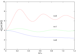
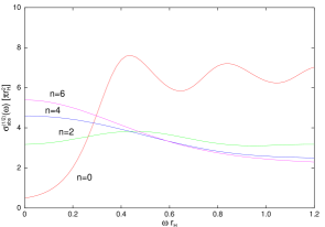
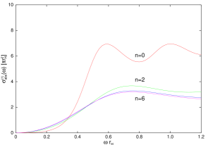
Figure 1: Greybody cross section for brane emission from a (4+n)-dimensional Schwarzschild black hole, for with spin 0, $\frac{1}{2}$ and 1 particles (Reprinted figures with permission from [22]. Copyright SISSA/ISAS 2003).

The results obtained in [22] is shown in Figure 1; we can see that

• greybody factor is a function of particle energy ($\omega$) and spin ($s$);

• greybody factor depends on the number $n$ of extra dimensions, which lead to conclude that it will be possible to “measure” the number of extra dimensions at future colliders ([28], [29], [30]);

• asymptotically the greybody factor tends to geometric optics cross section

  $$\sigma_{g.o.}=\pi\left(\,\frac{n+3}{2}\,\right)^{2/(n+1)}\,\left(\,\frac{n+3}{n+1}\,\right)\,r_{H}^{2}\;,$$ (7)

  because of the finiteness of the gravitational potential barrier, i.e. the potential barrier has a maximum of energy $\omega_{max}$ given by:

  $$\omega_{max}=\frac{1}{r_{H}}\sqrt{\frac{n+1}{n+3}}\,\left(\,\frac{n+3}{2}\,\right)^{-\frac{1}{n+1}}\;.$$ (8)

  When a particle is emitted with an energy $\omega\gtrsim\omega_{max}$ the black hole behaves as an ideal black body with area $\sigma_{g.o.}$.

By integrating equation (2) we can obtain the contribution of spin $s$, Standard Model particle, to $P$ and $F$:

• for $\omega\in[0,\omega_{max}]$, we integrate thermal spectrum (2) with greybody factor $\sigma^{(s)}_{gb}(\omega)$;

• for $\omega\in[\omega_{max},\infty]$, we integrate thermal spectrum (2) with optical geometric cross section $\sigma_{g.o.}$.

Thus, we find

$$P=\left(\frac{dE}{dt}\right)=\frac{1}{2\pi^{2}}\,\int_{0}^{\omega_{max}}d\omega\,\omega^{3}\,\frac{\sigma^{(s)}_{gb}(\omega)}{e^{\omega/T_{BH}}-(-1)^{2s}}+\frac{1}{2\pi^{2}}\,\int_{\omega_{max}}^{\infty}\,d\omega\,\omega^{3}\,\frac{\sigma_{g.o.}\,}{e^{\omega/T_{BH}}-(-1)^{2s}}\;,$$ (9)

and

$$F=\left(\frac{dN}{dt}\right)=\frac{1}{2\pi^{2}}\,\int_{0}^{\omega_{max}}d\omega\,\omega^{2}\,\frac{\sigma^{(s)}_{gb}(\omega)}{e^{\omega/T_{BH}}-(-1)^{2s}}+\frac{1}{2\pi^{2}}\int_{\omega_{max}}^{\infty}d\omega\,\omega^{2}\,\frac{\sigma_{g.o.}}{e^{\omega/T_{BH}}-(-1)^{2s}}\;.$$ (10)

Accounting for color and spin and considering an equal number of particles and antiparticles emitted by black hole, we find the power and flux emitted by a $(4+n)$-dimensional Schwarzschild black hole on brane through different type of Standard Model particles, as reported in Table 1.

Power	$n=0$	$n=2$	$n=4$	$n=6$
Quarks	64,9%	62,9%	61,8%	61,3%
Charged Leptons	10,8%	10,5%	10,3%	10,2%
Neutrinos	5,4%	5,2%	5,2%	5,1%
Photons	1,4%	1,7%	1,8%	1,9%
Gluons	11,3%	13,5%	14,5%	14,9%
Weak bosons	4,3%	5,1%	5,4%	5,6%
Higgs	1,9%	1,0%	1,0%	1,0%

Flux	$n=0$	$n=2$	$n=4$	$n=6$
Quarks	66,5%	64,1%	62,1%	60,8%
Charged Leptons	11,1%	10,7%	10,4%	10,1%
Neutrinos	5,5%	5,3%	5,2%	5,1%
Photons	1,2%	1,5%	1,8%	1,9%
Gluons	9,3%	12,4%	14,1%	15,2%
Weak bosons	3,5%	4,6%	5,3%	5,7%
Higgs	3,1%	1,3%	1,2%	1,2%

Table 1: Power and Flux emitted by a (4+$n$)-dimensional Schwarzschild black hole on brane through Standard Model particles.

We see that $\approx 75$% of decay products are quarks, anti quarks and gluons, while only $\approx 12$% are charged leptons and photons, each particle carrying hundreds GeV of energy. We conclude that the black hole decay is dominated by partons; since they cannot be directly observed, we must to take into account fragmentation into hadrons. Therefore, in next section we are going to study the effects of $QED/QCD$ interactions (not only hadronization) among particles emitted near event horizon, in order to understand what kind of spectra we can expect to detect.

3 QED and QCD Effects

In previous section we have outlined the evaporation process of a mini black hole produced at colliders, with a main focus on the “Schwarzschild Phase”, concluding that brane black hole emission is dominated by quarks and gluons. This emission, which we shall call “direct emission”, consists in the near horizon creation of Standard Model particles through Hawking Mechanism and in their flowing to infinity. However, the picture consisting of Standard Model elementary particles freely escaping to infinity with a black body energy spectrum must be somehow improved by including QCD interaction effects as black hole emission is dominated by quarks and gluons. The inclusion of their interactions is instrumental to build up phenomenologically reliable model predicting the form of the spectrum to be looked for.

In the next section we shall consider in more detail parton fragmentation into hadrons, here we are going to discuss something which could happen before hadronization, i.e. the appearance of a quark-gluon plasma around the black hole ([31], [32]). One starts by considering quarks and gluons emitted according to a black body law. It follows that the parton density near the event horizon grows as $T_{BH}^{3}$. If temperature is high enough, i.e. above some critical value, one expects from $QCD$ quarks and gluons to interact through “bremsstrahlung” and “pair production” processes. These reactions are $2\rightarrow 3$ body processes increasing the number of quarks and gluons nearby black hole and leading to a kind of quark/gluon plasma surrounding the event horizon. While propagating through this plasma quarks and gluons lose energy. When the average energy is low enough partons fragment into hadrons.
Similar arguments can be applied to photons, electrons and positrons as well, provided we replace $QCD$ interactions with the corresponding $QED$ processes. Thus, we can define two distinct regions surrounding the black hole as follows:

• Photosphere, is the spatial region around the black hole where “QED-bremsstrahlung” and “QED-pair production” lead to formation of an $e^{\pm},\gamma$ plasma;

• Chromosphere, is the spatial region around black hole where “QCD-bremsstrahlung” and “QCD-pair production” lead to formation of a quark/gluon plasma.

Spectrum distortion induced by the two “atmospheres” defined above will be discussed in the remaining part of this section.

An analytic description of photosphere and chromosphere dynamics is not available at present; the best one can do is to resort to numerical resolution of Boltzmann equation for the interacting particle distribution function [33]. In order to get a first insight of the phenomena we are considering, we shall introduce a further simplification: we shall use “flat spacetime” diffusion relations even if we are going to study the problem in the geometry of a Schwarzschild black hole.
The number $dn\left(\,\vec{p}\,,r\,\right)$ of particles per unit volume element with momentum between $\vec{p}$ and $\vec{p}+d\vec{p}$ is

$$dn\left(\,\vec{p}\,,r\,\right)=f\left(\,|\,\vec{p}\,|\ ,r\,\right)\,d^{3}p\,r^{2}\,dr\,d\Omega\;,$$

where the distribution function $f\left(\,|\,\vec{p}\,|\ ,r\,\right)$ solves the Boltzmann equation

$$\frac{\partial}{\partial r}f\left(\,p\ ,p_{t}\ ,r\,\right)=\frac{1}{v_{r}}C[f\left(\,p\ ,p_{t}\ ,r\,\right)]\;.$$ (11)

In (11) we introduced the radial velocity $v_{r}$, the transverse component of the momentum $p_{t}$ and defined $p\equiv|\,\vec{p}\,|$. $C[\,f\,]$ is the collision term built out of scattering cross sections encoding information about interactions taking place inside photo and chromosphere.

According to QED (QCD), electrons and positrons (quarks and antiquarks) can lose energy through the emission of photons (gluons): $e^{\pm}e^{\pm}\rightarrow e^{\pm}e^{\pm}\gamma\,(qq\rightarrow qqg).$ Corresponding Feynman diagram is:

brems (80,80) thick i1,i2 o1,o2,o3 fermioni2,v3,o3 photonv2,v3 fermioni1,v2,v1,o2 photonv1,o1 v3

In the ultra-relativistic limit, differential cross section in the center of mass frame reads [34]:

$$\frac{d\sigma}{d\omega}\approx\frac{\alpha^{3}}{E\omega m_{f}^{2}}\left[\frac{4}{3}\left(E-\omega\right)+\frac{\omega^{2}}{E}\right]\times\left[\log\left(\frac{4E^{2}(E-\omega)}{m^{2}_{f}\omega}\right)-\frac{1}{2}\right]\;,$$ (12)

where $m_{f}$ is the fermion mass, $\alpha$ is the electromagnetic (strong) coupling costant, $E$ is the initial energy of each fermion, and $\omega$ is the energy of emitted photon (gluon).
To avoid infra-red divergences, it is convenient to use energy-averaged total cross section ([31], [33]):

$$\sigma\left(\,E\,\right)=\int_{0}^{\infty}\frac{\omega}{E}\left(\,\frac{d\sigma}{d\omega}\,\right)d\omega\approx\frac{\alpha^{3}}{m_{f}^{2}}\log\left(\frac{2E}{m_{f}}\right)\;.$$ (13)

The same type of cross section is obtained for pair production, $e^{\pm}\gamma\rightarrow e^{\pm}e^{+}e^{-}\,(qg\rightarrow q\overline{q}q)$; corresponding Feynman diagram is:

pp (80,80) thick i1,i2 o1,o2,o3 fermioni1,v2,v3,o3 fermiono1,v1,o2 photonv1,v2 photoni2,v3 v3

At order $\alpha^{3}$ one finds:

$$\sigma\left(\,\omega\,\right)\approx\frac{\alpha^{3}}{m_{f}^{2}}\log\left(\frac{2\omega}{m_{f}}\right)\;,$$ (14)

where $\omega$ is the incoming photon (gluon) energy.
Since $\sigma\propto 1/m^{2}_{f}$, heavy fermions minimally affect photo/chromosphere development, and justify photo/chromosphere description in terms of electrons, positrons and light quarks alone, as in [33].

Scattering processes discussed above do not occur in vacuum, rather they take place in an hot plasma of almost-radially moving particles, which is what we call photo/chromosphere. A simple way to take into account finite temperature effects consists in replacing vacuum fermion masses ($m_{f}$ in (13) and (14)) with their thermal counterparts

$$m_{th}^{2}=m_{f}^{2}+M^{2}\left(\,T\,\right)\;,$$ (15)

where $T$ is the plasma temperature and $M$ is often referred to as the plasma mass.
The position (15) gives the propagator pole in momentum space with an accuracy of $10$% [35]. For finite temperature gauge theories, one finds

$$M^{2}\left(\,T\,\right)=g^{2}\,C\left(\,R\,\right)\,\frac{T^{2}}{8}\;,$$

where $g$ is gauge coupling constant, $C(R)$ is the quadratic Casimir invariant for gauge group representation $R$. Relevant values of $C(R)$ in numerical computations [33] are: $C(R)=1$ and $C(R)=4/3$ corresponding to $U(1)$ and $SU(3)$ fundamental representation, respectively. In the hot plasma scenario, fermions move inside photo/chromosphere as “free” particles with a temperature dependent effective mass $m_{th}$.
In next subsection we shall report main results for a numerical resolution of Boltzmann equation (11).

3.1 Numerical Results

Let us start this subsection by investigating formation and development of photo/chromosphere around a four-dimensional Schwarzschild black hole [33], then we shall discuss as photo/chromosphere features depend from the number of extra-dimensions.

3.1.1 Photosphere.

We already mentioned that scattering processes become important only beyond some critical temperature $T_{c}^{QED}$.
Let us introduce $\mathcal{N}(r)$ as the number of collisions a typical particle undergoes between the event horizon and some larger radius $r>r_{H}$. $\mathcal{N}(r)$ can be written in terms of the bremsstrahlung and pair production mean free path, $\lambda(r)$, as

$$\mathcal{N}(r)=\int_{r_{H}}^{r}\frac{dr}{\lambda(r)}\;.$$

We say that a photosphere surrounds the black hole if every particle is scattered at least once between the event horizon and infinity:

$$\lim_{r\rightarrow\infty}\mathcal{N}(r)\geq 1.$$ (16)

Thus, the critical temperature $T_{c}^{QED}$ is the black hole temperature giving one for the limit (16). From numerical analysis we get :

$$T_{c}^{QED}\simeq 50\mbox{ GeV}.$$

Another important photosphere parameter is the inner radius $r_{i}$ which can be defined by $\mathcal{N}\left(\,r_{i}\,\right)=1$, i.e. the mean radial distance for a particle to be scattered once.

Figure 2: Radii for inner photosphere surface for different temperatures; remember that 1 GeV${}^{-1}\simeq 0.197$ fm (Reprinted figure with permission from [33]. Copyright 1999 by The American Physical Society).

Data fit (Figure 2) gives

$$\begin{array}[]{cc}r_{i}=\frac{1}{\kappa T_{BH}},&\kappa=(6.446\pm 0.003)\times 10^{-4}.\\ \end{array}$$ (17)

The inverse dependence from the temperature is due to the fact that bremstrahlung and pair production mean free path decreases with the temperature. Thus, the inner edge of the photosphere is closer to the event horizon. By inserting $r_{H}=\frac{1}{4\pi T_{BH}}$ in (17) we get:

$$r_{i}=\frac{4\pi}{\kappa}r_{H}\simeq 2\times 10^{4}r_{H}.$$ (18)

Even in the case $D\geq 5$, we would not expect a different behavior for inner radius. Indeed, bremsstrahlung and pair production are scattering processes involving Standard Model particles bound to the $D3$-brane.
From an experimental point of view, it is important to know the average final energy $\overline{E}_{f}$ of particles when they start propagating without significant interactions, i.e. the particle average energy at outer photosphere surface, because this is the expected energy to be eventually released in a detecting device.

Figure 3: Particle average energy at outer photosphere surface versus temperature for $T_{BH}\leq 1.5$ TeV (Reprinted figure with permission from [33]. Copyright 1999 by The American Physical Society).

Figure 3 shows $\overline{E}_{f}$ for different black hole temperature $T_{BH}$.

$T_{BH}$ (GeV)	60	300	1000
$\overline{E}_{f}$ (GeV)	$97.0$	$79.5$	$44.2$

Table 2: Average final energy for some values of temperature (Reprinted table with permission from [33]. Copyright 1999 by The American Physical Society).

In Table 2 we report some values extrapolated from Figure 3. Since, in the first approximation, particles are emitted with a black body spectrum, the average energy of a particle close to the event horizon is given by $\overline{E}_{i}\sim 3T_{BH}$; thus, we notice that for $T_{BH}=60$ GeV, $\overline{E}_{f}$ is not much different from $\overline{E}_{i}$, because the temperature is only a little higher than $T_{c}^{QED}$. In this regime the rate of bremsstrahlung and pair production processes is not high enough to decrease in a significant way particle energy. On the other hand, for $T_{BH}=1000$ GeV, $\overline{E}_{f}$ is much smaller than its initial value. These results display in a clear way the role of the photosphere: above a critical temperature the number of particles grows and the average energy decreases. This effect is enhanced at higher black hole temperature. Figure 4 shows up this behavior in a quite evident way.

Figure 4: Particle number versus energy for a 4D Schwarzschild black hole with $T_{BH}=1000$ GeV. (a) : near the horizon. (b) : at the outer photosphere surface (Reprinted figures with permission from [33]. Copyright 1999 by The American Physical Society).

3.1.2 Chromosphere.

By following the same procedure adopted for the photosphere, we find

$$T_{c}^{QCD}\simeq 175\mbox{ MeV}.$$

This result agrees with the analytic estimate in [31]. Thus, we conclude that whenever black hole temperature is high enough to produce a photosphere, then a chromosphere must be present as well. In such a case, the chromosphere inner radius is close to the horizon, i.e. $r_{i}\sim r_{H}$: a black hole with temperature $T_{BH}\gtrsim T_{c}^{QCD}$ emits interacting quarks and gluons in the strong coupling regime with initial black body average energy $\overline{E}_{i}\sim 3T_{BH}$. As they propagate towards infinity their average energy decreases below $\Lambda_{QCD}$ and then fragment into hadrons. In this way, one finds the average final energy for quarks and gluons to be

$$\overline{E}_{f}\sim 200-300\mbox{ MeV}.$$

Transition from partons into hadrons “marks” the position of chromosphere edge. Chromosphere emerging particle spectrum is fairly different from the direct emission spectrum, as there are many more particles with a lower average energy (Figure 5).

Figure 5: Particle number versus energy for a 4D Schwarzschild black hole with $T_{BH}=1.5$ GeV. (a) : Hawking emission spectrum at the horizon and (b) : final spectrum emerging from chromosphere (Reprinted figures with permission from [33]. Copyright 1999 by The American Physical Society).

3.1.3 Concluding Remarks.

Main results obtained in this section can be summarized as follows:

• the presence of a photosphere, or a chromosphere, surrounding the event horizon implies a proliferation of emitted particles; energy conservation leads to a lower average energy per particle. Thus, direct emission spectrum is modified: a black hole with horizon temperature $T_{BH}=1.5$ GeV, effectively behaves as black body at temperature about 100 MeV (Figure 5).
  When emitted particle interactions are properly accounted for, the “free” Hawking spectrum is shifted to a an effective black body spectrum to a temperature lower than the black hole temperature.

• Whenever $T_{BH}\gtrsim\Lambda_{QCD}$, black hole emits quarks and gluons and direct emission is partons dominated (Table 1); furthermore, since $T_{c}^{QCD}\lesssim\Lambda_{QCD}$, strongly coupled quarks and gluons form a chromosphere surrounding the event horizon. Thus, one concludes that final particle spectra will be dominated by hadrons, coming from parton confinement, and their decay products.

Results reported in this section have been obtained in the geometry of a four-dimensional Schwarzschild black hole. However, examining a more general $D$-dimensional case, the following features have to be taken into account:

• scattering processes introduced previously are $D$-independent, because they involve only $3$-Brane confined Standard Model particles; so cross sections (13) and (14) are unaffected;

• brane emission is an intrinsically four-dimensional process, thus, photo/chromosphere dynamics, emitted power, emitted particle number, average initial energy, near horizon particle density don’t change in higher dimensions;

• brane emission is dominated by quarks and gluons independently of $D$, furthermore flux percentages of partons and photons, electrons and positrons, are quite constant.

All these considerations lead us to conclude that the four dimensional picture of black hole decay does not significantly change when moving to higher dimensions.

4 Hadronization and Emergent Spectra

We have seen in previous sections that final spectra, to be measured by an asymptotic observer, are going to be dominated by hadrons, coming from parton confinement, and their decay products, mainly photons, neutrinos and $e^{\pm}$. For this reason, we are going to consider first quarks and gluons hadronization and then black hole emergent spectra in two cases: i) a chromosphere forms and develops; ii) simple near horizon parton hadronization occurs (as in [36]).

In order to recall some usefull formula to study hadronization and hadron decay processes, we are going to determine the $\pi^{0}$ decay photon emergent spectrum.
Let us consider the formation of a neutral, light, $\pi^{0}$ meson. Light mesons, like $\pi^{0}$, represent very likely decay products for heavy hadrons. Furthermore, the preferential decay channel, $\pi^{0}\longrightarrow\gamma+\gamma$, produces two photons which can be easily detected.
Hadronization is an intrinsically non-perturbative effect. As such it is difficult to describe in the framework of $QCD$. Our ignorance about color non-perturbative dynamics can be parametrized in terms of the so-called hadronization function. For a neutral pion the hadronization function reads [33]:

$$\frac{dg_{j\pi}(Q,E_{\pi})}{dE_{\pi}}=\frac{15}{16}\sqrt{\frac{Q}{E_{\pi}^{3}}}\left(1-\frac{E_{\pi}}{Q}\right)^{2}\;,$$ (19)

where $g_{j\pi}(Q,E_{\pi})$ denotes the number of $\pi^{0}$ produced in the energy range $[E_{\pi},E_{\pi}+dE_{\pi}]$ by an energy $Q$ parton of the $j$-th kind. Thus, the flux of neutral pions emitted by a black hole, per unit time, in the energy range $[E_{\pi},E_{\pi}+dE_{\pi}]$ can be written as

$$\frac{dN_{\pi}}{dE_{\pi}dt}=\sum_{j}\int_{E_{\pi}}^{\infty}dQ\frac{dg_{j\pi}(Q\ ,E)}{dE_{\pi}}\,\frac{dN_{j}}{dQdt}\;,$$ (20)

where the sum runs over all the parton species relevant to neutral pion formation.
As mentioned above, we can follow two approaches to clarify the physical meaning of the term $dN_{j}/dQ\,dt$:

• Direct Hadronization: $\frac{dN_{j}}{dQdt}$ denotes the number of $j$-th species partons emitted near the black hole horizon, per unit time, in the energy range between $Q$ and $Q+dQ$, according with a black body spectrum

  $$\frac{dN_{j}}{dQdt}=\frac{\sigma_{gb}^{(s)}(Q)}{\pi^{2}}\frac{Q^{2}}{e^{Q/T_{BH}}-(-1)^{2s}}\;,$$ (21)

  where $s$ is the parton spin, and $\sigma_{gb}^{(s)}$ is the grey-body cross section (Figure 1). Once emitted near the horizon,quarks and gluons freely propagate toward infinity. However, when the relative distance becomes higher than the threshold value $\Lambda_{QCD}^{-1}\sim 1$ fm, then hadronization starts.

• Hadronization after chromosphere formation: differently from the preceeding case, once emitted near the horizon, quarks and gluons propagate toward infinity forming a chromosphere, as discussed previously. Thus, $\frac{dN_{j}}{dQ\,dt}$ denotes the flux of the $j$-th species partons near the outer boundary of the chromosphere; this flux can be evaluated following the method shown in reference [33].

Then, the number of emergent photons, per unit time, in the energy range $[E_{\gamma},E_{\gamma}+dE_{\gamma}]$ is given by

$$\frac{dN_{\gamma}}{dE_{\gamma}dt}=\int_{E_{0}}^{\infty}dE_{\pi}\frac{dg_{\gamma\pi}(E_{\pi},E_{\gamma})}{dE_{\gamma}}\,\frac{dN_{\pi}}{dE_{\pi}dt}\;,$$ (22)

where, $E_{0}=E_{\gamma}+\frac{m_{\pi}^{2}}{4E_{\gamma}}$ is the minimum pion energy which is necessary to produce a photon with energy $E_{\gamma}$, and $m_{\pi}$ is the $\pi^{0}$ mass. The function $\frac{dg_{\gamma\pi}(E_{\pi},E_{\gamma})}{dE_{\gamma}}$ is the number of energy $E_{\gamma}$ photons produced by the decay of a pion with energy $E_{\pi}$ in the laboratory frame:

$$\frac{dg_{\gamma\pi}(E_{\pi},E_{\gamma})}{dE_{\gamma}}=\frac{2}{\sqrt{E_{\pi}^{2}-m_{\pi}^{2}}}\;.$$ (23)

By taking into account equations (19), (20), (22) and (23) one obtains

$$\frac{dN_{\gamma}}{dE_{\gamma}dt}=\sum_{j}\int_{E_{0}}^{\infty}dE_{\pi}\frac{15}{8E_{\pi}^{3/2}\sqrt{E_{\pi}^{2}-m_{\pi}^{2}}}\,\int_{E_{\pi}}^{\infty}dQ\sqrt{Q}\left(1-\frac{E_{\pi}}{Q}\right)^{2}\,\frac{dN_{j}}{dQdt}\;.$$ (24)

This integral can be computed numerically once the partonic flux $\frac{dN_{j}}{dQdt}$ is given according with either of the approaches discussed above.
Equation (24) provides the total flux of photons which can be experimentally detected; these photons are not emitted by the black hole itself but come from the pion decay. Indeed we must to them add the near horizon “direct” emission spectrum. However, also the direct emission photons can lead to the formation of a photosphere through electromagnetic interaction with $e^{\pm}$ and produce a modified spectrum (Figure 4). In what follows, we shall list some results obtained for photon emergent spectra.

4.1 Hadronization “Post-Chromosphere”

In this subsection we shall focus on photon emergent spectra accounting hadronization after chromosphere formation.
Figure 6 shows the total spectrum of photons emitted by a $4D$ Schwarzschild black hole with temperature $T_{BH}=50$ GeV. Both direct emission photons (QED) and $\pi^{0}$ (QCD) decay photons are displayed; each case is considered both when photo/chromosphere is present (solid curve), and when it is absent (dashed curve). The whole photon spectrum is obtained in either case by summing the solid and dashed lines.

Figure 6: Photon emission spectrum for a 4D Schwarzschild black hole with temperature $T_{BH}=50$ GeV. The continuous line denote the spectrum obtained by taking into account the presence of photosphere (QED) and chromosphere (QCD). The dashed lines denote either the direct emission spectrum, or the $\pi^{0}$ (QCD) decay spectrum following near horizon quark hadronization (Reprinted figure with permission from [33]. Copyright 1999 by The American Physical Society).

From Figure 6 one sees that:

• peak energy of $\pi^{0}$ decay photons corresponds to an energy equal to $m_{\pi}/2$; the photon distribution is widened by “Doppler effect” as the pions do not decay at rest;

• according with the previous remark, the photon spectrum in the absence of chromosphere is wider, as the partons do not lose energy in the chromosphere before hadronization;

• the direct emission spectrum is picked around $\sim 5T_{BH}$, while photosphere produces a larger number of photons with smaller energy;

• in the QED sector the photon peak is many orders of magnitude smaller than the photon peak in the QCD sector; as quarks and gluons dominate direct emission, the QCD degrees of freedom, leading to pions, decaying into photons, are many more than direct emission photons. Thus, we conclude that $\pi^{0}$ decay photons dominate the emergent spectrum in Figure 6, both in presence and absence of photo/chromosphere.

Figure 7 shows the decay photon spectrum in the presence of chromosphere (solid line), and the direct emission spectrum (dashed line) from a Schwarzschild black hole in $D=10$ dimensions, for $M_{*}\simeq 1.3$ TeV e $M_{BH}/M_{*}=5$. In this case $T_{BH}\simeq 200$ GeV and the mean life is $\tau_{BH}\simeq 4\times 10^{-27}$s.

Figure 7: Chromosphere emergent photon decay spectrum for a Schwarzschild black hole in $D=10$ dimensions, with $M_{*}\simeq 1.3$ TeV and $M_{BH}/M_{*}=5$. The dashed line shows the direct emission spectrum (Reprinted figure with permission from [37]. Copyright 2003 by The American Physical Society).

A qualitative analysis of Figure 7 shows that the two curves are peaked around $m_{\pi}/2$ (solid line) and $\sim 5T_{BH}$ (dashed line), that is, the involved physical processes (direct emission, chromosphere development, hadronization and $\pi^{0}$ decay) are spacetime dimension independent. This is consistent with the hypothesis that elementary particle interactions are all localized on the spacetime $3$-brane and do not feel the presence of bulk extra dimensions.
We can estimate the number of $\pi^{0}$ decay photons emitted at the outer boundary of the chromosphere to be roughly about $5\cdot 10^{4}$ photons [37]. This number can be improved by adding the photons emerging from the photosphere and the contributions from different hadronic decays.

4.2 Direct Hadronization

In this subsection we shall consider some results regarding final energy spectra accounting direct hadronization.
In order to determine emergent spectra of stable species ($e^{\pm},(\nu\overline{\nu})_{e\mu\tau}$ and in particular $\gamma$), production and decay of a $D$-dimensional Schwarzschild black hole has been numerically performed by using black hole event generator Charybdis v1.001 [38], while both the quark/gluon hadronization and hadronic/leptonic decays have been numerically simulated by Pythia v6.227 [39].
In Table 3 we have reported some parameters obtained for 100 generated events.

$D$	$\langle\,M_{BH}\,\rangle$ (TeV)	$\langle\,T_{BH}\,\rangle$ (GeV)	$\langle\,N_{i}\,\rangle$	$\langle\,N_{f}\,\rangle$	$\langle\,P\,\rangle$
6	10.345 ($\pm$0.030)	140.20 ($\pm$0.13)	19.03 ($\pm$0.23)	1483 ($\pm$26)	78.4 ($\pm$1.4)
7	10.279 ($\pm$0.030)	235.62 ($\pm$0.17)	13.06 ($\pm$0.22)	1244 ($\pm$24)	96.4 ($\pm$1.9)
8	10.31 ($\pm$0.03)	328.43 ($\pm$0.19)	10.80 ($\pm$0.18)	1138 ($\pm$22)	107.1 ($\pm$2.3)
9	10.299 ($\pm$0.027)	416.28 ($\pm$0.18)	9.57 ($\pm$0.18)	1028 ($\pm$22)	109.5 ($\pm$2.5)
10	10.327 ($\pm$0.029)	498.20 ($\pm$0.19)	8.75 ($\pm$0.16)	1014 ($\pm$26)	116.9 ($\pm$2.7)
11	10.259 ($\pm$0.024)	575.37 ($\pm$0.16)	8.19 ($\pm$0.16)	958 ($\pm$22)	120 ($\pm$3)

Table 3: Direct hadronization parameters obtained by 100 generated events. $\langle\,M_{BH}\,\rangle$ and $\langle\,T_{BH}\,\rangle$ are the average mass and temperature of a Schwarzschild black hole produced by Charybdis generator; $\langle\,N_{i}\,\rangle$ is the average number of particles directly emitted by black hole according to the Charybdis simulation, while $\langle\,N_{f}\,\rangle$ is the average number of emergent stable particles after Pythia simulated direct hadronization. $\langle\,P\,\rangle$ is the average production factor, i.e. the number of emergent stable particles following from each particle directly emitted by the black hole.

For different spacetime dimensions $D$, the simulations show that the average black hole mass $\langle\,M_{BH}\,\rangle$ is approximatively costant, while the average temperature $\langle\,T_{BH}\,\rangle$ grows; as a consequence less and less particles are emitted out of the event horizon but they have more and more energy. Thus, the average number of particles directly emitted by black hole $\langle\,N_{i}\,\rangle$ and the average number of emergent stable particles $\langle\,N_{f}\,\rangle$ decrease with $D$, while the average number of emergent stable particles following from each particle directly emitted by the black hole $\langle\,P\,\rangle$ is an increasing function of $D$. Accounting direct hadronization, we can observe that black hole decay has very high multiplicity, i.e. a black hole emits a great number of stable particles of O($10^{3}$).
In Figure 8 we show emergent energy spectra obtained from numerical simulations.

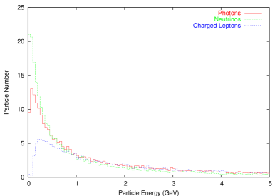
Figure 8: Stable particle energy spectra for a $D=10$-dimensional Schwarzschild black hole accounting direct hadronization.

We notice that the final emergent spectra are dominated by photons and neutrinos. Since future collider detectors are not tuned to capture neutrino signals, a good signature could be missing energy or momentum; thus, in Table 4 we show the average missing energy $\langle\,\cancel{E}\,\rangle$ and the average missing transverse momentum $\langle\,\cancel{p}_{T}\,\rangle$ for several $D$.

$D$	6	8	10
$\langle\,\cancel{E}\,\rangle$ (TeV)	2.65 ($\pm$0.07)	2.63 ($\pm$0.08)	2.55 ($\pm$0.10)
$\langle\,\cancel{p}_{T}\,\rangle$ (TeV)	1.82 ($\pm$0.05)	1.81 ($\pm$0.07)	1.76 ($\pm$0.08)

Table 4: Average missing energy and average missing transverse momentum for a $D$-dimensional Schwarzschild black hole accounting direct hadronization.

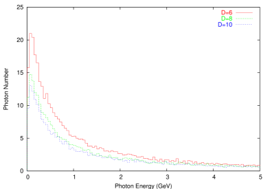
Figure 9: Photon energy spectra for a $D$-dimensional Schwarzschild black hole accounting direct hadronization.

Furthermore, in Figure 9 we show photon energy spectra; since these spectra could be directly observed at future colliders, the whole picture provides a possible experimental signature of TeV mini black hole evaporation.

5 Conclusions

In this article we have reviewed TeV mini black hole decay in models with large extra-dimensions, by taking into account not only the emission of particles according to the Hawking mechanism (referred to as “direct emission”), but near horizon QCD/QED interactions, as well.
We have focused on higher dimensional Schwarzschild black hole decay and we have observed that “brane emission” is parton dominated (see Table 1). Since partons cannot be directly observed, we must take into account fragmentation into hadrons; therefore, in order to understand what kind of spectra we can expect to detect, we have reported emergent photon spectra (Figures 6, 7, 8 and 9), both in the case of more realistic near horizon QCD interactions (parton bremsstrahlung/pair production and after that fragmentation into hadrons) and in the case of “direct hadronization”. Thus, one finds that final emergent spectra, to be measured by an asymptotic observer, are dominated by hadrons and their decay products, mainly neutrinos and photons, both in presence and absence of photo/chromosphere.
In the latter case, we have reported some results obtained by using Charybdis/Pythia event generator package: black hole decay event is characterized by a large multiplicity, as high as $10^{3}$ (see Table 3) and a large missing energy and missing transverse momentum, as high as TeV (see Table 4). The whole picture provides a possible experimental signature at future colliders, as LHC and beyond.
However, much work has still to be done to obtain a phenomenologically reliable signature at collider experiments. For instance, recoil effects of the produced black hole [40], or the influence of Planck phase on the experimental signature ([41], [42]) remain still to be accounted for. In the latter case, according to several theoretical frameworks, it has been argued that the final stage of black hole decay is characterized by a “remnant” formation, i.e. either the black hole temperature abruptly drops to zero [43] or increases up to a maximum temperature and then continuosly approaches an extremal, degenerate configuration at a finite black hole mass ([44],[45],[46]). The effects of this remnant formation on black hole evaporation have been investigated in [42]. The main result is that black hole emits a larger number of Standard Model particles with a lower average energy and transverse momentum than in the case of total evaporation; more in detail, the total trasverse momentum ($\sum p_{T}$) is lowered by a quantity of the order of the remnant mass.
In conclusion, the main feature of black hole decay is the missing of energy or transverse momentum. When a remnant is left after evaporation the missing transverse momentum is of the order of the remnant mass. The big acceptance of the detecting device at LHC will enable a complete event reconstruction and to determine the missing energy. A precise estimate of the missing energy in the framework of a specific regular black hole model is currently under investigation by the authors and the results will be reported elsewhere.

References

- [1] N. Arkani-Hamed, S. Dimopoulos, and G. Dvali. “The hierarchy problem and new dimensions at a millimeter”. Phys. Lett., B429:263–272, 1998. [arXiv:hep-ph/9803315].
- [2] N. Arkani-Hamed, S. Dimopoulos, G. Dvali, and I. Antoniadis. “New dimensions at a millimeter to a Fermi and superstrings at a TeV”. Phys. Lett., B436:257–263, 1998. [arXiv:hep-ph/9804398].
- [3] K. Cheung. “Black hole, string ball and p-brane production at hadronic supercolliders”. Phys. Rev., D66:036007, 2002. [arXiv:hep-ph/0205033].
- [4] S. Hossenfelder, M. Bleicher, and H. Stocker. “Signature of Large Extra Dimensions”. [arXiv:hep-ph/0405031].
- [5] S. B. Giddings and S. Thomas. “High energy colliders as black hole factories: the end of short distance physics”. Phys. Rev., D65:056010, 2002. [arXiv:hep-ph/0106219].
- [6] K. S. Thorne. “Nonspherical Gravitation Collapse: A short Review”. In Magic Without Magic: John Archibald Wheeler. edited by J. R. Klauder, S. Francisco, 1972.
- [7] D. Ida, K. Y. Oda, and S. C. Park. “Rotating black holes at future colliders: greybody factors for brane fields”. Phys. Rev., D67:064026, 2003. [arXiv:hep-th/0212108].
- [8] R. C. Myers and M. J. Perry. “Black holes in higher dimensional space-times”. Ann. Phys., 172:304, 1986.
- [9] D. M. Eardley and S.B.Giddings. “Classical black hole production in high-energy collisions”. Phys. Rev., D66:044011, 2002. [arXiv:gr-qc/0201034].
- [10] H. Yoshino and Y. Nambu. “Black hole formation in the grazing collision of high energy particles”. Phys. Rev., D67:024009, 2003. [arXiv:gr-qc/0209003].
- [11] H. Yoshino and V. S. Rychkov. “Improved analysis of black hole formation in high-energy particle collisions”. [arXiv:hep-th/0503171].
- [12] S. Dimopoulos and G. Landsberg. “Black Hole at the LHC”. Phys. Rev. Lett., 87:161602, 2001. [arXiv:hep-ph/0106295].
- [13] G. Landsberg. “Black Holes at Future Collider and Beyond: a Review”. [arXiv:hep-ph/0211043].
- [14] M. Cavaglia and S. Das. “How Classical are TeV-Scale Black Holes?”. [arXiv:hep-th/0404050].
- [15] S. W. Hawking. “Particles creation by black holes”. Comm. Math. Phys., 43:199–220, 1975.
- [16] E. Spallucci and M. Fontanini. “Zero-point length, extra-dimensions and string T-duality”. In “New Developments in String Theory Research”. S. A. Grece ed., Nova Science Publ., 2005. [arXiv:gr-qc/0508076].
- [17] M. Fontanini, E. Spallucci, and T.Padmanabhan. “Zero-point length from string fluctuations”. [arXiv:hep-th/0509090].
- [18] R. Casadio and B. Harms. “Can black holes and naked singularities be detected in accelerators?”. Int. J. Mod. Phys., A17:4635–4646, 2002. [arXiv:hep-th/0110255].
- [19] D. N. Page. “Particle emission rates from a black hole. II. Massless particles from a rotating hole”. Phys. Rev., D14:3260–3273, 1976.
- [20] R. Emparan, G. T. Horowitz, and R. C. Myers. “Black holes radiate mainly on the brane”. Phys. Rev. Lett., 85:499–502, 2000. [arXiv:hep-th/0003118].
- [21] M. Cavaglia. “Black Hole Multiplicity at particle colliders (Do black holes radiate mainly on the brane?)”. Phys. Lett., B569:7–13, 2003. [arXiv:hep-th/0305256].
- [22] C. M. Harris and P. Kanti. “Hawking radiation from a -dimensional black hole: exact results for the Schwarzschild phase”. JHEP, 0310(014), 2003. [arXiv:hep-ph/0309054].
- [23] P. Kanti and J. March-Russell. “Calculable corrections to brane black hole decay I: the scalar case”. Phys. Rev., D66:024023, 2002. [arXiv:hep-ph/0203223].
- [24] C. W. Misner, K. S. Thorne, and J. A. Wheeler. Gravitation. Freeman and Company, New York, 1973.
- [25] P. Kanti and J. March-Russell. “Calculable corrections to brane black hole decay II: greybody factors for spin 1/2 and 1”. Phys. Rev., D67:104019, 2003. [arXiv:hep-ph/0212199].
- [26] M. Cvetic and F. Larsen. “Greybody factors for black holes in four dimensions: particles with spin”. Phys. Rev., D57:6297–6310, 1998. [arXiv:hep-th/9712118].
- [27] S. S. Gubser, I. R. Klebanov, and A. A. Tseytlin. “String Theory and Classical Absorption by Threebranes”. Nucl. Phys., B499:217–240, 1997. [arXiv:hep-th/9703040].
- [28] P. Kanti. “Black Holes in Theories with Large Extra Dimensions: a Review”. [arXiv:hep-ph/0402168].
- [29] C. M. Harris, M. J. Palmer, M.A. Parker, P. Richardson, A. Sabetfakhry, and B. R. Webber. “Exploring Higher Dimensional Black Holes at the Large Hadron Collider”. JHEP, 0505(053), 2005. [arXiv:hep-ph/0411022].
- [30] J. L. Hewett, B. Lillie, and T. G. Rizzo. “Black holes in many dimension at the LHC: testing critical string theory”. [arXiv:hep-ph/0503178].
- [31] A. F. Heckler. “Formation of a Hawking-radiation photosphere around microscopic black holes”. Phys. Rev., D55:480–488, 1997. [arXiv:astro-ph/9601029].
- [32] A. F. Heckler. “Calculation of the emergent spectrum and observation of primordial black holes”. Phys. Rev. Lett., 78:3430–3433, 1997.
- [33] J. M. Cline, M. Mostoslavsky, and G. Servant. “Numerical study of Hawking radiation photosphere formation around microscopic black holes”. Phys. Rev., D59:063009, 1999. [arXiv:hep-ph/9810439].
- [34] J. M. Jauch and F. Rorhlich. The Theory of Electrons and Photons. Springer-Verlag, New York, 1975.
- [35] H.A. Weldon. “Effective fermion masses of order in high-temperature gauge theories with exact chiral invariance”. Phys. Rev., D26:2789–2796, 1982.
- [36] J. H. MacGibbon and B. R. Webber. “Quark- and gluon-jet emission from primordial black holes: the istantaneous spectra”. Phys. Rev., D41:3052–3079, 1990.
- [37] L. Anchordoqui and H. Goldberg. “Black hole chromosphere at the CERN LHC”. Phys. Rev., D67:064010, 2003. [arXiv:hep-ph/0209337].
- [38] C. M. Harris, P. Richardson, and B. R. Webber. “CHARYBDIS: a black hole event generator”. JHEP, 0308(033), 2003. [arXiv:hep-ph/0307305].
- [39] T. Sj ostrand, L. L onnblad, S. Mrenna, and P. Skands. “Pythia 6.2: Physics and Manual”. [arXiv:hep-ph/0108264].
- [40] A. Flachi and T. Tanaka. “Escape of black holes from the brane”. [arXiv:hep-th/0506145].
- [41] B. Koch, M. Bleicher, and S. Hossenfelder. “Black Hole Remnants at the LHC”. [arXiv:hep-ph/0507138].
- [42] S. Hossenfelder, B. Koch, and M. Bleicher. “Trapping Black Hole Remnants”. [arXiv:hep-ph/0507140].
- [43] R. J. Adler, P. Chen, and D. I. Santiago. “The Generalized Uncertainty Principle and Black Hole Remnants”. Gen.Rel.Grav., 33:2101–2108, 2001. [arXiv:gr-qc/0106080].
- [44] P. Nicolini. “A model of radiating black hole in noncommutative geometry”. J.Phys., A38:L631, 2005. [arXiv:hep-th/0507266].
- [45] P. Nicolini, A. Smailagic, and E. Spallucci. “The fate of radiating black holes in noncommutative geometry”. In “Beyond Einstein, Physics for the 21st Century”. Proceedings of EPS 13 General Conference, University of Bern, Bern, Switzerland, July 11-15, 2005. [arXiv:hep-th/0507226].
- [46] P. Nicolini, A. Smailagic, and E. Spallucci. “Noncommutative geometry inspired Schwarzschild black hole”. [Submitted to PRD].