Preface

D.L. Bennett¹ and H.B. Nielsen^{2 1} Institute of Physics, P.O.Box 57, 11001 Belgrade, Serbia
² Department of Physics, Univ. of Ljubljana, 1000 Ljubljana, Slovenia¹ Educational Faculty, University of Ljubljana, Kardeljeva ploščad 17, 1000 Ljubljana, Slovenia
² Primorska Institute for Natural Sciences and Technology, C. Marežganskega upora 2, 6000 Koper, Slovenia
³ Department of Physics, University of Ljubljana, Jadranska 19, 1000 Ljubljana, Slovenia¹ Department of Physics and Astronomy, Glasgow University, Glasgow, Scotland
² The Niels Bohr Institute, Copenhagen, Denmark¹ Department of Physics, Osaka University, Osaka 560-0043, Japan
² Niels Bohr Institute, University Copenhagen, 17 Blegdamsvej Copenhagen ø, Denmark
³ Yukawa Institute for Theoretical Physics, Kyoto University,Kyoto 606-8502, Japan¹ Faculty of Mathematics and Physics, University of Ljubljana, Jadranska 19, 1000 Ljubljana, Slovenia
² Primorska Institute for Natural Sciences and Technology,
6000 Koper, Slovenia
³ Department of Physics, Niels Bohr Institute, Blegdamsvej 17, Copenhagen, DK-2100¹ Department of Physics, University of Ljubljana, Jadranska 19, 1000 Ljubljana, Slovenia
² Primorska Institute for Natural Sciences and Technology, C. Marežganskega upora 2, 6000 Koper, Slovenia
³ Department of Physics, Niels Bohr Institute, Blegdamsvej 17, Copenhagen, DK-210014U
155 E 34 Street
New York, NY 10016Department of Theoretical Physics, Josef Stefan Institute, Ljubljana, SloveniaDepartment of Mathematics, Polytechnic of Turin, Turin, Italy,Department of Mathematics and Informatics, University of Trieste, Trieste, Italy, INFN, National Institute for Nuclear Physics, Trieste, Italy¹ Niels Bohr Institute, Blegdamsvej 17, Copenhagen, Denmark
² Yukawa Institute for Theoretical Physics, Kyoto University, Kyoto 606-8502, Japan

The series of workshops on ”What Comes Beyond the Standard Model?” started in 1998 with the idea of organizing a real workshop, in which participants would spend most of the time in discussions, confronting different approaches and ideas. The picturesque town of Bled by the lake of the same name, surrounded by beautiful mountains and offering pleasant walks, was chosen to stimulate the discussions.

The idea was successful and has developed into an annual workshop, which is taking place every year since 1998. Very open-minded and fruitful discussions have become the trade-mark of our workshop, producing several published works. It takes place in the house of Plemelj, which belongs to the Society of Mathematicians, Physicists and Astronomers of Slovenia.

In this eight workshop, which took place from 19 to 29 of July 2005 at Bled, Slovenia, we have tried to answer some of the open questions which the Standard models leave unanswered, like:

• Why has Nature made a choice of four (noticeable) dimensions? While all the others, if existing, are hidden? And what are the properties of space-time in the hidden dimensions?

• How could Nature make the decision about the breaking of symmetries down to the noticeable ones, if coming from some higher dimension $d$?

• Why is the metric of space-time Minkowskian and how is the choice of metric connected with the evolution of our universe(s)?

• Why do massless fields exist at all? Where does the weak scale come from?

• Why do only left-handed fermions carry the weak charge? Why does the weak charge break parity?

• What is the origin of Higgs fields? Where does the Higgs mass come from?

• Where does the small hierarchy come from? (Or why are some Yukawa couplings so small and where do they come from?)

• Where do the generations come from?

• Can all known elementary particles be understood as different states of only one particle, with a unique internal space of spins and charges?

• How can all gauge fields (including gravity) be unified and quantized?

• How can different geometries and boundary conditions influence conservation laws?

• Does noncommutativity of coordinate manifest in Nature?

• Can one make the Dirac see working for fermions and bosons?

• What is our universe made out of (besides the baryonic matter)?

• What is the role of symmetries in Nature?

We have discussed these and other questions for ten days. Some results of this efforts appear in these Proceedings. Some of the ideas are treated in a very preliminary way. Some ideas still wait to be discussed (maybe in the next workshop) and understood better before appearing in the next proceedings of the Bled workshops. The discussion will certainly continue next year, again at Bled, again in the house of Josip Plemelj.

Physics and mathematics are to our understanding both a part of Nature. To have ideas how to try to understand Nature, physicists need besides the knowledge also the intuition, inspiration, imagination and much more. Accordingly it is not surprising that there are also poets among us. One of the poems of Astri Kleppe can be found at the end of this Proceedings.

The organizers are grateful to all the participants for the lively discussions and the good working atmosphere.

Norma Mankoč Borštnik
Holger Bech Nielsen
Colin Froggatt
Dragan Lukman

Ljubljana, December 2005

Can MPP Together with Weinberg-Salam Higgs Provide Cosmological Inflation?

D.L. Bennett¹ and H.B. Nielsen^{2 1} Institute of Physics, P.O.Box 57, 11001 Belgrade, Serbia
² Department of Physics, Univ. of Ljubljana, 1000 Ljubljana, Slovenia¹ Educational Faculty, University of Ljubljana, Kardeljeva ploščad 17, 1000 Ljubljana, Slovenia
² Primorska Institute for Natural Sciences and Technology, C. Marežganskega upora 2, 6000 Koper, Slovenia
³ Department of Physics, University of Ljubljana, Jadranska 19, 1000 Ljubljana, Slovenia¹ Department of Physics and Astronomy, Glasgow University, Glasgow, Scotland
² The Niels Bohr Institute, Copenhagen, Denmark¹ Department of Physics, Osaka University, Osaka 560-0043, Japan
² Niels Bohr Institute, University Copenhagen, 17 Blegdamsvej Copenhagen ø, Denmark
³ Yukawa Institute for Theoretical Physics, Kyoto University,Kyoto 606-8502, Japan¹ Faculty of Mathematics and Physics, University of Ljubljana, Jadranska 19, 1000 Ljubljana, Slovenia
² Primorska Institute for Natural Sciences and Technology,
6000 Koper, Slovenia
³ Department of Physics, Niels Bohr Institute, Blegdamsvej 17, Copenhagen, DK-2100¹ Department of Physics, University of Ljubljana, Jadranska 19, 1000 Ljubljana, Slovenia
² Primorska Institute for Natural Sciences and Technology, C. Marežganskega upora 2, 6000 Koper, Slovenia
³ Department of Physics, Niels Bohr Institute, Blegdamsvej 17, Copenhagen, DK-210014U
155 E 34 Street
New York, NY 10016Department of Theoretical Physics, Josef Stefan Institute, Ljubljana, SloveniaDepartment of Mathematics, Polytechnic of Turin, Turin, Italy,Department of Mathematics and Informatics, University of Trieste, Trieste, Italy, INFN, National Institute for Nuclear Physics, Trieste, Italy¹ Niels Bohr Institute, Blegdamsvej 17, Copenhagen, Denmark
² Yukawa Institute for Theoretical Physics, Kyoto University, Kyoto 606-8502, Japan

Abstract

We investigate the possibility of producing inflation with the use of walls rather than the customary inflaton field(s). In the usual picture one needs to fine-tune in such a way as to have at least 60 e-foldings. In the alternative picture with walls that we consider here the “only” fine-tuning required is the assumption of a multiply degenerate vacuum alias the multiple point principle (MPP).

Abstract

We review some new developments in three-dimensional gravity based on Riemann-Cartan geometry. In particular, we discuss the structure of asymptotic symmetry, and clarify its fundamental role in understanding the gravitational conservation laws.

Abstract

In the approach unifying all the internal degrees of freedom - that is the spin and all the charges into only the spin - proposed by one of usABBnorma92 ; ABBnorma93 ; ABBnormasuper94 ; ABBnorma95 ; ABBnorma97 ; ABBpikanormaproceedings1 ; ABBholgernorma00 ; ABBnorma01 ; ABBpikanormaproceedings2 ; ABBPortoroz03 , spinors, living in $d\;(=1+13)-$dimensional space, carry only the spin and interact with only the gravity through spin connections and vielbeins. After a break of symmetries a spin can manifest in $d\;=(1+3)$ ”physical” space as the spin and all the known charges. In this talk we discuss the mass matrices of quarks and leptons, predicted by the approach. Mass matrices follow from the starting Lagrangean, if assuming that there is a kind of breaking symmetry from $SO(1,13)$ to $SO(1,7)\times SU(3)\times U(1)$, which does end up with massless spinors in $d\;(=1+7)$-dimensional space, while a further break leads to mass matrices.

Abstract

We propose that dark matter consists of collections of atoms encapsulated inside pieces of an alternative vacuum, in which the Higgs field vacuum expectation value is appreciably smaller than in the usual vacuum. The alternative vacuum is supposed to have the same energy density as our own. Apart from this degeneracy of vacuum phases, we do not introduce any new physics beyond the Standard Model. The dark matter balls are estimated to have a radius of order 20 cm and a mass of order $10^{11}$ kg. However they are very difficult to observe directly, but inside dense stars may expand eating up the star and cause huge explosions (gamma ray bursts). The ratio of dark matter to ordinary baryonic matter is estimated to be of the order of the ratio of the binding energy per nucleon in helium to the difference between the binding energies per nucleon in heavy nuclei and in helium. Thus we predict approximately five times as much dark matter as ordinary baryonic matter!

Abstract

We consider the long standing problem in field theories of bosons that the boson vacuum does not consist of a ‘sea’, unlike the fermion vacuum. We show with the help of supersymmetry considerations that the boson vacuum indeed does also consist of a sea in which the negative energy states are all “filled”, analogous to the Dirac sea of the fermion vacuum, and that a hole produced by the annihilation of one negative energy boson is an anti-particle. This might be formally coped with by introducing the notion of a double harmonic oscillator, which is obtained by extending the condition imposed on the wave function. Next, we present an attempt to formulate the supersymmetric and relativistic quantum mechanics utilizing the equations of motion.

Abstract

In the approach by one of us (N.S.M.B.)norma ; pikanorma unifying spins and charges, the gauge fields origin only in the gravity and the spins and the charges in only the spin. This approach is also a kind of the genuine Kaluza-Klein theory, suffering the problem of getting chiral fermions in the ”physical space”. In ref.hnhep03 we discussed a possible way for solving this problem by an appropriate choice of boundary conditions. In this contribution we discuss further possible choices of boundary conditions.

Abstract

Using a technique SQCholgernorma2002 ; SQCholgernorma2003 to construct a basis for spinors in terms of the Clifford algebra objects, we define the creation and annihilation operators for spinors and families of spinors as an odd Clifford algebra objects. The proposed ”second quantization” procedure works for all dimensions and any signature and might also help to understand the origin of charges of quarks and leptonsSQCnorma92 ; SQCnorma93 ; SQCnormaixtapa2001 ; SQCpikanorma2003 as well as of their families.

Abstract

Recent developments in physics and mathematics, including group theory and fundamental physics, suggest problems which might provide leads into useful explorations of both physics and mathematics.

Abstract

Adopting noncommutative spacetime coordinates, we determined a new solution of Einstein equations for a static, spherically symmetric matter source. The limitations of the conventional Schwarzschild solution, due to curvature singularities, are overcome. As a result, the line element is endowed of a regular DeSitter core at the origin and of two horizons even in the considered case of electrically neutral, nonrotating matter. Regarding the Hawking evaporation process, the intriguing new feature is that the black hole is allowed to reach only a finite maximum temperature, before cooling down to an absolute zero extremal state. As a consequence the quantum back reaction is negligible.

Abstract

If a macroscopic (random) classical system is put into a random state in phase space, it will of course the most likely have an almost maximal entropy according to second law of thermodynamics. We will show, however, the following theorem: If it is enforced to be periodic with a given period $T$ in advance, the distribution of the entropy for the otherwise random state will be much more smoothed out, and the entropy could be very likely much smaller than the maximal one. Even quantum mechanically we can understand that such a lower than maximal entropy is likely. A corollary turns out to be that the entropy in such closed time-like loop worlds remain constant.

0.1 Introduction

One of the major problems with inflation models in general is that one needs the inflation to go on for very many e-foldings - of the order of sixty - so that the universe can expand by a needed factor of the order of $\exp 60$ while the scalar field causing this inflation remains at roughly the same field value, or at least does not fall down to the present vacuum state value (see for example DBkolbturner ). Accepting the prejudice that the field value should not be larger than the the Planck scale, a normal inflation with an inflaton field would require a rather flat effective potential over a large range of field values but with the restriction that the present vacuum field value should not be further away in field value space than about a Planck energy. This would seemingly suggest a a rather unnatural essentially theta-function-like effective potential. Of course one can with finetuning just postulate that the inflaton effective potential has whatever strange shape may be needed, but it would be nicer if we could instead use some finetuning principle that could also be useful in other contexts.

Now we have for some time worked on the idea of unifying the apparently needed finetunings in the Standard Model (or perhaps some model behind the Standard model) into a single finetuning principle that postulates the coexistence of many vacua or phases with the same cosmological constant namely zero. This is what we called the multiple point principle (MPP)bennett1 ; bennett2 which states that observed coupling constant values correspond to a maximally degenerate vacuum.

The point of the present article is to attempt to find some way to use the finetuning to the degenerate vacua (which is what happens if MPP is assumed) to replace the finetuning otherwise needed to get the rather theta-function-like behavior of the inflaton effective potential. In fact it is not so unlikely that such a replacement of one finetuning by another one could work. We might think about it in the following way:

The essence of what is needed is some field variable $\phi$ - that could be present say as a scalar degree of freedom in any little neighborhood in space - that can simulate the inflaton field. This variable $\phi$ should now be associated with an effective potential - it could be a potential for a Higgs field - having roughly the properties of the inflaton effective potential that are needed needed for a good fitting of inflation. That is to say we should have an effective potential as a function of this scalar field $\phi$ which would behave like the needed theta function. Note that if we restrict ourselves to using only the Standard Model we would have to use as $\phi$ the only scalar field available in the Standard Model namely the Higgs field. Now the characteristics of the many degenrate vacua effective potential for some Higgs field say is that there can, without a need for a volume-proportional energy, be several vacua or phases present in the same spatial regionhbncdf . The energy needed for this is only proportional to an area and not to a volume since all the different vacua have energy density zero. In fact the states that we here refer to consist of two distinct phases separated from one another by a system of walls. Essentially we envision simulating the theta function by having an effective potential that as a function of a degree of freedom corresponding to the distance between phase-delineating walls become “saturated” at some constant value when the distance exceeds some threshold. This essentially means that instead of the usual scenario with inflation in three spatial directions, we instead have lack inflation along one spatial direction. As a consequence, inflation is restricted to taking place along (within)the wall system that make up the boundary between the two (or many more than two in principle) phases.

We speculate about whether there could be, even during an ongoing Hubble expansion, a network of walls that could keep on adjusting itself so as to keep both the energy density and the negative pressure constant so that inflation could be simulated. Such a possibility could come about if the walls expand locally more than the regions between the walls with the result that the average distance between the walls does not have to increase at the same rate under a Hubble expansion as would be the case for isotropic geometrical expansion which would lead to an increase in the distance between the walls by the same factor as time goes on as the expansion along the walls. With this (anisotropic) expansion only along walls we can imagine that the walls must curl up in order to cope with that the average expansion of the whole of space filled with many walls lying in some complicated way is less than the expansion of the walls locally. Such a curling up of walls complicates estimating what really will go on. Hence the possibility for some stabilization of the local density and the revelation of crude features of the wall network is not totally excluded. Most important is that the walls are not driven by forces caused by volume energy density differences - as would generically be the case - because we have assumed the degeneracy of the vacua (our MPP assumption). It is for this reason that the assumption of the multiple point principle leads to wall motion (i.e., field values in the transition region between phases) that is much less strongly driven and in this way mimicks a locally flat effective potential for the inflaton field which is needed phenomenologically to get slow roll. That is to say that the stability and lack of strong forces on the walls allow the walls to develop much more slowly than would be the case without the finetuning provided by the multiple point principle (MPP), and this alone could make a period of inflation simulated by the presence of walls last longer - roll away slower so to speak - than without this MPP. It is in this sense that our finetuning by multiple point prinicple can provide a delay in the disappearance of the inflation-causing features - in our case the walls - that is similiar in effect to having flatness in the effective potential for the inflaton near the point where inflation goes on. The role of this flatness (the theta function plateau) is of course to keep the inflation going over a long time.

So the possibility that the inflation era could be simulated by an era of walls cannot be excluded. Moreover we can even speculate that the assumption of our multiple point principle may even be helpful for getting a more natural way of achieving the slow roll. If we are successful in achieving slow roll in this way, it will of cause only be as a consequence of a finetuning assumption in the form of the multiple point principle instead of the finetuning provided by the clever adjustment of the effective potential that yields slow roll in the usual simple inflation scenario with just a scalar field. However, we have in other works argued that our multiple point principle is useful in providing a explanation for other - perhaps all or at least many - finetuning enigmas in physics. For example it is widely accepted that finetuning is needed in order to account for the extreme smallness of the cosmological constant compared to the huge value which would a priori be expected if one took the Planck units to be the fundamental ones.

A possible model for a system of walls strictly separating two different phases that nevertheless both permeate all of space is provided by structures formed for appropriate parameter values by membranes consisting of amphiphilic molecules. These are the socalled bicontinuous phases - sometimes called the plumber’s nightmare - that for given temperature are observed for sufficiently small values of chemical potentials.

In the scenario of the “plumber’s nightmare”, the labyrinth of “pipe” walls separating the two phases proliferates in such a way that the volume between pipe walls remains constant on average while the “nightmare” as a whole expands.

0.2 Can it work?

It is not yet clear that one can replace an inflation period with a simple scalar field taking a constant value by a situation with an effective potential that depends on field degrees of freedom corresponding to the distance between walls that separate two (or more) degenerate vacua having the same (vanishing) energy density. Of course if the cosmological constant for the vacua corresponding to the bottoms of the potentials were not essentially zero (we take the tiny cosmological constant of today as being essentially zero, because we are interested in the early era of inflation when the inflation was enormous compared to what could be achieved by today’s cosmological constant) we could still get inflation, but here our idea is to obtain the inflation due to the walls, which means due to the scalar field potential in the transition regions - the walls - between the two phases. If we can ignore the effects of the field gradients which are of course non-zero in the wall regions too, there would be an inflation effect coming simply from the walls. It would just be reduced by the ratio of the wall volume to the full volume one could say compared to the inflation that would be obtained by having the inflaton field just sitting on the maximum of the effective potential between the two minima corresponding to the two vacua. The gradient in the direction perpendicular to the walls will then give a contribution to the energy momentum tensor which depends on the direction and when averaged over directions contribute more energy relative to pressure than the cosmological constant or equivalently constant scalar field terms.

Let us for our purposes optimistically imagine that during the main era of inflation we have the situation that, compared to the spaces in between the walls, the walls themselves get bigger and bigger areas. Then the wall density would seem at first quite likely to increase with time and the walls might even curl up or even collide and interact with each other. In this scenario the energy density might even seem to have the possibility of increasing. Really however the overall expansion will diminish the energy density because the negative pressure is not high enough to compensate.

Now we may ask which effects will come to dominate when the density is respectively high or low. If the density is low one would say that each piece of wall will be isolated in first approximation and the expansion of the wall area will go on while the distance to the next wall hardly will change significantly percentwise. That suggests that in the low density case we would expect that the local expansion of the walls forcing them to curl up will dominate. This in turn will cause the density to become higher.

On the other hand, if the density is high, then the network of walls makes up a kind of complicated matter. Adjacent walls are not isolated from one another; they now “feel” one another and it must be justifiable to use the approximation that the main effect of the Hubble expansion can be assumed to be the effect on this matter. therefore the expansion will be isotropic (and not just along the walls) provided the “network of walls is on the average isotropic. In this case the effect of total expansion dominates. That would cause the density of walls to fall as under simple Hubble expansion in which the single wall plays no important role.

Using these two estimates we then see that the density will tend to be driven to some intermediate density as the inflation-like Hubble expansion goes on. If the density becomes too low it will tend to grow, and if too high it will fall. If such a stabilization indeed takes place the density will reach an intrmediate stable level.

Once the stable density has been reached the Hubble constant will become constant and in this sense we will then have obtained a situation that even in the mathematical form for the expansion - exponential form - will simulate the usual simple inflation for a constant scalar inflaton field. The constant Hubble expansion constant referred to above is really the average Hubble expansion - denote it by $H_{av}$ - of the bulk system of walls as well as the space in between. $H_{av}$ is to be distinguished from the Hubble expansion along the walls - let us denote this as $H_{wall}$. Recall that we expect that $H_{av}<H_{wall}$ - also at the stable wall density value.

Then denoting the the ratio of the total volume to the part of it taken up by the walls by $\xi$

$$\xi=\frac{``\hbox{full \quad volume''}}{\hbox{``wall-volume''}}$$ (1)

we have that the Hubble expansion in the wall-regions $H_{wall}$ is bigger than outside by a factor $\xi$,

$$H_{wall}=\sqrt{\xi}H_{av}.$$ (2)

0.3 What is the stabile wall density?

If indeed such a speculated stabilization takes place, we may make a dimensionality argument for what the stability density will be.

Let us take the picture that the walls are topologically stabilized and therefore unable to decay everywhere except where they collide with each other. Roughly we expect the walls to be about to cross in a fraction $1/\xi^{2}$ of the total space or in a fraction $1/\xi$ of the wall-space. We need an estimate as to how fast this wall interaction region gets turned into being one or the other of the vacuum phases by the decay of its energy into other types of particles. This is what is usually supposed to happen during reheating in normal inflation models - namely that pairs of non-inflaton particles are produced during the decay of the scalar particle involved in the inflation. We shall also in our picture imagine that such a reheating-like mechanism is going on. For dimensional reasons we expect the typical energy scale for the field $\phi$ at the wall to give the scale for the decay rate. This wall-scale is say the maximal value of the effective potential for $\phi$ in the interval between the two minima. This scale we could call $V_{max}$ or $V_{wall}$ because it is also the typical value of the effective potential $V_{eff}$ in the wall-volume. We must admit though that strictly speaking the scale that would be most relevant for the reheating decay rate would be the mass scale of the $\phi$-particle which decays or some effective mass scale denoting the energy of a state for this particle as a bound state in the surrounding fields. A rough estimate for this mass scale would be the square root of the second derivative of the effective potential, mass $\approx\sqrt{V_{eff}^{\prime\prime}}$. As an estimate for this we might take an expression involving the difference $\phi_{vac1}-\phi_{vac2}$ between the $\phi$-values for the say two minima, $\phi_{vac1}$ and $\phi_{vac2}$. In fact we estimate $V_{eff}^{\prime\prime}\approx V_{wall}/(\phi_{vac1}-\phi_{vac2})^{2}$. Therefore the better mass scale to use would be $\sqrt{V_{wall}}/|\phi_{vac1}-\phi_{vac2}|$. Let us take the decay rate - i.e. the inverse of the time scale for the decay of the field to its locally topologigally stable situation - to be:

$$\hbox{``decay rate ''}\approx n\frac{\sqrt{V_{wall}}}{|\phi_{vac1}-\phi_{vac2}|}.$$ (3)

Here $n$ is a dimensionless quantity that is essentailly the number of decay channels weighted by the appropriate products of coupling constants.

To have stability we now have to have that the amount of walls produced percentwise from the Hubble expansion of the walls (which is roughly $H_{wall}$) should be in balance with the destruction rate which percentwise becomes

$$n\frac{\sqrt{V_{wall}}}{|\phi_{vac1}-\phi_{vac2}|\xi}.$$

I.e. we have

$$H_{wall}\approx n\frac{\sqrt{V_{wall}}}{|\phi_{vac1}-\phi_{vac2}|\xi}.$$ (4)

If we took all the coupling constants to be of order unity and included only two-particle decays with all the selection rules ignored, the number $n$ of decay channels would of course be the square of the number of particle species into which the $\phi$-particle could decay. Denoting this number by $n_{s}$ (where s stands for “species”), we get $n=n_{s}^{2}$.

If in the philosophy of taking the scale for the scalar field to be of the Planck energy scale we take $|\phi_{vac1}-\phi_{vac2}|\approx 1$ (in Planck units), then we get in these Planck units $H_{wall}\approx n\sqrt{V_{wall}}/\xi$, or using $H_{wall}\approx\sqrt{V_{wall}}$ as is true in Planck units, i. e. we get $\xi\approx n$.

0.4 How did the present Universe come about?

Our wall-dominated model for slow roll must of course contain the ultimate demise of these walls because a wall-dominated Universe is not what we see today. A first glance this might seem to be a problem since MPP says that the different vacua are degenerate and therefore there is not a dominant or preferred phase that can squeeze all other phases out of existence and thereby eliminate the walls that delineate these weaker phases.

However, while MPP claims degeneracy of multiple vacua primordially and during inflation, it does not stipulate that there is a symmetry between the different degenerate vacua. Different phases (i.e., degenerate vacua) could for example differ in having heavier or lighter particles in which case the addition of heat at the end of the inflationary era would reveal the assymmetries of the phases e.g., the phase with lightest degrees of freedom would due to the $-TS$ term in the free energy grow in spatial extent at the expense of phases with heavier degrees of freedom. Concurrent with the disappearence of these phases with heavier degrees of freedom the walls delineating them would also disappear. But during the inflation period in which the temperature is effectively zero the phase assymmetries are hidden and the conditions for having delineating walls separating effectively symmetric (and degenerate) phases are plausibly good.

0.5 Conclusion

We propose that the inflationary era of the Universe was dominated by a network of walls separating degenerate vacua. Assuming such a multidegenerate vacuum is equivalent to assuming the validity of our multiple point principle (MPP). The assumption of MPP amounts to a finetuning to this multiply degenerate vacuum and as such is to be regarded as an alternative to the usual fintuning necessary for having a constant value of the inflaton potential for a scalar field for of the order of 60 e-foldings.

It is conjectured that this inflation era wall density is stabilized such that for too low a density Hubble expansion occurs predominantly along the walls (and essentially not within the phase volume delineated by the walls). This would lead to a corrective increase in wall density to the stable value. If the wall density were to exceed the stable density value, the walls are no longer isolated from one another with the result that the presumeably isotropic wall network materia is subject to an isotropic (bulk) Hubble expansion. Such an expansion of this bulk materia would tend to reduce the wall density until the stabile wall density is attained

While phases separated by the walls are degenerate (and assumed to all have a vanishing energy density) they need not be symmetric. Such assymmetris while being effectively hidden during inflation can be manifested during reheating at the end of the era of inflation. So two phases could for example differ in having lighter and heavier degrees of freedom respectively. This assymmetry would during reheating be manifested as a difference in the free energy of the two phases so that only one phase would survive. The other phase would be obliterated together with the wall network system that separated the two phases during the inflationary era. Disappearence of the walls is of course required by the phenomenology of our present day Universe.

Conserved Charges in 3d Gravity With Torsion M. Blagojević^1,2 and B. Cvetković¹

0.6 Introduction

Although general relativity (GR) successfully describes all the known observational data, such fundamental issues as the nature of classical singularities and the problem of quantization remain without answer. Faced with such difficulties, one is naturally led to consider technically simpler models that share the same conceptual features with GR. A particularly useful model of this type is three-dimensional (3d) gravity mbbc1 . Among many interesting results achieved in the last twenty years, we would like to mention (a) the asymptotic conformal symmetry of 3d gravity, (b) the Chern-Simons formulation, (c) the existence of the black hole solution, and (d) understanding of the black hole entropy mbbc2 ; mbbc3 ; mbbc4 ; mbbc5 .

Following a widely spread belief that GR is the most reliably approach to describe the gravitational phenomena, 3d gravity has been studied mainly in the realm of Riemannian geometry. However, there is a more general conception of gravity, based on Riemann-Cartan geometry mbbc6 , in which both the curvature and the torsion are used to describe the gravitational dynamics. In this review, we focus our attention on some new developments in 3d gravity, in the realm of Riemann-Cartan geometry mbbc7 ; mbbc8 ; mbbc9 ; mbbc10 ; mbbc11 . In particular, we show that the symmetry of anti-de Sitter asymptotic conditions is described by two independent Virasoro algebras with different central charges, in contrast to GR, and discuss the importance of the asymptotic structure for the concept of conserved charges—energy and angular momentum mbbc10 .

0.7 Basic dynamical features

Theory of gravity with torsion can be formulated as Poincaré gauge theory (PGT), with an underlying geometric structure described by Riemann-Cartan space mbbc6 .

PGT in brief. Basic gravitational variables in PGT are the triad field $b^{i}$ and the Lorentz connection $A^{ij}=-A^{ji}$ (1-forms). The corresponding field strengths are the torsion and the curvature: $T^{i}=db^{i}+A^{i}{{}_{m}}\wedge b^{m}$, $R^{ij}=dA^{ij}+A^{i}{{}_{m}}\wedge A^{mj}$ (2-forms). Gauge symmetries of the theory are local translations and local Lorentz rotations, parametrized by $\xi^{\mu}$ and $\varepsilon^{ij}$.

In 3D, we can simplify the notation by introducing

$$A^{ij}=-\varepsilon^{ijk}\omega_{k}\,,\qquad R^{ij}=-\varepsilon^{ijk}R_{k}\,,\qquad\varepsilon^{ij}=-\varepsilon^{ijk}\theta_{k}\,.$$

In local coordinates $x^{\mu}$, we have $b^{i}=b^{i}{{}_{\mu}}dx^{\mu}$, $\omega^{i}=\omega^{i}{{}_{\mu}}dx^{\mu}$. The field strengths take the form

$$T^{i}=db^{i}+\varepsilon^{i}{}_{jk}\omega^{j}\wedge b^{k}=\frac{1}{2}T^{i}{}_{\mu\nu}dx^{\mu}\wedge dx^{\nu}\,,$$

$$R^{i}=d\omega^{i}+\frac{1}{2}\,\varepsilon^{i}{}_{jk}\omega^{j}\wedge\omega^{k}=\frac{1}{2}R^{i}{}_{\mu\nu}dx^{\mu}\wedge dx^{\nu}\,,$$ (1)

and gauge transformations are given as

$$\delta_{0}b^{i}{{}_{\mu}} = -\varepsilon^{i}{}_{jk}b^{j}{}_{\mu}\theta^{k}-(\partial_{\mu}\xi^{\rho})b^{i}{{}_{\rho}}-\xi^{\rho}\partial_{\rho}b^{i}{}_{\mu}\equiv\delta_{\scriptstyle\rm PGT}b^{i}{}_{\mu}\,,$$

$$\delta_{0}\omega^{i}{{}_{\mu}} = -\nabla_{\mu}\theta^{i}-(\partial_{\mu}\xi^{\rho})\omega^{i}{{}_{\rho}}-\xi^{\rho}\partial_{\rho}\omega^{i}{}_{\mu}\equiv\delta_{\scriptstyle\rm PGT}\omega^{i}{}_{\mu}\,,$$ (2)

where $\nabla_{\mu}\theta^{i}=\partial_{\mu}\theta^{i}+\varepsilon^{i}{}_{jk}\omega^{j}{{}_{\mu}}\theta^{k}$ is the covariant derivative of $\theta^{i}$.

To clarify the geometric meaning of PGT, we introduce the metric tensor as a bilinear combination of the triad fields:

$$g=\eta_{ij}b^{i}\otimes b^{j}\equiv g_{\mu\nu}dx^{\mu}\otimes dx^{\nu}\,,\qquad\eta_{ij}=(+,-,-)\,.$$

Although metric and connection are in general independent geometric objects, in PGT they are related to each other by the metricity condition: $\nabla g=0$. Consequently, the geometric structure of PGT is described by Riemann-Cartan geometry. Using the metricity condition, one can derive the useful identity

$$\omega^{i}={\widetilde{\omega}}^{i}+K^{i}\,,$$ (3)

where ${\widetilde{\omega}}^{i}$ is Riemannian connection, $K_{ijk}=-\frac{1}{2}(T_{ijk}-T_{kij}+T_{jki})$ is the contortion, and $K^{i}$ is defined by $K^{ij}{{}_{m}}b^{m}\equiv K^{ij}=-\varepsilon^{ijk}K_{k}$.

Topological action. General gravitational dynamics is defined by Lagrangians which are at most quadratic in field strengths. Omitting the quadratic terms, Mielke and Baekler proposed a topological model for 3D gravity mbbc7 , defined by the action

$$I=aI_{1}+\Lambda I_{2}+\alpha_{3}I_{3}+\alpha_{4}I_{4}+I_{M}\,,$$ (4a)

where

$$I_{1}\equiv 2\int b^{i}\wedge R_{i}\,,$$

$$I_{2}\equiv-\frac{1}{3}\,\int\varepsilon_{ijk}b^{i}\wedge b^{j}\wedge b^{k}\,,$$

$$I_{3}\equiv\int\left(\omega^{i}\wedge d\omega_{i}+\frac{1}{3}\varepsilon_{ijk}\omega^{i}\wedge\omega^{j}\wedge\omega^{k}\right)\,,$$

$$I_{4}\equiv\int b^{i}\wedge T_{i}\,,$$ (4b)

and $I_{M}$ is a matter contribution. The first term, with $a=1/16\pi G$, is the usual Einstein-Cartan action, the second term is a cosmological term, $I_{3}$ is the Chern-Simons action for the Lorentz connection, and $I_{4}$ is a torsion counterpart of $I_{1}$. The Mielke-Baekler model is a natural generalization of Riemannian GR with a cosmological constant (GR_Λ).

Field equations. Variation of the action with respect to $b^{i}$ and $\omega^{i}$ yields the gravitational field equations. In order to understand the canonical structure of the theory in the asymptotic region, it is sufficient to consider the field equations in vacuum (for isolated gravitational systems, gravitational sources can be practically ignored in the asymptotic region). In the sector $\alpha_{3}\alpha_{4}-a^{2}\neq 0$, these equations take the simple form

$$2T^{i}=p\varepsilon^{i}{}_{jk}\,b^{j}\wedge b^{k}\,,\qquad 2R^{i}=q\varepsilon^{i}{}_{jk}\,b^{j}\wedge b^{k}\,,$$ (5)

where

$$p=\frac{\alpha_{3}\Lambda+\alpha_{4}a}{\alpha_{3}\alpha_{4}-a^{2}}\,,\qquad q=-\frac{(\alpha_{4})^{2}+a\Lambda}{\alpha_{3}\alpha_{4}-a^{2}}\,.$$

Thus, the vacuum solution is characterized by constant torsion and constant curvature. For $p=0$, the vacuum geometry is Riemannian ($T^{i}=0$), while for $q=0$, it becomes teleparallel ($R^{i}=0$).

In Riemann-Cartan spacetime, one can use the identity (2.3) to express the curvature $R^{i}(\omega)$ in terms of its Riemannian piece ${\tilde{R}}^{i}\equiv R^{i}({\widetilde{\omega}})$ and the contortion: $R^{i}(\omega)={\tilde{R}}^{i}+\nabla K^{i}-\frac{1}{2}\varepsilon^{imn}K_{m}\wedge K_{n}$. This result, combined with the field equations (5), leads to

$$2{\tilde{R}}^{i}=\hbox{$\mit\Lambda_{\hskip 0.6pt\rm eff}$}\,\varepsilon^{i}{}_{jk}\,b^{j}\wedge b^{k}\,,\qquad\hbox{$\mit\Lambda_{\hskip 0.6pt\rm eff}$}\equiv q-\frac{1}{4}p^{2}\,,$$ (6)

where $\mit\Lambda_{\hskip 0.6pt\rm eff}$ is the effective cosmological constant. Consequently, our spacetime is maximally symmetric: for $\hbox{$\mit\Lambda_{\hskip 0.6pt\rm eff}$}<0$ ($\hbox{$\mit\Lambda_{\hskip 0.6pt\rm eff}$}\geq 0$), the spacetime manifold is anti-de Sitter (de Sitter/Minkowski). In what follows, our attention will be focused on the model (4) with $\alpha_{3}\alpha_{4}-a^{2}\neq 0$, and with negative $\mit\Lambda_{\hskip 0.6pt\rm eff}$ (anti-de Sitter sector):

$$\hbox{$\mit\Lambda_{\hskip 0.6pt\rm eff}$}\equiv-\frac{1}{\ell^{2}}<0\,.$$ (7)

0.8 The black hole solution

For $\hbox{$\mit\Lambda_{\hskip 0.6pt\rm eff}$}<0$, equation (6) has a well known solution for the metric — the BTZ black hole. Using the static coordinates $x^{\mu}=(t,r,\varphi)$ with $0\leq\varphi<2\pi$, the black hole metric is given by

$$ds^{2}=N^{2}dt^{2}-N^{-2}dr^{2}-r^{2}(d\varphi+N_{\varphi}dt)^{2}\,,$$

$$N^{2}=\left(-8Gm+\frac{r^{2}}{\ell^{2}}+\frac{16G^{2}J^{2}}{r^{2}}\right)\,,\qquad N_{\varphi}=\frac{4GJ}{r^{2}}\,,$$ (1)

with $m\geq 0$, $\ell m\geq|J|$. If $r_{+}$ and $r_{-}$ are the zeros of $N^{2}$, then we have: $m=(r_{+}^{2}+r_{-}^{2})/8G\ell^{2}$, $J=r_{+}r_{-}/4G\ell$. The relation between the parameters $m,J$, and the black hole energy and angular momentum, will be clarified later. Since the triad field corresponding to (1) is determined only up to a local Lorentz transformation, we can choose $b^{i}$ to have the simple form:

$$b^{0}=Ndt\,,\qquad b^{1}=N^{-1}dr\,,\qquad b^{2}=r\left(d\varphi+N_{\varphi}dt\right)\,.$$ (2a)

To find the connection, we combine the relation $$K^{i}=(p/2)b^{i}$$, which follows from the first field equation in (5), with the identity (3). This yields

$$\omega^{i}={\widetilde{\omega}}^{i}+\frac{p}{2}\,b^{i}\,,$$ (2b)

where the Riemannian connection $${\widetilde{\omega}}^{i} d{\widetilde{\omega}}^{i}+\varepsilon^{i}{}_{jk}{\widetilde{\omega}}^{j}b^{k}=0$$ is defined by :

$${\widetilde{\omega}}^{0}=-Nd\varphi\,,\qquad{\widetilde{\omega}}^{1}=N^{-1}N_{\varphi}dr\,,\qquad{\widetilde{\omega}}^{2}=-\frac{r}{\ell^{2}}dt-rN_{\varphi}d\varphi\,.$$ (2c)

Equations (2) define the BTZ black hole in Riemann–Cartan spacetime mbbc8 ; mbbc9 . As a constant curvature spacetime, the black hole is locally isometric to the AdS solution (AdS₃), obtained formally from (2) by the replacement $J=0$, $8Gm=-1$.

0.9 Asymptotic conditions

For isolated gravitational systems, matter is absent from the asymptotic region. In spite of that, it can influence global properties of spacetime through the asymptotic conditions, the symmetries of which are closely related to the gravitational conserved charges mbbc10 .

AdS asymptotics. For $\hbox{$\mit\Lambda_{\hskip 0.6pt\rm eff}$}<0$, maximally symmetric AdS solution has the role analogous to the role of Minkowski space in the $\hbox{$\mit\Lambda_{\hskip 0.6pt\rm eff}$}=0$ case. Following the analogy, we could choose that all the fields approach the single AdS₃ configuration at large distances. The asymptotic symmetry would be the global AdS symmetry $SO(2,2)$, the action of which leaves the AdS₃ configuration invariant. However, this choice would exclude the important black hole solution. This motivates us to introduce the asymptotic AdS configurations, determined by the following requirements:

• the asymptotic conditions include the black hole configuration,

• they are invariant under the action of the AdS group, and

• the asymptotic symmetries have well defined canonical generators.

The asymptotics of the triad field $b^{i}{{}_{\mu}}$ that satisfies (a) and (b) reads:

$$b^{i}{{}_{\mu}}=\left(\begin{array}[]{ccc}\displaystyle\frac{r}{\ell}+{\cal O}_{1}&O_{4}&O_{1}\\ {\cal O}_{2}&\displaystyle\frac{\ell}{r}+{\cal O}_{3}&O_{2}\\ {\cal O}_{1}&{\cal O}_{4}&r+{\cal O}_{1}\end{array}\right)\,.$$ (1a)

Here, for any $${\cal O}_{n}=c/r^{n} c t \varphi c=c(t,\varphi) SO(2,2)$$, we assume that is not a constant, but a function of and , , which is the simplest way to ensure the global invariance. This assumption is of crucial importance for highly non-trivial structure of the resulting asymptotic symmetry.

The asymptotic form of $\omega^{i}{{}_{\mu}}$ is defined in accordance with (2b):

$$\omega^{i}{{}_{\mu}}=\left(\begin{array}[]{ccc}\displaystyle\frac{pr}{2\ell}+{\cal O}_{1}&{\cal O}_{4}&\displaystyle-\frac{r}{\ell}+{\cal O}_{1}\\ {\cal O}_{2}&\displaystyle\frac{p\ell}{2r}+{\cal O}_{3}&{\cal O}_{2}\\ \displaystyle-\frac{r}{\ell^{2}}+{\cal O}_{1}&{\cal O}_{4}&\displaystyle\frac{pr}{2}+{\cal O}_{1}\end{array}\right)\,.$$ (1b)

A verification of the third condition (c) is left for the next section.

Asymptotic parameters. Having chosen the asymptotic conditions, we now wish to find the subset of gauge transformations (2) that respect these conditions. They are defined by restricting the original gauge parameters in accordance with (1), which yields

$$\xi^{0}=\ell\left[T+\frac{1}{2}\left(\frac{\partial^{2}T}{\partial t^{2}}\right)\frac{\ell^{4}}{r^{2}}\right]+{\cal O}_{4}\,,\qquad\xi^{1}=-\ell\left(\frac{\partial T}{\partial t}\right)r+{\cal O}_{1}\,,$$

$$\xi^{2}=S-\frac{1}{2}\left(\frac{\partial^{2}S}{\partial\varphi^{2}}\right)\frac{\ell^{2}}{r^{2}}+{\cal O}_{4}\,,$$ (2a)

and

$$\theta^{0}=-\frac{\ell^{2}}{r}\partial_{0}\partial_{2}T+{\cal O}_{3}\,,\qquad\theta^{1}=\partial_{2}T+{\cal O}_{2}\,,$$

$$\theta^{2}=\frac{\ell^{3}}{r}\partial_{0}^{2}T+{\cal O}_{3}\,.$$ (2b)

The functions $T$ and $S$ are such that $\partial_{\pm}(T\mp S)=0$, with $x^{\pm}\equiv x^{0}/\ell\pm x^{2}$, which implies

$$T+S=g(x^{+})\,,\qquad T-S=h(x^{-})\,,$$

where $g$ and $h$ are two arbitrary, periodic functions.

The commutator algebra of the Poincaré gauge transformations (2) is closed: $[\delta_{0}^{\prime},\delta_{0}^{\prime\prime}]=\delta_{0}^{\prime\prime\prime}$, where $\delta_{0}^{\prime}=\delta_{0}(\xi^{\prime},\theta^{\prime})$ and so on. Using the related composition law with the restricted parameters (2), and keeping only the lowest order terms, one finds the relation

$$T^{\prime\prime\prime}=T^{\prime}\partial_{2}S^{\prime\prime}+S^{\prime}\partial_{2}T^{\prime\prime}-T^{\prime\prime}\partial_{2}S^{\prime}-S^{\prime\prime}\partial_{2}T^{\prime}\,,$$

$$S^{\prime\prime\prime}=S^{\prime}\partial_{2}S^{\prime\prime}+T^{\prime}\partial_{2}T^{\prime\prime}-S^{\prime\prime}\partial_{2}T^{\prime}-T^{\prime\prime}\partial_{2}ST^{\prime}\,,$$ (3)

which is expected to be the composition law for $(T,S)$. To verify this assumption, we separate the parameters (2) into two pieces: the leading terms containing $T$ and $S$ define a $(T,S)$ transformation, while the rest defines the residual (pure gauge) transformation. The PGT commutator algebra implies that the commutator of two $(T,S)$ transformations produces not only a $(T,S)$ transformations, but also an additional pure gauge transformation. This result motivates us to introduce an improved definition of the asymptotic symmetry: it is the symmetry defined by the parameters (2), modulo pure gauge transformations. As we shall see in the next section, this symmetry coincides with the conformal symmetry.

0.10 Canonical generators and conserved charges

In this section, we continue our study of the asymptotic symmetries and conservation laws in the canonical formalism mbbc10 .

Hamiltonian and constraints. Introducing the canonical momenta $(\pi_{i}{{}^{\mu}},\Pi_{i}{{}^{\mu}})$, corresponding to the Lagrangian variables $(b^{i}{{}_{\mu}},\omega^{i}{{}_{\mu}})$, we find that the primary constraints of the theory (4) are of the form:

$$\phi_{i}{{}^{0}}\equiv\pi_{i}{{}^{0}}\approx 0\,,\hskip 82.5pt\Phi_{i}{{}^{0}}\equiv\Pi_{i}{{}^{0}}\approx 0\,,$$

$$\phi_{i}{{}^{\alpha}}\equiv\pi_{i}{{}^{\alpha}}-\alpha_{4}\varepsilon^{0\alpha\beta}b_{i\beta}\approx 0\,,\qquad\Phi_{i}{{}^{\alpha}}\equiv\Pi_{i}{{}^{\alpha}}-\varepsilon^{0\alpha\beta}(2ab_{i\beta}+\alpha_{3}\omega_{i\beta})\approx 0\,.$$

Up to an irrelevant divergence, the total Hamiltonian reads

$${\cal H}_{T}=b^{i}{{}_{0}}{\cal H}_{i}+\omega^{i}{{}_{0}}{\cal K}_{i}+u^{i}{{}_{0}}\pi_{i}{{}^{0}}+v^{i}{{}_{0}}\Pi_{i}{{}^{0}}\,,$$ (1)

$${\cal H}_{i}=-\varepsilon^{0\alpha\beta}\left(aR_{i\alpha\beta}+\alpha_{4}T_{i\alpha\beta}-\Lambda\varepsilon_{ijk}b^{j}{{}_{\alpha}}b^{k}{{}_{\beta}}\right)$$

$$\hskip 141.0pt-\nabla_{\beta}\phi_{i}{{}^{\beta}}+\varepsilon_{imn}b^{m}{{}_{\beta}}\left(p\phi^{n\beta}+q\Phi^{n\beta}\right)\,,$$

$${\cal K}_{i}=-\varepsilon^{0\alpha\beta}\left(aT_{i\alpha\beta}+\alpha_{3}R_{i\alpha\beta}+\alpha_{4}\varepsilon_{imn}b^{m}{{}_{\alpha}}b^{n}{{}_{\beta}}\right)-\nabla_{\beta}\Phi_{i}{{}^{\beta}}-\varepsilon_{imn}b^{m}{{}_{\beta}}\phi^{n\beta}\,.$$

The constraints ($\pi_{i}{{}^{0}},\Pi_{i}{{}^{0}},{\cal H}_{i},{\cal K}_{i}$) are first class, ($\phi_{i}{{}^{\alpha}},\Phi_{i}{{}^{\alpha}}$) are second class.

Canonical generators. Applying the general Castellani’s algorithm mbbc6 , we find the canonical gauge generator of the theory:

$$G=-G_{1}-G_{2}\,,$$

$$G_{1}\equiv\dot{\xi}^{\rho}\left(b^{i}{{}_{\rho}}\pi_{i}{{}^{0}}+\omega^{i}{{}_{\rho}}\Pi_{i}{{}^{0}}\right)+\xi^{\rho}\left[b^{i}{{}_{\rho}}{\cal H}_{i}+\omega^{i}{{}_{\rho}}{\cal K}_{i}+(\partial_{\rho}b^{i}{{}_{0}})\pi_{i}{{}^{0}}+(\partial_{\rho}\omega^{i}{{}_{0}})\Pi_{i}{{}^{0}}\right]\,,$$

$$G_{2}\equiv\dot{\theta}^{i}\Pi_{i}{{}^{0}}+\theta^{i}\left[{\cal K}_{i}-\varepsilon_{ijk}\left(b^{j}{{}_{0}}\pi^{k0}+\omega^{j}{{}_{0}}\,\Pi^{k0}\right)\right]\,.$$ (2)

Here, the time derivatives $\dot{b}^{i}{{}_{\mu}}$ and $\dot{\omega}^{i}{{}_{\mu}}$ are shorts for $u^{i}{{}_{\mu}}$ and $v^{i}{{}_{\mu}}$, respectively, and the integration symbol $\int d^{2}x$ is omitted in order to simplify the notation. The transformation law of the fields, defined by $\delta_{0}\phi\equiv\{\phi\,,G\}$, is in complete agreement with the gauge transformations (2) on shell.

Asymptotics of the phase space. The behaviour of momentum variables at large distances is defined by the following general principle: the expressions that vanish on-shell should have an arbitrarily fast asymptotic decrease, as no solution of the field equations is thereby lost. Applied to the primary constraints, this principle gives the asymptotic behaviour of $\pi_{i}{{}^{\mu}}$ and $\Pi_{i}{{}^{\mu}}$. The same principle can be also applied to the secondary constraints and the true equations of motion.

The improved generator. The canonical generator acts on dynamical variables via the Poisson bracket operation, which is defined in terms of functional derivatives. In general, $G$ does not have well defined functional derivatives, but the problem can be corrected by adding suitable surface terms mbbc6 . The improved canonical generator ${\tilde{G}}$ reads:

$${\tilde{G}}=G+\Gamma\,,\qquad\Gamma\equiv-\int_{0}^{2\pi}d\varphi\left(\xi^{0}{\cal E}^{1}+\xi^{2}{\cal M}^{1}\right)\,,$$ (3)

where

$${\cal E}^{\alpha}\equiv 2\varepsilon^{0\alpha\beta}\left[\left(a+\frac{\alpha_{3}p}{2}\right)\omega^{0}{}_{\beta}+\left(\alpha_{4}+\frac{ap}{2}\right)b^{0}{}_{\beta}+\frac{a}{\ell}b^{2}{}_{\beta}+\frac{\alpha_{3}}{\ell}\omega^{2}{}_{\beta}\right]b^{0}{}_{0}\,,$$

$${\cal M}^{\alpha}\equiv-2\varepsilon^{0\alpha\beta}\left[\left(a+\frac{\alpha_{3}p}{2}\right)\omega^{2}{}_{\beta}+\left(\alpha_{4}+\frac{ap}{2}\right)b^{2}{}_{\beta}+\frac{a}{\ell}b^{0}{}_{\beta}+\frac{\alpha_{3}}{\ell}\omega^{0}{}_{\beta}\right]b^{2}{}_{2}\,.$$

The adopted asymptotic conditions guarantee differentiability and finiteness of ${\tilde{G}}$. Moreover, ${\tilde{G}}$ is also conserved.

The value of the improved generator ${\tilde{G}}$ defines the gravitational charge. Since ${\tilde{G}}\approx\Gamma$, the charge is completely determined by the boundary term $\Gamma$. Note that $\Gamma$ depends on $T$ and $S$, but not on pure gauge parameters. In other words, $(T,S)$ transformations define non-vanishing charges, while the charges corresponding to pure gauge transformations vanish.

Energy and angular momentum. For $\xi^{2}=0$, ${\tilde{G}}$ reduces to the time translation generator, while for $\xi^{0}=0$ we obtain the spatial rotation generator. The corresponding surface terms, calculated for $\xi^{0}=1$ and $\xi^{2}=1$, respectively, have the meaning of energy and angular momentum:

$$E=\int_{0}^{2\pi}d\varphi\,{\cal E}^{1}\,,\qquad M=\int_{0}^{2\pi}d\varphi\,{\cal M}^{1}\,.$$ (4)

Energy and angular momentum are conserved gravitational charges.

Using the above results, one can calculate energy and angular momentum of the black hole configuration (2) mbbc8 ; mbbc9 :

$$E=m+\frac{\alpha_{3}}{a}\left(\frac{pm}{2}-\frac{J}{\ell^{2}}\right)\,,\qquad M=J+\frac{\alpha_{3}}{a}\left(\frac{pJ}{2}-m\right)\,.$$ (5)

These expressions differ from those in Riemannian GR_Λ, where $\alpha_{3}=0$. Moreover, $E$ and $M$ are the only independent black hole charges.

Canonical algebra. The Poisson bracket algebra of the improved generators contains essential informations on the asymptotic symmetry structure. In the notation $G^{\prime}\equiv G[T^{\prime},S^{\prime}]$, $G^{\prime\prime}\equiv G[T^{\prime\prime},S^{\prime\prime}]$, and so on, the Poisson bracket algebra is found to have the form

$$\left\{{\tilde{G}}^{\prime\prime},\,{\tilde{G}}^{\prime}\right\}={\tilde{G}}^{\prime\prime\prime}+C^{\prime\prime\prime}\,.$$ (6a)

where the parameters $$T^{\prime\prime\prime} S^{\prime\prime\prime} C^{\prime\prime\prime}$$, are determined by the composition rules (3), and is the central term of the canonical algebra:

$$C^{\prime\prime\prime}= ~{}(2a+\alpha_{3}p)\ell\int_{0}^{2\pi}d\varphi\left(\partial_{2}S^{\prime\prime}\partial_{2}^{2}T^{\prime}-\partial_{2}S^{\prime}\partial_{2}^{2}T^{\prime\prime}\right)$$ (6b)

$$~{}-2\alpha_{3}\int_{0}^{2\pi}d\varphi\left(\partial_{2}T^{\prime\prime}\partial_{2}^{2}T^{\prime}+\partial_{2}S^{\prime\prime}\partial_{2}^{2}S^{\prime}\right)\,.$$

Expressed in terms of the Fourier modes, the canonical algebra (6) takes a more familiar form—the form of two independent Virasoro algebras with classical central charges:

$$\left\{L_{n},L_{m}\right\}=-i(n-m)L_{n+m}-\frac{c}{12}in^{3}\delta_{n,-m}\,,$$

$$\left\{{\bar{L}}_{n},{\bar{L}}_{m}\right\}=-i(n-m){\bar{L}}_{m+n}-\frac{\bar{c}}{12}in^{3}\delta_{n,-m}\,,$$

$$\{L_{n},\bar{L}_{m}\}=0\,.$$ (7a)

The central charges have the form:

$$c=\frac{3\ell}{2G}+24\pi\alpha_{3}\left(\frac{p\ell}{2}+1\right)\,,\qquad\bar{c}=\frac{3\ell}{2G}+24\pi\alpha_{3}\left(\frac{p\ell}{2}-1\right)\,.$$ (7b)

Asymptotically, the gravitational dynamics is characterized by the conformal symmetry with two different central charges, in contrast to Riemannian GR_Λ, where $c=\bar{c}=3\ell/2G$. As a consequence, the entropy of the black hole (2) differs from the corresponding Riemannian result mbbc12 :

$$S=\frac{2\pi r_{+}}{4G}+4\pi^{2}\alpha_{3}\left(pr_{+}-2\frac{r_{-}}{\ell}\right)\,.$$ (8)

0.11 Concluding remarks

• 3d gravity with torsion, defined by the action (4), is based on an underlying Riemann-Cartan geometry of spacetime.

• The theory possesses the black hole solution (2), a generalization of the Riemannian BTZ black hole. Energy and angular momentum of the black hole differ from the corresponding Riemannian expressions in GR_Λ.

• The AdS asymptotic conditions (1) imply the conformal symmetry in the asymptotic region. The symmetry is described by two independent Virasoro algebras with different central charges. The existence of different central charges ($\alpha_{3}\neq 0$) modifies the black hole entropy.

Mass Matrices of Quarks and Leptons in the Approach Unifying Spins and Charges A. Borštnik Bračič^1,3 and S.N. Mankoč Borštnik^2,3

0.12 Introduction:

The Standard model of the electroweak and strong interactions (extended by the inclusion of the massive neutrinos) fits well the existing experimental data. It assumes around 25 parameters and requests, the origins of which is not yet understood.

The advantage of the approach, proposed by one of us (N.S.M.B.), unifying spins and chargesABBnorma92 ; ABBnorma93 ; ABBnormasuper94 ; ABBnorma95 ; ABBnorma97 ; ABBpikanormaproceedings1 ; ABBholgernorma00 ; ABBnorma01 ; ABBpikanormaproceedings2 ; ABBPortoroz03 is, that it might offer possible answers to the open questions of the Standard electroweak model. We demonstrated in referencesABBpikanormaproceedings1 ; ABBnorma01 ; ABBpikanormaproceedings2 ; ABBPortoroz03 that a left handed $SO(1,13)$ Weyl spinor multiplet includes, if the representation is interpreted in terms of the subgroups $SO(1,3)$, $SU(2)$, $SU(3)$ and the sum of the two $U(1)$’s, all the spinors of the Standard model - that is the left handed $SU(2)$ doublets and the right handed $SU(2)$ singlets of (with the group $SU(3)$ charged) quarks and (chargeless) leptons. Right handed neutrinos - weak and hyper chargeless - are also included. In the gauge theory of gravity (in our case in $d=(1+13)$-dimensional space), the Poincaré group is gauged, leading to spin connections and vielbeins, which determine the gravitational fieldABBmil ; ABBnorma93 ; ABBnorma01 . By introducing two kinds of the Dirac operatorsABBpikanormaproceedings2 ; ABBPortoroz03 ; ABBastridragannorma ; ABBbmnBled04 $\gamma^{a}$, there follow two kinds of the spin connection fields and the spin connection and vielbein fields manifest - after the appropriate compactification (or some other kind of making the rest of d-4 space unobservable at low energies) - in the four dimensional space as all the known gauge fields, as well as the Yukawa couplings.

In the present talk we demonstrate, how do the Yukawa like terms, leading to masses of quarks and leptons, appear in the approach unifying spins and charges. No Higgs doublets, needed in the Standard model to ”dress” weak chargeless spinors, aught to be assumed. We show, how can families of quarks and leptons be generated and how consequently the Yukawa couplings among the families of spinors appear.

0.13 Spinor representation and families in terms of two kinds of Clifford algebra objects

We define two kinds of the Clifford algebra objectsABBnorma93 ; ABBholgernorma02 ; ABBtechnique03 , $\gamma^{a}$ and $\tilde{\gamma^{a}}$, with the properties

$$\{\gamma^{a},\gamma^{b}\}_{+}=2\eta^{ab}=\{\tilde{\gamma}^{a},\tilde{\gamma}^{b}\}_{+},\quad\{\gamma^{a},\tilde{\gamma}^{b}\}_{+}=0.$$ (9)

The operators $\tilde{\gamma}^{a}$ are introduced formally as operating on any Clifford algebra object $B$ from the left hand side, but they also can be expressed in terms of the ordinary $\gamma^{a}$ as operating from the right hand side as follows: $\tilde{\gamma}^{a}B:=i(-)^{n_{B}}B\gamma^{b},$ with $(-)^{n_{B}}=+1$ or $-1$, when the object $B$ has a Clifford even or odd character, respectively.

Accordingly two kinds of generators of the Lorentz transformations follow, namely

$$S^{ab} = i/4(\gamma^{a}\gamma^{b}-\gamma^{b}\gamma^{a}),$$

$$\tilde{S}^{ab} = i/4(\tilde{\gamma}^{a}\tilde{\gamma}^{b}-\tilde{\gamma}^{b}\tilde{\gamma}^{a}),$$ (10)

$$\{S^{ab},\tilde{S}^{cd}\}_{-}=0.$$

We define spinor representations as eigen states of the chosen Cartan sub algebra of the Lorentz algebra $SO(1,13)$, with the operators $S^{ab}$ and $\tilde{S}^{ab}$ in the two Cartan sub algebra sets, with the same indices in both cases. By introducing the notation

$$\stackrel{{\scriptstyle ab}}{{(\pm i)}}: = \frac{1}{2}(\gamma^{a}\mp\gamma^{b}),\quad\stackrel{{\scriptstyle ab}}{{[\pm i]}}:=\frac{1}{2}(1\pm\gamma^{a}\gamma^{b}),\;{for}\;\eta^{aa}\eta^{bb}=-1,$$

$$\stackrel{{\scriptstyle ab}}{{(\pm)}}: = \frac{1}{2}(\gamma^{a}\pm i\gamma^{b}),\quad\stackrel{{\scriptstyle ab}}{{[\pm]}}:=\frac{1}{2}(1\pm i\gamma^{a}\gamma^{b}),\;{for}\;\eta^{aa}\eta^{bb}=1,$$ (11)

it can be shown that

$$S^{ab}\stackrel{{\scriptstyle ab}}{{(k)}}: = \frac{k}{2}\stackrel{{\scriptstyle ab}}{{(k)}},\quad S^{ab}\stackrel{{\scriptstyle ab}}{{[k]}}:=\frac{k}{2}\stackrel{{\scriptstyle ab}}{{[k]}},$$

$$\tilde{S}^{ab}\stackrel{{\scriptstyle ab}}{{(k)}}: = \frac{k}{2}\stackrel{{\scriptstyle ab}}{{(k)}},\quad\tilde{S}^{ab}\stackrel{{\scriptstyle ab}}{{[k]}}:=-\frac{k}{2}\stackrel{{\scriptstyle ab}}{{[k]}}.$$ (12)

The above binomials are all ”eigenvectors” of the generators $S^{ab}$, as well as of $\tilde{S}^{ab}$. We further find

$$\gamma^{a}\stackrel{{\scriptstyle ab}}{{(k)}} = \eta^{aa}\stackrel{{\scriptstyle ab}}{{[-k]}},\quad\gamma^{b}\stackrel{{\scriptstyle ab}}{{(k)}}=-ik\stackrel{{\scriptstyle ab}}{{[-k]}},$$

$$\gamma^{a}\stackrel{{\scriptstyle ab}}{{[k]}} = \stackrel{{\scriptstyle ab}}{{(-k)}},\quad\quad\quad\gamma^{b}\stackrel{{\scriptstyle ab}}{{[k]}}=-ik\eta^{aa}\stackrel{{\scriptstyle ab}}{{(-k)}}$$ (13)

and similarly

$$\tilde{\gamma^{a}}\stackrel{{\scriptstyle ab}}{{(k)}}: = -i\eta^{aa}\stackrel{{\scriptstyle ab}}{{[k]}},\quad\tilde{\gamma^{b}}\stackrel{{\scriptstyle ab}}{{(k)}}:=-k\stackrel{{\scriptstyle ab}}{{[k]}},$$

$$\tilde{\gamma^{a}}\stackrel{{\scriptstyle ab}}{{[k]}}: = \;\;i\stackrel{{\scriptstyle ab}}{{(k)}},\quad\quad\quad\tilde{\gamma^{b}}\stackrel{{\scriptstyle ab}}{{[k]}}:=-k\eta^{aa}\stackrel{{\scriptstyle ab}}{{(k)}}.$$ (14)

We shall later make use of the relations

$$\stackrel{{\scriptstyle ab}}{{(k)}}\stackrel{{\scriptstyle ab}}{{(k)}} = 0,\quad\quad\stackrel{{\scriptstyle ab}}{{(k)}}\stackrel{{\scriptstyle ab}}{{(-k)}}=\eta^{aa}\stackrel{{\scriptstyle ab}}{{[k]}},\quad\stackrel{{\scriptstyle ab}}{{[k]}}\stackrel{{\scriptstyle ab}}{{[k]}}=\stackrel{{\scriptstyle ab}}{{[k]}},\quad\quad\stackrel{{\scriptstyle ab}}{{[k]}}\stackrel{{\scriptstyle ab}}{{[-k]}}=0,$$

$$\stackrel{{\scriptstyle ab}}{{(k)}}\stackrel{{\scriptstyle ab}}{{[k]}} = 0,\quad\quad\quad\stackrel{{\scriptstyle ab}}{{[k]}}\stackrel{{\scriptstyle ab}}{{(k)}}=\stackrel{{\scriptstyle ab}}{{(k)}},\quad\quad\stackrel{{\scriptstyle ab}}{{(k)}}\stackrel{{\scriptstyle ab}}{{[-k]}}=\stackrel{{\scriptstyle ab}}{{(k)}},\quad\quad\stackrel{{\scriptstyle ab}}{{[k]}}\stackrel{{\scriptstyle ab}}{{(-k)}}=0,$$

$$\stackrel{{\scriptstyle ab}}{{\tilde{(k)}}}\stackrel{{\scriptstyle ab}}{{(k)}} = 0,\quad\stackrel{{\scriptstyle ab}}{{\tilde{(-k)}}}\stackrel{{\scriptstyle ab}}{{(k)}}=-i\eta^{aa}\stackrel{{\scriptstyle ab}}{{[k]}},\;\;\stackrel{{\scriptstyle ab}}{{\tilde{(-k)}}}\stackrel{{\scriptstyle ab}}{{[-k]}}=i\stackrel{{\scriptstyle ab}}{{(-k)}},\;\;\stackrel{{\scriptstyle ab}}{{(k)}}\stackrel{{\scriptstyle ab}}{{[-k]}}=0,$$

$$\stackrel{{\scriptstyle ab}}{{\tilde{(k)}}}\stackrel{{\scriptstyle ab}}{{[k]}} = i\stackrel{{\scriptstyle ab}}{{(k)}},\;\stackrel{{\scriptstyle ab}}{{\tilde{(-k)}}}\stackrel{{\scriptstyle ab}}{{[+k]}}=0,\;\stackrel{{\scriptstyle ab}}{{\tilde{(-k)}}}\stackrel{{\scriptstyle ab}}{{(-k)}}=0,\;\stackrel{{\scriptstyle ab}}{{\tilde{(k)}}}\stackrel{{\scriptstyle ab}}{{(-k)}}=-i\eta^{aa}\stackrel{{\scriptstyle ab}}{{[-k]}}.$$ (15)

Here $\stackrel{{\scriptstyle ab}}{{\tilde{(\pm i)}}}=\frac{1}{2}(\tilde{\gamma}^{a}\mp\tilde{\gamma}^{b}),\;\stackrel{{\scriptstyle ab}}{{\tilde{(\pm 1)}}}=\frac{1}{2}(\tilde{\gamma}^{a}\pm i\tilde{\gamma}^{b}),\;\stackrel{{\scriptstyle ab}}{{\tilde{[\pm i]}}}=\frac{1}{2}(1\pm\tilde{\gamma}^{a}\tilde{\gamma}^{b}),\;\stackrel{{\scriptstyle ab}}{{\tilde{[\pm 1]}}}=\frac{1}{2}(1\pm i\tilde{\gamma}^{a}\tilde{\gamma}^{b}).$

We make a choice of presenting spinors as products of binomials $\stackrel{{\scriptstyle ab}}{{(k)}}$ or $\stackrel{{\scriptstyle ab}}{{[k]}}$, never of $\stackrel{{\scriptstyle ab}}{{\tilde{(k)}}}$ or $\stackrel{{\scriptstyle ab}}{{\tilde{[k]}}}$.

The reader should also notice that $\gamma^{a}$’s transform the binomial $\stackrel{{\scriptstyle ab}}{{(k)}}$ into the binomial $\stackrel{{\scriptstyle ab}}{{[-k]}}$, whose eigen value with respect to $S^{ab}$ change sign, while $\tilde{\gamma}^{a}$’s transform the binomial $\stackrel{{\scriptstyle ab}}{{(k)}}$ into $\stackrel{{\scriptstyle ab}}{{[k]}}$ with unchanged ”eigen value” with respect to $S^{ab}$.

We define the operators of handedness of the group $SO(1,13)$ and of the subgroups $SO(1,3),SO(1,7),SO(6)$ and $SO(4)$ so that $(\Gamma^{(d)})^{2}=I$ and $(\Gamma^{(d)})^{\dagger}=\Gamma^{(d)}$

$$\Gamma^{(1,13)} = i2^{7}\;S^{03}S^{12}S^{56}\cdots S^{13\;14},$$

$$\Gamma^{(1,3)} = -i2^{2}S^{03}S^{12},$$

$$\Gamma^{(1,7)} = -i2^{4}S^{03}S^{12}S^{56}S^{78},$$

$$\Gamma^{(6)} = -2^{3}S^{9\;10}S^{11\;12}S^{13\;14},$$

$$\Gamma^{(4)} = 2^{2}S^{56}S^{78}.$$

To represent one Weyl spinor in $d=1+13$, one must make a choice of the operators belonging to the Cartan sub algebra of $7$ elements of the group $SO(1,13)$ for both kinds of the Clifford algebra objects. We make the following choice

$$S^{03},S^{12},S^{56},S^{78},S^{910},S^{11\;12},S^{13\;14},$$

$$\tilde{S}^{03},\tilde{S}^{12},\tilde{S}^{56},\tilde{S}^{78},\tilde{S}^{910},\tilde{S}^{11\;12},\tilde{S}^{13\;14},$$ (16)

with the same indices for both kinds of the generators.

0.13.1 Subgroups of SO(1,13)

The group $SO(1,13)$ of the rank $7$ has as possible subgroups the groups $SO(1,3)$, $SU(2),SU(3)$ and the two $U(1)$’s, with the sum of the ranks of all these subgroups equal to $7$. These subgroups are candidates for describing the spin, the weak charge, the colour charge and the two hyper charges, respectively (only one is needed in the Standard model). The generators of these groups can be written in terms of the generators $S^{ab}$ as follows

$$\tau^{Ai}=\sum_{a,b}\;c^{ai}{}_{ab}\;S^{ab},$$

$$\{\tau^{Ai},\tau^{Bj}\}_{-}=i\delta^{AB}f^{Aijk}\tau^{Ak}.$$ (17)

We use $A=1,2,3,4,$ to represent the subgroups describing charges and $f^{Aijk}$ to describe the corresponding structure constants. Coefficients $c^{Ai}{}_{ab}$, with $a,b\in\{5,6,...,14\}$, have to be determined so that the commutation relations of Eq.(17) hold.

The weak charge ($SU(2)$ with the generators $\tau^{1i}$) and one $U(1)$ charge (with the generator $\tau^{21}$) content of the compact group $SO(4)$ (a subgroup of $SO(1,13)$) can be demonstrated when expressing: $\tau^{11}:=\frac{1}{2}({\mathcal{S}}^{58}-{\mathcal{S}}^{67}),\;\tau^{12}:=\frac{1}{2}({\mathcal{S}}^{57}+{\mathcal{S}}^{68}),\;\tau^{13}:=\frac{1}{2}({\mathcal{S}}^{56}-{\mathcal{S}}^{78});\;\tau^{21}:=\frac{1}{2}({\mathcal{S}}^{56}+{\mathcal{S}}^{78}).$ To see the colour charge and one additional $U(1)$ charge content in the group $SO(1,13)$ we write $\tau^{3i}$ and $\tau^{41}$, respectively, in terms of the generators ${\mathcal{S}}^{ab}$: $\tau^{31}:=\frac{1}{2}({\mathcal{S}}^{9\;12}-{\mathcal{S}}^{10\;11}),\;\tau^{32}:=\frac{1}{2}({\mathcal{S}}^{9\;11}+{\mathcal{S}}^{10\;12}),\;\tau^{33}:=\frac{1}{2}({\mathcal{S}}^{9\;10}-{\mathcal{S}}^{11\;12}),\;\tau^{34}:=\frac{1}{2}({\mathcal{S}}^{9\;14}-{\mathcal{S}}^{10\;13}),\;\tau^{35}:=\frac{1}{2}({\mathcal{S}}^{9\;13}+{\mathcal{S}}^{10\;14}),\;\tau^{36}:=\frac{1}{2}({\mathcal{S}}^{11\;14}-{\mathcal{S}}^{12\;13}),\;\tau^{37}:=\frac{1}{2}({\mathcal{S}}^{11\;13}+{\mathcal{S}}^{12\;14}),\;\tau^{38}:=\frac{1}{2\sqrt{3}}({\mathcal{S}}^{9\;10}+{\mathcal{S}}^{11\;12}-2{\mathcal{S}}^{13\;14});\;\tau^{41}:=-\frac{1}{3}({\mathcal{S}}^{9\;10}+{\mathcal{S}}^{11\;12}+{\mathcal{S}}^{13\;14}).$

To reproduce the Standard model groups one must introduce the two superposition of the two $U(1)$’s generators as follows: $Y=\tau^{41}+\tau^{21},\quad Y^{\prime}=\tau^{41}-\tau^{21}.$

0.13.2 One Weyl representation

Let us choose the starting state of one Weyl representation of the group $SO(1,13)$ to be the eigen state of all the members of the Cartan sub algebra (Eq.(16)) and is left handed ($\Gamma^{(1,13)}=-1$)

$$\stackrel{{\scriptstyle 03}}{{(+i)}}\stackrel{{\scriptstyle 12}}{{(+)}}|\stackrel{{\scriptstyle 56}}{{(+)}}\stackrel{{\scriptstyle 78}}{{(+)}}||\stackrel{{\scriptstyle 9\;10}}{{(+)}}\stackrel{{\scriptstyle 11\;12}}{{(-)}}\stackrel{{\scriptstyle 13\;14}}{{(-)}}=$$

$$(\gamma^{0}-\gamma^{3})(\gamma^{1}+i\gamma^{2})|(\gamma^{5}+i\gamma^{6})(\gamma^{7}+i\gamma^{8})||(\gamma^{9}+i\gamma^{10})(\gamma^{11}-i\gamma^{12})(\gamma^{13}-i\gamma^{14}).$$

(18)

The signs ”$|$” and ”$||$” are to point out the $SO(1,3)$ (up to $|$), $SO(1,7)$ (up to $||$) and $SO(6)$ (following $||$) substructure of the starting state of the left handed multiplet of $SO(1,13)$. $|\psi\rangle$ can be any state, which the Clifford objects generating the state do not transform into zero. From now on we shall therefore skip it. One easily finds that the eigen values of the chosen Cartan sub algebra elements $S^{ab}$ and $\tilde{S}^{ab}$ (Eq.(16)) are ($+i/2$, $1/2$, $1/2$, $1/2$, $1/2$, $-1/2$, $-1/2$) and ($+i/2$, $1/2$, $1/2$, $1/2$, $1/2$, $-1/2$, $-1/2$), respectively. This particular state is a right handed spinor with respect to $SO(1,3)$ ($\Gamma^{(1,3)}=1$), with spin up ($S^{12}=1/2$), it is $SU(2)$ singlet ($\tau^{13}=0$ and all $\tau^{1i}$ give zero, and it is the member of the $SU(3)$ triplet (subsect.0.13.1) with ($\tau^{33}=1/2,\tau^{38}=1/(2\sqrt{3})$), it has $\tau^{21}=1/2$ and $\tau^{41}=1/6$, while $Y=2/3$ and $Y^{\prime}=-1/3$. We further find that $\Gamma^{(4)}=1$ (the handedness of the group $SO(4)$, whose subgroups are $SU(2)$ and $U(1)$), $\Gamma^{(1,7)}=1$ and $\Gamma^{(6)}=-1$. The starting state (Eq.(18)) can be recognized in terms of the Standard model subgroups as the right handed weak chargeless $u$-quark carrying one of the three colours (See also Table 1).

To obtain all the states of one Weyl spinor, one only has to apply on the starting state of Eq.(18) the generators $S^{ab}$. All the quarks and the leptons of one family of the Standard model appear in this multiplet (together with the corresponding anti quarks and anti leptons). We present in Table 1 all the quarks of one particular colour: the right handed weak chargeless $u_{R},d_{R}$ and left handed weak charged $u_{L},d_{L}$, with the colour $\tau^{33}=1/2,\tau^{38}=1/(2\sqrt{3}),$ in the Standard model notation. They all are members of one $SO(1,7)$ multiplet. The colourless $SO(1,7)$ multiplet is the neutrino and electron multiplet (See Table 2).

i

$|^{a}\psi_{i}>$

$\Gamma^{(1,3)}$

$S^{12}$

$\Gamma^{(4)}$

$\tau^{13}$

$\tau^{21}$

$\tau^{33}$

$\tau^{38}$

$\tau^{41}$

$Y$

$Y^{\prime}$

${\rm Octet},\;\Gamma^{(1,7)}=1,\;\Gamma^{(6)}=-1,$

${\rm of\;quarks}$

1

$u_{R}^{c1}$

$\stackrel{{\scriptstyle 03}}{{(+i)}}\stackrel{{\scriptstyle 12}}{{(+)}}|\stackrel{{\scriptstyle 56}}{{(+)}}\stackrel{{\scriptstyle 78}}{{(+)}}||\stackrel{{\scriptstyle 9\;10}}{{(+)}}\stackrel{{\scriptstyle 11\;12}}{{(-)}}\stackrel{{\scriptstyle 13\;14}}{{(-)}}$

1

$\frac{1}{2}$

1

0

$\frac{1}{2}$

$\frac{1}{2}$

$\frac{1}{2\sqrt{3}}$

$\frac{1}{6}$

$\frac{2}{3}$

$-\frac{1}{3}$

2

$u_{R}^{c1}$

$\stackrel{{\scriptstyle 03}}{{[-i]}}\stackrel{{\scriptstyle 12}}{{[-]}}|\stackrel{{\scriptstyle 56}}{{(+)}}\stackrel{{\scriptstyle 78}}{{(+)}}||\stackrel{{\scriptstyle 9\;10}}{{(+)}}\stackrel{{\scriptstyle 11\;12}}{{(-)}}\stackrel{{\scriptstyle 13\;14}}{{(-)}}$

1

$-\frac{1}{2}$

1

0

$\frac{1}{2}$

$\frac{1}{2}$

$\frac{1}{2\sqrt{3}}$

$\frac{1}{6}$

$\frac{2}{3}$

$-\frac{1}{3}$

3

$d_{R}^{c1}$

$\stackrel{{\scriptstyle 03}}{{(+i)}}\stackrel{{\scriptstyle 12}}{{(+)}}|\stackrel{{\scriptstyle 56}}{{[-]}}\stackrel{{\scriptstyle 78}}{{[-]}}||\stackrel{{\scriptstyle 9\;10}}{{(+)}}\stackrel{{\scriptstyle 11\;12}}{{(-)}}\stackrel{{\scriptstyle 13\;14}}{{(-)}}$

1

$\frac{1}{2}$

1

0

$-\frac{1}{2}$

$\frac{1}{2}$

$\frac{1}{2\sqrt{3}}$

$\frac{1}{6}$

$-\frac{1}{3}$

$\frac{2}{3}$

4

$d_{R}^{c1}$

$\stackrel{{\scriptstyle 03}}{{[-i]}}\stackrel{{\scriptstyle 12}}{{[-]}}|\stackrel{{\scriptstyle 56}}{{[-]}}\stackrel{{\scriptstyle 78}}{{[-]}}||\stackrel{{\scriptstyle 9\;10}}{{(+)}}\stackrel{{\scriptstyle 11\;12}}{{(-)}}\stackrel{{\scriptstyle 13\;14}}{{(-)}}$

1

$-\frac{1}{2}$

1

0

$-\frac{1}{2}$

$\frac{1}{2}$

$\frac{1}{2\sqrt{3}}$

$\frac{1}{6}$

$-\frac{1}{3}$

$\frac{2}{3}$

5

$d_{L}^{c1}$

$\stackrel{{\scriptstyle 03}}{{[-i]}}\stackrel{{\scriptstyle 12}}{{(+)}}|\stackrel{{\scriptstyle 56}}{{[-]}}\stackrel{{\scriptstyle 78}}{{(+)}}||\stackrel{{\scriptstyle 9\;10}}{{(+)}}\stackrel{{\scriptstyle 11\;12}}{{(-)}}\stackrel{{\scriptstyle 13\;14}}{{(-)}}$

-1

$\frac{1}{2}$

-1

$-\frac{1}{2}$

0

$\frac{1}{2}$

$\frac{1}{2\sqrt{3}}$

$\frac{1}{6}$

$\frac{1}{6}$

$\frac{1}{6}$

6

$d_{L}^{c1}$

$\stackrel{{\scriptstyle 03}}{{(+i)}}\stackrel{{\scriptstyle 12}}{{[-]}}|\stackrel{{\scriptstyle 56}}{{[-]}}\stackrel{{\scriptstyle 78}}{{(+)}}||\stackrel{{\scriptstyle 9\;10}}{{(+)}}\stackrel{{\scriptstyle 11\;12}}{{(-)}}\stackrel{{\scriptstyle 13\;14}}{{(-)}}$

-1

$-\frac{1}{2}$

-1

$-\frac{1}{2}$

0

$\frac{1}{2}$

$\frac{1}{2\sqrt{3}}$

$\frac{1}{6}$

$\frac{1}{6}$

$\frac{1}{6}$

7

$u_{L}^{c1}$

$\stackrel{{\scriptstyle 03}}{{[-i]}}\stackrel{{\scriptstyle 12}}{{(+)}}|\stackrel{{\scriptstyle 56}}{{(+)}}\stackrel{{\scriptstyle 78}}{{[-]}}||\stackrel{{\scriptstyle 9\;10}}{{(+)}}\stackrel{{\scriptstyle 11\;12}}{{(-)}}\stackrel{{\scriptstyle 13\;14}}{{(-)}}$

-1

$\frac{1}{2}$

-1

$\frac{1}{2}$

0

$\frac{1}{2}$

$\frac{1}{2\sqrt{3}}$

$\frac{1}{6}$

$\frac{1}{6}$

$\frac{1}{6}$

8

$u_{L}^{c1}$

$\stackrel{{\scriptstyle 03}}{{(+i)}}\stackrel{{\scriptstyle 12}}{{[-]}}|\stackrel{{\scriptstyle 56}}{{(+)}}\stackrel{{\scriptstyle 78}}{{[-]}}||\stackrel{{\scriptstyle 9\;10}}{{(+)}}\stackrel{{\scriptstyle 11\;12}}{{(-)}}\stackrel{{\scriptstyle 13\;14}}{{(-)}}$

-1

$-\frac{1}{2}$

-1

$\frac{1}{2}$

0

$\frac{1}{2}$

$\frac{1}{2\sqrt{3}}$

$\frac{1}{6}$

$\frac{1}{6}$

$\frac{1}{6}$

Table 1: The 8-plet of quarks - the members of $SO(1,7)$ subgroup, belonging to one Weyl left handed ($\Gamma^{(1,13)}=-1=\Gamma^{(1,7)}\times\Gamma^{(6)}$) spinor representation of $SO(1,13)$. It contains left handed weak charged quarks and right handed weak chargeless quarks of a particular colour ($(1/2,1/(2\sqrt{3}))$). Here $\Gamma^{(1,3)}$ defines the handedness in $(1+3)$ space, $S^{12}$ defines the ordinary spin (which can also be red directly from the wave function), $\tau^{13}$ defines the weak charge, $\tau^{21}$ defines the $U(1)$ charge, $\tau^{33}$ and $\tau^{38}$ define the colour charge and $\tau^{41}$ another $U(1)$ charge, which together with the first one defines $Y$ and $Y^{\prime}$. The reader can find the whole Weyl representation in the ref.ABBPortoroz03 .

In Table 2 we present the leptons of one family of the Standard model. All belong to the same multiplet with respect to the group $SO(1,7)$ (and are the members of the same Weyl representation as the quarks of Table 1). They are colour chargeless and differ accordingly from the quarks in Table 1 in the second $U(1)$ charge. The quarks and the leptons are equivalent with respect to the group $SO(1,7)$.

i		$|^{a}\psi_{i}>$	$\Gamma^{(1,3)}$	$S^{12}$	$\Gamma^{(4)}$	$\tau^{13}$	$\tau^{21}$	$\tau^{33}$	$\tau^{38}$	$\tau^{41}$	$Y$	$Y^{\prime}$
		${\rm Octet},\;\Gamma^{(1,7)}=1,\;\Gamma^{(6)}=-1,$
		${\rm of\;leptons}$
1	$\nu_{R}$	$\stackrel{{\scriptstyle 03}}{{(+i)}}\stackrel{{\scriptstyle 12}}{{(+)}}|\stackrel{{\scriptstyle 56}}{{(+)}}\stackrel{{\scriptstyle 78}}{{(+)}}||\stackrel{{\scriptstyle 9\;10}}{{(+)}}\stackrel{{\scriptstyle 11\;12}}{{[+]}}\stackrel{{\scriptstyle 13\;14}}{{[+]}}$	1	$\frac{1}{2}$	1	0	$\frac{1}{2}$	0	$0$	$-\frac{1}{2}$	0	-1
2	$\nu_{R}$	$\stackrel{{\scriptstyle 03}}{{[-i]}}\stackrel{{\scriptstyle 12}}{{[-]}}|\stackrel{{\scriptstyle 56}}{{(+)}}\stackrel{{\scriptstyle 78}}{{(+)}}||\stackrel{{\scriptstyle 9\;10}}{{(+)}}\stackrel{{\scriptstyle 11\;12}}{{[+]}}\stackrel{{\scriptstyle 13\;14}}{{[+]}}$	1	$-\frac{1}{2}$	1	0	$\frac{1}{2}$	0	$0$	$-\frac{1}{2}$	0	-1
3	$e_{R}$	$\stackrel{{\scriptstyle 03}}{{(+i)}}\stackrel{{\scriptstyle 12}}{{(+)}}|\stackrel{{\scriptstyle 56}}{{[-]}}\stackrel{{\scriptstyle 78}}{{[-]}}||\stackrel{{\scriptstyle 9\;10}}{{(+)}}\stackrel{{\scriptstyle 11\;12}}{{[+]}}\stackrel{{\scriptstyle 13\;14}}{{[+]}}$	1	$\frac{1}{2}$	1	0	$-\frac{1}{2}$	0	$0$	$-\frac{1}{2}$	-1	0
4	$e_{R}$	$\stackrel{{\scriptstyle 03}}{{[-i]}}\stackrel{{\scriptstyle 12}}{{[-]}}|\stackrel{{\scriptstyle 56}}{{[-]}}\stackrel{{\scriptstyle 78}}{{[-]}}||\stackrel{{\scriptstyle 9\;10}}{{(+)}}\stackrel{{\scriptstyle 11\;12}}{{[+]}}\stackrel{{\scriptstyle 13\;14}}{{[+]}}$	1	$-\frac{1}{2}$	1	0	$-\frac{1}{2}$	0	$0$	$-\frac{1}{2}$	-1	0
5	$e_{L}$	$\stackrel{{\scriptstyle 03}}{{[-i]}}\stackrel{{\scriptstyle 12}}{{(+)}}|\stackrel{{\scriptstyle 56}}{{[-]}}\stackrel{{\scriptstyle 78}}{{(+)}}||\stackrel{{\scriptstyle 9\;10}}{{(+)}}\stackrel{{\scriptstyle 11\;12}}{{[+]}}\stackrel{{\scriptstyle 13\;14}}{{[+]}}$	-1	$\frac{1}{2}$	-1	$-\frac{1}{2}$	0	0	$0$	$-\frac{1}{2}$	$-\frac{1}{2}$	$-\frac{1}{2}$
6	$e_{L}$	$\stackrel{{\scriptstyle 03}}{{(+i)}}\stackrel{{\scriptstyle 12}}{{[-]}}|\stackrel{{\scriptstyle 56}}{{[-]}}\stackrel{{\scriptstyle 78}}{{(+)}}||\stackrel{{\scriptstyle 9\;10}}{{(+)}}\stackrel{{\scriptstyle 11\;12}}{{[+]}}\stackrel{{\scriptstyle 13\;14}}{{[+]}}$	-1	$-\frac{1}{2}$	-1	$-\frac{1}{2}$	0	0	$0$	$-\frac{1}{2}$	$-\frac{1}{2}$	$-\frac{1}{2}$
7	$\nu_{L}$	$\stackrel{{\scriptstyle 03}}{{[-i]}}\stackrel{{\scriptstyle 12}}{{(+)}}|\stackrel{{\scriptstyle 56}}{{(+)}}\stackrel{{\scriptstyle 78}}{{[-]}}||\stackrel{{\scriptstyle 9\;10}}{{(+)}}\stackrel{{\scriptstyle 11\;12}}{{[+]}}\stackrel{{\scriptstyle 13\;14}}{{[+]}}$	-1	$\frac{1}{2}$	-1	$\frac{1}{2}$	0	0	$0$	$-\frac{1}{2}$	$-\frac{1}{2}$	$-\frac{1}{2}$
8	$\nu_{L}$	$\stackrel{{\scriptstyle 03}}{{(+i)}}\stackrel{{\scriptstyle 12}}{{[-]}}|\stackrel{{\scriptstyle 56}}{{(+)}}\stackrel{{\scriptstyle 78}}{{[-]}}||\stackrel{{\scriptstyle 9\;10}}{{(+)}}\stackrel{{\scriptstyle 11\;12}}{{[+]}}\stackrel{{\scriptstyle 13\;14}}{{[+]}}$	-1	$-\frac{1}{2}$	-1	$\frac{1}{2}$	0	0	$0$	$-\frac{1}{2}$	$-\frac{1}{2}$	$-\frac{1}{2}$

Table 2: The 8-plet of leptons - the members of $SO(1,7)$ subgroup, belonging to one Weyl left handed ($\Gamma^{(1,13)}=-1=\Gamma^{(1,7)}\times\Gamma^{(6)}$) spinor representation of $SO(1,13)$, is presented. It contains left handed weak charged leptons and right handed weak chargeless leptons, all colour chargeless. The two $8$-plets in Table 1 and 2 are equivalent with respect to the group $SO(1,7)$. They only distinguish in properties with respect to the group $SU(3)$ and $U(1)$ and consequently in $Y$ and $Y^{\prime}$.

0.13.3 Appearance of families

While the generators of the Lorentz group $S^{ab}$, with a pair of $(ab)$, which does not belong to the Cartan sub algebra (Eq.(16)), transform one vector of one Weyl representation into another vector of the same Weyl representation, transform the generators $\tilde{S}^{ab}$ (again if the pair $(ab)$ does not belong to the Cartan set) a member of one family into the same member of another family, leaving all the other quantum numbers (determined by $S^{ab}$) unchangedABBnorma92 ; ABBnorma93 ; ABBnorma95 ; ABBnorma01 ; ABBholgernorma00 ; ABBPortoroz03 . This is happening since the application of $\gamma^{a}$ changes the operator $\stackrel{{\scriptstyle ab}}{{(+)}}$ (or the operator $\stackrel{{\scriptstyle ab}}{{(+i)}}$) into the operator $\stackrel{{\scriptstyle ab}}{{[-]}}$ (or the operator $\stackrel{{\scriptstyle ab}}{{[-i]}}$, respectively), while the operator $\tilde{\gamma}^{a}$ changes $\stackrel{{\scriptstyle ab}}{{(+)}}$ (or $\stackrel{{\scriptstyle ab}}{{(+i)}}$) into $\stackrel{{\scriptstyle ab}}{{[+]}}$ (or into $\stackrel{{\scriptstyle ab}}{{[+i]}}$, respectively), without changing the ”eigen values” of the Cartan sub algebra set of the operators $S^{ab}$. According to what we have discussed above, the operator $S^{07}S^{cd}$, with $(cd)$ belonging to the Cartan set, changes, for example, a right handed weak chargeless $u_{R}$-quark to a left handed weak charged $u_{L}$-quark, contributing to only diagonal elements of the $u$-quarks mass matrix, while $S^{78}\tilde{S}^{ab}$ either contribute to the diagonal elements (if $(ab)$) belong to the Cartan set, or to non diagonal elements otherwise. Bellow, as an example, the application of $\tilde{S}^{01}$ (or $\tilde{S}^{02},\tilde{S}^{31},\tilde{S}^{32}$) and $\tilde{S}^{07}$ (or $\tilde{S}^{08},\tilde{S}^{37},\tilde{S}^{38}$) or of two of these operators on the state of Eq.(18) is presented.

$$\stackrel{{\scriptstyle 03}}{{(+i)}}\stackrel{{\scriptstyle 12}}{{(+)}}|\stackrel{{\scriptstyle 56}}{{(+)}}\stackrel{{\scriptstyle 78}}{{(+)}}||\stackrel{{\scriptstyle 910}}{{(+i)}}\stackrel{{\scriptstyle 1112}}{{(-)}}\stackrel{{\scriptstyle 1314}}{{(-)}}$$

$$\stackrel{{\scriptstyle 03}}{{[+i]}}\stackrel{{\scriptstyle 12}}{{[+]}}|\stackrel{{\scriptstyle 56}}{{(+)}}\stackrel{{\scriptstyle 78}}{{(+)}}||\stackrel{{\scriptstyle 910}}{{(+i)}}\stackrel{{\scriptstyle 1112}}{{(-)}}\stackrel{{\scriptstyle 1314}}{{(-)}}$$

$$\stackrel{{\scriptstyle 03}}{{[+i]}}\stackrel{{\scriptstyle 12}}{{(+)}}|\stackrel{{\scriptstyle 56}}{{(+)}}\stackrel{{\scriptstyle 78}}{{[+]}}||\stackrel{{\scriptstyle 910}}{{(+i)}}\stackrel{{\scriptstyle 1112}}{{(-)}}\stackrel{{\scriptstyle 1314}}{{(-)}}$$

$$\stackrel{{\scriptstyle 03}}{{(+i)}}\stackrel{{\scriptstyle 12}}{{[+]}}|\stackrel{{\scriptstyle 56}}{{(+)}}\stackrel{{\scriptstyle 78}}{{[+]}}||\stackrel{{\scriptstyle 910}}{{(+i)}}\stackrel{{\scriptstyle 1112}}{{(-)}}\stackrel{{\scriptstyle 1314}}{{(-)}}.$$ (19)

One can easily see that all the states of (19) describe a right handed $u$-quark of the same colour. They are equivalent with respect to the operators $S^{ab}$. They only differ in properties, determined by the operators $\tilde{S}^{ab}$. Since quarks and leptons of the three measured families are equivalent representations with respect to the spin and the charge generators, the proposed way of generating families seems very promising.

0.14 Weyl spinors in $d=(1+13)$ manifesting families of quarks and leptons in $d=(1+3)$

We start with a left handed Weyl spinor in $(1+13)$-dimensional space. A spinor carries only the spin (no charges) and interacts accordingly with only the gauge gravitational fields - with their spin connections and vielbeins. We make use of two kinds of the Clifford algebra objects and allow accordingly two kinds of the gauge fieldsABBnorma92 ; ABBnorma93 ; ABBnormasuper94 ; ABBnorma95 ; ABBnorma97 ; ABBpikanormaproceedings1 ; ABBholgernorma00 ; ABBnorma01 ; ABBpikanormaproceedings2 ; ABBPortoroz03 .

One kind is the ordinary gauge field (gauging the Poincaré symmetry in $d=1+13$). The corresponding spin connection field appears for spinors as a gauge field of $S^{ab}=\frac{1}{4}(\gamma^{a}\gamma^{b}-\gamma^{b}\gamma^{a})$, where $\gamma^{a}$ are the ordinary Dirac operators. The contribution of these fields to the mass matrices manifests in only the diagonal terms (connecting right handed weak chargeless quarks or leptons with left handed weak charged partners within one family of spinors).

The second kind of gauge fields is in our approach responsible for the Yukawa couplings among families of spinors and might explain the origin of the families of quarks and leptons. The corresponding spin connection field appears for spinors as a gauge field of $\tilde{S}^{ab}$ ($\tilde{S}^{ab}=\frac{1}{2}(\tilde{\gamma}^{a}\tilde{\gamma}^{b}-\tilde{\gamma}^{b}\tilde{\gamma}^{a})$).

Accordingly we write the action for a Weyl (massless) spinor in $d(=1+13)$ - dimensional space as follows

$$S = \int\;d^{d}x\;{\mathcal{L}}$$

$${\mathcal{L}} = \frac{1}{2}(E\bar{\psi}\gamma^{a}p_{0a}\psi)+h.c.=\frac{1}{2}(E\bar{\psi}\gamma^{a}f^{\alpha}{}_{a}p_{0\alpha}\psi)+h.c.$$

$$p_{0\alpha} = p_{\alpha}-\frac{1}{2}S^{ab}\omega_{ab\alpha}-\frac{1}{2}\tilde{S}^{ab}\tilde{\omega}_{ab\alpha}.$$ (20)

Latin indices $a,b,..,m,n,..,s,t,..$ denote a tangent space (a flat index), while Greek indices $\alpha,\beta,..,\mu,\nu,..\sigma,\tau..$ denote an Einstein index (a curved index). Letters from the beginning of both the alphabets indicate a general index ($a,b,c,..$ and $\alpha,\beta,\gamma,..$ ), from the middle of both the alphabets the observed dimensions $0,1,2,3$ ($m,n,..$ and $\mu,\nu,..$), indices from the bottom of the alphabets indicate the compactified dimensions ($s,t,..$ and $\sigma,\tau,..$). We assume the signature $\eta^{ab}=diag\{1,-1,-1,\cdots,-1\}$. Here $f^{\alpha}{}_{a}$ are vielbeins (inverted to the gauge field of the generators of translations $e^{a}{}_{\alpha}$, $e^{a}{}_{\alpha}f^{\alpha}{}_{b}=\delta^{a}_{b}$, $e^{a}{}_{\alpha}f^{\beta}{}_{a}=\delta_{\alpha}{}^{\beta}$), with $E=det(e^{a}{}_{\alpha})$, while $\omega_{ab\alpha}$ and $\tilde{\omega}_{ab\alpha}$ are the two kinds of the spin connection fields, the gauge fields of $S^{ab}$ and $\tilde{S}^{ab}$, respectively, corresponding to the two kinds of the Clifford algebra objectsABBholgernorma02 ; ABBPortoroz03 , namely $\gamma^{a}$ and $\tilde{\gamma}^{a}$, both types fulfilling the same Clifford algebra relations, but anti commuting with each other ($\{\gamma^{a},\tilde{\gamma}^{b}\}_{+}=0$), while the two corresponding types of the generators of the Lorentz transformations commute ($\{S^{ab},\tilde{S}^{cd}\}_{-}=0$). We introduced these two kinds of $\gamma^{a}$’s in Subsect.0.13.

We saw in subsect.0.13.2 that one Weyl spinor in $d=(1+13)$ with the spin as the only internal degree of freedom, can manifest in four-dimensional ”physical” space as the ordinary ($SO(1,3)$) spinor with all the known charges of one family of quarks and leptons of the Standard model. (The reader can see this analyses also in several references, like the oneABBPortoroz03 .)

To see that the Yukawa couplings are the part of the starting Lagrangean of Eq.(20), we must rewrite the Lagrangean in Eq.(20) in an appropriate wayABBPortoroz03 .

First we recognize that $-\frac{1}{2}S^{ab}\omega_{abm}=-\sum_{A,i}\tau^{Ai}A^{Ai}{}_{m}+{\rm\;additional\;terms},$ with $m=0,1,2,3$ and $\tau^{Ai}$ defined in (Eq.17). We expect that under appropriate break of the symmetry $SO(1,13)$ to the symmetry of the groups of the Standard model, the additional terms would be negligible at ”physical” energies. Next we recognize from Table 1 that only the terms $\sum_{s=7,8}\;\psi^{\dagger}\gamma^{0}\gamma^{s}p_{0s}\psi$, with $p_{0s}=p_{s}-\frac{1}{2}S^{ab}\omega_{abs}-\frac{1}{2}\tilde{S}^{ab}\tilde{\omega}_{abs}$, can appear as terms, transforming right handed weak chargeless $u_{R}$ into weak charged $u_{L}$ of the same spin and colour (as seen on Table 1, if we apply $\gamma^{0}\gamma^{7}$ or $\gamma^{0}\gamma^{8}$ on $u_{R}$) in the action. For the rest of terms we assume that they are at low energies negligible. Under these discussion and assumptions the action (20) can be rewritten as follows

$$S=\int d^{d}x\;(\bar{\psi}\gamma^{m}(p_{m}-\sum_{A,i}\;\tau^{Ai}A^{Ai}_{m})\;\psi+{\cal L}_{Y}),\;{\cal L}_{Y}=\sum_{s=7,8}\;\psi^{\dagger}\gamma^{0}\gamma^{s}p_{0s}\;\psi.$$ (21)

We neglected the additional terms, expecting that they are negligible at ”physical” energies. It is the term ${\cal L}_{Y}$ in the action (21), which can be interpreted as Yukawa couplings, determining the mass matrices in the Standard electroweak and colour model. Let us point out that the terms $-\frac{1}{2}S^{ab}\omega_{abs}$ in $p_{0s}$ contribute only to diagonal mass matrix elements (they stay within a family), while the terms $-\frac{1}{2}\tilde{S}^{ab}\tilde{\omega}_{abs}$ contribute to diagonal as well as off diagonal matrix elements.

We can further rewrite the mass term ${\cal L}_{Y}$ if recognizing that $(\gamma^{7}\pm i\gamma^{8})=2\stackrel{{\scriptstyle 78}}{{(\pm)}}.$ We then find

$${\cal L}_{Y} = \psi^{\dagger}\gamma^{0}\{\stackrel{{\scriptstyle 78}}{{(+)}}p_{0+}+\stackrel{{\scriptstyle 78}}{{(-)}}p_{0-}\}\;\psi,\quad{\rm with}$$

$$p_{0\pm} = (p_{7}\mp i\;p_{8})-\frac{1}{2}S^{ab}\omega_{ab\pm}-\frac{1}{2}\tilde{S}^{ab}\tilde{\omega}_{ab\pm},$$

$$\omega_{ab\pm} = \omega_{ab7}\mp i\;\omega_{ab8},\quad\tilde{\omega}_{ab\pm}=\tilde{\omega}_{ab7}\mp i\;\tilde{\omega}_{ab8}.$$ (22)

We also can rewrite $\tilde{S}^{ab}$, which do not contribute to Cartan sub algebra, in terms of nilpotents

$$\stackrel{{\scriptstyle ab}}{{\tilde{(k)}}}\stackrel{{\scriptstyle cd}}{{\tilde{(l)}}},$$ (23)

with indices $(ab)$ and $(cd)$ which belong to the Cartan sub algebra indices (Eq.(16)). We may write accordingly

$$-\sum_{(a,b)}\frac{1}{2}\stackrel{{\scriptstyle 78}}{{(\pm)}}\tilde{S}^{ab}\tilde{\omega}_{ab\pm}=\sum_{(ac),(bd),\;k,l}\stackrel{{\scriptstyle 78}}{{(\pm)}}\stackrel{{\scriptstyle ac}}{{\tilde{(k)}}}\stackrel{{\scriptstyle bd}}{{\tilde{(l)}}}\;\tilde{A}^{kl}{}_{\pm}((ac),(bd)),$$ (24)

where the pair $(a,b)$ on the left hand side of equality sign runs over all the indices, which do not characterise the Cartan sub algebra set, with $a,b=0,\dots,8$, while the two pairs $((ac),(bd))$ are used to denote only the Cartan sub algebra pairs ($((03),(12))$; $((03),(56))$ ;$((03),(78))$; $((12),(56))$; $((12),(78))$; $((56),(78)))$ ; $k$ and $l$ run over four possible values so that $k=\pm i$, if $(ac)=(03)$ and $k=\pm 1$ in all other cases, while $l=\pm 1$. The fields $\tilde{A}^{kl}_{\pm}((ac),(bd))$ can then be expressed by $\tilde{\omega}_{ab\pm}$ as follows

$$\tilde{A}^{++}_{\pm}((ac),(bd)) = -\frac{i}{2}(\tilde{\omega}_{ac\pm}-\frac{i}{r}\tilde{\omega}_{bc\pm}-i\tilde{\omega}_{ad\pm}-\frac{1}{r}\tilde{\omega}_{bd\pm}),$$

$$\tilde{A}^{--}_{\pm}((ac),(bd)) = -\frac{i}{2}(\tilde{\omega}_{ac\pm}+\frac{i}{r}\tilde{\omega}_{bc\pm}+i\tilde{\omega}_{ad\pm}-\frac{1}{r}\tilde{\omega}_{bd\pm}),$$

$$\tilde{A}^{+-}_{\pm}((ac),(bd)) = -\frac{i}{2}(\tilde{\omega}_{ac\pm}+ir\tilde{\omega}_{bc\pm}-ir^{2}\tilde{\omega}_{ad\pm}+\frac{1}{r}\tilde{\omega}_{bd\pm}),$$

$$\tilde{A}^{-+}_{\pm}((ac),(bd)) = -\frac{i}{2}(\tilde{\omega}_{ac\pm}-ir\tilde{\omega}_{bc\pm}+ir^{2}\tilde{\omega}_{ad\pm}+\frac{1}{r}\tilde{\omega}_{bd\pm}),$$ (25)

with $r=i$, if $(ac)=(03)$, otherwise $r=1$. We simplify the indices $k$ and $l$ in the exponent of fields $\tilde{A}^{kl}_{\pm}((ac),(bd))$ to $\pm$, omitting $i$.

We then end up with the Lagrange density, determining in the ”physical” space the masses of quarks and leptons as follows

$${\mathcal{L}}_{Y} = \psi^{+}\gamma^{0}\;\{\stackrel{{\scriptstyle 78}}{{(+)}}(p_{+}-\sum_{(ab)}\frac{1}{2}(S^{ab}\omega_{ab+}+\tilde{S}^{ab}\tilde{\omega}_{ab+}))+$$ (26)

$$\stackrel{{\scriptstyle 78}}{{(-)}}(p_{-}-\sum_{(ab)}\frac{1}{2}(S^{ab}\omega_{ab-}+\tilde{S}^{ab}\tilde{\omega}_{ab-}))+$$

$$\stackrel{{\scriptstyle 78}}{{(+)}}\sum_{\{(ac)(bd)\},k,l}\;\stackrel{{\scriptstyle ac}}{{\tilde{(k)}}}\stackrel{{\scriptstyle bd}}{{\tilde{(l)}}}\tilde{{A}}^{kl}_{+}((ab),(cd))\;\;+$$

$$\stackrel{{\scriptstyle 78}}{{(-)}}\sum_{\{(ac)(bd)\},k,l}\;\stackrel{{\scriptstyle ac}}{{\tilde{(k)}}}\stackrel{{\scriptstyle bd}}{{\tilde{(l)}}}\tilde{{A}}^{kl}_{-}((ab),(cd))\}\psi,$$

with pairs $(ab),((ac),(bd))$, which run over all the members of the Cartan sub algebra, while $k=\pm i,$ if $(ac)=(03)$, otherwise $k=\pm 1$ and $l=\pm 1$.

Since according to Eq.(15) $\stackrel{{\scriptstyle 78}}{{(k)}}\stackrel{{\scriptstyle 78}}{{(k)}}=0,\stackrel{{\scriptstyle 78}}{{(-k)}}\stackrel{{\scriptstyle 78}}{{(k)}}=-\stackrel{{\scriptstyle 78}}{{[-k]}},\stackrel{{\scriptstyle 78}}{{(k)}}\stackrel{{\scriptstyle ab}}{{[k]}}=0,$ $\stackrel{{\scriptstyle 78}}{{(k)}}\stackrel{{\scriptstyle 78}}{{[-k]}}=\stackrel{{\scriptstyle 78}}{{(k)}}$, we see, looking at Table 1, that only terms with $\stackrel{{\scriptstyle 78}}{{(-)}}$ contribute to the mass matrix of $u$-quarks (or $\nu$ in the lepton case) and only terms with $\stackrel{{\scriptstyle 78}}{{(+)}}$ contribute to the mass matrix of $d$-quarks (or electrons in the lepton case).

Let us now repeat all the assumptions we have made up to now. They are either the starting assumptions of our approach unifying spins and charges, or were needed in order that we guarantee that at low energies we agree with the Standard model assumptions.

The assumptions:

a.i. We use the approach, unifying spins and charges, which assumes, that in $d=1+13$ massless spinors carry two types of spins: the ordinary (in $d=1+13$) one, which we describe by $S^{ab}=\frac{1}{4}(\gamma^{a}\gamma^{b}-\gamma^{b}\gamma^{a})$ and the additional one, described by $\tilde{S}^{ab}=\frac{1}{4}(\tilde{\gamma}^{a}\tilde{\gamma}^{b}-\tilde{\gamma}^{b}\tilde{\gamma}^{a})$. The two types of the Clifford algebra objects anti commute ($\{\gamma^{a},\tilde{\gamma}^{b}\}_{+}=0$). Spinors carry no charges in $d=1+13$. The appropriate break of symmetries assure that the superpositions of operators $S^{ab}$ determine at low energies, the ordinary spin in $d=1+3$ and all the known charges, while $\tilde{S}^{ab}$ generate families of spinors. Accordingly spinors interact with only the gravitational fields, the gauge fields of the Poincaré group ($p_{\alpha},$ $S^{ab}$) and the gauge fields of the operators $\tilde{S}^{ab}$: $p_{0a}=f^{\alpha}{}_{a}p_{\alpha}-\frac{1}{2}(S^{cd}\omega_{cda}+\tilde{S}^{cd}\tilde{\omega}_{cda}).$

a.ii. The break of symmetry $SO(1,13)$ into $SO(1,7)\times SU(3)\times U(1)$ occurs in a way that only massless spinors in $d=1+7$ with the charge $SU(3)\times U(1)$ survive. Further breaks cause that the charge $Q=\tau^{41}+S^{56}$ is conserved.

0.15 An example of mass matrices for quarks of four families

Let us make, for simplicity, two further assumptions besides the two (a.i-a.ii.), presented at the end of Sect.0.14:

b.i. The break of symmetries influences the Poincaré symmetry and the symmetries described by $\tilde{S^{ab}}$ in a similar way. We also assume that the terms which include $p_{\sigma},\sigma=(5),..,(14)$ do not contribute at low energies.

b.ii. There are no terms, which would in Eq.(26) transform $\stackrel{{\scriptstyle\tilde{56}}}{{(+)}}$ into $\stackrel{{\scriptstyle\tilde{56}}}{{[+]}}$.

b.iii. The estimation will be done on ”a tree level”.

Since we do not know either how does the break of symmetries occur or how does the break influence the strength of the fields $\tilde{\omega}_{abc}$ (we have not yet studied in details the break of symmetries in the proposed approach), we can not really say, whether or not these assumptions are justified. Yet we hope that these simplifications allows us to estimate predictions of the proposed approach.

Our approach predicts an even number of families. The assumption b.ii. leads to four (instead of eight) families of quarks and leptons, presented in the Eq.(19).

Integrating the Lagrange density $L_{Y}$ over the coordinates and the internal (spin) degrees of freedom, we end up with the mass matrices for four families of quarks and leptons (Eq.(26)), presented in Table 3.

	$I_{R}$	$II_{R}$	$III_{R}$	$IV_{R}$
$I_{L}$	$A^{I}_{\mp}$	$\tilde{A}^{++}_{\mp}((03),(12))$	$\pm\tilde{A}^{++}_{\mp}((03),(78))$	$\mp\tilde{A}^{++}_{\mp}((12),(78))$
$II_{L}$	$\tilde{A}^{--}_{\mp}((03),(12))$	$A^{II}_{\mp}$	$\pm\tilde{A}^{-+}_{\mp}((12),(78))$	$\mp\tilde{A}^{-+}_{\mp}((03),(78))$
$III_{L}$	$\pm\tilde{A}^{--}_{\mp}((03),(78))$	$\mp\tilde{A}^{+-}_{\mp}((12),(78))$	$A^{III}_{\mp}$	$\pm\tilde{A}^{-+}_{\mp}((03),(12))$
$IV_{L}$	$\pm\tilde{A}^{--}_{\mp}((12),(78))$	$\mp\tilde{A}^{+-}_{\mp}((03),(78))$	$\tilde{A}^{+-}_{\mp}((03),(12))$	$A^{IV}_{\mp}$

Table 3: The mass matrices for four families of quarks and leptons in the approach unifying spins and charges, obtained under the assumptions a.i.- a.ii. and b.i.- b.iii.. The values $A^{I^{\prime}}_{-},I^{\prime}=I,II,III,IV,$ and $\tilde{A}^{lm}_{-}((ac),(bd));l,m=\pm,$ determine matrix elements for the $u$ quarks and the neutrinos, the values $A^{I^{\prime}}_{+},I^{\prime}=I,II,III,IV,$ and $\tilde{A}^{lm}_{+}((ac),(bd));l,m=\pm,$ determine the matrix elements for the $d$ quarks and the electrons. Diagonal matrix elements are different for quarks then for leptons and distinguish also between the $u$ and the $d$ quarks and between the $\nu$ and the $e$ leptons (Eqs.26). They also differ from family to family. Non diagonal matrix elements distinguish among families and among $(u,\nu)$ and $(d,e)$.

The explicit form of the diagonal matrix elements for the above choice of assumptions in terms of $\omega_{abc}$ and $\tilde{\omega}_{abc}$ is as follows

$$A^{I}_{u} = -\frac{1}{2}(\omega_{56-}+\omega_{78-}+\frac{1}{3}A^{41}_{-}+i\tilde{\omega}_{03-}+\tilde{\omega}_{12-}+\tilde{\omega}_{56-}+\tilde{\omega}_{78-}+\frac{1}{3}\tilde{A}^{41}_{-}),$$

$$A^{I}_{\nu} = -\frac{1}{2}(\omega_{56-}+\omega_{78-}-A^{41}_{-}+i\tilde{\omega}_{03-}+\tilde{\omega}_{12-}+\tilde{\omega}_{56-}+\tilde{\omega}_{78-}+\frac{1}{3}\tilde{A}^{41}_{-}),$$

$$A^{I}_{d} = -\frac{1}{2}(-\omega_{56+}-\omega_{78+}+\frac{1}{3}A^{41}_{+}+i\tilde{\omega}_{03+}+\tilde{\omega}_{12+}+\tilde{\omega}_{56+}+\tilde{\omega}_{78+}+\frac{1}{3}\tilde{A}^{41}_{+}),$$

$$A^{I}_{e} = -\frac{1}{2}(-\omega_{56+}-\omega_{78+}-A^{41}_{+}+i\tilde{\omega}_{03+}+\tilde{\omega}_{12+}+\tilde{\omega}_{56+}+\tilde{\omega}_{78+}+\frac{1}{3}\tilde{A}^{41}_{+}),$$

$$A^{II}_{u} = A^{I}_{u}+(i\tilde{\omega}_{03-}+\tilde{\omega}_{12-}),\quad A^{II}_{\nu}=A^{I}_{\nu}+(i\tilde{\omega}_{03-}+\tilde{\omega}_{12-}),$$

$$A^{II}_{d} = A^{I}_{d}+(i\tilde{\omega}_{03+}+\tilde{\omega}_{12+}),\quad A^{II}_{e}=A^{I}_{e}+(i\tilde{\omega}_{03+}+\tilde{\omega}_{12+}),$$

$$A^{III}_{u} = A^{I}_{u}+(i\tilde{\omega}_{03-}+\tilde{\omega}_{78-}),\quad A^{III}_{\nu}=A^{I}_{\nu}+(i\tilde{\omega}_{03-}+\tilde{\omega}_{78-}),$$

$$A^{III}_{d} = A^{I}_{d}+(i\tilde{\omega}_{03+}+\tilde{\omega}_{78+}),\quad A^{III}_{e}=A^{I}_{e}+(i\tilde{\omega}_{03+}+\tilde{\omega}_{78+}),$$

$$A^{IV}_{u} = A^{I}_{u}+(\tilde{\omega}_{12-}+\tilde{\omega}_{78-}),\quad A^{IV}_{\nu}=A^{I}_{\nu}+(\tilde{\omega}_{12-}+\tilde{\omega}_{78-}),$$

$$A^{IV}_{d} = A^{I}_{d}+(\tilde{\omega}_{12+}+\tilde{\omega}_{78+}),\quad A^{IV}_{e}=A^{I}_{e}+(\tilde{\omega}_{12+}+\tilde{\omega}_{78+}).$$ (27)

The explicit form of nondiagonal matrix elements are written in Eq.(25).

To evaluate briefly the structure of mass matrices we make one further assumption:

b.iv. Let the mass matrices be real and symmetric.

We then obtain for the $u$ quarks the mass matrice as presented in Table 4.

$u$	$I_{R}$	$II_{R}$	$III_{R}$	$IV_{R}$
$I_{L}$	$A^{I}_{u}$	$\tilde{A}^{++}_{u}((03),(12))=$	$\tilde{A}^{++}_{u}((03),(78))=$	$-\tilde{A}^{++}_{u}((12),(78))=$
		$\frac{1}{2}(\tilde{\omega}_{327}+\tilde{\omega}_{018})$	$\frac{1}{2}(\tilde{\omega}_{387}+\tilde{\omega}_{078})$	$\frac{1}{2}(\tilde{\omega}_{277}+\tilde{\omega}_{187})$
$II_{L}$	$\tilde{A}^{--}_{u}((03),(12))=$	$A^{II}_{u}=$	$\tilde{A}^{-+}_{u}((12),(78))=$	$-\tilde{A}^{-+}_{u}((03),(78))=$
	$\frac{1}{2}(\tilde{\omega}_{327}+\tilde{\omega}_{018})$	$A^{I}_{u}+(\tilde{\omega}_{127}-\tilde{\omega}_{038})$	$\frac{1}{2}(\tilde{\omega}_{277}-\tilde{\omega}_{187})$	$\frac{1}{2}(\tilde{\omega}_{387}-\tilde{\omega}_{078})$
$III_{L}$	$\tilde{A}^{--}_{u}((03),(78))=$	$-\tilde{A}^{+-}_{u}((12),(78))=$	$A^{III}_{u}=$	$\tilde{A}^{-+}_{u}((03),(12))=$
	$\frac{1}{2}(\tilde{\omega}_{387}+\tilde{\omega}_{078})$	$\frac{1}{2}(\tilde{\omega}_{277}-\tilde{\omega}_{187})$	$A^{I}_{u}+(\tilde{\omega}_{787}-\tilde{\omega}_{038})$	$-\frac{1}{2}(\tilde{\omega}_{327}-\tilde{\omega}_{018})$
$IV_{L}$	$\tilde{A}^{--}_{u}((12),(78))=$	$-\tilde{A}^{+-}_{u}((03),(78))=$	$\tilde{A}^{+-}_{u}((03),(12))$	$A^{IV}_{u}$
	$\frac{1}{2}(\tilde{\omega}_{277}+\tilde{\omega}_{187})$	$\frac{1}{2}(\tilde{\omega}_{387}-\tilde{\omega}_{078})$	$-\frac{1}{2}(\tilde{\omega}_{327}-\tilde{\omega}_{018})$	$A^{I}_{u}+(\tilde{\omega}_{127}+\tilde{\omega}_{787})$

Table 4: The mass matrix of four families of the $u$-quarks, obtained within the Approach unifying spins and charges and under assumptions a.i.-a.ii., b.i.-b.iv. According to Eqs.(27, 25) there are 12 free parameters, expressed in terms of fields $A^{I}_{\alpha}$ and $\tilde{\omega}_{abc}$ for the four families of two types of quarks and their mixing matrix and of two types of leptons and their mixing matrix.

The corresponding mass matrix for $d$ -quarks is presented in Table 5.

$d$	$I_{R}$	$II_{R}$	$III_{R}$	$IV_{R}$
$I_{L}$	$A^{I}_{d}$	$\tilde{A}^{++}_{d}((03),(12))=$	$-\tilde{A}^{++}_{d}((03),(78))=$	$\tilde{A}^{++}_{d}((12),(78))=$
		$\frac{1}{2}(\tilde{\omega}_{327}-\tilde{\omega}_{018})$	$-\frac{1}{2}(\tilde{\omega}_{387}-\tilde{\omega}_{078})$	$-\frac{1}{2}(\tilde{\omega}_{277}+\tilde{\omega}_{187})$
$II_{L}$	$\tilde{A}^{--}_{d}((03),(12))=$	$A^{II}_{d}=$	$-\tilde{A}^{-+}_{d}((12),(78))=$	$\tilde{A}^{-+}_{d}((03),(78))=$
	$\frac{1}{2}(\tilde{\omega}_{327}-\tilde{\omega}_{018})$	$A^{I}_{d}+(\tilde{\omega}_{127}+\tilde{\omega}_{038})$	$-\frac{1}{2}(\tilde{\omega}_{277}-\tilde{\omega}_{187})$	$-\frac{1}{2}(\tilde{\omega}_{387}+\tilde{\omega}_{078})$
$III_{L}$	$-\tilde{A}^{--}_{d}((03),(78))=$	$\tilde{A}^{+-}_{d}((12),(78))=$	$A^{III}_{d}=$	$\tilde{A}^{-+}_{d}((03),(12))=$
	$-\frac{1}{2}(\tilde{\omega}_{387}-\tilde{\omega}_{078})$	$-\frac{1}{2}(\tilde{\omega}_{277}-\tilde{\omega}_{187})$	$A^{I}_{d}+(\tilde{\omega}_{787}+\tilde{\omega}_{038})$	$-\frac{1}{2}(\tilde{\omega}_{018}+\tilde{\omega}_{327})$
$IV_{L}$	$-\tilde{A}^{--}_{d}((12),(78))=$	$\tilde{A}^{+-}_{d}((03),(78))=$	$\tilde{A}^{+-}_{d}((03),(12))$	$A^{IV}_{d}$
	$-\frac{1}{2}(\tilde{\omega}_{277}+\tilde{\omega}_{187})$	$-\frac{1}{2}(\tilde{\omega}_{387}+\tilde{\omega}_{078})$	$-\frac{1}{2}(\tilde{\omega}_{018}+\tilde{\omega}_{327})$	$A^{I}_{d}+(\tilde{\omega}_{127}+\tilde{\omega}_{787})$

Table 5: The mass matrix of four families of the $d$-quarks. Comments are the same as in Table 4.

0.16 Discussions and conclusions

In this talk we presented how from our Approach unifying spins and charges the mass matrices for the quarks and the leptons can follow. The approach assumes that a Weyl spinor of a chosen handedness carries in $d(=1+13)-$ dimensional space nothing but two kinds of spin degrees of freedom. One kind belongs to the Poincaré group in $d=1+13$, another kind generates families. Spinors interact with only the gravitational fields, manifested by the vielbeins and spin connections, the gauge fields of the momentum $p_{\alpha}$ and the two kinds of the generators of the Lorentz group $S{ab}$ and $\tilde{S}^{ab}$, respectively. To derive mass matrices (that is to calculate the Yukawa couplings, which are postulated by the Standard model) in a simple and transparent way, we made several further assumptions, some of them needed only to simplify the estimations:

i. The break of symmetry $SO(1,13)$ into $SO(1,7)\times SU(3)\times U(1)$ occurs in a way that only massless spinors in $d=1+7$ with the charge $SU(3)\times U(1)$ survive. (Our work on the compactification of a massless spinor in $d=1+5$ into the $d=1+3$ and a finite disk gives us some hope that this assumption might be fulfilledABBholgernorma05 .) Further breaks cause that the charge $Q=\tau^{41}+S^{56}$ is conserved.

ii. The break of symmetries influences the Poincaré symmetry and the symmetries described by $\tilde{S^{ab}}$ in a similar way. We also assume that the terms which include $p_{s},s=5,5,..,14$ do not contribute at low energies.

iii. There are no terms, which would transform $\stackrel{{\scriptstyle\tilde{56}}}{{(+)}}$ into $\stackrel{{\scriptstyle\tilde{56}}}{{[+]}}$.

iv. We made estimations on a ”tree level”.

v. We assume the mass matrices to be real and symmetric.

Our starting Weyl spinor representation of a chosen handedness manifests, if analysed in terms of the subgroups $SO(1,3),SU(3),SU(2)$ and two $U(1)^{\prime}$s (the sum of the ranks of the subgroups is the rank of the group) of the group $SO(1,13)$, the spin and all the charges of one family of quarks and leptons.

We use our techniqueABBholgernorma02 ; ABBtechnique03 to present spinor representations in a transparent way so that one easily sees how the part of the covariant derivative of a spinor in $d=1+13$ manifests in $d=1+3$ as Yukawa couplings of the Standard model.

Dark Matter From Encapsulated Atoms C.D. Froggatt^1,2 and H.B. Nielsen²

0.17 Introduction

Recent “precision” cosmological measurements agree on a so-called concordant model (see the Reviews of Astrophysics and Cosmology in pdg ), according to which the Universe is flat with $\Omega$, the ratio of its energy density to the critical density, being very close to unity. The energy budget of the Universe is presently dominated by three components: ordinary baryonic matter ($\Omega_{ordinary}\simeq 0.04$), dark matter ($\Omega_{dark}\simeq 0.23$) and dark energy ($\Omega_{\Lambda}\simeq 0.73$). The main evidence for the density of ordinary matter comes from the abundances of the light elements formed in the first three minutes by big bang nucleosynthesis (BBN). The evidence for the dark matter density comes from galactic rotation curves, motions of galaxies within clusters, gravitational lensing and analyses (e.g. WMAP spergel ) of the cosmic microwave background radiation. The need for a form of dark energy, such as a tiny cosmological constant $\Lambda$, is provided by the evidence for an accelerating Universe from observations of type Ia supernovae, large scale structure and the WMAP data.

In this paper we shall concentrate on the dark matter component. It must be very stable, with a lifetime greater than $10^{10}$ years. The dark matter density is of a similar order of magnitude as that of ordinary matter, with a ratio of

$$\frac{\Omega_{dark}}{\Omega_{ordinary}}\simeq 6$$ (28)

Also the dark matter was non-relativistic at the time of the onset of galaxy formation (i.e. cold dark matter).

According to folklore, no known elementary particle can account for all of the dark matter. Many hypothetical particles have been suggested as candidates for dark matter, of which the most popular is the lightest supersymmetric particle (LSP): the neutralino. The stability of the the LSP is imposed by the assumption of R-parity conservation. The LSP density is predicted to be close to the critical density for a heavy neutralino jkg with mass $m_{LSP}\sim 100-1000$ GeV, but a priori it is unrelated to the density of normal matter.

However we should like to emphasize that the dark matter could in fact be baryonic, if it were effectively separated from normal matter at the epoch of BBN. This separation must therefore already have been operative 1 second after the big bang, when the temperature was of order 1 MeV. Our basic idea is that dark matter consists of “small balls” of an alternative Standard Model vacuum degenerate with the usual one, containing close-packed nuclei and electrons and surrounded by domain walls separating the two vacua prl . The baryons are supposed to be kept inside the balls due to the vacuum expectation value (VEV) of the Weinberg-Salam Higgs field $<\phi_{WS}>$ being smaller, say by a factor of 2, in the alternative phase. The quark and lepton masses

$$m_{f}=g_{f}<\phi_{WS}>$$ (29)

are then reduced (by a factor of 2). We use an additive quark mass dependence approximation for the nucleon mass CFDweinberg :

$$m_{N}=m_{0}+\sum_{i=1}^{3}m_{q_{i}},$$ (30)

where the dominant contribution $m_{0}$ to the nucleon mass arises from the confinement of the quarks. Then, assuming quark masses in our phase of order $m_{u}\sim 5$ MeV and $m_{d}\sim 8$ MeV, we obtain a reduction in the nucleon mass in the alternative phase by an amount $\Delta m_{N}\sim 10$ MeV. The pion may be considered as a pseudo-Goldstone boson with a mass squared proportional to the sum of the masses of its constituent quarks:

$$M_{\pi}^{2}\propto m_{u}+m_{d}.$$ (31)

It follows that the pion mass is also reduced (by a factor of $\sqrt{2}$) in the alternative phase. The range of the pion exchange force is thereby increased and so the nuclear binding energies are larger in the alternative phase, by an amount comparable to the binding they already have in normal matter. We conclude it would be energetically favourable for the dark matter baryons to remain inside balls of the alternative vacuum for temperatures lower than about 10 MeV. These dark matter nucleons would be encapsulated by the domain walls, remaining relatively inert and not disturbing the successful BBN calculations in our vacuum. We should note that a model for dark matter using an alternative phase in QCD has been proposed by Oaknin and Zhitnitsky OZ .

0.18 Degenerate vacua in the Standard Model

The existence of another vacuum could be due to some genuinely new physics, but here we want to consider a scenario, which does not introduce any new fundamental particles or interactions beyond the Standard Model. Our main assumption is that the dark energy or cosmological constant $\Lambda$ is not only fine-tuned to be tiny for one vacuum but for several, which we have called bnp ; origin ; MPP ; bn ; fn2 the Multiple Point Principle (MPP). This entails a fine-tuning of the parameters (coupling constants) of the Standard Model analogous to the fine-tuning of the intensive variables temperature and pressure at the triple point of water, due to the co-existence of the three degenerate phases: ice water and vapour.

Different vacuum phases can be obtained by having different amounts of some Bose-Einstein condensate. We are therefore led to consider a condensate of a bound state of some SM particles. Indeed, in this connection, we have previously proposed itep ; portoroz ; coral ; pascos04 the existence of a new exotic strongly bound state made out of 6 top quarks and 6 anti-top quarks. The reason that such a bound state had not been considered previously is that its binding is based on the collective effect of attraction between several quarks due to Higgs exchange. In fact our calculations show that the binding could be so strong that the bound state is on the verge of becoming tachyonic and could form a condensate in an alternative vacuum degenerate with our own. With the added assumption of a third Standard Model phase, having a Higgs vacuum expectation value of the order of the Planck scale, we obtained a value of 173 GeV for the top quark mass fn2 and even a solution of the hierarchy problem, in the sense of obtaining a post-diction of the order of magnitude of the ratio of the weak to the Planck scale itep ; portoroz ; coral ; pascos04 . However this third Planck scale vacuum is irrelevant for our dark matter scenario.

With the existence of just the 2 degenerate vacua domain walls would have easily formed, separating the different phases of the vacuum occurring in different regions of space, at high enough temperature in the early Universe. Since we assume the weak scale physics of the top quark and Higgs fields is responsible for producing these bound state condensate walls, their energy scale will be of order the top quark mass. We note that, unlike walls resulting from the spontaneous breaking of a discrete symmetry, there is an asymmetry between the two sides of the the wall. So, in principle, a wall can readily contract to one side or the other and disappear.

0.19 Formation of dark matter balls in the early Universe

We now describe our favoured scenario for how the dark matter balls formed. Let us denote the order parameter field describing the new bound state which condenses in the alternative phase by $\phi_{NBS}$. In the early Universe it would fluctuate statistically mechanically and, as the temperature $T$ fell below the weak scale, would have become more and more concentrated around the – assumed equally deep – minima of the effective potential $V_{eff}(\phi_{NBS})$. There was then an effective symmetry between the vacua, since the vacua had approximately the same free energy densities. So the two phases would have formed with comparable volumes separated by domain walls. Eventually the small asymmetry between their free energy densities would have led to the dominance of one specific phase inside each horizon region and, finally, the walls would have contracted away. However it is a very detailed dynamical question as to how far below the weak scale the walls would survive. It seems quite possible that they persisted until the temperature of the Universe fell to around 1 MeV.

We imagine that the disappearance of the walls in our phase – except for very small balls of the fossil phase – occurred when the temperature $T$ was of the order of 1 MeV to 10 MeV. During this epoch the collection of nucleons in the alternative phase was favoured by the Boltzmann factor $\exp(-\Delta m_{N}/T)$. Thus the nucleons collected more and more strongly into the alternative phase, leaving relatively few nucleons outside in our phase. We suppose that a rapid contraction of the alternative phase set in around a temperature $T\sim 1$ MeV.

Due to the higher density and stronger nuclear binding, nucleosynthesis occurred first in the alternative phase. Ignoring Coulomb repulsion, the temperature $T_{NUC}$ at which a given species of nucleus with nucleon number A is thermodynamically favoured is given kolbturner by:

$$T_{NUC}=\frac{B_{A}/(A-1)}{\ln(\eta^{-1})+1.5\ln(m_{N}/T_{NUC})}.$$ (32)

Here $B_{A}$ is the binding energy of the nucleus – in the phase in question of course – $\eta$= $\frac{n_{B}}{n_{\gamma}}$ is the ratio of the baryon number density relative to the photon density, and $m_{N}$ is the nucleon mass. In our phase, for example, the temperature for ⁴He to be thermodynamically favoured turns out from this formula to be 0.28 MeV. In the other phase, where the Higgs field has a lower VEV by a factor of order unity, the binding energy $B_{A}$ is bigger and, with say $\eta\sim 10^{-3}$, ⁴He could have been produced at $T\sim 1$ MeV.

We assume that the alternative phase continued to collect up any nucleons from our phase and that, shortly after ⁴He production, there were essentially no nucleons left in our phase. The rapid contraction of the balls continued until there were more nucleons than photons, $\eta>1$, in the alternative phase and fusion to heavier nuclei, such as ¹²C and ⁵⁶Fe, took place, still with $T\sim 1$ MeV. A chain reaction could then have been triggered, resulting in the explosive heating of the whole ball as the ⁴He burnt into heavier nuclei. The excess energy would have been carried away by nucleons freed from the ball.

At this stage of internal fusion, the balls of the alternative phase would have been so small that any nucleons in our phase would no longer be collected into the balls. So the nucleons released by the internal fusion would stay forever outside the balls and make up normal matter. This normal matter then underwent the usual BBN in our phase.

0.20 Prediction of the ratio of dark matter to normal matter

According to the above internal fusion scenario, the ratio of the normal matter density to the total matter density is given by:

$$\frac{\Omega_{ordinary}}{\Omega_{matter}}=\frac{\mbox{Number of nucleons released}}{\mbox{Total number of nucleons}}$$ (33)

The fraction of nucleons released from the balls of alternative phase during the internal fusion can be obtained from a simple energy conservation argument.

Before the further internal fusion process took place, the main content of the balls was in the form of ⁴He nuclei. Now the nucleons in a ⁴He nucleus have a binding energy of 7.1 MeV in normal matter in our phase, while a typical “heavy” nucleus has a binding energy of 8.5 MeV for each nucleon ring . Let us, for simplicity, assume that the ratio of these two binding energies per nucleon is the same in the alternative phase and use the normal binding energies in our estimate below. Thus we take the energy released by the fusion of the helium into heavier nuclei to be 8.5 MeV - 7.1 MeV = 1.4 MeV per nucleon. Now we can calculate what fraction of the nucleons, counted as a priori initially sitting in the heavy nuclei, can be released by this 1.4 MeV per nucleon. Since they were bound inside the nuclei by 8.5 MeV relative to the energy they would have outside, the fraction released should be (1.4 MeV)/(8.5 MeV) = $0.16_{5}$ = 1/6. So we predict that the normal baryonic matter should make up 1/6 of the total amount of matter, dark as well as normal baryonic. According to astrophysical fits spergel , giving 23% dark matter and 4% normal baryonic matter relative to the critical density, the amount of normal baryonic matter relative to the total matter is $\frac{4\%}{23\%+4\%}=4/27=0.15$. This is in remarkable agreement with our prediction.

0.21 Properties of dark matter balls

The size of the balls depends sensitively on the order of magnitude assumed for the wall energy density, which we take to be of the weak scale or about 100 GeV. Let us first consider the stability condition for these balls. For a ball of radius R, the wall tension $s$ is given by

$$s\approx(100\ \mathrm{GeV})^{3}$$ (34)

which provides a pressure $\frac{s}{R}$ that must be balanced by the electron pressure. The energy needed to release a nucleon from the alternative vacuum into our vacuum is approximately 10 MeV. So the maximum value for the electron Fermi level inside the balls is $\sim 10$ MeV, since otherwise it would pay for electrons and associated protons to leave the alternative vacuum. Thus the maximum electron pressure is of order (10 MeV)⁴.

In order that the pressure from the wall should not quench this maximal electron pressure, we need to satisfy the stability condition:

$$s/R=\frac{(100\ \mathrm{GeV})^{3}}{R}<(10\ \mathrm{MeV})^{4}=10^{-8}\ \mathrm{GeV}^{4}.$$ (35)

This means the ball radius must be larger than a critical radius given by:

$$R>R_{crit}=10^{14}\ \mathrm{GeV}^{-1}=2\ \mathrm{cm}.$$ (36)

If the balls have a radius smaller than $R_{crit}$, they will implode. These critical size balls have a nucleon number density of

$$n_{e}=(10\ \mathrm{MeV})^{3}=\frac{1}{(20\ \mathrm{fm})^{3}}\simeq 10^{35}\ \mathrm{cm}^{-3}.$$ (37)

So, with $R_{crit}=2$ cm, it contains of order $N_{e}\simeq 10^{36}$ electrons and correspondingly of order $N_{B}\simeq 10^{36}$ baryons, with a mass of order $M_{B}\simeq 10^{9}$ kg.

We estimate the typical radius of a dark matter ball in our scenario to be of order 20 cm. It contains of order $N_{B}=3\times 10^{37}$ baryons and has a mass of order $M_{B}=10^{11}$ kg = $10^{-19}M_{\odot}=10^{-14}M_{\oplus}$. Therefore dark matter balls can not be revealed by microlensing searches, which are only sensitive to massive astrophysical compact objects with masses greater than $10^{-7}M_{\odot}$ afonso . Since the dark matter density is 23% of the critical density $\rho_{\mathrm{crit}}=10^{-26}$ kg/m³, a volume of about $10^{37}$ m³ = (20 astronomical units)³ will contain on the average just one dark matter ball.

Assuming the sun moves with a velocity of 100 km/s relative to the dark matter and an enhanced density of dark matter in the galaxy of order $10^{5}$ higher than the average, the sun would hit of order $10^{8}$ dark matter balls of total mass $10^{19}$ kg in the lifetime of the Universe. A dark matter ball passing through the sun would plough through a mass of sun material similar to its own mass. It could therefore easily become bound into an orbit say or possibly captured inside the sun, but be undetectable from the earth. On the other hand, heavy stars may capture some dark matter balls impinging on them.

In the lifetime of the Universe, the earth would hit $10^{4}$ or so dark matter balls. However they would have gone through the earth without getting stopped appreciably. It follows that DAMA dama would not have any chance of seeing our dark matter balls, despite their claim to have detected a signal for dark matter in the galactic halo. However EDELWEISS edelweiss , CRESST cresst and CDMS cdms do not confirm the effect seen by DAMA. It is also possible that DAMA saw something other than dark matter. Geophysical evidence for the dark matter balls having passed through the earth would also be extremely difficult to find.

We conclude that the dark matter balls are very hard to see directly. On the other hand, we could imagine that dark matter balls had collected into the interior of a collapsing star. Then, when the density in the interior of the star gets sufficiently big, the balls could be so much disturbed that they would explode. The walls may then start expanding into the dense material in the star, converting part of the star to dark matter. As the wall expands the pressure from the surface tension diminishes and lower and lower stellar density will be sufficient for the wall to be driven further out through the star material. This could lead to releasing energy of the order of 10 MeV per nucleon in the star, which corresponds to of the order of one percent of the Einstein energy of the star! Such events would give rise to really huge energy releases, perhaps causing supernovae to explode and producing the canonballs suggested by Dar and De Rujula deRujula to be responsible for the cosmic gamma ray bursts. We should note that a different (SUSY) phase transition inside the star has already been suggested clavelli as an explanation for gamma ray bursts.

A dark matter ball can also explode due to the implosion of its wall. Such an implosive instability might provide a mechanism for producing ultra high energy cosmic rays from seemingly empty places in the Universe. This could help to resolve the Greisen-Zatsepin-Kuzmin G ; ZK cut-off problem.

0.22 Conclusion

Under the assumption that there be at least two different phases of the vacuum with very closely the same tiny energy density or cosmological constant, we have put forward an idea for what dark matter could be. Indeed we suggest that dark matter consists of baryons hidden inside pieces of an alternative vacuum with a smaller Higgs field VEV. The SM might provide such a second vacuum degenerate with our own, due to the condensation of an exotic $6t+6\overline{t}$ strongly bound state. The ratio of dark matter to ordinary matter is expressed as a ratio of nuclear binding energies and predicted to be about 5. Big bang nucleosynthesis is supposed to proceed as usual in our vacuum relatively undisturbed by the crypto-baryonic dark matter encapsulated in a few balls of the alternative vacuum.

We estimate that a typical dark matter ball has a radius of about 20 cm and a mass of order $10^{11}$ kg. The dark matter balls are very difficult to detect directly, but they might be responsible for gamma ray bursts or ultra high energy cosmic rays.

Dirac Sea for Bosons Also and SUSY for Single ParticlesThe authors have sent this paper too late to be included in the Proceedings to the 7th Workshop ’What Comes Beyond the Standard Models’, Bled, 19. – 31. July 2004. The editors therefore desided to include the improved version in the Proceedings for 2005 (this volume). This contribution is also available as preprints YITP-05-23; OIQP-05-06; hep-th/0505238. Y. Habara¹, H.B. Nielsen² and M. Ninomiya³

0.23 Introduction

In the Quantum Field Theory there is a long-standing historical mystery why there is no negative energy sea for bosons, contrary to fermions when we pass from 1st quantized theory into 2nd quantized one. Needless to say nowadays one uses a well functioning method that in the negative energy states creation operator and destruction operators should be formally exchanged. This rewriting can be used both bosons and fermions. In this formal procedure, as for fermions, the true vacuum is the one that the negative energy states are completely filled for one particle in each state due to Pauli principle. By filling all empty negative states to form Dirac sea dirac we define creation operators $\tilde{d}^{+}(\mathchoice{\mbox{\boldmath$\displaystyle p$}}{\mbox{\boldmath$\textstyle p$}}{\mbox{\boldmath$\scriptstyle p$}}{\mbox{\boldmath$\scriptscriptstyle p$}},s,w)$ with positive energy $w$ for holes which is equivalent to destruction operators $d(-\mathchoice{\mbox{\boldmath$\displaystyle p$}}{\mbox{\boldmath$\textstyle p$}}{\mbox{\boldmath$\scriptstyle p$}}{\mbox{\boldmath$\scriptscriptstyle p$}},-s,-w)$. In particular for boson case the associated filling of the negative energy state to form a sea as the true vacuum has never been heard.

In this report one of the main new contents present a new method of 2nd quantization of boson field theories in the analogous manner to filling of empty Dirac sea for fermions.

At the very end when the true vacuum in the 2nd quantized boson theory is formed according to our methodnn ; hnn we will come exactly the same theory as the usual one. Thus our approach cannot be incorrect as far of quantum field theories are concerned. However application to the string theories may be very interesting open question. Although we have to introduce such an unfamiliar notion to form negative energy sea (Dirac) sea for boson that we have to subtract “minus one boson” or create “a boson hole” in boson sea.

Validity and importance of our new method to 2nd quantize boson theories may become more clear by considering supersymmetric field theories. Due to supersymmetry one should expect the boson vacuum structure similar to the fermion one. We in fact utilize the N=2 matter multiplet called a hypermultipletsohnius and construct the Noether current from the supersymmetric action. By requiring that the entire system be supersymmetric, we derive the properties of the boson vacuum, while the fermion vacuum is taken to be the Dirac sea.

In the supersymmetric theories there seems to exist no truly quantum mechanical relativistic, i.e. 1 particle model so that one starts from the field theories. We propose in the present article a method to construct sypersymmetric quantum mechanics, although we have not yet completed the procedure.

The present article is organized as follows: In the next section 2 we utilize the N=2 supersymmetry to further clarify the vacuum structures of boson as well as fermions; both vacuua should be expected to be very similar by the supersymmetry. We utilize N=2 matter multiplet called hypermultiplet and explicitly show that the boson true vacuum can be formulated so as to form the negative energy sea, i.e. Dirac sea. In section 3 we start with describing the harmonic oscillator with the requirement of analyticity of the wave function instead of the usual square integrability condition. This naturally leads to the boson negative energy (Dirac sea) states as well as the usual positive ones. We then argue how to treat the Dirac sea for bosons. In the next section 4 we turn our attention to the 1 particle supersymmetric theory which may be considered 1st excited states in the boson vacuum, i.e. filled Dirac seas for bosons as well as fermions in our formalism. This theory is viewed as supersymmetric relativistic quantum mechanics. We propose a prescription how to realize the supersymmetry in a single particle level. The final section 5 is devoted to the conclusions.

0.24 Boson and Dirac Seas in a Hypermultiplet Model with $N=2$ Supersymmetry

In the present section, we consider an ideal world in which supersymmetry holds exactly. Then, it is natural to believe that, in analogy to the true fermion vacuum, the true boson vacuum is a state in which all negative energy states are occupied. To investigate the details of the vacuum structure of bosons, we utilize the $N=2$ matter multiplet called a hypermultiplet sohnius ; west . In fact, we construct the Noether current from the supersymmetric action, and by requiring that the entire system be supersymmetric, we derive the properties of the boson vacuum, while the fermion vacuum is taken to be the Dirac sea.

Hereafter, the Greek indices $\mu,\nu,\cdots$ are understood to run from 0 to 3, corresponding to the Minkowski space, and the metric is given by

$$\eta^{\mu\nu}=diag(+1,-1,-1,-1).$$

0.24.1 $N=2$ matter multiplet: Hypermultiplet

Let us summarize the necessary part of $N=2$ supersymmetric field theory in the free case, in order to reveal the difficulty of making supersymmetric description. The hypermultiplet is the simplest multiplet that is supersymmetric and involves a Dirac fermion. It is written

$$\phi=(A_{1},A_{2};\>\psi;\>F_{1},F_{2}),$$ (2.1)

where $A_{i}$ and $F_{i}\>(i=1,2)$ denote complex scalar fields, and the Dirac field is given by $\psi$. The multiplet (2.1) transforms under a supersymmetric transformation as

$$\delta_{\xi}A_{i}=2\bar{\xi}_{i}\psi,$$

$$\delta_{\xi}\psi=-i\xi_{i}F_{i}-i\gamma^{\mu}\partial_{\mu}\xi_{i}A_{i},$$

$$\delta_{\xi}F_{i}=2\bar{\xi_{i}}\gamma^{\mu}\partial_{\mu}\psi,$$ (2.2)

where $\gamma^{\mu}$ denotes the four-dimensional gamma matrices, with $\{\gamma^{\mu},\gamma^{\nu}\}=2\eta^{\mu\nu}$. Then, we obtain the Lagrangian density of the hypermultiplet,

$$\mathcal{L} =\frac{1}{2}\partial_{\mu}A_{i}^{\dagger}\partial^{\mu}A_{i}+\frac{1}{2}F_{i}^{\dagger}F_{i}+\frac{i}{2}\bar{\psi}\gamma^{\mu}\partial_{\mu}\psi-\frac{i}{2}\partial_{\mu}\bar{\psi}\gamma^{\mu}\psi+m\left[\frac{i}{2}A_{i}^{\dagger}F_{i}-\frac{i}{2}F_{i}^{\dagger}A_{i}+\bar{\psi}\psi\right].$$ (2.4)

To derive the Noether currents whose charges generate the supersymmetry transformation, we consider a variation under the supersymmetry transformation (2.2),

$$\delta_{\xi}\mathcal{L}=\bar{\xi}_{i}\partial_{\mu}K_{i}^{\mu}+\partial_{\mu}\bar{K}_{i}^{\mu}\xi_{i},$$ (2.5)

where $K_{i}^{\mu}$ is given by

$$K_{i}^{\mu}\equiv\frac{1}{2}(\gamma^{\mu}\gamma^{\nu}\psi\partial_{\nu}A_{i}^{\dagger}+im\gamma^{\mu}\psi A_{i}^{\dagger}).$$ (2.6)

Thus, the Noether current $J_{i}^{\mu}$ is written as

$$\bar{\xi}_{i}J_{i}^{\mu}+\bar{J}_{i}^{\mu}\xi_{i}=\frac{\delta L}{\delta_{\xi}(\partial_{\mu}\phi)}\delta_{\xi}\phi-\left(\bar{\xi}_{i}K_{i}^{\mu}+\bar{K}_{i}^{\mu}\xi_{i}\right)$$

$$\quad\Longrightarrow J_{i}^{\mu}=\gamma^{\nu}\gamma^{\mu}\psi\partial_{\nu}A_{i}^{\dagger}-im\gamma^{\mu}\psi A_{i}^{\dagger}.$$ (2.7)

We could attempt to think of treating the bosons analogous to the fermions by imagining that the creation operators $a^{\dagger}(\mathchoice{\mbox{\boldmath$\displaystyle k$}}{\mbox{\boldmath$\textstyle k$}}{\mbox{\boldmath$\scriptstyle k$}}{\mbox{\boldmath$\scriptscriptstyle k$}})$ of the anti-bosons were really annihilation operators in some other formulation, but, as we shall see, such an attempt leads to some difficulties. If we could indeed do so, we would write also a boson field in terms of only annihilation operators formally as follows

$$A_{i}(x)=\int\frac{d^{3}\mathchoice{\mbox{\boldmath$\displaystyle k$}}{\mbox{\boldmath$\textstyle k$}}{\mbox{\boldmath$\scriptstyle k$}}{\mbox{\boldmath$\scriptscriptstyle k$}}}{\sqrt{(2\pi)^{3}2k_{0}}}\left\{a_{i+}(\mathchoice{\mbox{\boldmath$\displaystyle k$}}{\mbox{\boldmath$\textstyle k$}}{\mbox{\boldmath$\scriptstyle k$}}{\mbox{\boldmath$\scriptscriptstyle k$}})e^{-ikx}+a_{i-}(\mathchoice{\mbox{\boldmath$\displaystyle k$}}{\mbox{\boldmath$\textstyle k$}}{\mbox{\boldmath$\scriptstyle k$}}{\mbox{\boldmath$\scriptscriptstyle k$}})e^{ikx}\right\},$$ (2.8)

$$\psi(x)=\int\frac{d^{3}\mathchoice{\mbox{\boldmath$\displaystyle k$}}{\mbox{\boldmath$\textstyle k$}}{\mbox{\boldmath$\scriptstyle k$}}{\mbox{\boldmath$\scriptscriptstyle k$}}}{\sqrt{(2\pi)^{3}2k_{0}}}\sum_{s=\pm}\left\{b(\mathchoice{\mbox{\boldmath$\displaystyle k$}}{\mbox{\boldmath$\textstyle k$}}{\mbox{\boldmath$\scriptstyle k$}}{\mbox{\boldmath$\scriptscriptstyle k$}},s)u(\mathchoice{\mbox{\boldmath$\displaystyle k$}}{\mbox{\boldmath$\textstyle k$}}{\mbox{\boldmath$\scriptstyle k$}}{\mbox{\boldmath$\scriptscriptstyle k$}},s)e^{-ikx}+d(\mathchoice{\mbox{\boldmath$\displaystyle k$}}{\mbox{\boldmath$\textstyle k$}}{\mbox{\boldmath$\scriptstyle k$}}{\mbox{\boldmath$\scriptscriptstyle k$}},s)v(\mathchoice{\mbox{\boldmath$\displaystyle k$}}{\mbox{\boldmath$\textstyle k$}}{\mbox{\boldmath$\scriptstyle k$}}{\mbox{\boldmath$\scriptscriptstyle k$}},s)e^{ikx}\right\}.$$ (2.9)

Here, $k_{0}\equiv\sqrt{\mathchoice{\mbox{\boldmath$\displaystyle k$}}{\mbox{\boldmath$\textstyle k$}}{\mbox{\boldmath$\scriptstyle k$}}{\mbox{\boldmath$\scriptscriptstyle k$}}^{2}+m^{2}}$ is the energy of the particle, and $s\equiv\frac{\mathchoice{\mbox{\boldmath$\displaystyle\sigma$}}{\mbox{\boldmath$\textstyle\sigma$}}{\mbox{\boldmath$\scriptstyle\sigma$}}{\mbox{\boldmath$\scriptscriptstyle\sigma$}}\cdot\mathchoice{\mbox{\boldmath$\displaystyle k$}}{\mbox{\boldmath$\textstyle k$}}{\mbox{\boldmath$\scriptstyle k$}}{\mbox{\boldmath$\scriptscriptstyle k$}}}{|\mathchoice{\mbox{\boldmath$\displaystyle k$}}{\mbox{\boldmath$\textstyle k$}}{\mbox{\boldmath$\scriptstyle k$}}{\mbox{\boldmath$\scriptscriptstyle k$}}|}$ denotes the helicity. Particles with positive and negative energy are described by $a_{i+}(\mathchoice{\mbox{\boldmath$\displaystyle k$}}{\mbox{\boldmath$\textstyle k$}}{\mbox{\boldmath$\scriptstyle k$}}{\mbox{\boldmath$\scriptscriptstyle k$}}),b(\mathchoice{\mbox{\boldmath$\displaystyle k$}}{\mbox{\boldmath$\textstyle k$}}{\mbox{\boldmath$\scriptstyle k$}}{\mbox{\boldmath$\scriptscriptstyle k$}},s)$ and $a_{i-}(\mathchoice{\mbox{\boldmath$\displaystyle k$}}{\mbox{\boldmath$\textstyle k$}}{\mbox{\boldmath$\scriptstyle k$}}{\mbox{\boldmath$\scriptscriptstyle k$}}),d(\mathchoice{\mbox{\boldmath$\displaystyle k$}}{\mbox{\boldmath$\textstyle k$}}{\mbox{\boldmath$\scriptstyle k$}}{\mbox{\boldmath$\scriptscriptstyle k$}},s)$, respectively. The commutation relations between these field modes are derived as

$$\left[a_{i+}(\mathchoice{\mbox{\boldmath$\displaystyle k$}}{\mbox{\boldmath$\textstyle k$}}{\mbox{\boldmath$\scriptstyle k$}}{\mbox{\boldmath$\scriptscriptstyle k$}}),a_{j+}^{\dagger}(\mathchoice{\mbox{\boldmath$\displaystyle k$}}{\mbox{\boldmath$\textstyle k$}}{\mbox{\boldmath$\scriptstyle k$}}{\mbox{\boldmath$\scriptscriptstyle k$}}^{\prime})\right]=+\delta_{ij}\delta^{3}(\mathchoice{\mbox{\boldmath$\displaystyle k$}}{\mbox{\boldmath$\textstyle k$}}{\mbox{\boldmath$\scriptstyle k$}}{\mbox{\boldmath$\scriptscriptstyle k$}}-\mathchoice{\mbox{\boldmath$\displaystyle k$}}{\mbox{\boldmath$\textstyle k$}}{\mbox{\boldmath$\scriptstyle k$}}{\mbox{\boldmath$\scriptscriptstyle k$}}^{\prime}),\quad\left[a_{i-}(\mathchoice{\mbox{\boldmath$\displaystyle k$}}{\mbox{\boldmath$\textstyle k$}}{\mbox{\boldmath$\scriptstyle k$}}{\mbox{\boldmath$\scriptscriptstyle k$}}),a_{j-}^{\dagger}(\mathchoice{\mbox{\boldmath$\displaystyle k$}}{\mbox{\boldmath$\textstyle k$}}{\mbox{\boldmath$\scriptstyle k$}}{\mbox{\boldmath$\scriptscriptstyle k$}}^{\prime})\right]=-\delta_{ij}\delta^{3}(\mathchoice{\mbox{\boldmath$\displaystyle k$}}{\mbox{\boldmath$\textstyle k$}}{\mbox{\boldmath$\scriptstyle k$}}{\mbox{\boldmath$\scriptscriptstyle k$}}-\mathchoice{\mbox{\boldmath$\displaystyle k$}}{\mbox{\boldmath$\textstyle k$}}{\mbox{\boldmath$\scriptstyle k$}}{\mbox{\boldmath$\scriptscriptstyle k$}}^{\prime}),$$ (2.10)

$$\left\{b(\mathchoice{\mbox{\boldmath$\displaystyle k$}}{\mbox{\boldmath$\textstyle k$}}{\mbox{\boldmath$\scriptstyle k$}}{\mbox{\boldmath$\scriptscriptstyle k$}},s),b^{\dagger}(\mathchoice{\mbox{\boldmath$\displaystyle k$}}{\mbox{\boldmath$\textstyle k$}}{\mbox{\boldmath$\scriptstyle k$}}{\mbox{\boldmath$\scriptscriptstyle k$}}^{\prime},s^{\prime})\right\}=+\delta_{ss^{\prime}}\delta^{3}(\mathchoice{\mbox{\boldmath$\displaystyle k$}}{\mbox{\boldmath$\textstyle k$}}{\mbox{\boldmath$\scriptstyle k$}}{\mbox{\boldmath$\scriptscriptstyle k$}}-\mathchoice{\mbox{\boldmath$\displaystyle k$}}{\mbox{\boldmath$\textstyle k$}}{\mbox{\boldmath$\scriptstyle k$}}{\mbox{\boldmath$\scriptscriptstyle k$}}^{\prime}),\quad\left\{d(\mathchoice{\mbox{\boldmath$\displaystyle k$}}{\mbox{\boldmath$\textstyle k$}}{\mbox{\boldmath$\scriptstyle k$}}{\mbox{\boldmath$\scriptscriptstyle k$}},s),d^{\dagger}(\mathchoice{\mbox{\boldmath$\displaystyle k$}}{\mbox{\boldmath$\textstyle k$}}{\mbox{\boldmath$\scriptstyle k$}}{\mbox{\boldmath$\scriptscriptstyle k$}}^{\prime},s^{\prime})\right\}=+\delta_{ss^{\prime}}\delta^{3}(\mathchoice{\mbox{\boldmath$\displaystyle k$}}{\mbox{\boldmath$\textstyle k$}}{\mbox{\boldmath$\scriptstyle k$}}{\mbox{\boldmath$\scriptscriptstyle k$}}-\mathchoice{\mbox{\boldmath$\displaystyle k$}}{\mbox{\boldmath$\textstyle k$}}{\mbox{\boldmath$\scriptstyle k$}}{\mbox{\boldmath$\scriptscriptstyle k$}}^{\prime}),$$ (2.11)

with all other pairs commuting or anti-commuting. Note that the right-hand side of the commutation relation (2.10) for negative energy bosons, has the opposite sign of that for positive energy bosons. In the ordinary method, recalling that the Dirac sea is the true fermion vacuum, we can use $d^{\dagger}$ as the creation operator and $d$ as the annihilation operator for negative energy fermions. Then, the operators $d^{\dagger}$ and $d$ are re-interpreted as the annihilation operator and creation operator for positive energy holes. In this manner, we obtain the particle picture in the real world. In this procedure, negative energy fermions are regarded as actually existing entities.

For bosons, in contrast to the fermions, we rewrite the second equation of (2.10) as

$$\>a_{i-}\equiv\tilde{a}_{i-}^{\dagger},\quad a_{i-}^{\dagger}\equiv\tilde{a}_{i-},$$

$$\left[\tilde{a}_{i-}(\mathchoice{\mbox{\boldmath$\displaystyle k$}}{\mbox{\boldmath$\textstyle k$}}{\mbox{\boldmath$\scriptstyle k$}}{\mbox{\boldmath$\scriptscriptstyle k$}}),\tilde{a}_{j-}^{\dagger}(\mathchoice{\mbox{\boldmath$\displaystyle k$}}{\mbox{\boldmath$\textstyle k$}}{\mbox{\boldmath$\scriptstyle k$}}{\mbox{\boldmath$\scriptscriptstyle k$}}^{\prime})\right]=+\delta_{ij}\delta^{3}(\mathchoice{\mbox{\boldmath$\displaystyle k$}}{\mbox{\boldmath$\textstyle k$}}{\mbox{\boldmath$\scriptstyle k$}}{\mbox{\boldmath$\scriptscriptstyle k$}}-\mathchoice{\mbox{\boldmath$\displaystyle k$}}{\mbox{\boldmath$\textstyle k$}}{\mbox{\boldmath$\scriptstyle k$}}{\mbox{\boldmath$\scriptscriptstyle k$}}^{\prime}).$$ (2.12)

This implies that we can treat negative energy bosons in the same manner as positive energy bosons. Consequently, the true vacua for positive and negative energy bosons, which are denoted $||0_{+}\rangle$ and $||0_{-}\rangle$, respectively, are given by

$$a_{i+}||0_{+}\rangle=0,$$

$$\tilde{a}_{i-}||0_{-}\rangle=0.$$ (2.13)

Thus, in the true vacuum, meaning the one on which our experimental world is built, both the negative and positive energy vacua are empty when using the particle $a_{i+}$ and anti-particle $\tilde{a}_{i-}$ annihilation operators respectively. However, in order to have a supersymmetry relation to the analogous negative energy states for the fermions, we would have liked to consider, instead of $||0_{-}\rangle$, a vacuum so that it were empty with respect to the negative energy bosons described by $a_{i-}$ and $a_{i-}^{\dagger}$. That is to say we would have liked a empty vacuum obeying $a_{i-}||0_{\text{wanted}}\rangle=0$. Because of (2.13) it is, however, immediately seen that this $||0_{\text{wanted}}\rangle$ cannot exist. In true nature, we should rather be in a situation or a “sector” in which we have a state with $a_{i-}^{\dagger}||0_{-}\rangle=\tilde{a}_{i-}||0_{-}\rangle=0$. It could be called a “sector with a top” $||0_{-}\rangle$.

Perhaps the nicest way of describing this extension is by means of the double harmonic oscillator to be presented in Section 3 below, but let us stress that all we need is a formal extrapolation to also include the possibility of negative numbers of bosons.

0.24.2 Supersymmetry invariant vacuum

As described in Subsection 2.1, when considered in terms of supersymmetry, there is a difference between the boson and fermion pictures. In the present subsection, we give preliminary considerations to the problem determining the nature of a boson sea that would correspond to the Dirac sea for the fermion case. To this end, we impose the natural condition within the supersymmetric theory that the vacuum be supersymmetry invariant.

We first rewrite the supersymmetry charges $\mathcal{Q}_{i}$ derived from the supersymmetry currents described by Eq.(2.7) in terms of the creation and annihilation operators as

$$\mathcal{Q}_{i} =\int d^{3}\mathchoice{\mbox{\boldmath$\displaystyle x$}}{\mbox{\boldmath$\textstyle x$}}{\mbox{\boldmath$\scriptstyle x$}}{\mbox{\boldmath$\scriptscriptstyle x$}}J_{i}^{0}(x)=i\int d^{3}\mathchoice{\mbox{\boldmath$\displaystyle k$}}{\mbox{\boldmath$\textstyle k$}}{\mbox{\boldmath$\scriptstyle k$}}{\mbox{\boldmath$\scriptscriptstyle k$}}\sum_{s=\pm}\left\{b(\mathchoice{\mbox{\boldmath$\displaystyle k$}}{\mbox{\boldmath$\textstyle k$}}{\mbox{\boldmath$\scriptstyle k$}}{\mbox{\boldmath$\scriptscriptstyle k$}},s)u(\mathchoice{\mbox{\boldmath$\displaystyle k$}}{\mbox{\boldmath$\textstyle k$}}{\mbox{\boldmath$\scriptstyle k$}}{\mbox{\boldmath$\scriptscriptstyle k$}},s)a_{i+}^{\dagger}(\mathchoice{\mbox{\boldmath$\displaystyle k$}}{\mbox{\boldmath$\textstyle k$}}{\mbox{\boldmath$\scriptstyle k$}}{\mbox{\boldmath$\scriptscriptstyle k$}})-d(\mathchoice{\mbox{\boldmath$\displaystyle k$}}{\mbox{\boldmath$\textstyle k$}}{\mbox{\boldmath$\scriptstyle k$}}{\mbox{\boldmath$\scriptscriptstyle k$}},s)v(\mathchoice{\mbox{\boldmath$\displaystyle k$}}{\mbox{\boldmath$\textstyle k$}}{\mbox{\boldmath$\scriptstyle k$}}{\mbox{\boldmath$\scriptscriptstyle k$}},s)a_{i-}^{\dagger}(\mathchoice{\mbox{\boldmath$\displaystyle k$}}{\mbox{\boldmath$\textstyle k$}}{\mbox{\boldmath$\scriptstyle k$}}{\mbox{\boldmath$\scriptscriptstyle k$}})\right\},$$

$$\bar{\mathcal{Q}}_{i} =\int d^{3}\mathchoice{\mbox{\boldmath$\displaystyle x$}}{\mbox{\boldmath$\textstyle x$}}{\mbox{\boldmath$\scriptstyle x$}}{\mbox{\boldmath$\scriptscriptstyle x$}}\bar{J}_{i}^{0}(x)=-i\int d^{3}\mathchoice{\mbox{\boldmath$\displaystyle k$}}{\mbox{\boldmath$\textstyle k$}}{\mbox{\boldmath$\scriptstyle k$}}{\mbox{\boldmath$\scriptscriptstyle k$}}\sum_{s=\pm}\left\{b^{\dagger}(\mathchoice{\mbox{\boldmath$\displaystyle k$}}{\mbox{\boldmath$\textstyle k$}}{\mbox{\boldmath$\scriptstyle k$}}{\mbox{\boldmath$\scriptscriptstyle k$}},s)\bar{u}(\mathchoice{\mbox{\boldmath$\displaystyle k$}}{\mbox{\boldmath$\textstyle k$}}{\mbox{\boldmath$\scriptstyle k$}}{\mbox{\boldmath$\scriptscriptstyle k$}},s)a_{i+}(\mathchoice{\mbox{\boldmath$\displaystyle k$}}{\mbox{\boldmath$\textstyle k$}}{\mbox{\boldmath$\scriptstyle k$}}{\mbox{\boldmath$\scriptscriptstyle k$}})-d^{\dagger}(\mathchoice{\mbox{\boldmath$\displaystyle k$}}{\mbox{\boldmath$\textstyle k$}}{\mbox{\boldmath$\scriptstyle k$}}{\mbox{\boldmath$\scriptscriptstyle k$}},s)\bar{v}(\mathchoice{\mbox{\boldmath$\displaystyle k$}}{\mbox{\boldmath$\textstyle k$}}{\mbox{\boldmath$\scriptstyle k$}}{\mbox{\boldmath$\scriptscriptstyle k$}},s)a_{i-}(\mathchoice{\mbox{\boldmath$\displaystyle k$}}{\mbox{\boldmath$\textstyle k$}}{\mbox{\boldmath$\scriptstyle k$}}{\mbox{\boldmath$\scriptscriptstyle k$}})\right\}.$$ (2.14)

By applying these charges, the condition for the vacuum to be supersymmetric can be written

$$\mathcal{Q}_{i}||0\rangle=\bar{\mathcal{Q}}_{i}||0\rangle=0.$$ (2.15)

We then decompose the total vacuum into the boson and fermion vacua, $||0_{\pm}\rangle$ and $||\tilde{0}_{\pm}\rangle$, writing

$$||0\rangle\equiv||0_{+}\rangle\otimes||0_{-}\rangle\otimes||\tilde{0}_{+}\rangle\otimes||\tilde{0}_{-}\rangle,$$ (2.16)

where $\otimes$ denotes the direct product, and $||\tilde{0}_{-}\rangle$ is the Dirac sea, given by

$$||\tilde{0}_{-}\rangle=\bigg{\{}\prod_{\mathchoice{\mbox{\boldmath$\displaystyle p$}}{\mbox{\boldmath$\textstyle p$}}{\mbox{\boldmath$\scriptstyle p$}}{\mbox{\boldmath$\scriptscriptstyle p$}},s}d^{\dagger}(\mathchoice{\mbox{\boldmath$\displaystyle p$}}{\mbox{\boldmath$\textstyle p$}}{\mbox{\boldmath$\scriptstyle p$}}{\mbox{\boldmath$\scriptscriptstyle p$}},s)\bigg{\}}||\tilde{0}\rangle.$$

Here, $||\tilde{0}_{+}\rangle$ represents an empty vacuum, annihilated by the ordinary $b$ operator, while $||\tilde{0}_{-}\rangle$, given by Eq.(23), represents the Dirac sea, which is obtained through application of all $d^{\dagger}$. The condition for the bosonic vacuum reads

$$a_{i+}(\mathchoice{\mbox{\boldmath$\displaystyle k$}}{\mbox{\boldmath$\textstyle k$}}{\mbox{\boldmath$\scriptstyle k$}}{\mbox{\boldmath$\scriptscriptstyle k$}})||0_{+}\rangle=0,\quad a_{i-}^{\dagger}(\mathchoice{\mbox{\boldmath$\displaystyle k$}}{\mbox{\boldmath$\textstyle k$}}{\mbox{\boldmath$\scriptstyle k$}}{\mbox{\boldmath$\scriptscriptstyle k$}})||0_{-}\rangle=0.$$ (2.17)

It is evident that the vacuum of the positive energy boson $||0_{+}\rangle$ is the empty one, vanishing under the annihilation operator $a_{i+}$. On the other hand, the vacuum of the negative energy boson $||0_{-}\rangle$ is defined such that it vanishes under the operator $a_{i-}^{\dagger}$ that creates the negative energy quantum. This may seem very strange. One could call the strange “algebra” looked for a “sector with top”, contrary to the more usual creation and annihilation systems which could rather be called “sectors with a bottom”.

In the next section, using the fact that the algebras (2.10) constitute that is essentially a harmonic oscillator system with infinitely many degrees of freedom, we investigate in detail the vacuum structure by considering the simplest one-dimensional harmonic oscillator system. In fact, we will find the explicit form of the vacuum $||0_{-}\rangle$ that is given by a coherent state of the excited states of all the negative energy bosons.

0.25 Negative Energy (Dirac-like) Sea for Bosons

When looking for solutions to the Klein-Gordon equation for energy (and momentum) it is well-known that, we must consider not only the positive energy particles but also the negative energy ones. In the previous section, we found that in order to implement the analogy to the Dirac sea for fermions suggested by supersymmetry, we would have liked to have at our disposal the possibility to organize an analogon of the Dirac sea (for fermions). In the present section we introduce the concept of a “sector with top” as an extension of the harmonic oscillator spectrum to a negative energy sector. Thereby we have to extend the ordinary meaning of the wave function (in this case for the harmonic oscillator). Performing this we find that the vacuum of the negative energy sector leads to a “boson sea”, corresponding to the Dirac sea of fermions.

0.25.1 Analytic wave function and double harmonic oscillator

As is well known, the eigenfunction $\phi(x)$ of a one-dimensional Schrödinger equation in the usual treatment should satisfy the square integrability condition,

$$\int_{-\infty}^{+\infty}dx\>|\phi(x)|^{2}<+\infty.$$ (3.1)

If we apply this condition to a one-dimensional harmonic oscillator, we obtain as the vacuum solution only the empty one satisfying

$$a_{+}|0\rangle=0.$$

Thus, we are forced to extend the condition for physically allowed wave functions in order to obtain “boson sea” analogous to the Dirac sea. In fact we extend the condition (3.1), replacing it by the condition under which, when we analytically continuate $x$ to the entire complex plane, the wave function $\phi(x)$ is analytic and only an essential singularity is allowed as $|x|\!\to\!\infty$. In fact, for the harmonic oscillator, we can prove the following theorem:

i) The eigenvalue spectrum $E$ for the harmonic oscillator

$$\left(-\frac{1}{2}\frac{d^{2}}{dx^{2}}+\frac{1}{2}x^{2}\right)\phi(x)=E\phi(x).$$ (3.2)

is given by

$$E=\pm\left(n+\frac{1}{2}\right),\quad n\in\mathcal{Z}_{+}\cup\{0\}.$$ (3.3)

ii) The wave functions for positive energy states are the usual ones

$$\phi_{n}(x)=A_{n}H_{n}(x)e^{-\frac{1}{2}x^{2}},$$

$$E=n+\frac{1}{2},\qquad n=0_{+},1,2,\cdots.$$ (3.4)

Here $H_{n}(x)$ is the Hermite polynomial while $A_{n}=\left(\sqrt{\pi}2^{n}n!\right)^{-\frac{1}{2}}$. For negative energy states, the eigenfunctions are given by

$$\phi_{-n}(x)=A_{n}H_{n}(ix)e^{+\frac{1}{2}x^{2}},$$

$$E=-\left(n+\frac{1}{2}\right),\qquad n=0_{-},1,2,\cdots.$$ (3.5)

iii) The inner product is defined as

$$\langle n|m\rangle=\int_{\Gamma}dx\>\phi_{n}(x^{\ast})^{\ast}\phi_{m}(x),$$ (3.6)

where the contour is denoted by $\Gamma$. The $\Gamma$ should be chosen so that the integrand should go down to zero at $x=\infty$, but there remains some ambiguity in the choice of $\Gamma$. However if one chooses the same $\Gamma$ for all negative $n$ states, the norm of these states have an alternating sign.

The above i)-iii) constitute the theorem. Proof of this theorem is rather trivial, and we skip it by referring the refs. nn ; hnn , but some comments are given in the following.

Going from (3.4) to (3.5) corresponds to the replacement $x\!\to\!ix$, so the creation and annihilation operators are transformed as

$$[a_{+},a_{+}^{\dagger}]=+1 \to[a_{-},a_{-}^{\dagger}]=-1.$$

Here, $a_{+}$ and $a_{+}^{\dagger}$ are ordinary operators in the positive energy sector, and $a_{-}$ and $a_{-}^{\dagger}$ are operators in the negative energy sector which create and annihilate negative energy quanta respectively.

It is useful to summarize the various results obtained to this point in operator form. We write each vacuum and excited state in the positive and negative energy sectors, respectively, as

$$\phi_{+0}(x)=e^{-\frac{1}{2}x^{2}}\simeq|0_{+}\rangle,$$ (3.7)

$$\phi_{-0}(x)=e^{+\frac{1}{2}x^{2}}\simeq|0_{-}\rangle,$$ (3.8)

$$\phi_{n}(x)\simeq|n\rangle,\qquad n\in\mathcal{Z}-\{0\}.$$ (3.9)

The important point here is that there exists a gap between the positive and negative sectors. Suppose that we write the states in order of their energies as

As usual, the operators causing transitions in the right and left directions are $a_{\pm}^{\dagger}$ and $a_{\pm}$, respectively. However, between the two vacua $|0_{-}\rangle$ and $|0_{+}\rangle$ there is a “wall” of the classical number $0$, and due to its presence, these two vacua cannot be transformed into each other under the operations of $a_{\pm}$ and $a_{\pm}^{\dagger}$. In going to the second quantized theory with interactions, there appears to be the possibility of such a transition. However, it turns out that the usual polynomial interactions do not induce such a transition.

Next, we comment on the definition of the inner product of states. As explained above, there exists a gap such that no transition between the two sectors can take place. Thus, we can define the inner product of only states in the same sector. The inner product that in the positive energy sector provides the normalization condition is, as usual, given by

$$\langle n|m\rangle \equiv\int_{-\infty}^{+\infty}dx\>\phi_{n}^{\dagger}(x)\phi_{m}(x)=\delta_{nm},\qquad n,m=0_{+},1,2,\cdots.$$ (3.10)

However, the eigenfunctions in the negative energy sector are obtained as Eq.(3.5), so we propose a path of integration such that the integration is convergent, since we impose the condition that the wave functions are analytic. Then, we define the inner product in terms of a path $\Gamma$, which we make explicit subsequently:

$$\langle n|m\rangle\equiv-i\int_{\Gamma}dx\>\phi_{n}^{\ast}(x^{\ast})\phi_{m}(x)=(-1)^{n}\delta_{nm},\qquad n,m=0_{-},-1,-2,\cdots$$ (3.11)

Figure 1: Path $\Gamma$ for which the inner product (3.11) converges.

Here, it is understood that the complex conjugation yielding $\phi^{\ast}(x^{\ast})$ is taken so that the inner product is invariant under deformations of the path $\Gamma$ within the same topological class in the lined regions as shown in Fig. 1.

Therefore, the definition of the inner product in the negative energy sector is not essentially different from that of the positive energy sector, except for the result of the alternating signature $(-1)^{n}\delta_{nm}$, which is, however, very crucial. On the other hand, if we adopt $\phi^{\ast}(x)$ instead of $\phi^{\ast}(x^{\ast})$ in (3.11), we can also obtain the positive definite inner product $\langle n|m\rangle=\delta_{nm}$ for the negative energy sector at the sacrifice of the path-independence of $\Gamma$.

0.25.2 Boson vacuum in the negative energy sector

The vacua $|0_{+}\rangle$ and $|0_{-}\rangle$ in the positive and negative energy sectors are

$$|0_{+}\rangle\simeq e^{-\frac{1}{2}x^{2}},$$ (3.12)

$$|0_{-}\rangle\simeq e^{+\frac{1}{2}x^{2}}.$$ (3.13)

In order to demonstrate how $|0_{-}\rangle$ represents a sea, we derive a relation between the two vacua (3.12) and (3.13) analogous to that in the fermion case. In fact, by comparing the explicit functional forms of each vacuum, we easily find the relation

$$e^{+\frac{1}{2}x^{2}}=e^{x^{2}}\cdot e^{-\frac{1}{2}x^{2}},\qquad e^{x^{2}}=e^{\frac{1}{2}(a+a^{\dagger})^{2}}$$

$$\Longrightarrow|0_{-}\rangle=e^{\frac{1}{2}(a+a^{\dagger})^{2}}|0_{+}\rangle.$$ (3.14)

This relation is preferable for bosons for the following reason. In the fermion case, due to the exclusion principle, the Dirac sea is obtained by exciting only one quantum of the empty vacuum. Contrastingly, because in the boson case there is no exclusion principle, the vacuum $|0_{-}\rangle$ in the negative energy sector is constructed as a sea by exciting all even number of quanta, i.e. an infinite number of quanta.

0.25.3 Boson sea

In the present subsection, we investigate the boson vacuum structure in detail, utilizing the second quantized theory for a complex scalar field. Firstly, we clarify the properties of the unfamiliar vacuum $||0_{-}\rangle$ in the negative energy sector, using the result of Subsection 3.1. To this end, we study the details of the infinite-dimensional harmonic oscillator, which is identical to a system of a second quantized complex scalar field. The representation of the algebra (2.10) that is formed by $a_{+},a_{-}$ and their conjugate operators is expressed as

$$a_{+}(\mathchoice{\mbox{\boldmath$\displaystyle k$}}{\mbox{\boldmath$\textstyle k$}}{\mbox{\boldmath$\scriptstyle k$}}{\mbox{\boldmath$\scriptscriptstyle k$}})=\left(A(\mathchoice{\mbox{\boldmath$\displaystyle k$}}{\mbox{\boldmath$\textstyle k$}}{\mbox{\boldmath$\scriptstyle k$}}{\mbox{\boldmath$\scriptscriptstyle k$}})+\frac{\delta}{\delta A(\mathchoice{\mbox{\boldmath$\displaystyle k$}}{\mbox{\boldmath$\textstyle k$}}{\mbox{\boldmath$\scriptstyle k$}}{\mbox{\boldmath$\scriptscriptstyle k$}})}\right),\quad a_{+}^{\dagger}(\mathchoice{\mbox{\boldmath$\displaystyle k$}}{\mbox{\boldmath$\textstyle k$}}{\mbox{\boldmath$\scriptstyle k$}}{\mbox{\boldmath$\scriptscriptstyle k$}})=\left(A(\mathchoice{\mbox{\boldmath$\displaystyle k$}}{\mbox{\boldmath$\textstyle k$}}{\mbox{\boldmath$\scriptstyle k$}}{\mbox{\boldmath$\scriptscriptstyle k$}})-\frac{\delta}{\delta A(\mathchoice{\mbox{\boldmath$\displaystyle k$}}{\mbox{\boldmath$\textstyle k$}}{\mbox{\boldmath$\scriptstyle k$}}{\mbox{\boldmath$\scriptscriptstyle k$}})}\right),$$ (3.15)

$$a_{-}(\mathchoice{\mbox{\boldmath$\displaystyle k$}}{\mbox{\boldmath$\textstyle k$}}{\mbox{\boldmath$\scriptstyle k$}}{\mbox{\boldmath$\scriptscriptstyle k$}})=i\left(A(\mathchoice{\mbox{\boldmath$\displaystyle k$}}{\mbox{\boldmath$\textstyle k$}}{\mbox{\boldmath$\scriptstyle k$}}{\mbox{\boldmath$\scriptscriptstyle k$}})+\frac{\delta}{\delta A(\mathchoice{\mbox{\boldmath$\displaystyle k$}}{\mbox{\boldmath$\textstyle k$}}{\mbox{\boldmath$\scriptstyle k$}}{\mbox{\boldmath$\scriptscriptstyle k$}})}\right),\quad a_{-}^{\dagger}(\mathchoice{\mbox{\boldmath$\displaystyle k$}}{\mbox{\boldmath$\textstyle k$}}{\mbox{\boldmath$\scriptstyle k$}}{\mbox{\boldmath$\scriptscriptstyle k$}})=i\left(A(\mathchoice{\mbox{\boldmath$\displaystyle k$}}{\mbox{\boldmath$\textstyle k$}}{\mbox{\boldmath$\scriptstyle k$}}{\mbox{\boldmath$\scriptscriptstyle k$}})-\frac{\delta}{\delta A(\mathchoice{\mbox{\boldmath$\displaystyle k$}}{\mbox{\boldmath$\textstyle k$}}{\mbox{\boldmath$\scriptstyle k$}}{\mbox{\boldmath$\scriptscriptstyle k$}})}\right).$$ (3.16)

The Hamiltonian and Schrödinger equation of this system as the infinite-dimensional harmonic oscillator read

$$H=\int\frac{d^{3}\mathchoice{\mbox{\boldmath$\displaystyle k$}}{\mbox{\boldmath$\textstyle k$}}{\mbox{\boldmath$\scriptstyle k$}}{\mbox{\boldmath$\scriptscriptstyle k$}}}{(2\pi)^{3}}\left\{-\frac{1}{2}\frac{\delta^{2}}{\delta A^{2}(\mathchoice{\mbox{\boldmath$\displaystyle k$}}{\mbox{\boldmath$\textstyle k$}}{\mbox{\boldmath$\scriptstyle k$}}{\mbox{\boldmath$\scriptscriptstyle k$}})}+\frac{1}{2}A^{2}(\mathchoice{\mbox{\boldmath$\displaystyle k$}}{\mbox{\boldmath$\textstyle k$}}{\mbox{\boldmath$\scriptstyle k$}}{\mbox{\boldmath$\scriptscriptstyle k$}})\right\},$$ (3.17)

$$H\Phi[A]=E\Phi[A].$$ (3.18)

Here, $\Phi[A]$ denotes a wave functional of the wave function $A(\mathchoice{\mbox{\boldmath$\displaystyle k$}}{\mbox{\boldmath$\textstyle k$}}{\mbox{\boldmath$\scriptstyle k$}}{\mbox{\boldmath$\scriptscriptstyle k$}})$. We are now able to write an explicit wave functional for the vacua of the positive and negative enegy sectors:

$$||0_{+}\rangle\simeq\Phi_{0_{+}}[A]=e^{-\!\frac{1}{2}\int\!\frac{d^{3}\mathchoice{\mbox{\boldmath$\displaystyle k$}}{\mbox{\boldmath$\textstyle k$}}{\mbox{\boldmath$\scriptstyle k$}}{\mbox{\boldmath$\scriptscriptstyle k$}}}{(2\pi)^{3}}A^{2}(\mathchoice{\mbox{\boldmath$\displaystyle k$}}{\mbox{\boldmath$\textstyle k$}}{\mbox{\boldmath$\scriptstyle k$}}{\mbox{\boldmath$\scriptscriptstyle k$}})},$$ (3.19)

$$||0_{-}\rangle\simeq\Phi_{0_{-}}[A]=e^{+\!\frac{1}{2}\int\!\frac{d^{3}\mathchoice{\mbox{\boldmath$\displaystyle k$}}{\mbox{\boldmath$\textstyle k$}}{\mbox{\boldmath$\scriptstyle k$}}{\mbox{\boldmath$\scriptscriptstyle k$}}}{(2\pi)^{3}}A^{2}(\mathchoice{\mbox{\boldmath$\displaystyle k$}}{\mbox{\boldmath$\textstyle k$}}{\mbox{\boldmath$\scriptstyle k$}}{\mbox{\boldmath$\scriptscriptstyle k$}})}.$$ (3.20)

We can find a relation between these two vacua via Eq.(3.14):

$$||0_{-}\rangle =e^{\int\!\frac{d^{3}\mathchoice{\mbox{\boldmath$\displaystyle k$}}{\mbox{\boldmath$\textstyle k$}}{\mbox{\boldmath$\scriptstyle k$}}{\mbox{\boldmath$\scriptscriptstyle k$}}}{(2\pi)^{3}}A^{2}(\mathchoice{\mbox{\boldmath$\displaystyle k$}}{\mbox{\boldmath$\textstyle k$}}{\mbox{\boldmath$\scriptstyle k$}}{\mbox{\boldmath$\scriptscriptstyle k$}})}||0_{+}\rangle$$

$$=e^{-\frac{1}{2}\!\int\!\frac{d^{3}\mathchoice{\mbox{\boldmath$\displaystyle k$}}{\mbox{\boldmath$\textstyle k$}}{\mbox{\boldmath$\scriptstyle k$}}{\mbox{\boldmath$\scriptscriptstyle k$}}}{(2\pi)^{3}}\left\{a_{-}(\mathchoice{\mbox{\boldmath$\displaystyle k$}}{\mbox{\boldmath$\textstyle k$}}{\mbox{\boldmath$\scriptstyle k$}}{\mbox{\boldmath$\scriptscriptstyle k$}})+a_{-}^{\dagger}(\mathchoice{\mbox{\boldmath$\displaystyle k$}}{\mbox{\boldmath$\textstyle k$}}{\mbox{\boldmath$\scriptstyle k$}}{\mbox{\boldmath$\scriptscriptstyle k$}})\right\}^{2}}||0_{+}\rangle.$$ (3.21)

From this equation, we see that the negative energy vacuum $||0_{-}\rangle$ is a coherent state constructed from the empty vacuum $||0_{+}\rangle$ of the positive energy sector by creating all the even number negative energy bosons through the action of $a_{-}^{\dagger}(\mathchoice{\mbox{\boldmath$\displaystyle k$}}{\mbox{\boldmath$\textstyle k$}}{\mbox{\boldmath$\scriptstyle k$}}{\mbox{\boldmath$\scriptscriptstyle k$}})$. In this sense, $||0_{-}\rangle$ is the sea in which all the negative energy boson states are filled.

To avoid the misconceptions that the positive and negative energy sectors may simultaneously coexist and that there is no distinction between them, we depict them in Fig. 2.

Figure 2: Physical states in the two sectors.

To end the present section, a comment about the inner product of the states in the second quantized theory is in order. If we write the $n$-th excited state as $||n\rangle\simeq\Phi_{n}[A]$, the inner product is defined by

$$\langle n||m\rangle=\int\mathfrak{D}A\>\Phi_{n}^{\ast}[A^{\ast}]\Phi_{m}[A],$$ (3.22)

where on the right-hand side there appears a functional integration over the scalar field $A(\mathchoice{\mbox{\boldmath$\displaystyle k$}}{\mbox{\boldmath$\textstyle k$}}{\mbox{\boldmath$\scriptstyle k$}}{\mbox{\boldmath$\scriptscriptstyle k$}})$. Recalling the definition of a convergent inner product in the first quantization, (3.11), it might be thought that the integration over $A$ should be properly taken for $n,m=0_{-},-1,-2,\cdots$ in order to make the integration convergent.

0.26 Towards Supersymmetric Relativistic Quantum
Mechanics

In the proceeding section 3 we investigated the structure of the vacuua in the multiparticle system, i.e. field theory in terms of the supersymmetry. The present section we attempt to formulate the realization of the supersymmetric 1 particle system, i.e. relativistic quantum mechanics. This formulation in our 2nd qunantization method is really starting point: the 1 particle system appears as the excitation of the unfilled Dirac seas for bosons and fermions.

We first express the supersymmetry transformation for the chiral multiplet in the N=1 supersymmetric theory,

$$\delta_{\xi}A=\sqrt{2}\xi\psi,$$

$$\delta_{\xi}\psi=i\sqrt{2}\sigma^{\mu}\bar{\xi}\mathchoice{\mbox{\boldmath$\displaystyle\partial$}}{\mbox{\boldmath$\textstyle\partial$}}{\mbox{\boldmath$\scriptstyle\partial$}}{\mbox{\boldmath$\scriptscriptstyle\partial$}}_{\mu}A+\sqrt{2}\xi F,$$ (4.1)

$$\delta_{\xi}F=i\sqrt{2}\bar{\xi}\bar{\sigma}^{\mu}\mathchoice{\mbox{\boldmath$\displaystyle\partial$}}{\mbox{\boldmath$\textstyle\partial$}}{\mbox{\boldmath$\scriptstyle\partial$}}{\mbox{\boldmath$\scriptscriptstyle\partial$}}_{\mu}\psi,$$

in terms of the matrices. For this purpose we write the chiral multiplet as the vector notation:

$$\mathchoice{\mbox{\boldmath$\displaystyle\Phi$}}{\mbox{\boldmath$\textstyle\Phi$}}{\mbox{\boldmath$\scriptstyle\Phi$}}{\mbox{\boldmath$\scriptscriptstyle\Phi$}}=\left(\begin{array}[]{c}A\\ \psi_{\beta}\\ F\end{array}\right).$$ (4.2)

Then the supersymmetric generators at the 1st quantized level in an off-shell representation which induces the SUSY transformation (4.1) is given by

$$Q_{\alpha}=\left(\begin{array}[]{ccc}0&\sqrt{2}\delta_{\alpha}^{\>\beta}&0\\ 0&0&\sqrt{2}\epsilon_{\beta\alpha}\\ 0&0&0\end{array}\right),\quad\bar{Q}_{\dot{\alpha}}=\left(\begin{array}[]{ccc}0&0&0\\ -i\sqrt{2}\sigma^{\mu}_{\beta\dot{\alpha}}\mathchoice{\mbox{\boldmath$\displaystyle\partial$}}{\mbox{\boldmath$\textstyle\partial$}}{\mbox{\boldmath$\scriptstyle\partial$}}{\mbox{\boldmath$\scriptscriptstyle\partial$}}_{\mu}&0&0\\ 0&i\sqrt{2}\bar{\sigma}^{\mu\dot{\gamma}\beta}\epsilon_{\dot{\gamma}\dot{\alpha}}\mathchoice{\mbox{\boldmath$\displaystyle\partial$}}{\mbox{\boldmath$\textstyle\partial$}}{\mbox{\boldmath$\scriptstyle\partial$}}{\mbox{\boldmath$\scriptscriptstyle\partial$}}_{\mu}&0\end{array}\right).$$ (4.3)

The Lorentz-invariant inner product is defined as natural one,

$$\langle\Phi|\Phi\rangle\equiv\int d^{3}\mathchoice{\mbox{\boldmath$\displaystyle x$}}{\mbox{\boldmath$\textstyle x$}}{\mbox{\boldmath$\scriptstyle x$}}{\mbox{\boldmath$\scriptscriptstyle x$}}\>\mathchoice{\mbox{\boldmath$\displaystyle\Phi$}}{\mbox{\boldmath$\textstyle\Phi$}}{\mbox{\boldmath$\scriptstyle\Phi$}}{\mbox{\boldmath$\scriptscriptstyle\Phi$}}^{\dagger}I\mathchoice{\mbox{\boldmath$\displaystyle\Phi$}}{\mbox{\boldmath$\textstyle\Phi$}}{\mbox{\boldmath$\scriptstyle\Phi$}}{\mbox{\boldmath$\scriptscriptstyle\Phi$}},$$ (4.4)

with a matrix I,

$$I\equiv\left(\begin{array}[]{ccc}i\overleftrightarrow{\partial_{0}}&0&0\\ 0&-\bar{\sigma}^{0\dot{\alpha}\alpha}&0\\ 0&0&0\\ \end{array}\right).$$ (4.5)

It is easy to check that the SUSY algebra $\left\{Q_{\alpha},\bar{Q}_{\dot{\alpha}}\right\}=-2i\sigma^{\mu}_{\alpha\dot{\alpha}}\mathchoice{\mbox{\boldmath$\displaystyle\partial$}}{\mbox{\boldmath$\textstyle\partial$}}{\mbox{\boldmath$\scriptstyle\partial$}}{\mbox{\boldmath$\scriptscriptstyle\partial$}}_{\mu}$ as well as hermiticity condition $\left<Q\Phi|\Phi\right>_{\dot{\alpha}}=\left<\Phi|\bar{Q}\Phi\right>_{\dot{\alpha}}$ hold by means of the equations of motion

$$\mathchoice{\mbox{\boldmath$\displaystyle\partial$}}{\mbox{\boldmath$\textstyle\partial$}}{\mbox{\boldmath$\scriptstyle\partial$}}{\mbox{\boldmath$\scriptscriptstyle\partial$}}^{2}A=0,\quad\sigma^{\mu}\mathchoice{\mbox{\boldmath$\displaystyle\partial$}}{\mbox{\boldmath$\textstyle\partial$}}{\mbox{\boldmath$\scriptstyle\partial$}}{\mbox{\boldmath$\scriptscriptstyle\partial$}}_{\mu}\bar{\psi}=0,\quad F=0.$$ (4.6)

For instance, by utilizing the equations of motion

$$(Q_{\alpha})^{\dagger}I=I\bar{Q}_{\dot{\alpha}},$$ (4.7)

where the dagger $\dagger$ on the left hand side denotes the usual hermitian conjuate of the matrix.

In passing to the 2nd quantized theory, the SUSY generator $\mathcal{Q}$ is expressed as

$$\xi^{\alpha}\mathcal{Q}_{\alpha}+\bar{\mathcal{Q}}_{\dot{\alpha}}\bar{\xi}^{\dot{\alpha}}=\int d^{3}\mathchoice{\mbox{\boldmath$\displaystyle x$}}{\mbox{\boldmath$\textstyle x$}}{\mbox{\boldmath$\scriptstyle x$}}{\mbox{\boldmath$\scriptscriptstyle x$}}\>\Phi^{\dagger}I(\xi^{\alpha}Q_{\alpha}+\bar{Q}_{\dot{\alpha}}\bar{\xi}^{\dot{\alpha}})\Phi$$ (4.8)

If we wish, we may use the Dirac representation by doubling the number of fields and through the equations of motion we rederive the $\mathcal{Q}_{\alpha}$ and $\bar{\mathcal{Q}}_{\dot{\alpha}}$ in terms of the creation and annihilation operators which coincide with the equations (2.14).

Under the action of this SUSY generator (4.8) the vacuum

$$||0_{+}\rangle=||0\rangle\otimes||0_{-}\rangle\otimes||\tilde{0}_{+}\rangle\otimes||\tilde{0}_{-}\rangle$$ (4.9)

is variant. It is worthwhile to notice that 1 particle states are related each other as

$$||+\!1,\mathchoice{\mbox{\boldmath$\displaystyle k$}}{\mbox{\boldmath$\textstyle k$}}{\mbox{\boldmath$\scriptstyle k$}}{\mbox{\boldmath$\scriptscriptstyle k$}}\rangle=a_{+}^{\dagger}(\mathchoice{\mbox{\boldmath$\displaystyle k$}}{\mbox{\boldmath$\textstyle k$}}{\mbox{\boldmath$\scriptstyle k$}}{\mbox{\boldmath$\scriptscriptstyle k$}})||0_{+}\rangle\Longleftrightarrow||+\!\tilde{1},\mathchoice{\mbox{\boldmath$\displaystyle k$}}{\mbox{\boldmath$\textstyle k$}}{\mbox{\boldmath$\scriptstyle k$}}{\mbox{\boldmath$\scriptscriptstyle k$}}\rangle=b^{\dagger}(\mathchoice{\mbox{\boldmath$\displaystyle k$}}{\mbox{\boldmath$\textstyle k$}}{\mbox{\boldmath$\scriptstyle k$}}{\mbox{\boldmath$\scriptscriptstyle k$}})||\tilde{0}_{+}\rangle,$$

$$||-\!1,\mathchoice{\mbox{\boldmath$\displaystyle k$}}{\mbox{\boldmath$\textstyle k$}}{\mbox{\boldmath$\scriptstyle k$}}{\mbox{\boldmath$\scriptscriptstyle k$}}\rangle=a_{-}(\mathchoice{\mbox{\boldmath$\displaystyle k$}}{\mbox{\boldmath$\textstyle k$}}{\mbox{\boldmath$\scriptstyle k$}}{\mbox{\boldmath$\scriptscriptstyle k$}})||0_{-}\rangle\Longleftrightarrow||-\!\tilde{1},\mathchoice{\mbox{\boldmath$\displaystyle k$}}{\mbox{\boldmath$\textstyle k$}}{\mbox{\boldmath$\scriptstyle k$}}{\mbox{\boldmath$\scriptscriptstyle k$}}\rangle=d(\mathchoice{\mbox{\boldmath$\displaystyle k$}}{\mbox{\boldmath$\textstyle k$}}{\mbox{\boldmath$\scriptstyle k$}}{\mbox{\boldmath$\scriptscriptstyle k$}})||\tilde{0}_{-}\rangle.$$ (4.10)

Thus it is clear that the supersymmetry at the level of 1 particle states is perfectly realized.

The unsolved problem to the authors is to derive the classical action which should lead to the supersymmetric quantum mechanics hnn2 . It is still unknown how to obtain this classical action: in the usual theories, as we know, the Schrödinger equation (4.6) that is derived from the classical action describing world line, is obtained by replacing the coordinates of the space-time by operators. However, we have not succeeded so far to obtain the classical action in SUSY case.

To close this section, we note that the above argument can easily be done in a superspace formalism, because each entry of the above matrix representation is nothing but the degree of superspace coordinate $\theta$. As is well known, instead of (4.3), we may use the SUSY generators in a superspace formalism in terms of chiral superfield in the following form

$$Q_{\alpha}=\frac{\partial}{\partial\theta^{\alpha}}-i\sigma_{\alpha\dot{\alpha}}^{\mu}\bar{\theta}^{\dot{\alpha}}\partial_{\mu},\quad\bar{Q}_{\dot{\alpha}}=-\frac{\partial}{\partial\bar{\theta}^{\dot{\alpha}}}+i\theta^{\alpha}\sigma_{\alpha\dot{\alpha}}^{\mu}\partial_{\mu}.$$

By making use of the Lorentz invariant inner product

$$\langle\Phi|\Phi\rangle=\int d^{3}\mathchoice{\mbox{\boldmath$\displaystyle x$}}{\mbox{\boldmath$\textstyle x$}}{\mbox{\boldmath$\scriptstyle x$}}{\mbox{\boldmath$\scriptscriptstyle x$}}d^{2}\theta d^{2}\bar{\theta}\>\Phi^{\dagger}\theta\sigma^{0}\bar{\theta}\Phi$$

where we inserted $\theta\sigma^{0}\bar{\theta}$ instead of the matrix I in equations (4.4) and (4.5). In this way we go on the argument in the superspace formalism exactly parallel to our previous formalism where the matrix representation is used.

0.27 Conclusions

In this paper, we have proposed the idea that the boson vacuum forms a sea, like the Dirac sea for fermions, in which all the negative energy states are filled. This was done by introducing a double harmonic oscillator, which stems from an extension of the concept of the wave function. Furthermore, analogous to the Dirac sea where due to the exclusion principle each negative energy state is filled with one fermion, in the boson case we also discussed a modification of the vacuum state so that one could imagine two types of different vacuum fillings for all the momenta. The usual interpretation of an anti-particle, as a hole in the negative energy sea, turns out to be applicable not only for the case of fermions but also for that of bosons. Thus, we have proposed a way of resolving the long-standing problem in field theory that the bosons cannot be treated analogously to the Dirac sea treatment of the fermions. Our presentation relies on the introduction of the double harmonic oscillator, but that is really just to make it concrete. What is really needed is that we formally extrapolate to have negative numbers of particles, precisely what is described by our “double harmonic oscillator”, which were extended to have negative numbers of excitation quanta. Supersymmetry also plays a substantial role in the sense that it provides us with a guideline for how to develop the method. In fact, our method is physically very natural when we consider supersymmetry, which, in some sense, treats bosons and fermions on an equal footing.

Our picture of analogy between fermion and boson sea description is summarized by Table 2.

	Fermions
	positive single particle energy	negative single particle energy
	$E>0$	$E<0$
empty $||\tilde{0}_{+}\rangle$	true	not realized in nature
filled $||\tilde{0}_{-}\rangle$	not realized in nature	true
	Bosons
	positive single particle energy	negative single particle energy
	$E>0$	$E<0$
“sector with bottom”
analogous to “empty”	true	not realized in nature
$||0_{+}\rangle$
“sector with top”
analogous to “filled”	not realized in nature	true
$||0_{-}\rangle$
Table 2: Analogy between fermion and boson sea description

Next, we presented an attempt to formulate the supersymmetric quantum mechanics. We found that our representation of SUSY generators in the matrix form is properly constructed only when we utilize the equations of motion (Schrödinger equations) and can be interpreted as the SUSY generators in the second quantization. Using these generators, the 1 particle states of boson and fermion are related within the positive and negative energy sectors respectively. Therefore, we could conclude that our SUSY generators in the matrix form are useful to formulate the supersymmetric and relativistic quantum mechanics.

Searching for Boundary Conditions in Kaluza-Klein-like Theories D. Lukman¹, N. S. Mankoč Borštnik^1,2 and H. B. Nielsen³

0.28 Introduction

Genuine Kaluza-Klein-like theories, assuming nothing but a gravitational field in $d$-dimensional space (no additional gauge or scalar fields), which after the spontaneous compactification of a $(d-4)$-dimensional part of space manifest in four dimensions as all the known gauge fields including gravity, have difficultieswitten with masslessness of fermionic fields at low energies. It looks namely very difficult to avoid after the compactification of a part of space the appearance of representations of both handedness in this part of space and consequently also in the (1+3)-dimensional space. Accordingly, the gauge fields can hardly couple chirally in the (1+3) - dimensional space.

In an approach by one of uspikanorma ; norma it has long been the wish to obtain the gauge fields from only gravity, so that ”everything” would become gravity. This approach has taken the inspiration from looking for unifying all the internal degrees of freedom, that is the spin and all the charges, into only the spin. This approach is also a kind of the genuine Kaluza-Klein theory, suffering the same problems, with the problem of getting chiral fermions included, unless we can solve them.

There are several attempts in the literature, which use boundary conditions to select massless fields of a particular handednessHorawa ; Kawamura ; Hebecker ; Buchmueller . Boundary conditions are chosen by choosing discrete orbifold symmetries.

In this contribution we study a toy model with a Weyl spinor, which caries in $d(=1+5)$ -dimensional space with the symmetry $M^{(1+3)}\times$ a flat finite disk only the spin as the internal degree of freedom. The only back ground field is the gravitational gauge field with vielbeins and spin connections, which manifest the rotational symmetry on the flat disk.

We require that the Kaluza-Klein charge of spinors is proportional to the total angular momentum on the disk and search for spinors, which manifest in $M^{(1+3)}$ masslessness (have no partners of opposite handedness) and are chirally coupled by the Kaluza-Klein charge to the corresponding Kaluza-Klein field.

This contribution mainly comments the ref.hnhep03 .

0.29 Weyl spinors in gravitational fields with spin connections and vielbeins

We let a spinor interact with a gravitational fieldhnhep03 through vielbeins $f^{\alpha}{}_{a}$ (inverted vielbeins to $e^{a}{}_{\alpha}$ with the properties $e^{a}{}_{\alpha}f^{\alpha}{}_{b}=\delta^{a}{}_{b},\;e^{a}{}_{\alpha}f^{\beta}{}_{a}=\delta^{\beta}_{\alpha}$ ) and spin connections, namely $\omega_{ab\alpha}$, which is the gauge field of $S^{ab}=\frac{i}{4}(\gamma^{a}\gamma^{b}-\gamma^{b}\gamma^{a})$. We choose the basic states in the space of spin degrees of freedom to be eigen states of the Cartan sub algebra of the operators: $S^{03},S^{12},S^{56}$.

The covariant momentum of a spinor is taken to be

$$p_{0a} = f^{\alpha}{}_{a}p_{0\alpha},\quad p_{0\alpha}\psi=p_{\alpha}-\frac{1}{2}S^{cd}\omega_{cd\alpha},$$ (38)

when applied to a spinor function $\psi$.

The corresponding Lagrange density ${\cal L}$ for a Weyl has the form

$${\cal L}=E\frac{1}{2}[(\psi^{\dagger}\gamma^{0}\gamma^{a}p_{0a}\psi)+(\psi^{\dagger}\gamma^{0}\gamma^{a}p_{0a}\psi)^{\dagger}]$$

and leads to

$${\cal L} = E\psi^{\dagger}\gamma^{0}\gamma^{a}(p_{a}-\frac{1}{2}S^{cd}\Omega_{cda})\psi,$$ (39)

with $E=\det(e^{a}{}_{\alpha})$, $\Omega_{cda}=\frac{1}{2}(\omega_{cda}+(-)^{cda}\omega^{*}{}_{cda})$, and with $(-)^{cda}$, which is $-1$, if two indices are equal, and is $1$ otherwise (if all three indices are different). (In $d=2$ case $\Omega_{abc}$ is always pure imaginary.)

The Lagrange density (39) leads to the Weyl equation

$$\gamma^{0}\gamma^{a}P_{0a}\psi=0,\quad P_{0a}=(f^{\alpha}{}_{a}p_{\alpha}-\frac{1}{2}S^{cd}\Omega_{cda}).$$ (40)

We assume that a two dimensional space is a flat disk

$$f^{\sigma}{}_{s}=\delta^{\sigma}{}_{s},\;\omega_{56s}=0,$$ (41)

with the rotational symmetry and with the radius $\rho_{0}$.

0.30 Solutions on the disk

Spinors manifest masslessness in $d=(1+3)$-dimensional space, if they solve the Weyl equation (40) with $a=5,6$, so that the term $E\psi^{\dagger}\gamma^{0}\gamma^{s}p_{0s}\psi,\;s=5,6$ (the only term, which would manifest as a mass term in $d=1+3$) is equal to zero. Otherwise they manifest a mass in $d=(1+3)$-dimensional space.

We are accordingly looking for massless ($m=0$) and massive ($m\neq 0$) solutions of the equation on a flat disk

$$\gamma^{5}e^{2i\phi S^{56}}(p_{0(5)}+2iS^{56}p_{0(6)})\psi=-m\psi$$ (42)

and require that the solutions are eigenvectors of the total angular momentum operator on the disk- $M^{56}=L^{56}+S^{56}$.

We find as the eigenfunctions of $M^{56}$

$$\psi^{m}{}_{+(n+1/2)}(\rho,\varphi) = \alpha^{+}{}_{n}(\rho)e^{in\varphi}(+)+\beta^{+}{}_{n+1}(\rho)e^{i(n+1)\varphi}[-],$$

$$\psi^{m}{}_{-(n+1/2)}(\rho,\varphi) = \alpha^{-}{}_{n+1}(\rho)e^{-i(n+1)\varphi}(+)+\beta^{-}{}_{n}(\rho)e^{-in\varphi}[-].$$ (43)

Index $m$ denotes that spinors carry a mass $m$. The functions $\alpha^{\pm}{}_{k}(\rho),\;\beta^{\pm}{}_{k}(\rho),\;k=n,n+1,$ $n=0,1,2,3...,$ must solve Eq.(42) (for either the massive - $\psi^{m}{}_{\pm(n+\frac{1}{2})}$ - or the massless - $\psi^{m=0}{}_{\pm(n+\frac{1}{2})}$ - case), which in the polar coordinates read

$$i(\frac{\partial}{\partial\rho}-\frac{n}{\rho})\alpha^{+}{}_{n}(\rho) = m\;\beta^{+}{}_{n+1}(\rho),$$

$$i(\frac{\partial}{\partial\rho}+\frac{n+1}{\rho})\beta^{+}{}_{n+1}(\rho) = m\;\alpha^{+}{}_{n}(\rho).$$ (44)

One immediately finds that for $m=0$ the functions $\alpha^{+}{}_{n}(\rho)=\rho^{n}$, $\beta^{+}{}_{n+1}=0$ and $\alpha^{-}{}_{n+1}=0,$ $\beta^{-}{}_{n}=\rho^{n}$, $n=0,1,2...,$ solve Eq.(44), so that the right handed solutions and the left handed solutions in $d=2$ are as follows

$$\psi^{m=0}{}_{+(n+1/2)}(\rho,\varphi)=A_{+(n+\frac{1}{2})}\rho^{n}e^{in\varphi}(+),$$

$$\psi^{m=0}{}_{-(n+1/2)}(\rho,\varphi)=A_{-(n+\frac{1}{2})}\rho^{n}e^{-in\varphi}[-],$$ (45)

with $A_{\pm(n+\frac{1}{2})}$ constants with respect to $\rho$ and $\varphi$. In the massive case, for the two types of functions $\alpha^{\pm}{}_{m}$ and $\beta^{\pm}{}_{m}$ the Bessel functions of the first order can be taken as follows: $\alpha^{+}{}_{n}(\rho)=\beta^{-}{}_{n}(\rho)=J_{n}$ and $\beta^{+}{}_{n+1}(\rho)=\alpha^{-}_{n+1}(\rho)=-iJ_{n+1}$.

0.30.1 Discussions on the solutions

We started with a Hermitean operator (Eq.(42)), whose eigenvalues must be real ($m$ is a real number) and solutions form accordingly a complete basis for either massless or massive cases. Eigenfunctions have in the massive case the following orthogonality relation

$$\int^{\rho_{0}}_{0}\rho d\rho\int^{2\pi}_{0}d\varphi\;\psi^{m\dagger}{}_{\pm(n+1/2)}(\rho,\varphi)\psi^{m}{}_{\pm(n^{\prime}+1/2)}(\rho,\varphi)=\delta^{nn^{\prime}},$$

$$\int^{\rho_{0}}_{0}\rho d\rho\int^{2\pi}_{0}d\varphi\;\psi^{m\dagger}{}_{\pm(n+1/2)}(\rho,\varphi)\psi^{m}{}_{\mp(n^{\prime}+1/2)}(\rho,\varphi)=0,$$ (46)

for any finite $\rho_{0}$. If $\rho_{0}$ is infinite, the integral in the first of the above equations is infinite for $n=n^{\prime}$.

When we transform Eq.(44) into a second order equation and if we write for the massive case $\alpha^{+}{}_{n}(\rho)=\beta^{-}{}_{n}(\rho)=J_{n}$ and $\beta^{+}{}_{n+1}(\rho)=\alpha^{-}_{n+1}(\rho)=-iJ_{n+1}$, we end up with the Bessel equation

$$(x^{2}\frac{d^{2}}{dx^{2}}+x\frac{d}{dx}+(x^{2}-n^{2}))J_{n}=\hat{O}J_{n}=0,\quad{\rm for\;}m\neq 0,\quad m\rho=x.$$ (47)

For the massless case we obtain the equation

$$(\rho^{2}\frac{d^{2}}{d\rho^{2}}+\rho\frac{d}{d\rho}+(-n^{2}))A^{\pm}_{n}\rho^{n}=0,\quad{\rm for\;}m=0.$$ (48)

Solutions of both equations form a complete set, and any solution of the second equation can be expressed with the solutions of the first equation and opposite.

The Bessel functions of different n are not orthogonal. This can easily be understood, since $(\frac{\hat{Q}}{x})^{\dagger}=\frac{\hat{Q}}{x}$ but $\hat{Q}^{\dagger}\neq\hat{Q}$, so that we can not expect that $(x^{2}\frac{d^{2}}{dx^{2}}+x\frac{d}{dx}+x^{2})J_{n}=n^{2}J_{n}$ would guarantee the orthogonality of solutions, since indeed $(x\frac{d^{2}}{dx^{2}}+\frac{d}{dx}+x-\frac{n^{2}}{x})J_{n}=0.J_{n}$ is the right relation (Any $f(x)^{\dagger}=f(x)$, but the part with derivatives requires $\frac{\hat{Q}}{x}$). This means that all $J_{n}$ belong to the same eigen value 0, and are accordingly not orthogonal in general. But $\psi^{m}_{\pm(n+1/2)}$ are orthogonal and they can be orthonormalized in any finite interval $\rho_{0}$ smaller than infinite.

Also the solutions of Eq.(48, for the massless case) can only be normalized in a finite interval of $\{0,\rho_{0}\}$ and for nonnegative integer $n$ only.

0.30.2 Our boundary condition on a finite flat diskhnhep03

The boundary condition for a flat finite disk, used in the ref.hnhep03 , is as follows

$$(1-in^{(\rho)}{}_{\alpha}n^{(\varphi)}{}_{\beta}f^{\alpha}{}_{a}f^{\beta}{}_{b}\gamma^{a}\gamma^{b})\psi|_{\rho=\rho_{0}}=0,$$ (49)

where $\psi$ is the solution of the Weyl equation in $d=1+5$ and

$$n^{(\rho)} = (0,0,0,0,\cos\varphi,\sin\varphi),$$

$$n^{(\varphi)} = (0,0,0,0,-\sin\varphi,\cos\varphi)$$

are the two unit vectors perpendicular and tangential to the boundary (at $\rho_{0}$), respectively. (The operator $(1-in^{(\rho)}{}_{\alpha}n^{(\varphi)}{}_{\beta}f^{\alpha}{}_{a}f^{\beta}{}_{b}\gamma^{a}\gamma^{b})$ does not commute with the operator $\gamma^{5}e^{2i\phi S^{56}}(p_{0(5)}+2iS^{56}p_{0(6)})$ of Eq.(42)).

According to this boundary condition (Eq.(49)) only the masses, for which $\beta^{\pm}{}_{k}(\rho_{0})=0$, are allowed, since the term with $(+)$ is at $\rho_{0}$ multiplied by zero, while the term with $[-]$ is multiplied by (1+1). In the massless case, the boundary condition requires that $A_{-(n+\frac{1}{2})}=0$, so that only right handed spinors with the spin part $(+)$ survive. There are accordingly infinite number of massive and of massless solutions. To different solutions different total angular momenta correspond and in the massive case also different masses.

Masses are, due to the boundary condition, discretized: Only masses, for which $m^{\pm}{}_{n,k}\rho_{0}=\alpha_{n,k}$, where $n$ determines the Bessel function $J_{n}$ and $k$ determines the $k$’th zero of $J_{n},$ are allowed.

One finds:

$$m^{+}{}_{0,1}\rho_{0}=3.83..=m^{-}{}_{1,1}\rho_{0},$$

$$m^{-}{}_{0,1}\rho_{0}=2.40..$$

$$m^{+}{}_{1,1}\rho_{0}=5.13..=m^{-}{}_{2,1}\rho_{0},$$

$$\dots$$ (50)

For a small enough $\rho_{0}$ a gap between massless and massive states can be very high in comparison with observable energies in the ”physical” world.

We easily see that a current through the boundary

$$n^{(\rho)}{}_{\alpha}j^{\alpha}|_{\rho=\rho_{0}}=\psi^{+}\gamma^{0}\gamma^{a}f^{\alpha}{}_{a}n^{(\rho)}{}_{\alpha}\psi|_{\rho=\rho_{0}},$$ (51)

is in all the cases (massless and massive) equal to zero. In the massive case, the current is proportional to the terms $\alpha^{\pm}{}_{k}(\rho_{0})\beta^{\pm}{}_{k\pm 1}(\rho_{0})$, which are zero, since always either $\alpha^{\pm}{}_{k}(\rho_{0})$ or $\beta^{\pm}{}_{k\pm 1}(\rho_{0})$ is zero on the boundary. In the massless case $\beta^{+}{}_{m}$ is zero all over. (The same fact makes the requirement that the term of the type $\frac{1}{2}\int d^{2}x(\frac{\partial}{\partial x^{s}}(\delta\psi^{\dagger}\gamma^{0}\gamma^{s}\psi+\psi^{\dagger}\gamma^{0}\gamma^{s}\delta\psi)=0$ is trivially fulfilled.)

0.30.3 Discussions on the extended version of boundary conditions

Let us try to extend the above boundary conditions as follows

$$(1-in^{(\rho)}{}_{\alpha}n^{(\varphi)}{}_{\beta}f^{\alpha}{}_{a}f^{\beta}{}_{b}\gamma^{a}\gamma^{b}-2F(n^{(\rho)}{}_{\alpha}p^{\alpha}.n^{(\rho)}{}_{\alpha}x^{\alpha}))\psi|_{\rho=\rho_{0}}=0,$$ (52)

where we are searching for a function $F(n^{(\rho)}{}_{\alpha}p^{\alpha}.n^{(\rho)}{}_{\alpha}x^{\alpha})$, which would allow only one massless solution of a chosen handedness and leave massive solutions untouched. For our flat disk this condition simplifies to $F(i\rho\frac{d}{d\rho})$. In the massless case this boundary condition requires if, for example, $F(\rho\frac{d}{d\rho})=2(i\rho\frac{d}{d\rho})^{2}$, that

$$n^{2}\psi^{m=0}_{+(n+\frac{1}{2})}|_{\rho=\rho_{0}}=0,$$

$$(1+n^{2})\psi^{m=0}_{-(n+\frac{1}{2})}|_{\rho=\rho_{0}}=0.$$ (53)

It then follows that only one left handed solution is nonzero, namely $\psi^{m=0}_{+(\frac{1}{2})}$.

For massive cases the same requirement

$$(1-\Gamma^{(2)}+2(x\frac{d}{dx})^{2})\psi^{m}{}_{\pm(n+\frac{1}{2})}|_{\rho=\rho_{0}}=0,$$ (54)

leads to $(x^{2}\frac{d^{2}}{dx^{2}}+x\frac{d}{dx})J_{n}|_{\rho=\rho_{0}}=0=((x^{2}-n^{2}))J_{n}|_{\rho=\rho_{0}})$ and at the same time to $(1+x^{2}\frac{d^{2}}{dx^{2}}+x\frac{d}{dx})J_{n+1}|_{\rho=\rho_{0}}=0=(1+(x^{2}-(n+1)^{2}))J_{n+1}|_{\rho=\rho_{0}}),$ which only can be true, if $J_{n}|_{\rho=\rho_{0}}=0=J_{n+1}|_{\rho=\rho_{0}}$. But this is not the case, since two Bessel functions never have a zero at the same value of $x$.

One can hardly expect that any other function of the derivatives $F(\rho\frac{d}{d\rho})$ would lead to requirements, which would allow all the above massive solutions to survive. It looks like therefore, that if we insist to have infinite many (discrete) massive solutions, then also all possible massless solutions of a chosen handedness will be allowed.

0.30.4 Orbifolds on the boundary

Let us now assume that the boundary on the disk is not a manifold $S^{1}$ but instead an orbifold $S^{1}/Z_{2}$.

We then require:

$$\psi^{m}{}_{\pm(n+1/2)}(\rho_{0},-\varphi)=P\psi^{m}{}_{\pm(n+1/2)}(\rho_{0},\varphi),$$ (55)

with $P=\pm 1$. This way of identification of two points on a circle means for $0\leq\varphi<\pi$ that $x^{(5)}$ goes to $-x^{(5)}$ and $x^{(6)}$ goes to $x^{(6)}$ at $\rho=\rho_{0}$, if $\varphi$ goes to $-\varphi$. Since this kind of orbifold conditions break the rotational symmetry on the disk, the total angular momentum $M^{56}$ is not a symmetry of the disk and for massless spinors this boundary condition allows only $\psi^{m=0}{}_{\pm 1/2}$ to survive, while no massive solution exists.

Since the two massless solutions carry two different charges ($M^{56}=\pm 1/2$ for $\psi^{m=0}{}_{\pm 1/2}$, respectively), this two solutions are mass protected and chirally coupled to the Kaluza-Klein charge, and accordingly acceptable. The fact that there are no massive solution makes this orbifold condition unacceptable.

0.31 Conclusions

We discuss in this contribution the influence of a choice of boundary conditions on possible solutions of Weyl equations in a space $M^{1+5}$. We start with a spinor of a chosen handedness in $d=1+5$-dimensional space and assume that the space factorizes into $M^{(1+3)}\times$ a flat finite disk with the radius $\rho_{0}$ and with boundaries, which should allow massless spinors of only a chosen handedness. The spinor, whose the only internal degree of freedom is the spin, interacts with the gauge gravitational field represented by spin connections ($\omega_{ab\alpha}$) and vielbeins ($f^{\alpha}{}_{a}$). The disk (manifesting the rotational symmetry) is flat ($f^{\sigma}{}_{s}=\delta^{\sigma}{}_{s}$, $\omega_{st\sigma}=0$). We look for massless spinors in $(1+3)$ ”physical” space, which are mass protected and chirally coupled to a Kaluza-Klein gauge field through a quantized (proportional to an integer) Kaluza-Klein charge.

To be massless in $(1+3)$ space, spinors must obey the Weyl equation on a disk: $\gamma^{0}\gamma^{s}f^{\sigma}{}_{s}p_{\sigma}\psi=0,s=\{5,6\},\sigma=\{(5),(6)\}$. The boundary condition on the disk makes the current of (massless and massive) spinors in the perpendicular direction to the boundary to be zero and guarantees that massless spinors are mass protected. We have found one boundary condition:

$$(1-in^{(\rho)}{}_{\alpha}n^{(\varphi)}{}_{\beta}f^{\alpha}{}_{a}f^{(\beta)}{}_{b}\gamma^{a}\gamma^{b})\psi|_{\rho=\rho_{0}}=0,$$

which allows massless solutions of only one handedness and makes massive solutions to have discrete values of masses. There are infinite many massive solutions and there are more then one massless solutions in the ”physical” space, manifesting different charges. Other discussed boundary conditions do not allow any massive solutions. We demonstrated in ref.hnhep03 , that the background gauge field, chosen to obey isometry relations and respecting accordingly the rotational symmetry on the disk, fulfills the general equations of motion, which follow in $(1+5)$ from the action, linear in the Riemann curvature. The effective Lagrangean in $d=(1+3)$ is for the flat space the ordinary Lagrangean for the $U(1)$ field. The current (for massless or massive spinors) is in the $(1+3)$-dimensional space proportional to the total angular momentum on the disk $(M^{56})$, which is accordingly determining the charge of spinors (proportional to $n+1/2,n=0,1,2,..$). Consequently massless spinors are mass protected and chirally coupled to the Kaluza-Klein gauge fields.

Second Quantization of Spinors and Clifford Algebra Objects N.S. Mankoč Borštnik^1,2 and H. B. Nielsen³

0.32 Introduction

We presented in a paperSQCholgernorma2002 the technique to construct a spinor basis as products of nilpotents and projectors formed from the objects $\gamma^{a}$ for which we only need to know that they obey the Clifford algebra. Nilpotents and projectors are odd and even objects of $\gamma^{a}$’s, respectively, and are chosen to be eigenstates of a Cartan sub algebra of the Lorentz group in the sense that the left multiplication of nilpotents and projectors by the Cartan sub algebra elements multiplies these objects by a number. The technique enables to construct a spinor basis for any dimension $d$ and any signature in a simple and transparent way. Equipped with graphic representation of basic states, the technique offers an elegant means of seeing all the quantum numbers of states with respect to the Lorentz group, as well as the transformation properties of states under Clifford algebra objects.

Multiplying products of nilpotents and projectors from the left hand side by any of the Clifford algebra objects, we get a linear combination of these “basic ” elements back: our basis spans a left ideal, and has $2^{d/2}$ elements for $d$ even and $2^{(d-1)/2}$ elements for $d$ odd.

The proposed technique was initiated and developed by one of the authors of this paper, when proposing an approachSQCnorma92 ; SQCnorma93 ; SQCnormaixtapa2001 in which all the internal degrees of freedom of either spinors or vectors can be described in the space of $d$-anti commuting (Grassmann) coordinates, if the dimension of ordinary space is also $d$.

We show in this paper how can products of nilpotents and projectors be used to define the creation and annihilation operators for a spinor representation. We discuss even dimensional spaces.

We assume an arbitrary signature of space time so that our metric tensor $\eta^{ab}$, with $a,b\in\{0,1,2,3,5,\cdots d\}$ is diagonal with values $\eta^{aa}=\pm 1$, depending on the chosen signature ($+1$ for time-like coordinates and $-1$ for space-like coordinates).

0.33 Technique to generate spinor representations in terms of Clifford algebra objects

We shall briefly repeat the main points of the technique for generating spinor representations from Clifford algebra objects, following the referenceSQCholgernorma2002 . We ask the reader to look for details and proofs in this reference.

We assume the objects $\gamma^{a}$, which fulfil the Clifford algebra

$$\{\gamma^{a},\gamma^{b}\}_{+}=I\;\;2\eta^{ab},\quad{\rm for}\quad a,b\quad\in\{0,1,2,3,5,\cdots,d\},$$ (56)

for any $d$, even or odd. $I$ is the unit element in the Clifford algebra, while

$$\{\gamma^{a},\gamma^{b}\}_{\pm}=\gamma^{a}\gamma^{b}\pm\gamma^{b}\gamma^{a}.$$

We assume the “Hermiticity” property for $\gamma^{a}$’s

$$\gamma^{a\dagger}=\eta^{aa}\gamma^{a},$$ (57)

in order that $\gamma^{a}$ are compatible with (56) and formally unitary, i.e. ${\gamma^{a}}^{\dagger}\gamma^{a}=I$.

We also define the Clifford algebra objects

$$S^{ab}=\frac{i}{4}[\gamma^{a},\gamma^{b}]:=\frac{i}{4}(\gamma^{a}\gamma^{b}-\gamma^{b}\gamma^{a})$$ (58)

which close the Lie algebra of the Lorentz group

$$\{S^{ab},S^{cd}\}_{-}=i(\eta^{ad}S^{bc}+\eta^{bc}S^{ad}-\eta^{ac}S^{bd}-\eta^{bd}S^{ac}).$$

One finds from Eq.(57) that $(S^{ab})^{\dagger}=\eta^{aa}\eta^{bb}S^{ab}$ and that $\{S^{ab},S^{ac}\}_{+}=\frac{1}{2}\eta^{aa}\eta^{bc}$.

Recognizing from Eq.(58) and the Lorentz algebra relation that two Clifford algebra objects $S^{ab},S^{cd}$ with all indices different commute, we select (out of infinitely many possibilities) the Cartan sub algebra of the algebra of the Lorentz group as follows

$$S^{0d},S^{12},S^{35},\cdots,S^{d-2\;d-1},\quad{\rm if}\quad d = 2n,$$

$$S^{12},S^{35},\cdots,S^{d-1\;d},\quad{\rm if}\quad d = 2n+1.$$ (59)

To make the technique simple, we introduce the graphic representationSQCholgernorma2002 as follows

$$\stackrel{{\scriptstyle ab}}{{(k)}}: = \frac{1}{2}(\gamma^{a}+\frac{\eta^{aa}}{ik}\gamma^{b}),$$

$$\stackrel{{\scriptstyle ab}}{{[k]}}: = \frac{1}{2}(1+\frac{i}{k}\gamma^{a}\gamma^{b}),$$ (60)

where $k^{2}=\eta^{aa}\eta^{bb}$. One can easily check by taking into account the Clifford algebra relation (Eq.56) and the definition of $S^{ab}$ (Eq.58) that if one multiplies from the left hand side by $S^{ab}$ the Clifford algebra objects $\stackrel{{\scriptstyle ab}}{{(k)}}$ and $\stackrel{{\scriptstyle ab}}{{[k]}}$, it follows that

$$S^{ab}\stackrel{{\scriptstyle ab}}{{(k)}}=\frac{1}{2}k\stackrel{{\scriptstyle ab}}{{(k)}},$$

$$S^{ab}\stackrel{{\scriptstyle ab}}{{[k]}}=\frac{1}{2}k\stackrel{{\scriptstyle ab}}{{[k]}}.$$ (61)

This means that $\stackrel{{\scriptstyle ab}}{{(k)}}$ and $\stackrel{{\scriptstyle ab}}{{[k]}}$ acting from the left hand side on anything (on a vacuum state $|\psi_{0}\rangle$, for example ) are eigenvectors of $S^{ab}$.

We further find

$$\gamma^{a}\stackrel{{\scriptstyle ab}}{{(k)}} = \eta^{aa}\stackrel{{\scriptstyle ab}}{{[-k]}},$$

$$\gamma^{b}\stackrel{{\scriptstyle ab}}{{(k)}} = -ik\stackrel{{\scriptstyle ab}}{{[-k]}},$$

$$\gamma^{a}\stackrel{{\scriptstyle ab}}{{[k]}} = \stackrel{{\scriptstyle ab}}{{(-k)}},$$

$$\gamma^{b}\stackrel{{\scriptstyle ab}}{{[k]}} = -ik\eta^{aa}\stackrel{{\scriptstyle ab}}{{(-k)}}$$ (62)

It follows that

$$S^{ac}\stackrel{{\scriptstyle ab}}{{(k)}}\stackrel{{\scriptstyle cd}}{{(k)}} = -\frac{i}{2}\eta^{aa}\eta^{cc}\stackrel{{\scriptstyle ab}}{{[-k]}}\stackrel{{\scriptstyle cd}}{{[-k]}},$$

$$S^{ac}\stackrel{{\scriptstyle ab}}{{[k]}}\stackrel{{\scriptstyle cd}}{{[k]}} = \frac{i}{2}\stackrel{{\scriptstyle ab}}{{(-k)}}\stackrel{{\scriptstyle cd}}{{(-k)}},$$

$$S^{ac}\stackrel{{\scriptstyle ab}}{{(k)}}\stackrel{{\scriptstyle cd}}{{[k]}} = -\frac{i}{2}\eta^{aa}\stackrel{{\scriptstyle ab}}{{[-k]}}\stackrel{{\scriptstyle cd}}{{(-k)}},$$

$$S^{ac}\stackrel{{\scriptstyle ab}}{{[k]}}\stackrel{{\scriptstyle cd}}{{(k)}} = \frac{i}{2}\eta^{cc}\stackrel{{\scriptstyle ab}}{{(-k)}}\stackrel{{\scriptstyle cd}}{{[-k]}}.$$

It is useful to deduce the following relations

$$\stackrel{{\scriptstyle ab}}{{(k)}}^{\dagger}=\eta^{aa}\stackrel{{\scriptstyle ab}}{{(-k)}},\quad\stackrel{{\scriptstyle ab}}{{[k]}}^{\dagger}=\stackrel{{\scriptstyle ab}}{{[k]}},$$ (63)

and

$$\stackrel{{\scriptstyle ab}}{{(k)}}\stackrel{{\scriptstyle ab}}{{(k)}} = 0,\quad\quad\stackrel{{\scriptstyle ab}}{{(k)}}\stackrel{{\scriptstyle ab}}{{(-k)}}=\eta^{aa}\stackrel{{\scriptstyle ab}}{{[k]}},\quad\stackrel{{\scriptstyle ab}}{{(-k)}}\stackrel{{\scriptstyle ab}}{{(k)}}=\eta^{aa}\stackrel{{\scriptstyle ab}}{{[-k]}},\quad\stackrel{{\scriptstyle ab}}{{(-k)}}\stackrel{{\scriptstyle ab}}{{(-k)}}=0$$

$$\stackrel{{\scriptstyle ab}}{{[k]}}\stackrel{{\scriptstyle ab}}{{[k]}} = \stackrel{{\scriptstyle ab}}{{[k]}},\quad\quad\stackrel{{\scriptstyle ab}}{{[k]}}\stackrel{{\scriptstyle ab}}{{[-k]}}=0,\;\;\quad\quad\quad\stackrel{{\scriptstyle ab}}{{[-k]}}\stackrel{{\scriptstyle ab}}{{[k]}}=0,\;\;\quad\quad\quad\quad\stackrel{{\scriptstyle ab}}{{[-k]}}\stackrel{{\scriptstyle ab}}{{[-k]}}=\stackrel{{\scriptstyle ab}}{{[-k]}}$$

$$\stackrel{{\scriptstyle ab}}{{(k)}}\stackrel{{\scriptstyle ab}}{{[k]}} = 0,\quad\quad\quad\stackrel{{\scriptstyle ab}}{{[k]}}\stackrel{{\scriptstyle ab}}{{(k)}}=\stackrel{{\scriptstyle ab}}{{(k)}},\quad\quad\quad\stackrel{{\scriptstyle ab}}{{(-k)}}\stackrel{{\scriptstyle ab}}{{[k]}}=\stackrel{{\scriptstyle ab}}{{(-k)}},\quad\quad\quad\stackrel{{\scriptstyle ab}}{{(-k)}}\stackrel{{\scriptstyle ab}}{{[-k]}}=0$$

$$\stackrel{{\scriptstyle ab}}{{(k)}}\stackrel{{\scriptstyle ab}}{{[-k]}} = \stackrel{{\scriptstyle ab}}{{(k)}},\quad\quad\stackrel{{\scriptstyle ab}}{{[k]}}\stackrel{{\scriptstyle ab}}{{(-k)}}=0,\quad\quad\quad\stackrel{{\scriptstyle ab}}{{[-k]}}\stackrel{{\scriptstyle ab}}{{(k)}}=0,\quad\quad\quad\quad\stackrel{{\scriptstyle ab}}{{[-k]}}\stackrel{{\scriptstyle ab}}{{(-k)}}=\stackrel{{\scriptstyle ab}}{{(-k)}}.$$ (64)

We recognize in the first equation of the first row and the first equation of the second row the demonstration of the nilpotent and the projector character of the Clifford algebra objects $\stackrel{{\scriptstyle ab}}{{(k)}}$ and $\stackrel{{\scriptstyle ab}}{{[k]}}$, respectively.

Whenever the Clifford algebra objects apply from the left hand side, they always transform $\stackrel{{\scriptstyle ab}}{{(k)}}$ to $\stackrel{{\scriptstyle ab}}{{[-k]}}$, never to $\stackrel{{\scriptstyle ab}}{{[k]}}$, and similarly $\stackrel{{\scriptstyle ab}}{{[k]}}$ to $\stackrel{{\scriptstyle ab}}{{(-k)}}$, never to $\stackrel{{\scriptstyle ab}}{{(k)}}$.

According to ref.SQCholgernorma2002 , we define a vacuum state $|\psi_{0}>$ so that one finds

$$<\;\stackrel{{\scriptstyle ab}}{{(k)}}^{\dagger}\stackrel{{\scriptstyle ab}}{{(k)}}\;>=1,$$

$$<\;\stackrel{{\scriptstyle ab}}{{[k]}}^{\dagger}\stackrel{{\scriptstyle ab}}{{[k]}}\;>=1.$$ (65)

Taking the above equations into account it is easy to find a Weyl spinor irreducible representation for $d$-dimensional space, with $d$ even or odd. (We advise the reader to see the referenceSQCholgernorma2002 .)

For $d$ even, we simply set the starting state as a product of $d/2$, let us say, only nilpotents $\stackrel{{\scriptstyle ab}}{{(k)}}$, one for each $S^{ab}$ of the Cartan sub algebra elements (Eq.(59)), applying it on an (unimportant) vacuum stateSQCholgernorma2002 . Then the generators $S^{ab}$, which do not belong to the Cartan sub algebra, applied to the starting state from the left hand side, generate all the members of one Weyl spinor.

$$\stackrel{{\scriptstyle 0d}}{{(k_{0d})}}\stackrel{{\scriptstyle 12}}{{(k_{12})}}\stackrel{{\scriptstyle 35}}{{(k_{35})}}\cdots\stackrel{{\scriptstyle d-1\;d-2}}{{(k_{d-1\;d-2})}}\psi_{0}$$

$$\stackrel{{\scriptstyle 0d}}{{[-k_{0d}]}}\stackrel{{\scriptstyle 12}}{{[-k_{12}]}}\stackrel{{\scriptstyle 35}}{{(k_{35})}}\cdots\stackrel{{\scriptstyle d-1\;d-2}}{{(k_{d-1\;d-2})}}\psi_{0}$$

$$\stackrel{{\scriptstyle 0d}}{{[-k_{0d}]}}\stackrel{{\scriptstyle 12}}{{(k_{12})}}\stackrel{{\scriptstyle 35}}{{[-k_{35}]}}\cdots\stackrel{{\scriptstyle d-1\;d-2}}{{(k_{d-1\;d-2})}}\psi_{0}$$

$$\vdots$$

$$\stackrel{{\scriptstyle 0d}}{{[-k_{0d}]}}\stackrel{{\scriptstyle 12}}{{(k_{12})}}\stackrel{{\scriptstyle 35}}{{(k_{35})}}\cdots\stackrel{{\scriptstyle d-1\;d-2}}{{[-k_{d-1\;d-2}]}}\psi_{0}$$

$$\stackrel{{\scriptstyle od}}{{(k_{0d})}}\stackrel{{\scriptstyle 12}}{{[-k_{12}]}}\stackrel{{\scriptstyle 35}}{{[-k_{35}]}}\cdots\stackrel{{\scriptstyle d-1\;d-2}}{{(k_{d-1\;d-2})}}\psi_{0}$$

$$\vdots$$ (66)

0.34 Creation and annihilation operators for spinors

If $\hat{b}^{\dagger}_{i}$ is a creation operator, which creates a spinor state, when operating on a vacuum state $|\psi_{0}>$ and $\hat{b}_{i}=(\hat{b}^{\dagger}_{i})^{\dagger}$ is the corresponding annihilation operator, then for a set of creation operators $\hat{b}^{\dagger}_{i}$ and the corresponding annihilation operators $\hat{b}_{i}$ it must be

$$\{\hat{b}_{i},\hat{b}^{\dagger}_{j}\}_{+}|\psi_{0}> = \delta_{ij},$$

$$\{\hat{b}^{\dagger}_{i},\hat{b}^{\dagger}_{j}\}_{+}|\psi_{0}> = 0,$$

$$\{\hat{b}_{i},\hat{b}_{j}\}_{+}|\psi_{0}> = 0,$$

$$\hat{b}^{\dagger}_{i}|\psi_{0}> \neq 0,$$

$$\hat{b}_{i}|\psi_{0}> = 0.$$ (67)

We first shall pay attention on only the internal degrees of freedom - the spin. In this case, let $\hat{b}^{\dagger}_{i}$ be a creation operator, which creates one of the ($2^{d/2-1}$) Weyl basic states, when operating on a vacuum state and $\hat{b}_{i}=(\hat{b}^{\dagger}_{i})^{\dagger}$ is the corresponding annihilation operator.

Let us make a choice of the starting state for a Weyl representation in $d=2(2n+1)$ dimensional space as follows

$$\stackrel{{\scriptstyle 03}}{{(+i)}}\stackrel{{\scriptstyle 12}}{{(+)}}\stackrel{{\scriptstyle 35}}{{(+)}}\cdots\stackrel{{\scriptstyle d-1\;d}}{{(+)}},$$ (68)

so that it is made out of products of odd number of nilpotents ($(2n+1)$) and has accordingly an odd Clifford character. In the case of $d=4m$ the starting state will be made again of an odd number of nilpotents and of one projector

$$\stackrel{{\scriptstyle 03}}{{(+i)}}\stackrel{{\scriptstyle 12}}{{(+)}}\stackrel{{\scriptstyle 35}}{{(+)}}\cdots\stackrel{{\scriptstyle d-3\;d-2}}{{(+)}}\stackrel{{\scriptstyle d-1\;d}}{{[+]}}.$$ (69)

Again the Clifford character of the starting state is odd. To simplify the notation in the above two equations and making accordingly the whole presentation more transparent, we made a choice of the signature, although the signature could be any. The choice of the signature determines whether $(+i)$ or $(+)$ have to appear as nilpotents. For one time and $d-1$ space coordinates the only $(+i)$ appears in the first nilpotent factor. We define

$$\hat{b}^{\dagger}_{1}: = \stackrel{{\scriptstyle 03}}{{(+i)}}\stackrel{{\scriptstyle 12}}{{(+)}}\stackrel{{\scriptstyle 35}}{{(+)}}\cdots\stackrel{{\scriptstyle d-1\;d}}{{(+)}},$$

$$\hat{b}_{1}: = \stackrel{{\scriptstyle d-1\;d}}{{(-)}}\cdots\stackrel{{\scriptstyle 35}}{{(-)}}\stackrel{{\scriptstyle 12}}{{(-)}}\stackrel{{\scriptstyle 03}}{{(-i)}},\quad{\rm for}\;d=2(2n+1),$$

$$\hat{b}^{\dagger}_{1}: = \stackrel{{\scriptstyle 03}}{{(+i)}}\stackrel{{\scriptstyle 12}}{{(+)}}\stackrel{{\scriptstyle 35}}{{(+)}}\cdots\stackrel{{\scriptstyle d-3\;d-2}}{{(+)}}\stackrel{{\scriptstyle d-1\;d}}{{[+]}},$$

$$\hat{b}_{1}: = \stackrel{{\scriptstyle d-1,d}}{{[+]}}\stackrel{{\scriptstyle d-2\;d-3}}{{(-)}}\cdots\stackrel{{\scriptstyle 35}}{{(-)}}\stackrel{{\scriptstyle 12}}{{(-)}}\stackrel{{\scriptstyle 03}}{{(-i)}},\quad{\rm for}\;d=4m.$$ (70)

We must define also the vacuum state. We make a choice

$$|\psi_{0}> = \stackrel{{\scriptstyle 03}}{{[-i]}}\stackrel{{\scriptstyle 12}}{{[-]}}\stackrel{{\scriptstyle 35}}{{[-]}}\cdots\stackrel{{\scriptstyle d-1\;d}}{{[-]}}|0>,\quad{\rm for}\;d=2(2n+1),$$

$$|\psi_{0}> = \stackrel{{\scriptstyle 03}}{{[-i]}}\stackrel{{\scriptstyle 12}}{{[-]}}\stackrel{{\scriptstyle 35}}{{[-]}}\cdots\stackrel{{\scriptstyle d-3\;d-2}}{{[-]}}\stackrel{{\scriptstyle d-1\;d}}{{[+]}}|0>,\quad{\rm for}\;d=4m.$$ (71)

Statement 1: $(\hat{b}^{\dagger}_{1})^{2}=0$ and $(\hat{b}_{1})^{2}=0$.

Proof: The proof is self evident since a square of any nilpotent is zero.

Statement 2: $\hat{b}^{\dagger}_{1}|\psi_{0}>\neq 0$ and $\hat{b}_{1}|\psi_{0}>=0$.

Proof: Since according to Eq.(64) $\stackrel{{\scriptstyle ab}}{{(+)}}\stackrel{{\scriptstyle ab}}{{[-]}}=\stackrel{{\scriptstyle ab}}{{(+)}}$ and $\stackrel{{\scriptstyle ab}}{{[+]}}\stackrel{{\scriptstyle ab}}{{[+]}}=\stackrel{{\scriptstyle ab}}{{[+]}}$, it follows that $\hat{b}^{\dagger}_{1}|\psi_{0}>\neq 0$ for both kinds of dimensions ($d=2(2n+1)$ and $d=4m$). Since according to the same equation $\stackrel{{\scriptstyle ab}}{{(-)}}\stackrel{{\scriptstyle ab}}{{[-]}}=0$, it follows that $\hat{b}_{1}|\psi_{0}>=0$ for both kinds of dimensions ($d=2(2n+1)$ and $d=4m$).

Statement 3: $\{\hat{b}_{1},\hat{b}^{\dagger}_{1}\}_{+}|\psi_{0}>=1.$

Proof $\hat{b}_{1}|\psi_{0}>=0$ while according to Eq.(65) the state $<\psi_{0}|\hat{b}_{1}\hat{b}^{\dagger}_{1}|\psi_{0}>$ can always be normalized to one.

For this particular one creation and one annihilation operator, creating and annihilating the staring state of one Weyl representation, we have proved that all the requirements from Eq.(67) are fulfilled.

All the states of one Weyl representation follow from the starting state by the application of $S^{ab}$, with $(a,b)$ which do not characterize the Cartan sub algebra set. To reach all the states of one Weyl representation from the starting state, at most a product of $(d-2)/4$ for $d=2(2n+1)$ and $d/4$ for $d=4m$ ($m$ and $n$ are integers) different $S^{ab}$ have to be applied on a starting state. None of this $S^{ab}$ may belong to the Cartan sub algebra set. We accordingly have

$$\hat{b}^{\dagger}_{i} \propto S^{ab}..S^{ef}\hat{b}^{\dagger}_{1},$$

$$\hat{b}_{i} \propto \hat{b}_{1}S^{ef}..S^{ab},$$ (72)

with $S^{ab\dagger}=\eta^{aa}\eta^{bb}S^{ab}$.

Statement 1.a.: $(\hat{b}^{\dagger}_{i})^{2}=0$ and $(\hat{b}_{i})^{2}=0$, for all $i$.

Proof: To prove this statement one must recognize that $S^{ac}$ (or $S^{bc}$, $S^{ad},S^{bd}$) transforms $\stackrel{{\scriptstyle ab}}{{(+)}}\stackrel{{\scriptstyle cd}}{{(+)}}$ to $\stackrel{{\scriptstyle ab}}{{[-]}}\stackrel{{\scriptstyle cd}}{{[-]}}$, that is an even number of nilpotents $(+)$ in the starting state will be transformed into projectors $[-]$ in the case of $d=2(2n+1)$. For $d=4m$ it happens also that $S^{ac}$ (or $S^{bc}$, $S^{ad},S^{bd}$) transforms $\stackrel{{\scriptstyle ab}}{{(+)}}\stackrel{{\scriptstyle cd}}{{[+]}}$ into $\stackrel{{\scriptstyle ab}}{{[-]}}\stackrel{{\scriptstyle cd}}{{(-)}}$. Therefore for either $d=2(2n+1)$ or $d=4m$ at least one of factors, defining a particular creation operator, will be a nilpotent: for $d=2(2n+1)$ a nilpotent factor is just one (or odd number) of the nilpotents of the starting state, for $d=4m$ a nilpotent factor can also be $\stackrel{{\scriptstyle d-1\;d}}{{(-)}}$. A square of at least one nilpotent factor (we may have odd number of nilpotents) is enough to guarantee that the square of the corresponding $(\hat{b}^{\dagger}_{i})^{2}$ is zero. Since $\hat{b}_{i}=(\hat{b}^{\dagger}_{i})^{\dagger}$, the proof is valid also for annihilation operators.

Statement 2.a.: $\hat{b}^{\dagger}_{i}|\psi_{0}>\neq 0$ and $\hat{b}_{i}|\psi_{0}>=0,$ for all $i$.

Proof: One must recognize that $\hat{b}^{\dagger}_{i}$ distinguishes from $\hat{b}^{\dagger}_{1}$ in (an even number of) those nilpotents $(+)$, which have been transformed into $[-]$. When $\stackrel{{\scriptstyle ab}}{{[-]}}$ from $\hat{b}^{\dagger}_{i}$ meets $\stackrel{{\scriptstyle ab}}{{[-]}}$ from $|\psi_{0}>$, the product gives $\stackrel{{\scriptstyle ab}}{{[-]}}$ back, and accordingly nonzero contribution. And the Statement 2.a. is proven for $d=2(2n+1)$. For $d=4m$ also the factor $\stackrel{{\scriptstyle d-1\;d}}{{[+]}}$ can be transformed. It is transformed into $\stackrel{{\scriptstyle d-1\;d}}{{(-)}}$ which, when applied to a vacuum state, gives again a nonzero contribution ($\stackrel{{\scriptstyle d-1\;d}}{{(-)}}\stackrel{{\scriptstyle d-1\;d}}{{[+]}}=\stackrel{{\scriptstyle d-1\;d}}{{(-)}}$, Eq.(64)). In the case of $\hat{b}_{i}$ we recognize that in $\hat{b}^{\dagger}_{i}$ at least one factor is nilpotent; that of the same type as in the starting $\hat{b}^{\dagger}_{1}$ - $(+)$ - or in the case of $d=4m$ it can be also $\stackrel{{\scriptstyle d-1\;d}}{{(-)}}$. Performing the Hermitean conjugation $(\hat{b}^{\dagger}_{i})^{\dagger}$, $(+)$ transforms into $(-)$, while $\stackrel{{\scriptstyle d-1\;d}}{{(-)}}$ transforms into $\stackrel{{\scriptstyle d-1\;d}}{{(+)}}$ in $\hat{b}_{i}$. Since $(-)[-]$ gives zero and $\stackrel{{\scriptstyle d-1\;d}}{{(+)}}\stackrel{{\scriptstyle d-1\;d}}{{[+]}}$ also gives zero, the statement is proven.

Statement 2.b.: $\{\hat{b}^{\dagger}_{i},\hat{b}^{\dagger}_{j}\}_{+}=0$, for each pair $(i,j).$

Proof: There are several possibilities, which we have to discuss. A trivial one is, if both $\hat{b}^{\dagger}_{i}$ and $\hat{b}^{\dagger}_{j}$ have a nilpotent factor (or more than one) for the same pair of indices, say $\stackrel{{\scriptstyle kl}}{{(+)}}$. Then the product of such two $\stackrel{{\scriptstyle kl}}{{(+)}}\stackrel{{\scriptstyle kl}}{{(+)}}$ gives zero. It also happens, that $\hat{b}^{\dagger}_{i}$ has a nilpotent at the place $(ij)$ ($\stackrel{{\scriptstyle 03}}{{[-]}}\cdots\stackrel{{\scriptstyle ij}}{{(+)}}\cdots\stackrel{{\scriptstyle lm}}{{[-]}}\cdots$) while $\hat{b}^{\dagger}_{j}$ has a nilpotent at the place $(lm)$ ($\stackrel{{\scriptstyle 03}}{{[-]}}\cdots\stackrel{{\scriptstyle ij}}{{[-]}}\cdots\stackrel{{\scriptstyle lm}}{{(+)}}\cdots$). Then in the term $\hat{b}^{\dagger}_{i}\hat{b}^{\dagger}_{j}$ the product $\stackrel{{\scriptstyle lm}}{{[-]}}\stackrel{{\scriptstyle lm}}{{(+)}}$ makes the term equal to zero, while in the term $\hat{b}^{\dagger}_{j}\hat{b}^{\dagger}_{i}$ the product $\stackrel{{\scriptstyle ij}}{{[-]}}\stackrel{{\scriptstyle ij}}{{(+)}}$ makes the term equal to zero. In the case that $d=4m$, it appears that $\hat{b}^{\dagger}_{i}=\stackrel{{\scriptstyle 03}}{{[-]}}\cdots\stackrel{{\scriptstyle ij}}{{(+)}}\cdots\stackrel{{\scriptstyle d-1\;d}}{{[+]}}$ and $\hat{b}^{\dagger}_{j}=\stackrel{{\scriptstyle 03}}{{[-]}}\cdots\stackrel{{\scriptstyle ij}}{{[-]}}\cdots\stackrel{{\scriptstyle d-1\;d}}{{(-)}}$. Then in the term $\hat{b}^{\dagger}_{i}\hat{b}^{\dagger}_{j}$ the factor $\stackrel{{\scriptstyle d-1\;d}}{{[+]}}\stackrel{{\scriptstyle d-1\;d}}{{(-)}}$ makes it zero, while in $\hat{b}^{\dagger}_{j}\hat{b}^{\dagger}_{i}$ the factor $\stackrel{{\scriptstyle ij}}{{[-]}}\stackrel{{\scriptstyle ij}}{{(+)}}$ makes it zero. Since there are no further possibilities, the proof is complete.

Statement 2.c.: $\{\hat{b}_{i},\hat{b}_{j}\}_{+}=0,$ for each pair$(i,j)$.

Proof: The proof goes similarly as in the case with creation operators. Again we treat several possibilities. $\hat{b}_{i}$ and $\hat{b}_{j}$ have a nilpotent factor (or more than one) with the same indices, say $\stackrel{{\scriptstyle kl}}{{(-)}}$. Then the product of such two $\stackrel{{\scriptstyle kl}}{{(-)}}\stackrel{{\scriptstyle kl}}{{(-)}}$ gives zero. It also happens, that $\hat{b}_{i}$ has a nilpotent at the place $(ij)$ ($\cdots\stackrel{{\scriptstyle lm}}{{[-]}}\cdots\stackrel{{\scriptstyle ij}}{{(-)}}\cdots\stackrel{{\scriptstyle 03}}{{[-]}}$) while $\hat{b}_{j}$ has a nilpotent at the place $(lm)$ ($\cdots\stackrel{{\scriptstyle lm}}{{(-)}}\cdots\stackrel{{\scriptstyle ij}}{{[-]}}\cdots\stackrel{{\scriptstyle 03}}{{[-]}}$). Then in the term $\hat{b}_{i}\hat{b}_{j}$ the product $\stackrel{{\scriptstyle ij}}{{(-)}}\stackrel{{\scriptstyle ij}}{{[-]}}$ makes the term equal to zero, while in the term $\hat{b}_{j}\hat{b}_{i}$ the product $\stackrel{{\scriptstyle lm}}{{(-)}}\stackrel{{\scriptstyle lm}}{{[-]}}$ makes the term equal to zero. In the case that $d=4m$, it appears that $\hat{b}_{i}=\stackrel{{\scriptstyle d-1\;d}}{{[+]}}\cdots\stackrel{{\scriptstyle ij}}{{(-)}}\cdots\stackrel{{\scriptstyle 03}}{{[-]}}$ and $\hat{b}_{j}=\stackrel{{\scriptstyle d-1\;d}}{{(+)}}\cdots\stackrel{{\scriptstyle ij}}{{[-]}}\cdots\stackrel{{\scriptstyle 03}}{{[-]}}$. Then in the term $\hat{b}_{i}\hat{b}_{j}$ the factor $\stackrel{{\scriptstyle ij}}{{(-)}}\stackrel{{\scriptstyle ij}}{{[-]}}$ makes it zero, while in $\hat{b}_{j}\hat{b}_{i}$ the factor $\stackrel{{\scriptstyle d-1\;d}}{{(+)}}\stackrel{{\scriptstyle d-1\;d}}{{[+]}}$ makes it zero. The proof is thus complete.

Statement 3.a.: $\{\hat{b}_{i},\hat{b}^{\dagger}_{j}\}_{+}|\psi_{0}>=\delta_{ij}.$

We must recognize that $\hat{b}_{i}=\hat{b}_{1}S^{ef}..S^{ab}$ and $\hat{b}^{\dagger}_{i}=S^{ab}..S^{ef}\hat{b}_{1}$. Since any $\hat{b}_{i}|\psi_{0}>=0$ (Statement 2.a.), we only have to treat the term $\hat{b}_{i}\hat{b}^{\dagger}_{j}$. We find $\hat{b}_{i}\hat{b}^{\dagger}_{j}\propto\cdots\stackrel{{\scriptstyle lm}}{{(-)}}\cdots\stackrel{{\scriptstyle 03}}{{(-)}}S^{ef}\cdots S^{ab}S^{lm}\cdots S^{pr}\stackrel{{\scriptstyle 03}}{{(+)}}\cdots\stackrel{{\scriptstyle lm}}{{(+)}}\cdots$. If we treat the term $\hat{b}_{i}\hat{b}^{\dagger}_{i}$, generators $S^{ef}\cdots S^{ab}S^{lm}\cdots S^{pr}$ are proportional to a number and we normalize $<\psi_{0}|\hat{b}_{i}\hat{b}^{\dagger}_{i}|\psi_{0}>$ to one.

When $S^{ef}\cdots S^{ab}S^{lm}\cdots S^{pr}$ are proportional to several products of $S^{cd}$, these generators change $\hat{b}^{\dagger}_{1}$ into $\stackrel{{\scriptstyle 03}}{{(+)}}\cdots\stackrel{{\scriptstyle kl}}{{[-]}}\cdots\stackrel{{\scriptstyle np}}{{[-]}}\cdots$, making the product $\hat{b}_{i},\hat{b}^{\dagger}_{j}$ equal to zero, due to factors of the type $\stackrel{{\scriptstyle kl}}{{(-)}}\stackrel{{\scriptstyle kl}}{{[-]}}$. In the case of $d=4m$ also a factor $\stackrel{{\scriptstyle d-1\;d}}{{[+]}}\stackrel{{\scriptstyle d-1\;d}}{{(-)}}$ might occur, which also gives zero. And the proof is completed.

We proved accordingly that for the definition of the creation and annihilation operators in Eqs.(68,69) all the requirements of Eq.(67) are fulfilled. This could only be achieved for an odd Clifford character (which means an odd number of nilpotents) of creation and annihilation operators. For an even number of factors of a nilpotent type in the starting state and accordingly in the starting $\hat{b}^{\dagger}_{1}$, an annihilation operator $\hat{b}_{i}$ would appear with all factors of the type $[-]$, which on the vacuum state (Eq.(71)) of an even Clifford character would not give zero.

We treated up to now only the internal space of spins (which also could determine the chargesSQCpikanorma2003 ). Spinor states, however, have also a part, originating in the coordinate space. This means that basic vectors have additional index, and so must have creation and annihilation operators

$$|{}^{\alpha}\psi_{i}>=\hat{b}^{\alpha\dagger}_{i}|\psi_{0}>: = |\varphi^{\alpha}>\hat{b}^{\dagger}_{i}|\psi_{0}>,$$ (73)

which in the coordinate representation reads

$$<x|{}^{\alpha}\psi_{i}>=<x|\hat{b}^{\alpha\dagger}_{i}|\psi_{0}>: = <x|\varphi^{\alpha}>\hat{b}^{\dagger}_{i}|\psi_{0}>.$$ (74)

If we orthonormalize functions $|\varphi^{\alpha}>$ ($\int d^{d}x\;<\varphi^{\alpha}|x><x|\varphi^{\beta}>=\delta^{\alpha\beta}$), we can generalize Eq.(67) to

$$\{\hat{b}^{\alpha}_{i},\hat{b}^{\beta\dagger}_{j}\}_{+}|\psi_{0}> = \delta_{ij}\delta^{\alpha\beta},$$

$$\{\hat{b}^{\alpha\dagger}_{i},\hat{b}^{\beta\dagger}_{j}\}_{+}|\psi_{0}> = 0,$$

$$\{\hat{b}^{\alpha}_{i},\hat{b}^{\beta}_{j}\}_{+}|\psi_{0}> = 0,$$

$$\hat{b}^{\alpha\dagger}_{i}|\psi_{0}> \neq 0,$$

$$\hat{b}^{\alpha}_{i}|\psi_{0}> = 0.$$ (75)

0.35 Conclusion

In this contribution we have defined creation and annihilation operators for spinors in $d-$dimensional space in terms of factors of the Clifford algebra objects: nilpotents and projectors - ”eigen vectors” of the Cartan sub algebra of the group $SO(q,d-q)$ - for a particular choice of the basis for one Weyl spinor representation. We let the creation and annihilation operators to include the part, determining (when operating on a vacuum state), which the spinor properties in the coordinate space. We proved that the creation and annihilation operators fulfil all the requirements, which fermionic creation and annihilation operators must. Transformations into any other basis is straightforward.

The proposed presentation of creation and annihilation operators may help to clarify the nature of spinor-type objects. Since the charges of a spinor might follow from the spinor part, belonging to more than $(1+3)-$dimensional space, our way of defining the creation and annihilation operators would accordingly describe all the internal degrees of spinors - spins and charges.

R. Mirman E-mail:sssbb@cunyvm.cuny.edu Are there Interesting Problems That Could Increase Understanding of Physics and Mathematics?

0.36 Can infinite dimension lead to dimension 3+1?

Suppose the dimension of space is infinite and the universe evolves in some way to bring it down to 3+1, the only one in which physics is possible (gf , chap. 7, p. 122; bnb ). Consider the following problem. Conformal groups exist in every dimension. These have inhomogeneous generators (including at least — or only? — one time translation, the Hamiltonian in 3+1 space) which produce complex solutions. Because of transversions they contain nonlinearities, as with general relativity. This is exactly the same as for 3+1 space. Yet, by the argument for the dimension, transformations acting on these must give inconsistencies. Why is there a difference for 3+1 space? Don’t the same arguments go through? This might provide hints of how to break an infinite-dimensional space down to 3+1. If so it could be quite useful (cnfr . One possibility is that these extra dimensions can appear as internal symmetries. Is this mathematically possible? Is it physically possible?

0.37 Group theory, geometry, particle physics

Physical objects must be representations of the Poincaré group (ml ). This has two invariants. For spin-1/2, and that only, these two equations can be replaced by a single one, Dirac’s equation. Interactions, properly, should be put in the momentum operators, and thus into the invariants. The electromagnetic interaction however can be put into Dirac’s equation. Is this true for all interactions? Would they be different if put into the equation than into the momentum operators? Could this place restrictions on them? In n dimensions what is the generalization of the Poincaré group? How many invariants does it have? Can these ever be replaced by a single equation, equivalent to Dirac’s equation? Are there restrictions on interactions in general spaces? Interactions are nonlinearities. Thus the group generators (equivalent to the angular momentum operators for the rotation group) are nonlinear, that is the operators themselves are functions of the solutions of the equations that they give, as with gravitation. But nonlinearities may be limited since the generators must obey the commutation relations. That could pick out certain forms of interactions as the only ones allowable. More speculatively they might put conditions on coupling constants. How is the generalization of the Poincaré group embedded in the generalization of the conformal group for these spaces? Can it be or is dimension 3+1 unique in this way also? Might such embedding, if possible, give extra generators that can be interpreted as internal symmetry ones? Might it put conditions like those on interactions if any, including coupling constants?

Can some property of (generalized?) geometry be found that gives internal symmetry? Why should SU(3), or is it su(3), arise? Is it the group or the algebra that is relevant? Has experiment shown which is correct? Long ago attempts were made to explain elementary particles in terms of representations of su(6). With the present knowledge of particle physics does this make sense? Does it fit experimental values? Can it be done? How can su(6), consisting of internal su(3) and spin su(2), be interpreted? Can it be (cnfr , sec. IV.3.b.i, p. 199)? Might it lead anywhere?

0.38 Physics of elementary particles

It is an old problem to unify interactions. What does this mean? In particular there are two massless objects, electromagnetism and gravitation. Can they be cast into forms that make them seem more similar? Might they both be (massless?) representations of some larger group (perhaps a generalized conformal group)? Their interactions are very different. For one the coupling constant is a pure number, for the other it is not. What is a reasonable mass scale that can be used to make the gravitational coupling constant into a pure number? For what mass would the two pure numbers for these interactions be equal? Does that mass have physical significance? Is it related to a (known) object? These question can also be asked for the other interactions (cnfr , sec. I.7.b.ii, p. 59; sec. IV.3.d, p. 206).

Why are there both baryons and leptons? One possible way of looking at this is that leptons are unaffected by strong interactions — they are neutral under these. Why? As an example perhaps providing clues consider electromagnetism. Particles that can be gauge transformed are charged (giving minimal coupling (ml , sec. 4.2, p. 57). But not all can be. These are neutral. For leptons half the particles can, half cannot, perhaps interestingly. A clue might be found looking at pions and nucleons. Here in one isospin multiplet are particles that can, and ones that cannot, be gauge transformed (and for pions transformed oppositely). Thus the isospin operator not only changes the isospin “z” value, but also turns gauge transformability on and off. What is the form of such an operator? How can it be included in the set of group operators? Might the argument that the proton can’t decay (cnfr , sec. IV-4, p. 212; bnc ) suggest ways of looking at interactions of leptons that can be used to analyze these questions?

It is interesting that while hadrons are labeled by states of group representations this does not seem true of leptons. Yet these also come in pairs, something like the neutron and proton but with mass differences far greater. And they are similar in their family structure. Is it possible to find a set of algebra labels, or an algebra whose representations give such labels, that include both hadrons and leptons, likely in different representations, but both having the same family structure and with leptons in pairs? Might there be a group with that Lie algebra? What would its additional, beyond that of the algebra, significance be? The electromagnetic interaction breaks isospin and SU(3), but in a definite way. It “knows” about these groups, although is not invariant under them. Does the weak interaction also have “knowledge” of these groups, although perhaps that is better hidden? Might it be possible to choose linear combinations of hadron and lepton states so that they also are labeled by algebra (or group) representation states such that the weak interaction breaks the symmetry in a definite way? Thus leptons would be brought into a generalization of SU(3). In that sense all particles would then be unified, except massless ones. How would they fit in?

Why is symmetry broken? One reason might be incompatibility of decompositions. If, for example, SU(6) were physically relevant we would have to take the noncanonical decomposition, since its states belong to SU(3) and SU(2). Were we to assume that there is an inhomogeneous SU(6), ISU(6) — the “momenta” forming a representation (not necessarily the adjoint or defining representations) might be decomposed differently from the simple part, perhaps canonically. Taking one of these as the Hamiltonian we might get it transforming as a basis vector of a nonscalar representation, thus breaking the symmetry, as does electromagnetism. These give interesting mathematical questions, some perhaps relevant to physics.

The mass level formula (cnfr , app. B, p. 246) for the elementary particles clearly holds, but is quite mysterious. In particular it holds for charged particles, less so for neutral ones (just the opposite of what is expected). And it involves the fine-structure constant $\alpha$. Can a model be developed to give such a formula? Is it compatible with the quark model, or does it show that the quark model is wrong? This plus the GMO formula gives two for particle masses. Why should there be two? How can they be reconciled? Does this place restrictions on allowable mass values? It clearly offers clues as to the underlying theory of elementary particles. But while this is clear it is completely unclear what these clues are. Or is it?

Geometry, especially through its transformations, expressed by group theory, determines much about physics: the dimension, the allowed angular momentum values, the spin-statistics theorem (gf , chap. 8, p. 146), the nature of electromagnetism and gravitation (ml ; bna ), the meaning of gauge transformations, the impossibility of classical physics (gf ) and the need, and nature of, quantum mechanics (qm ), the reason for interactions, for example. How far can this be pushed? Can geometry give all fundamental laws of physics? How much information does the conformal group, the largest invariance group of geometry (of 3+1 flat space), give? Can it be extended to furnish further information, to place further restrictions on physics? Are there larger relevant groups? Are there reasons for the behavior of massive objects, as there are for massless ones (ml )? How much of the laws of physics come from geometry? All?

0.39 Gravity

It is well-known that general relativity must be the theory of gravitation, thus the quantum theory of gravity (ml , chap. 11, p. 183; bna ). It is thus determined (but not the coupling constant — or is it two (ml , sec. 9.3.4, p. 161)?) except for the function of the mass it couples to. This is the energy-momentum tensor. But what is this? There are strong arguments for its forms (ml , sec. 9.2, p. 153). However it is not clear that it must have these forms. Or is it? In particular powers of the massive statefunctions (which are the vectors used in the derivation of general relativity) might be possible (as well as powers of the energy-momentum tensor). This could require new coupling constants. Or is there something wrong with that? Extra coupling constants can be introduced allowing more freedom, perhaps? Are there arguments that rule these possibilities out so uniquely determine the function of matter that gravity couples to? Presumably the function that the electromagnetic potential couples to is completely determined (by minimal coupling (ml , sec. 5.3.1, p. 81).

The theory of gravity is found by considering its effects on tensors, as shown in all books on relativity. These tensors are of course statefunctions (ml , sec. 4.2.7, p. 61). This raises the question of whether gravity can act on, and be acted on by, scalar particles like the pion and kaon. This has never been experimentally tested. Can it be? Might these move freely in a gravitational field? Might the mass that produces a field not include the masses of these? It is clear that the standard derivation of the equations of gravity does not apply to these. How can they be fitted into the formalism, or can they? Must they?

Massless Poincaré transformations give arbitrary functions of space (gauge transformations (ml , sec. 3.4, p. 43)) requiring that gravitation be nonlinear and that the electromagnetic potential be coupled to matter, and with minimal coupling. The reasons for these interactions and self-interactions are thus clear. Can these be extended to limit the interaction of gravity with massive matter? Can the interactions of massive objects (like protons and pions) be similarly explained? The conformal group also includes arbitrary space-dependent transformations (transversions). In a sense it thus also seems to lead to interactions. But there is no obvious connection to real interactions. Can it be used to explain the actual physical interactions? What information does it give about them?

0.40 Understanding quantum mechanics

The uncertainty principle refers to distributions, giving the spread of one in terms of that of its conjugate one (qm , sec. III.2.h, p. 112). This is how it is derived. Yet it is often applied to a single experiment. Is this ever correct? Can it be? Can its application to some single experiments be shown to follow from its (correct) application to distributions?

0.41 Group theory

For the conformal group the number of commuting operators is greater than for SO(6) and SU(4), the complex forms of the algebras that are isomorphic to that of the conformal group (but realized differently). For general spaces how do the number of commuting operators compare? Is dimension 3+1 special in this regard?

Might noncanonical decompositions be relevant? The usual way of labeling states is with a canonical decomposition (sm ). Thus for SU(6) the states are labeled by their SU(5) group representations, giving SU(6) $\supset$ SU(5) $\times$ U(1), with SU(5) states labeled by their SU(4) representations, so SU(6) $\supset$ SU(4) $\times$ U(1) $\times$ U(1) and so on. But we can also use SU(6) $\supset$ SU(3) $\times$ SU(2), with this (say) the internal symmetry and spin groups, plus other labels since these representations occur several times in an SU(6) one. These give different spectra, some of which might be relevant. For larger groups there is even more, say with some subgroups labeled canonically, others noncanonically, giving many choices so a great variety of spectra. This is relevant to the intermediate boson model of nuclei. Might it be relevant to elementary particles? Are there other areas in which it might be relevant?

Orthogonal (rotation) groups are defined as those keeping lengths and angles of real lines constant. These can have complex parameters, not only real angles, giving complex orthogonal groups CO(n,m), in particular the complex Lorentz group CO(3,1) (gf , sec. 7.2, p. 124). It is relevant to proving the TCP theorem, and also finding the dimension. These have not been characterized, especially their representations. But they might have important applications. For example they are relevant to the analytic continuation of representations, uniting the representations of O(n,m), m+n = r, for all n and m, that is all the real extensions of a single complex group. It is interesting to wonder whether finite groups, like space groups (pt , chap. III, p. 132) can be embedded in them, thus uniting into one larger (continuous) group space groups (and of different space dimensions). Their representations could be relevant to, for example, crystallography. Also they could be relevant to particle physics. They are likely to be relevant to nuclear physics, especially intermediate boson type models. ICO(n,m) groups might also be explored, with the Poincaré group as a subgroup, and perhaps the conformal group can also be in some way. The question of extending the conformal group to one with complex parameters might be looked at.

For the rotation group generators there is an internal part, giving spin. This then must also be true for the Lorentz group. What is the (physical) meaning of the additional generators? The largest invariance group of space is the conformal group. Internal parts can also be added to its generators (cnfr , sec. III.1.e, p. 115). What (physical) meaning might they have?

In considering these questions it is essential to realize the richness of group theory, which is not at all recognized. The form of representation states (usually the physical objects) depends in fundamental ways on how operators are realized (ia , sec. V.3.c, p. 157), that is which variables they are functions of. We are mostly familiar with semisimple (especially compact) groups, realized only one way. This much restricts our thinking. The Lorentz group has several different realizations, that have been given (cnfr app. A, p. 223), and perhaps there are more. Its representations and states have quite different forms for these realizations. The number of commuting generators (labeling operators) depends not only on the realization but also on which are chosen diagonal. Thus ISO(2), the inhomogeneous rotation group on two dimensions has either one commuting generator, $L_{z}$, if that is chosen diagonal, or two, the momenta, if those are chosen. The conformal group, abstractly isomorphic to SO(6) and to SU(4), the transformation groups on 6 real coordinates and 4 complex ones, has its algebra realized over 4 real dimensions (these are functions of 4 real coordinates) (cnfr , sec. III.5.b, p. 162). These then give nonlinear generators (transversions) and 4 commuting operators (momenta), although SO(6) and SU(4) have 3, when realized over their defining spaces (ia , sec. XIV.1.c, p. 404). That is why the conformal group can contain the Poincaré group as a subgroup. Even SU(2) can be realized this way, with a nonlinear (transversion) generator and a momentum one (cnfr , sec. III.3, p. 120). This is true in general, with greater richness for larger groups (even mixed realizations, with the variables on which the generators depend possibly different for different generators, so different choices of the number of labels). Even the most elementary groups are richer than generally known. But this should be known. Inhomogeneous groups, like the Poincaré group, add richness. For example consider the inhomogeneous ISO(6) group. Suppose that it was realized over a space of 4 real dimensions (an inhomogeneous conformal group). Can it be? There would then be a large choice of diagonal generators (labeling operators). What would the representations be like? These groups, like the conformal group and its inhomogeneous generalizations (there are an infinite number since the momenta can form any representation of the homogeneous part), can have internal generators (cnfr , sec. III.1.e, p. 115), allowing more types of representations and states. We can also consider groups (and algebras?) with nonsymmorphic transformations (glide translations and screw rotations (pt , sec. III.4, p. 141), and perhaps generalizations if for example the transformations of the conformal group can be used to generalize these). It might be possible to have “internal spaces” (like SU(3)?) with these. Might they have different, additional, more complicated, spectra? Could some correspond to particle states? Further we can consider topology. For inhomogeneous groups, even for ISO(2), rotations in 2-dimensions (or equivalently inhomogeneous unitary groups), we assume that the transformations are in a plane, giving for the states expressions of the form $exp(ikx)$. But suppose instead of a plane we represent the group over a cylinder, a saddle, a torus, if possible, or generalizations for higher dimensions. What would the states be like? Suppose we cut the cylinder along a line. That would make variables like k discrete. We can now continue to larger dimensions, giving representations over hyperspheres, Klein bottles, hyperbolic spaces, ones with several holes and so on. It is not clear which, if any, could have physical significance, but there is reason to believe extra richness is needed (as it certainly is if such groups can explain elementary particles), and these are ways of getting it. They will almost certainly give interesting special functions and undoubtedly much interesting mathematics. These are among the problems worth considering, and in addition they may lead somewhere (physically!).

0.42 Conclusions

Group theory and geometry suggest many problems in pure mathematics and fundamental physics. There are many other fundamental questions, including ones on cosmology, astrophysics and particle physics, that are raised elsewhere (imp .

Noncommutative Nonsingular Black Holes P. Nicolinie-mail: Piero.Nicolini@cmfd.univ.trieste.it

0.43 Introduction

In spite of decades of efforts, a complete and satisfactory quantum theory of Gravity does not yet exist. Thus a great interest has arisen towards the class of model theories able to reproduce quantum gravitational effects, at least in some limit. Quantum Field Theory on a noncommutative manifold or shortly Noncommutative Field Theory (NFT) belongs to such class of model theories. Indeed we retained NFT the low energy limit of String Theory, which is the most promising candidate to be the quantum theory of Gravity.

The starting point of the NFT is the adoption of a noncommutative geometry, namely a manifold whose coordinates may fail to commute in analogy to the conventional noncommutativity among conjugate variables in quantum mechanics

$$\left[\textbf{x}^{i},\textbf{x}^{j}\right]=i\ \theta^{ij}\,\,\,\,\,\,\,i,j=1,...,n$$ (76)

with $\theta^{ij}$ an antisymmetric (constant) tensor of dimension $($ length $)^{2}$. Eq. (76) provides an uncertainty in any measurement of the position of a point on the noncommutative manifold. Indeed we cannot speak of point anymore but rather of delocalized positions according to the noncommutative uncertainty. The physical motivation for assuming a noncommutative geometry relies on the bad short distance behavior of field theories, gravitation included. In fact this is a typical feature of theories dealing with point like objects, a problem that has not been completely solved by String Theory too. NFT could provide the solution, since a noncommutative manifold is endowed of a natural cut off due to the position uncertainty. This aspect is in agreement with the long held belief that spacetime must change its nature at distances comparable to the Planck scale. Quantum Gravity has an uncertainty principle which prevents one from measuring positions to better accuracies than the Planck length, indeed the shortest physically meaningful length. In spite of this promising programme and the issue of a seminal paper dated in the early times sny , the interest towards NFT is rather recent. Indeed a significant push forward was given only when, in the context of String Theory, it has been shown that target spacetime coordinates become noncommuting operators on a $D$-brane sw . This feature promoted the interpretation of NFT, among the class of nonlocal field theories Pais:1950za , as the low energy limit of the theory of open strings.

The inclusion of noncommutativity in field theory in flat space is the subject of a large literature. On the contrary, the purpose of the paper is to introduce noncommutativity effects in the gravitational field, with the hope that noncommutativity could solve the long dated problems of curvature singularities in General Relativity. This investigation is motivated by some mysterious feature of the physics of quantum black holes. Indeed the interest towards their complete understanding have been increasing since the remarkable Hawking discovery about the possibility for them to emit radiation hawking . The general formalism employed is known as quantum field theory in curved space bd . Such a formalism provides, in terms of a quantum stress tensor $\left<T_{\mu\nu}\right>$ swave , a satisfactory description of black holes evaporation until the graviton density is small with respect to matter field quanta density. In other words quantum geometrical effects have to be retained negligible, a condition that is no more valid in the terminal stage of the evaporation. The application of noncommutativity to gravity could provide, in an effective way, the still missing description of black holes in those extreme regimes, where stringy effects are considered relevant corr .

0.44 Noncommutative field theory models

There exist many formulations of NFT, based on different ways of implementing non local deformations in field theories, starting from (76). The most popular approach is founded on the replacement of the point-wise multiplication of fields in the Lagrangian by a non-local Weyl-Wigner-Moyal $\ast$-product Moyal . In spite of its mathematical exactitude, the $\ast$-product NFT suffers non trivial limitations. The Feynman rules, obtained directly from the classical action, lead to unchanged propagators, while the only modifications, concerning vertex contributions, are responsible of the non-unitarity of the theory and of UV/IR mixing. In other words UV divergences are not cured but accompanied by surprisingly emerging IR ones. While unitariety can be restored, the restriction of noncommutative corrections only to interaction terms is a non intuitive feature, which appears in alternative formulations too Bahns:2002vm .

Against this background, the coordinate coherent states approach, based on an oscillator representation of noncommutative spacetime, leads to a UV finite, unitary and Lorentz invariant field theory ae . The starting point of this formulation is to promote the relation (76) to an equation between Lorentz tensors

$$\left[\textbf{x}^{\mu},\textbf{x}^{\nu}\right]=i\ \theta^{\mu\nu}\hskip 42.67912pt\mu,\ \nu=0,...,n$$ (77)

Thus $\theta^{\mu\nu}$, now an antisymmetric Lorentz tensor, can be represented in terms of a block diagonal form

$$\theta^{\mu\nu}=diag\left(\hat{\theta}_{1},\hat{\theta}_{2},...,\hat{\theta}_{n/2}\right)\hskip 42.67912pt\mu,\ \nu=0,...,n$$ (78)

where $\hat{\theta}_{i}=\theta_{i}\left(\begin{array}[]{cc}0&1\\ -1&0\end{array}\right)$. In case of odd dimensional manifold the last term on the diagonal is zero. In other words, for the covariance of (77) we provide a foliation of spacetime into noncommutative planes, defined by (78). There is a condition to be satisfied: field theory Lorentz invariance and unitarity implies that noncommutativity does not privilege any of such planes, namely there is a unique noncommutative parameter $\theta_{1}=\theta_{2}=...\ \theta_{n/2}=\theta$.

The other key ingredient of this approach is the interpretation of conventional coordinates as mean values of coordinate operators subject to (76), to take into account the quantum geometrical fluctuations of the spacetime manifold. Mean values are calculated over coherent states, which results eigenstates of ladder operator, built with noncommutative coordinates only. In the absence of common eigenstates, the choice of coherent states is motivated by the fact that they result the states of minimal uncertainty and provide the best resolution of the position over a noncommutative manifold. In other words, the effective outcome is the loose of the concept of point in favor of smeared position on the manifold. At actual level, the delocalization of fields is realized by deforming the source term of their equations of motion, namely substituting Dirac delta distribution (local source) with Gaussian distribution (nonlocal source) of width $\sqrt{\theta}$. As a result, the ultraviolet behavior of classical and quantum fields is cured pnag .

0.45 The noncommutative black hole

To provide a black hole description by means of a noncommutative manifold, one should know how to deal with the corresponding gravity field equations. Fortunately, this nontrivial problem can be circumvented by a noncommutative deformation of only the matter source term, leaving unchanged the Einstein tensor. This procedure, already followed in $(1+1)$ dimensions Nicolini:2005de and $(3+1)$ linearized General Relativity Nicolini:2005zi , is in agreement with the general prescription to obtain nonlocal field theories from noncommutativity ae . This line of reasoning is supported by the following motivations. Noncommutativity is an intrinsic property of a manifold and affects matter and energy distribution, by smearing point-like objects, also in the absence of curvature. On the other hand, the metric is a geometrical device defined over the underlying manifold, while curvature measure the metric intensity, as a response to the presence of mass and energy distribution. Being the energy-momentum tensor the tool which gives the information about the mass and energy distribution, we conclude that, in General Relativity, noncommutativity can be taken into account by keeping the standard form of the Einstein tensor in the l.h.s. of the field equations and introducing a modified source term in the r.h.s..

Therefore we assume, as mass density of the noncommutative delocalized particle, the Gaussian function of minimal width $\sqrt{\theta}$

$$\rho_{\theta}\left(\,\mathchoice{\mbox{\boldmath$\displaystyle x$}}{\mbox{\boldmath$\textstyle x$}}{\mbox{\boldmath$\scriptstyle x$}}{\mbox{\boldmath$\scriptscriptstyle x$}}\,\right)=\frac{M}{\left(\,4\pi\theta\,\right)^{3/2}}\,\exp\left(-\mathchoice{\mbox{\boldmath$\displaystyle x$}}{\mbox{\boldmath$\textstyle x$}}{\mbox{\boldmath$\scriptstyle x$}}{\mbox{\boldmath$\scriptscriptstyle x$}}^{\,2}/4\theta\,\right)$$ (79)

Thus the particle mass $M$ is diffused throughout a region of linear size $\sqrt{\theta}$ taking into account the intrinsic uncertainty encoded in the coordinate commutator (77). The distribution function $\rho_{\theta}\left(\,\mathchoice{\mbox{\boldmath$\displaystyle x$}}{\mbox{\boldmath$\textstyle x$}}{\mbox{\boldmath$\scriptstyle x$}}{\mbox{\boldmath$\scriptscriptstyle x$}}\,\right)$ is static, spherically symmetric and exponentially vanishing at distances $r>>\sqrt{\theta}$. In this limit $\rho_{\theta}\left(\,\mathchoice{\mbox{\boldmath$\displaystyle x$}}{\mbox{\boldmath$\textstyle x$}}{\mbox{\boldmath$\scriptstyle x$}}{\mbox{\boldmath$\scriptscriptstyle x$}}\,\right)$ reproduces point-like sources and leads to the conventional Schwarzschild solution. On these grounds, we are looking for a static, spherically symmetric, asymptotically Schwarzschild solution of Einstein equations with $T^{0}_{\,\,0}=\rho_{\theta}\left(\,\mathchoice{\mbox{\boldmath$\displaystyle x$}}{\mbox{\boldmath$\textstyle x$}}{\mbox{\boldmath$\scriptstyle x$}}{\mbox{\boldmath$\scriptscriptstyle x$}}\,\right)$ as source . There are two further conditions to be taken: the covariant conservation of the energy-momentum tensor $\nabla_{\nu}\,T^{\mu\nu}=0$ and $g_{00}=-g_{rr}^{-1}$ to preserve a Schwarzschild-like property. Therefore the solution of Einstein equations is:

$$ds^{2}=\left(\,1-\frac{4M}{r\sqrt{\pi}}\,\gamma\right)\,dt^{2}-\left(\,1-\frac{4M}{r\sqrt{\pi}}\,\gamma\right)^{-1}\,dr^{2}-r^{2}\,d\Omega^{2}$$ (80)

where $\gamma\equiv\gamma\left(3/2\ ,r^{2}/4\theta\,\right)=\int_{0}^{r^{2}/4\theta}dt\,t^{1/2}e^{-t}$ is the lower incomplete Gamma function. This line element describes the geometry of a noncommutative black hole and should give us useful insights about possible noncommutative effects on Hawking radiation.

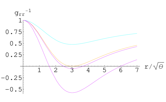
Figure 3: $g_{rr}^{-1}$ vs $r$, for various values of $M/\sqrt{\theta}$. Intercepts on the horizontal axis give radii of the event horizons. $M=\sqrt{\theta}$, ( cyan curve ) no horizon; $M=1.9\,\sqrt{\theta}$, (yellow curve) one degenerate horizon $r_{0}\approx 3.0\,\sqrt{\theta}$, extremal black hole; $M=3\,\sqrt{\theta}$ (magenta curve) two horizons.

Let’s start our analysis from the presence of eventual event horizons. Since in our case, the equation $g_{00}\left(\,r_{H}\,\right)=0$ cannot be solved in closed form, one can numerically determine their radius by plotting $g_{00}$. Figure (3) shows that noncommutativity introduces a new behavior with respect to standard Schwarzschild black hole. Instead of a single event horizon, there are different possibilities: (a) two distinct horizons for $M>M_{0}$ (yellow curve); (b) one degenerate horizon in $r_{0}=3.0\times\sqrt{\theta}$, with $M=M_{0}=1.9\times(\sqrt{\theta})/G$ corresponding to cyan extremal black hole (cyan curve); (c) no horizon for $M<M_{0}$ (violet curve). In view of these results, there can be no black hole if the original mass is less than the minimal mass $M_{0}$. Furthermore, contrary to the usual case, there can be two horizons for large masses. By increasing $M$, i.e. for $M>>M_{0}$, the inner horizon shrinks to zero, while the outer one approaches the Schwarzschild value $r_{H}=2M$.

For what concerns the covariant conservation of $T^{\mu\nu}$, one finds that such requirement leads to

$$T^{\theta}{}_{\theta}\equiv\partial_{r}\left(\,rT^{r}{}_{r}\,\right)=-\rho_{\theta}\left(\,r\,\right)-r\,\partial_{r}\rho_{\theta}\left(\,r\,\right).$$ (81)

The emerging picture is that of a self-gravitating, droplet of anisotropic fluid of density $\rho_{\theta}$, radial pressure $p_{r}=-\rho_{\theta}$ and tangential pressure $p_{\perp}=-\rho_{\theta}-r\,\partial_{r}\rho_{\theta}\left(\,r\,\right)$. We are not dealing with a massive, structure-less point. Thus results reasonable that a non-vanishing radial pressure balances the inward gravitational pull, preventing the droplet to collapse into a matter point. This is the basic physical effect on matter caused by spacetime noncommutativity and the origin of all new physics at distance scale of order $\sqrt{\theta}$. Regarding the physical interpretation of the pressure, we underline that it does not correspond to the inward pressure of outer layers of matter on the core of a “star”, but to a totally different quantity of “quantum” nature. It is the outward push, which is conventionally defined to be negative, induced by noncommuting coordinate quantum fluctuations. In a simplified picture, such a quantum pressure is the relative of the cosmological constant in DeSitter universe. As a consistency check of this interpretation we are going to show that line element (80) is well described near the origin by a DeSitter geometry.

Let us now consider the black hole temperature $T_{H}\equiv\left(\,\frac{1}{4\pi}\,\frac{dg_{00}}{dr}\right)_{r=r_{H}}$:

$$T_{H}=\frac{1}{4\pi\,r_{H}}\left[\,1-\frac{r^{3}_{H}}{4\,\theta^{3/2}}\,\frac{e^{-r^{2}_{H}/4\theta}}{\gamma\left(\,3/2\ ;r^{2}_{H}/4\theta\right)}\,\right]$$ (82)

For large black holes, i.e. $r_{H}^{2}/4\theta>>1$, one recovers the standard result for the Hawking temperature $T_{H}=\frac{1}{4\pi\,r_{H}}$. At the initial state of radiation the black hole temperature increases while the horizon radius is decreasing. It is crucial to investigate what happens as $r_{H}\to\sqrt{\theta}$. In the standard ( commutative ) case $T_{H}$ diverges and this puts limit on the validity of the conventional description of Hawking radiation. Against this scenario, temperature (82) includes noncommutative effects which are relevant at distances comparable to $\sqrt{\theta}$. Behavior of the temperature $T_{H}$ as a function of the horizon radius is plotted in Fig.(4).

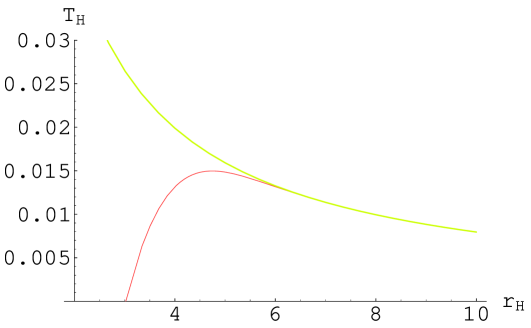
Figure 4: Plot of $T_{H}$ vs $r_{H}$, in $\sqrt{\theta}$ units. yellow curve is the plot of (82): $T_{H}=0$ for $r_{H}=r_{0}=3.0\sqrt{\theta}$,i.e. for the extremal black hole, while the maximum temperature $T_{H}\simeq 0.015\times 1/\sqrt{\theta}$ corresponds to a mass $M\simeq 2.4\times\sqrt{\theta}$. For comparison, we plotted in yellow the standard Hawking temperature. The two temperatures coincide for $r_{H}>6\,\sqrt{\theta}$.

In the region $r_{H}\simeq\sqrt{\theta}$, $T_{H}$ deviates from the standard hyperbola. Instead of exploding with shrinking $r_{H}$, $T_{H}$ reaches a maximum in $r_{H}\simeq 4.7\sqrt{\theta}$ corresponding to a mass $M\approx 2.4\,\sqrt{\theta}/G_{N}$, then quickly drops to zero for $r_{H}=r_{0}=3.0\sqrt{\theta}$ corresponding to the radius of the extremal black hole in figure (3). In the region $r<r_{0}$ there is no black hole and the corresponding temperature cannot be defined. As a summary of the results, the emerging picture of non commutative black hole is that for $M>>M_{0}$ the temperature is given by the Hawking temperature (0.45) with negligibly small exponential corrections, and increases, as the mass is radiated away. $T_{H}$ reaches a maximum value at $M=2.4\,\sqrt{\theta}$ and then drops as $M$ approaches $M_{0}$. When $M=M_{0}$, $T_{H}=0$, event horizon is degenerate, and we are left with a “frozen” extremal black hole.

At this point, important issue of Hawking radiation back-reaction should be discussed. In commutative case one expects relevant back-reaction effects during the terminal stage of evaporation because of huge increase of temperature swave ; backr . As it has been shown, the role of noncommutativity is to cool down the black hole in the final stage. As a consequence, there is a suppression of quantum back-reaction since the black hole emits less and less energy. Eventually, back-reaction may be important during the maximum temperature phase. In order to estimate its importance in this region, let us look at the thermal energy $E=T_{H}\simeq 0.015\,/\sqrt{\theta}$ and the total mass $M\simeq 2.4\,\sqrt{\theta}\,M_{Pl.}^{2}$. In order to have significant back-reaction effect $T_{H}^{Max}$ should be of the same order of magnitude as $M$. This condition leads to the estimate $\sqrt{\theta}\approx 0.2\,l_{Pl.}\sim 10^{-34}\,cm$. Expected values of $\sqrt{\theta}$ are well above the Planck length $l_{Pl.}$, while the back-reaction effects are suppressed even if $\sqrt{\theta}\approx 10\,l_{Pl.}$ and $T_{H}^{Max}\approx 10^{16}\,GeV$. For this reason we can safely use unmodified form of the metric (80) during all the evaporation process.

Finally, we would like to clarify what happens if the starting object has mass smaller than $M_{0}$, with particular attention to the eventual presence of a naked singularity. To this purpose we are going to study the curvature scalar near $r=0$. The short distance behavior of $R$ is given by

$$R\left(\,0\,\right)=\frac{4M}{\sqrt{\pi}\,\theta^{3/2}}$$ (83)

For $r<<\sqrt{\theta}$ the curvature is actually constant and positive. Thus, an eventual naked singularity is replaced by a DeSitter, regular geometry around the origin. Earlier attempts to avoid the curvature singularity at the origin of Schwarzschild metric have been made by matching DeSitter and Schwarzschild geometries both along time-like olds , and space-like matter shells dscore , or constructing regular black hole geometries by-hand regbh or continuosly deforming dilaton 2d models dejan . In our approach, it is noncommutativity that induces a smooth and continuous transition between the two geometries.

0.46 Concluding remarks

The above results show that the coordinate coherent state approach to noncommutative effects can cure the singularity problems at the terminal stage of black hole evaporation.

In particular we have shown that noncommutativity, being an intrinsic property of the manifold itself, can be introduced in General Relativity by modifying the matter source. The Energy-momentum required for this description is of form of the ideal fluid, although a non-trivial pressure is invoked. In spite of complicated equation of state it can be studied in the regions of interest and new black hole behavior is discovered in the region $r\simeq\sqrt{\theta}$. Specifically, we have shown that there is a minimal mass $M_{0}=1.9\,\sqrt{\theta}$ to which a black hole can decay through Hawking radiation. The reason why it does not end up into a naked singularity is due to the finiteness of the curvature at the origin. The everywhere regular geometry and the residual mass $M_{0}$ are both manifestations of the Gaussian delocalization of the source in the noncommutative spacetime. On the thermodynamic side, the same kind of regularization takes place eliminating the divergent behavior of Hawking temperature. As a consequence there is a maximum temperature that the black hole can reach before cooling down to absolute zero. As already anticipated in the introduction, noncommutativity regularizes divergent quantities in the final stage of black hole evaporation in the same way it cured UV infinities in noncommutative quantum field theory. We have also estimated that back-reaction does not modify the original metric in a significant manner.

Compactified Time and Likely Entropy — World Inside Time Machine: Closed Time-like CurvePreprints YITP-05-43; OIQP-05-09 H.B. Nielsen¹ and M. Ninomiya²Also at Okayama Institute for Quantum Physics, Kyoyama-cho 1-9, Okayama City 700-0015, Japan.

0.47 Introduction

In the present article we shall study a world or a (classical) mechanical system situated on a closed time-like loop, or we can simply consider a model of a universe intrinsically periodic. This is a study that can be considered a simple exercise playing with ideas that could be of relevance for making a (speculative) model behind the second law of thermodynamics MN1 MN2 MN3 MN3 MN4 .

One problem with combining the second law with time reversal symmetry, even if we hope for global features making $\dot{S}\geq 0$ in some era, is that then there is nothing prevent that in an other era – it is at least logically possible – we then have $\dot{S}\leq 0$. That in turn means that there are some restrictions known not only about the past but also about the future. Such rules about the future will function in a sense as time machine MN5 .

At least we can defend that there is the possibility of “time machine effects” in a model with such regularities about the future – regularities known from a mysterious, presumably not valid law of nature – in the sense that one could obtain what we should accept as messages from the future. We could ask: Why is it that we normally do not get messages from the future ?

Indeed the point is that a tiny amount of information from or about the past can allow us to make great deductions about the past because the past, which had low entropy, is very ordered. So from a little knowledge we can deduce a lot. Concerning the future on the other hand we cannot analogously trust the regularities. So even if we know a tiny amount of photons, say to develop into the future we cannot count on that they shall be involved with matter. They can just remain all through the future without getting associated with any other matters in the future. We cannot get messages from the future because we normally cannot conclude by use of regularity knowledge about the future from a tiny amount of information. For that the future can too easily be irregular. In our usual world picture (based on second law we might say) there is no regularity in the future except for the rudiments of regularity left over from the past. Therefore we cannot conclude anything great about the future from tiny informations like a little bit of light going into future. Even if we come to know that such a little bit of light runs into the future we do not accept that as a message from the future, because we cannot use that to make further significant deductions about the future. When we, however, get a letter or a fax, sent in the past we can use its content to conclude a lot about the past with reasonable reliability.

We want to stress that it is our knowledge about a relatively huge regularity in the past that makes it possible for us to consider small letters or light beams from the past as messages.

If however in some strange violation of the strict second law we came to know some regularity about the future, then we could begin to accept small pieces of light or paper with text on to give us messages about the future. We would then conclude that they would have to go into that pattern of regularities, which we had come to know as law of nature. If we for instance knew that there in some future should exist some very separate rather small hot places (time inverted stars) that would be more and more hot by absorbing light, then knowing that some light goes out in a certain direction will imply such time inverted star(s) in that direction. Then we could claim it were a message about such a time inverted star.

In any case we argue that because of the conflict between time reversal invariance and the second law, we can hardly imagine any spontaneous breakdown model behind second law providing us with say on era with $\dot{S}\geq 0$ unless we also have at least the possibility for also messages going the opposite way in time. So really models that could even have the slightest chance of a $T$-invariant model behind second law should have at least time machine effect elements in them.

It is therefore reasonable to exercise with as simple as possible models with such time machine effect elements in them. One of the simplest model of this sort for which there can be given several suggestive arguments is a world or the mechanical system of the model put on a closed time like curve (CTC). It shall turn out that this model indeed does only a very poor job with respect to being a model behind the second law of thermodynamics in as far as we shall end up with the conclusion that in such a closed loop time world the entropy is almost certainly totally constant, all around the time loop.

Such a time loop model can most simply be taken to mean that we postulate the set of moments of time to form an $S^{1}$-circle rather than a straight line (or some interval or half time axis in Big Bang theories). We can simply take it that the general relativity time coordinate is of such a nature that going forward in it by a certain constant $T$ (of dimension of time) we come by the coordinate map identifications to the same time moment (or say space-time points) as we started from. We could call this restriction that the world has got an intrinsic period $T$.

In the usual Big Bang picture which is in simple general relativity enforced by the knowledge of the Hubble expansion and suggestive phenomenology according to Hawking-Penrose’ singularity theorem such an intrinsic periodicity is of course not possible.

Nevertheless it might be imagined that in a final theory behind general relativity and not quite in agreement with the presuppositions of the just mentioned Big Bang enforcing theorem, it could e.g. happen that no start or crunch singularities were allowed.

In fact for instance superstring theory is presumably of the type without a starting point of time. There is possibility that a time parameter would go from $-\infty$ to $+\infty$, but it would still mean, in a sense, some singularities. Therefore the most elegant would be a compactified time.

Whatever there might be of essential reasons for even nature represented by a compact time or space-time manifold it is the purpose of the present article to study a world with closed timelike loops – really with a global forming closed loop – and compactified in space. As a matter of fact, however, we intend to consider so abstract formulation that we replace all the fields and their conjugates over the whole spatial extension of the compactified universe just by one (abstract) phase space. In other words we do not even consider space explicitly, but just a general mechanical system – i.e. a point moving in phase space according to a Hamilton’s equations –. The compactness of the time manifold $S^{1}$ then means that this general mechanical system is enforced to be strictly periodic with a period $T$ which is circumference of the above mentioned $S^{1}$.

Let us compare what we are concerned with a space-time with holographic principle MN6 . The holographic principle applies to worlds with a periodicity in time – and thus closed timelike loops – but still having a spatial infinity. Then what goes on in this space-time 4-volume is then determined by the boundary conditions at the spatial “far away”. This is holography in the sense that the information on the space-time field configurations packed into that on boundary surface placed far out in spatial direction.

In the present article we consider a compactified space so that there is no surface far out and then even the state of the system should be fixed alone by the structure of the system e.g. the Hamiltonian $H$ of the system if we think of it as the abstract mechanical system.

It is a very important point to have in mind for the present article that when time is compactified – it means in reality that a periodicity with given period is imposed – there are as many periodicity requirements as the dimension of the phase space. Also the manifold of initial conditions for the system has the same dimension since it simply $is$ the phase space. Unless some of the periodicity conditions are not independent or perhaps contradictory the expectation is that there are just a discrete set of solutions to enforced periodicity constraint. By considering a discrete set of solutions as “essentially” or “locally” just one solution we can say that the periodicity with enforced period $T$ fixes an “essentially” unique solution. When the Hamiltonian is not explicitly time dependent and thus conserved there is formally a one dimensional manifold of starting points, because a start at one of the points in phase space reached along the orbit of the system in phase space will just give rise to the same periodic motion just delayed in its development. But even that can be called an “essentially” unique solution. The main point is that compared to a phase space with a huge number of degrees of freedom some discrete solutions or even one dimensional sets of solutions is little different from a unique solution. By far most degrees of freedom get settled by the given period with periodicity fixing.

The main purpose of the present article is to deliver a very general estimate of what we would consider the entropy of the essentially unique solution as just stressed above, to our periodicity constraint with a fixed period. To put our estimate in perspective one should have in mind that if one chooses a random state of a mechanical system with a probability (density) given simply by the phase space measure, one almost certainly find it to have maximal entropy. The reason that it is so is because a macro state is associated with a volume of the phase space proportional to $e^{\frac{1}{k}S}$ where $k$ is the Boltzmann’s constant and $S$ the entropy. This is certainly true because the entropy $S$ could be defined to be $k\log$ (volume of phase space of macro state) MN7 .

With the above mentioned consideration in mind that thus the normal situation for a state chosen randomly in phase space is to have maximal entropy, it would be quite interesting to show that for a somewhat differently chosen state or point in phase space, the entropy is not maximal. This is indeed a remarkable thing.

The main point of the present article is precisely to show that with high probability the state obtained by the enforcement of the given period in advance for a “random system” will $not$ have maximal entropy.

In the following section 2 we set up a general formulation for macro states and approximately conserved quantities. In section 3 we argue for our expectations for the likely entropy of the state determined from enforced periodicity under some simplified assumptions. In section 4 we then take into account more general way of effective macro states without having them identified completely by sets of exactly conserved quantities. In section 5 we investigate the extension of our classical calculation of the likely entropy to quantum mechanics. In section 6 we conclude and present some outlook.

0.48 The philosophy of random Hamiltonian

It is the philosophy – as is usual – also in the present article to avoid fine tuning of any parameters, quantities involved in a given system. We can strengthen this by making the general assumption that apart from the symmetry restrictions which we impose the Hamiltonian and also other parameters or functions describing the model are taken to be random. This kind of randomness means that we e.g. for the Hamiltonian think of a probability distribution over the space of a large class of functions defined over phase space. That is to say that we have in mind a distribution density $P[H]$ destined to multiply a functional measure $\mathcal{D}H$ so that the probability for the Hamiltonian belonging to a certain subset ${\mathcal{A}}$ of “all” functions is given as

$$P_{\mathcal{A}}=\int_{\mathcal{A}}P[H]{\mathcal{D}}H~{}.$$ (84)

We may think of it this way, but in reality it is very difficult to find a reasonable functional integral measure $\mathcal{D}H$ so that not almost all functions after such a measure become very bad functions with respect to continuity and differentiability. For the purposes for which we want such random functions it is, however, not so important that the measure be precisely of such a form $P[H]\mathcal{D}H$. Thus we could as $\mathcal{D}H$ well instead take, some system of parameterized functions $H(\bm{\xi},\bm{q},\bm{p})$ depending on a set of parameters $\xi$.

Then we can choose – somewhat arbitrarily, but still in a reasonable way a measure over the space of parameters. By making the parameterization so that it guarantees smooth (continuously differentiable) functions we can in such a way obtain random differentiable functions. In as far as the Hamilton equations involve the partial derivatives of $H$ with respect to the $p_{i}$’s and the $q_{i}$’s it is of course strictly speaking needed that $H$ be differentiable. But in practice we care only for properties which are true “almost certainly” in the mathematical sense. In this way we mainly ignore null-sets (i.e. sets of functions with zero measure). The point of course is mainly that we do not accept our conclusions to be proven wrong by just a very specially made up counter-example. We could take the philosophy that it would be exceedingly strange if Nature should just have chosen a very special function. We really rather go for investigating what we shall typically expect. Really we believe that it is in a way a law of nature that unless we have some laws enforcing special feature we shall only get the most likely results according to such a randomness model. Really of course if we see something unlikely in this randomness philosophy we should make a new law explain so that it would no more be strange. That is how science works, you must make new laws whenever something is strange in the sense of violating the old ones or even just the statistical expectations derived using only the old laws.

The philosophy described in this section is essentially that of random dynamics, taking the laws of nature as random.

0.49 Setup of formalism for macro states

The formalism to make definition of entropy possible which we shall use here is of the following type: We imagine the phase-space of what we call the macro system divided up to a large number of “macro states” characterized by some “macroscopic variables”. That is to say we imagine some functions $\mathchoice{\mbox{\boldmath$\displaystyle\xi$}}{\mbox{\boldmath$\textstyle\xi$}}{\mbox{\boldmath$\scriptstyle\xi$}}{\mbox{\boldmath$\scriptscriptstyle\xi$}}(p,q)$ – called the “macroscopic variables” – to be defined over the phase-space the coordinates of which we denote symbolically as $(p,q)$. We then think of the set of all the points in phase space which within some finite small accuracy has given values $\mathchoice{\mbox{\boldmath$\displaystyle\xi$}}{\mbox{\boldmath$\textstyle\xi$}}{\mbox{\boldmath$\scriptstyle\xi$}}{\mbox{\boldmath$\scriptscriptstyle\xi$}}_{0}$ so that

$$\left|\mathchoice{\mbox{\boldmath$\displaystyle\xi$}}{\mbox{\boldmath$\textstyle\xi$}}{\mbox{\boldmath$\scriptstyle\xi$}}{\mbox{\boldmath$\scriptscriptstyle\xi$}}_{0}-\mathchoice{\mbox{\boldmath$\displaystyle\xi$}}{\mbox{\boldmath$\textstyle\xi$}}{\mbox{\boldmath$\scriptstyle\xi$}}{\mbox{\boldmath$\scriptscriptstyle\xi$}}(p,q)\right| < \varepsilon_{\rm macro},$$ (85)

as a macro state. Here $\varepsilon_{\rm macro}$ denotes a small quantity for the macroscopic variables. We can then define entropy $S(\mathchoice{\mbox{\boldmath$\displaystyle\xi$}}{\mbox{\boldmath$\textstyle\xi$}}{\mbox{\boldmath$\scriptstyle\xi$}}{\mbox{\boldmath$\scriptscriptstyle\xi$}}_{0}(\varepsilon))$ for the macro state at $\mathchoice{\mbox{\boldmath$\displaystyle\xi$}}{\mbox{\boldmath$\textstyle\xi$}}{\mbox{\boldmath$\scriptstyle\xi$}}{\mbox{\boldmath$\scriptscriptstyle\xi$}}(p,q)\approx\mathchoice{\mbox{\boldmath$\displaystyle\xi$}}{\mbox{\boldmath$\textstyle\xi$}}{\mbox{\boldmath$\scriptstyle\xi$}}{\mbox{\boldmath$\scriptscriptstyle\xi$}}_{0}$ as

$$S(\mathchoice{\mbox{\boldmath$\displaystyle\xi$}}{\mbox{\boldmath$\textstyle\xi$}}{\mbox{\boldmath$\scriptstyle\xi$}}{\mbox{\boldmath$\scriptscriptstyle\xi$}}_{0}(\varepsilon)) = k\log{\rm Vol}\left\{(p,q)\left||\mathchoice{\mbox{\boldmath$\displaystyle\xi$}}{\mbox{\boldmath$\textstyle\xi$}}{\mbox{\boldmath$\scriptstyle\xi$}}{\mbox{\boldmath$\scriptscriptstyle\xi$}}_{0}-\mathchoice{\mbox{\boldmath$\displaystyle\xi$}}{\mbox{\boldmath$\textstyle\xi$}}{\mbox{\boldmath$\scriptstyle\xi$}}{\mbox{\boldmath$\scriptscriptstyle\xi$}}(p,q)|\right.<\varepsilon_{\rm macro}\right\}$$ (86)

where $k$ denotes the Boltzmann constant.

Often in statistical mechanics one may meet macro states. However, the macro states appeared in the present paper may not quite seem to be of this kind. Thus it may be needed for us to define that it is in fact always allowed to work with our point of view.

Examples of the macro states which is not at first glance of the type we describe is made by almost all Gibbs ensembles and also by grand canonical ensembles. For a simple canonical ensemble one should think of the temperature as one of the macro state parameters i.e. one of the $\mathchoice{\mbox{\boldmath$\displaystyle\xi$}}{\mbox{\boldmath$\textstyle\xi$}}{\mbox{\boldmath$\scriptstyle\xi$}}{\mbox{\boldmath$\scriptscriptstyle\xi$}}_{0}$-components. Formally, all the states in canonical ensembles corresponding to two different temperatures $T_{1}$ and $T_{2}$ say are the same just with different probability (densities). Since it is well known that one can approximate for macroscopic systems by a canonical ensemble, we could make the temperature of a state in phase space $(p,q)$ be assigned as a function of the energy $H(p,q)$ for that state in phase space. The “temperature” $T(p,q)$ of the state $(p,q)$ should be made

$$T(p,q) = f(H(p,q))$$ (87)

where f is the function giving the macroscopic relation

$$T = f(U)$$ (88)

for the system. Here $U$ denotes the energy $U=\left<H\right>$.

Since the spread in energy $H$ for a canonical ensemble becomes rather small for highly macroscopic system the error by taking the entropy as we suggested above with $\varepsilon_{\rm macro}$ sufficiently big to allow the $H$-spread would be small.

It would be easy to argue similarly for grand canonical ensembles by approximating it by an ensemble with a fixed number of particles. Again we could use the approximately unique relation between the number of particles and the chemical potential and thus define a macroscopic variable among the $\mathchoice{\mbox{\boldmath$\displaystyle\xi$}}{\mbox{\boldmath$\textstyle\xi$}}{\mbox{\boldmath$\scriptstyle\xi$}}{\mbox{\boldmath$\scriptscriptstyle\xi$}}_{0}$’s to represent the chemical potential.

A priori it may be a question of our possibilities for finding some parameters which we can keep track of as our “macroscopic variables” $\textstyle\xi$. Such keeping track of the variables $\mathchoice{\mbox{\boldmath$\displaystyle\xi$}}{\mbox{\boldmath$\textstyle\xi$}}{\mbox{\boldmath$\scriptstyle\xi$}}{\mbox{\boldmath$\scriptscriptstyle\xi$}}(p,q)$ is the easiest if they are reasonably stable under the time development of the system. There will be total stability of the macroscopic variables $\mathchoice{\mbox{\boldmath$\displaystyle\xi$}}{\mbox{\boldmath$\textstyle\xi$}}{\mbox{\boldmath$\scriptstyle\xi$}}{\mbox{\boldmath$\scriptscriptstyle\xi$}}(p,q)$ if they are indeed conserved quantities such as changes. You could typically imagine that they would be taken to be conserved quantities such as angular momentum, linear momentum etc.

Since the possibility of choosing the macroscopic variables to be conserved quantities is such a simple way to ensure the stability of them we shall take this case as to be used in the next section. More generally, however, one may imagine a situation in which the macroscopic variables are not totally conserved but rather suffer some diffusion as time goes on.

0.50 The entropy estimate in the simple case of conserved macroscopic variables

Let us now illustrate the main argument for that the system with an enforced periodicity system will be in a state – or rather go through a series of states – in phase space not having maximal entropy. First we have, however, to specify in what sense we consider random systems or rather a system with a random dynamics. First of all it means that one imagines to put some probability measure over the set of all functions H defined on the phase space. Then one can assume that the Hamiltonian for the “random system” is obtained by picking a random Hamiltonian form H with a probability distribution given by the above mentioned probability measure.

To get an estimate of the probability for finding a periodic orbit with period $T$ beginning at $(q_{0},\rho_{0})$ we may think like the following: We imagine a system development by the Hamiltonian equations – using the random Hamiltonian H – which was started at $(q_{0},\rho_{0})$ at, say, $t=0$. As the Hamiltonian is “random” the development in time will be “random” too, except though for the selection rules or restrictions from that the macro variables are rather stable. In the simplest case of macro states characterized by (totally) conserved quantities $I_{i}$ say the system remains inside the subset of the phase space corresponding to the starting set of $I_{i}$-values. The volume in phase space of the subset to which the system started at $(q_{0},\rho_{0})$ is

$$u_{p}^{2N}\exp(S(\{I_{i0}\}))=u_{p}^{2N}\exp(S(\{I_{i}(q_{0},p_{0})\}))$$ (89)

where $S(\{I_{i}(q_{0},p_{0})\})$ is the entropy of the macro state – characterized by the conserved quantities $I_{i}=I_{i}(q_{0},p_{0})$ – corresponding to $(q_{0},p_{0})$, and $U_{p}$ is a factor inserted for each dimension to make the dimensionality correct without assigning the entropy very strange dimensionality. Thinking of defining $S$ by a quantum mechanical formula like (89) below we should take

$$u_{p}=\sqrt{h}$$ (90)

So the smaller this entropy $S(q_{0},p_{0})$ of the starting state $(q_{0},p_{0})$, so to speak, the smaller the volume to which the system of state will be confined.

Now the main thinking is that it is easier or more likely to reach back to the starting point $(q_{0},p_{0})$ by accident if the volume into which the system can move is smaller. Actually the probability to find back to the starting point $(q_{0},p_{0})$ just at time $t=T$ (where $T$ is the imposed period) within a given uncertainty range must be inversely proportional to the phase space volume which is $e^{S((q_{0},p_{0}))}$.

We could choose a certain fixes accuracy for which in the phase space by calling that practically we count all $(q,p)$ with

$$||(q,p)-(q_{0},p_{0})||^{2} < \varepsilon^{2}_{\rm p.s.}$$ (91)

as indistinguishable where $\varepsilon^{2}_{p.s.}$ denotes a chosen small accuracy error in phase space. For the purpose of judging if the period is just $T$, we accept $||(q_{0},p_{0})-(q(T),p(T))||^{2}<\varepsilon_{\rm p.s.}$ as the criterion for this periodicity condition. Here the $(q(T),p(T))$ are the time developed ones from $(q_{0},p_{0})$ during the time $T$. We may now simply estimate that the probability that $(q_{0},p_{0})$ with sufficient accuracy given by $\varepsilon_{\rm p.s.}$ gives rise to a periodic motion with period $T$ is

$$P\left((q_{0},p_{0})\mbox{ has }T\right)$$ (92)

$$= P\left[(q(T),p(T)),\mbox{ is inside $\varepsilon_{p.s.}$ sphere around }(q_{0},p_{0})\right]dq_{0}dp_{0}$$

$$\simeq Ce^{-S(q_{0},p_{0})}dq_{0}dp_{0}.$$

Here $dp_{0}dq_{0}$ is the (Liouville) phase space measure which is invariant under canonical transformations. The probability for finding a period $T$ starting point, i.e. a $(q_{0},p_{0})$ in a macro state (subset of phase space) with entropy $S({\rm macro}_{1})(=S(q_{0},p_{0}))$ is given by

$$C\int_{{\rm macro}_{1}}e^{-S(q_{0},p_{0})}dq_{0}dp_{0} = Ce^{S({\rm macro}_{1})}\times e^{-S({\rm macro}_{1})}$$ (93)

$$= C.$$

Thus all the possible macro states have the same probability for having a periodic orbit with period $T$.

This result is remarkable because the different macro states will typically have wildly different phase space volumes in as far as they are proportional to $e^{S({\rm macro})}$.

0.50.1 How is the realistic situation with respect to $T$-periodic orbits?

In this subsection we should estimate more realistically what the number of periodic orbits. In a macro state with $k$ fixed conserved quantities in a system with $N$ degrees of freedom so that phase space has dimension $2N$ this macro state has dimension $2N-k$. By use of integral invariants of Poincaré for small areas extending partly in the direction of a conserved quantity partly along its conjugate, we argue that small line pieces along these conjugate directions do neither extend nor contract as time goes on. This makes $k$ directions of zero scaling. The remaining $2N-2k$ dimension will typically scale up or down. Let us assume – we may still have to prove it – that half of them i.e. $N-k$ dimensions scale up while the rest of $N-k$ scales down. After long time a little region around $(q_{0},p_{0})$ will have scaled up exponentially with “Lyapunov exponents” (not only the maximal one, but all positive ones) and will have become enormous. The region obtained from the starting $2N-k$ very small region will be blown up to a huge $N-k$ dimensional surface, still with a bit of extension in the $k$ directions but strongly contracted in the $N-k$ directions of contraction.

We may imagine reaching such an approximately $N-k$ surface by propagating the very little region forward from $t=0$ to $t=\frac{T}{2}$. Similarly we should get an effectively $N-k$ dimensional one by propagating backward from $t=0$ to $t=-\frac{T}{2}$.

To seek periodic solutions for the system we should seek cuts of the two $N-k$ dimensional surfaces corresponding to $\frac{T}{2}$ and $-\frac{T}{2}$ respectively both surfaces lying in the $2N-k$ dimensional submanifold in phase space that represents the macro states characterized by the $k$ fixed conserved quantities ${I_{i}}$. they will generically never cut for given ${I_{i}}$’s because even to just cut in one point would require generically that the sum of the dimensions of the surfaces would become equal to the total dimension $2N-k$. Now $(N-k)+(N-k)=2N-2k$ and thus the $k$ parameters would have to be tuned to get a cutting. But $k$ is just the number of the dimensions of the space of the continuously many macro states and so we expect to find cutting for discrete values of the macro state characterizing conserved quantities ${I_{i}}$.

For the purpose of making an estimate of the number of solutions we should like to define an effective average of the Lyapunov exponent $\gamma_{av}$ so as to give the $(N-k)$ dimensional “area” of the $\frac{T}{2}$ surface defined above as

$$(\varepsilon_{\rm p.s.})^{N-k}\times\exp\left[\frac{T}{2}\cdot\gamma_{\rm av}\cdot(N-k)\right]$$ (94)

Here of course $\gamma_{\rm av}\leq\gamma$ where $\gamma$ is the maximal Lyapunov exponent. We must imagine, if we can consider in practice the macro state as compact, that the $N-k$ dimensional surfaces corresponding to $\frac{T}{2}$ and $-\frac{T}{2}$ are much folded back and forth and essentially cover the whole macro state. What we really want to estimate is the typical distances measured in the space of the different macro states i.e. in the space with the conserved variables $\{I_{i}\}$ as coordinates. We ask so to speak how large a $\Delta$ will give us just about one solution in the volume $\Delta^{k}$ in this space with extension $\Delta$.

If we call the distance we imagine to get out in the $\{I_{i}\}$ from the starting point $\Delta$ we cover a space of volume $\Delta^{k}$. After such extension we should get generic crossing and could ask how many crossings.

Let us define a “potential crossing volume” of dimension $2N-k$ and imbedded in the macro states as explained of this dimension as being the product of the three “areas”:

$$\varepsilon^{N-k}_{p,s}\exp(\frac{T}{2}\gamma_{av}(N-k))\cdot\varepsilon^{N-k}_{p,s}\exp(\frac{T}{2}\gamma_{av}(N-k))\cdot\Delta^{k}~{}.$$ (95)

The number of solution – in the $\Delta^{k}$ volume – is this $(2N-k)$-volume divided by the full volume of the phase

$$u^{2N-k}\exp(S)~{}.$$ (96)

Now above we though still did not sum over all the cells of size $\varepsilon^{2N-k}_{p,s}$ where the motion could have “started”. That of course should be in the phase in question having volume(96) (see page 19). So there is place for

$$\#~{}\mbox{cells}=\frac{u_{p}^{2N-k}}{\varepsilon_{p,s}^{2N-k}}\cdot\exp(S)$$ (97)

small cells.

However we do not really use the extension of the small cells in the direction of the $k$ dimensions corresponding to the conjugate variables to the conserved quantities, so it is better to think of only counting cells in the remaining $(2N-k)-k=2N-2k$ dimensions. We instead use the $\Delta^{k}$ volume to count for how far we should extend in the $\{I_{i}\}$-space to get the true crossing. But that then means that we should count the number of cells being for layers in the last $k$ dimensions out of the $2N-k$ but only in the $2N-2k$ ones corresponding to the dimensions in which we get the huge extension in one or the other time directions. In this point of view we should rather say that the number of cells we must use is

$$\#(\mbox{cells on surfaces}) = \frac{u_{s}^{2N-2k}}{\varepsilon_{p,s}^{2N-2k}}\exp\left(S\cdot\frac{2N-2k}{2N-k}\right)$$

$$= \left(\frac{u_{s}}{\varepsilon_{p,s}}\right)^{2N-2k}\exp\left(S\cdot\left(1-\frac{k}{2N-k}\right)\right)$$

$$\approx \left(\frac{u_{s}}{\varepsilon_{p,s}}\right)^{2N-2k}\cdot\exp(S)~{}.$$

Thus the full number of solutions is

$$\frac{\varepsilon_{p,s}^{N-k}\exp\left(\frac{T}{2}\gamma_{av}(N-k)\right)^{2}\Delta^{k}}{u_{s}^{2N-k}\exp(S)}\cdot\frac{u_{s}^{2N-2k}\exp(S)}{\varepsilon_{p,s}^{2N-2k}}~{}~{}.$$ (99)

In the light of the number of dimensions $k$ corresponding to the conserved quantities being tiny compared to the total number of degrees of freedom $N\gg k$ we do not consider the factor $\varepsilon_{p,s}^{-k}$ as very important. If therefore looks (at first) that the density of classical periodic solutions with just period $T$ is $\frac{1}{\Delta^{k}}$ evaluated so that there is just one solution per k-volume of order $\Delta^{k}$ which means so that

$$1\approx\varepsilon_{p,s}^{-k}\Delta^{k}\exp\left(T\gamma_{av}(N-k)\right)~{}~{}.$$ (100)

This density thus becomes

$$\frac{1}{\Delta^{k}}\approx\varepsilon_{p,s}^{-k}\exp\left(T\gamma_{av}(N-k)\right)~{}~{}.$$ (101)

At this stage it thus looks as if the density were wildly dependent on the average Lyapunov exponent through the presumably hugely varying factor

$$\exp\left(T\gamma_{av}(N-k)\right)~{}~{}.$$ (102)

This would indeed be the result if we took it that all the classical solutions had the same probability for being realized. But as we shall argue in the next subsection this is not realistic. Rather it will turn out that the bigger this huge factor is with the smaller weight should we count the solution in question so that actually this huge factor $\exp(T\gamma_{av}(N-k))$ gets (essentially) canceled and we end up with the result – again – that the density of probability in the space of macro states realized in the intrinsically periodic world is indeed very smooth, slowly varying compared to what huge variation that could have been imaged.

0.50.2 Weighting of the different classical solutions

In this subsection we include a correction in the sense that different classical solutions MN8 should not a priori be counted as equally likely but that these different tracks rather obtain a probability weight strongly related to the Lyapunov exponent.

Realistically we should always count that there is some uncertainty, even if small. If for no other reason, quantum mechanics will provide such a source of uncertainty. We shall though still postpone quantum mechanics proper to section 6 and it may be pedagogical here to think of some other source of uncertainty.

Let us here first develop – for self content – the behavior of orbits very close to a given classical solution by Taylor expanding the Hamiltonian say. Defining the deviations of the canonical coordinates $q_{i}$ and the conjugate momenta $p_{i}$ from their values $q_{cl~{}i}$, $p_{cl~{}i}$ along the considered classical motion

$$\Delta q_{i} = q_{i}-q_{cl~{}i}~{},$$ (103)

$$\Delta p_{i} = p_{i}-p_{cl~{}i}$$

we easily derive the Hamiltonian for the Hamilton equations for the deviations to the accuracy of up to second order terms in Taylor expansion

$$\Delta\dot{q}_{i} = \dot{q}_{i}-\dot{q}_{cl~{}i}$$ (104)

$$= \sum_{j}\frac{\partial^{2}H}{\partial q_{j}\partial p_{i}}\Delta q_{i}+\sum_{j}\frac{\partial^{2}H}{\partial p_{j}\partial p_{i}}\Delta p_{j}~{},$$

$$\Delta\dot{p}_{i} = -\sum_{j}\frac{\partial^{2}H}{\partial q_{j}\partial q_{i}}\Delta q_{j}-\sum_{j}\frac{\partial^{2}H}{\partial p_{j}\partial q_{i}}\Delta p_{j}~{}.$$

Equivalently in matrix form they read

$$\left(\begin{array}[]{c}\Delta\dot{q}_{1}\\ \Delta\dot{q}_{2}\\ \vdots\\ \Delta\dot{q}_{N}\\ \Delta\dot{p}_{1}\\ \Delta\dot{p}_{2}\\ \vdots\\ \Delta\dot{p}_{N}\\ \end{array}\right)=\underline{M}\left(\begin{array}[]{c}\Delta q_{1}\\ \Delta q_{2}\\ \vdots\\ \Delta q_{N}\\ \Delta p_{1}\\ \Delta p_{2}\\ \vdots\\ \Delta p_{N}\\ \end{array}\right)$$ (121)

where $\underline{M}$ is the $2N\times 2N$ matrix of second derivatives of the Hamiltonian

$$\underline{M}=\left(\begin{array}[]{cc}\frac{\partial^{2}H}{\partial q_{j}\partial p_{i}}&\frac{\partial^{2}H}{\partial p_{j}\partial p_{i}}\\ -\frac{\partial^{2}H}{\partial q_{j}\partial q_{i}}&-\frac{\partial^{2}H}{\partial p_{j}\partial q_{i}}\\ \end{array}\right)~{}~{}.$$ (124)

Here $N$ is the number of degrees of freedom and the four symbols $\frac{\partial^{2}H}{\partial q_{j}\partial q_{i}}$ etc. stand for the four $N\times N$ submatrices, with $i$ enumerating the rows and $j$ the columns.

Introducing the $2N\times 2N$ matrix

$$\underline{J}=\left(\begin{array}[]{cc}\underline{0}&\underline{1}\\ \underline{-1}&\underline{0}\\ \end{array}\right)$$ (127)

we note that the time development matrix $\underline{M}$ obeys

$$\underline{J}~{}\underline{M}~{}\underline{J}=\left(\begin{array}[]{cc}\frac{\partial^{2}H}{\partial p_{j}\partial q_{i}}&\frac{\partial^{2}H}{\partial q_{j}\partial q_{i}}\\ -\frac{\partial^{2}H}{\partial p_{j}\partial p_{i}}&-\frac{\partial^{2}H}{\partial q_{j}\partial p_{i}}\\ \end{array}\right)=\underline{M}^{T}~{}.$$ (130)

¿From this property we immediately obtain that the spectrum for frequencies $\omega$ defined from seeking deviations

$$\left(\begin{array}[]{c}\Delta q_{1}\\ \vdots\\ \Delta q_{N}\\ \Delta p_{1}\\ \vdots\\ \Delta p_{N}\\ \end{array}\right)=e^{-i\omega t}\left(\begin{array}[]{c}\Delta q_{1~{}0}\\ \vdots\\ \Delta q_{N~{}0}\\ \Delta p_{1~{}0}\\ \vdots\\ \Delta p_{N~{}0}\\ \end{array}\right)$$ (143)

with the $\Delta q_{i~{}0}$ and $\Delta p_{i~{}0}$’s being constant in time is defined as the eigenvalue spectrum for $\omega$ as

$$-i\omega\left(\begin{array}[]{c}\Delta q_{1~{}0}\\ \vdots\\ \Delta p_{N~{}0}\\ \end{array}\right)=\underline{M}\left(\begin{array}[]{c}\Delta q_{1~{}0}\\ \vdots\\ \Delta p_{N~{}0}\\ \end{array}\right)$$ (150)

or from the zeros of the secular equation

$$0=\mathcal{D}et(\underline{M}+i\omega\underline{1})$$ (151)

from where it is seen to consist of pairs of opposite eigenvalues. That is to say if $\omega$ is an eigenvalue then so is also $-\omega$. In fact equation (151) implies

$$0 = \mathcal{D}et(\underline{M}^{T}+i\omega\underline{1})=\mathcal{D}et(\underline{J}~{}\underline{M}~{}\underline{J}+i\omega\underline{1})$$

$$= \mathcal{D}et(\underline{-M}+i\omega\underline{1})\Rightarrow\mathcal{D}et(\underline{M}-i\omega\underline{1})$$

and so we see that together with $\omega$ we must also have $-\omega^{*}$ as an eigenfrequency, namely by complex conjugating equation (150) which gives that the complex conjugate column $\left(\begin{array}[]{c}\Delta q^{*}_{1~{}0}\\ \vdots\\ \Delta p^{*}_{N~{}0}\\ \end{array}\right)$ is an eigenvector corresponding to the frequency $-\omega^{*}$. Provided we do not have a whole set of four different related eigenvalues $(\omega,-\omega,-\omega^{*},\omega^{*})$ but rather only two related eigenvalues we must have either

$$-\omega^{*}=\omega~{}~{}~{}\mbox{or}~{}~{}-\omega^{*}=-\omega~{}.$$ (153)

The possibility (153) only allows that $\omega$ is either purely imaginary or purely real. Both these possibilities are easily seen to be indeed realizable respectively the inverted and usual harmonic oscillator used as examples.

In the case of $\omega$ real the paths close to a given classical solution circle around the latter, much like a harmonic oscillator – or rather several – in phase space circles around the equilibrium point. If we however have the purely imaginary $\omega=-\omega^{*}$ then the situation is rather analogous to “the inverted harmonic oscillator”, meaning a particles near the top of a hill. In such an unstable equilibrium situation it is well known that the solutions are rather of the form of linear combinations of exponentially varying solutions in time of the form $e^{\pm\gamma t}$ call the coefficients in the exponent, $\gamma=Im~{}\omega$, in time local Lyapunov exponents. In any case it is very important for the cancellation, which we are going to show that averaging over time these eigenvalues $\pm\gamma$ are closely related to our averaged Lyapunov exponent $\gamma_{av}$. In fact we have the relation

$$\int_{\mbox{the period $T$ along the classical path}}\sum_{\mbox{the different eigenvalues}}|\gamma(t)|dt\frac{1}{T}=\gamma_{av}~{}.$$

(154)

In principle $\gamma_{av}$ depends on the path.

The physical meaning of these imaginary frequencies $\omega=i\gamma$ is that the nearby paths soon move away from the given classical path $(q_{i~{}0}(t),p_{i~{}0}(t))$ exponentially. If we thus put some cut off – some accuracy of measurement say – for how far out we still consider a neighboring path connected with the given classical path still in the neighbourhood, this border will be crossed every unit of time by the fraction of all the surrounding neighbouring paths being

$$\mbox{``Fraction being lost per unit time"}=\sum_{|\gamma|}|\gamma(t)|~{}.$$ (155)

Note that the probability for some random neighboring path is all the time given by (155) independent of the precise size and shape of the cut off chosen to define whether a path is still in the (closed) neighbourhood. It is only required that the cut off is chosen to give a small enough neighborhood that the Taylor expansion we used is valid as a good approximation. That we have this loss rate (155) independent of the details of the cut off is of course a consequence of the spreading of the neighboring track/paths is a pure (exponential) scaling up with time, a scale invariant operation (i.e. not involving any unit for say $q_{i}$).

When we now consider a classical periodic path with intrinsic period $T$, we should realistically think of it as representing a tiny little neighborhood of accompanying paths. Now following along the classical path we have just calculated the loss rate of these accompanying path. That means that whatever neighborhood we had chosen to represent the “accompanying paths” we loose per unit time the fraction $\sum_{|\gamma|}|\gamma(t)|$ of them. So the total fraction of the accompanying tracks which survive all the period $T$ through is

$$\mbox{``Surviving fraction"}=\exp\left(-\int_{\mbox{along the period}}\sum_{|\gamma|}|\gamma(t)|dt\right)~{}.$$ (156)

This is actually the “average Lyapunov”.

$$\mbox{``Surviving fraction"}=\exp\left(-\gamma_{av}(\mbox{for the cl. solution)}T\right)~{}.$$ (157)

It is obvious that starting with a random start very close to one of the periodic solutions the chance that it will return a period later equally very close is only this $``survivalfraction"=\exp\left(-\gamma_{av}(\mbox{for the track)}T\right)$. We should therefore not take all the classical periodic solutions with period $T$ as equally likely, but rather we should weight them statistically with weight factor $\exp\left(-\gamma_{av}(\mbox{for the solution)}T\right)$.

Interestingly enough this probability weight which a priori could have influenced the relative likelihood for different macro states, happens to just cancel the corresponding factor $\exp(\gamma_{av}T)$ occurring in the number of solutions. That is to say: the effect of loosing the accompanying path due to the spreading intervals in time where some period $\omega$ are imaginary is just compensated by the way the number of solutions is also sensitive to the Lyapunov exponents.

So we really do not need to calculate Lyapunov exponents to estimate the likelihood of the various macro states in our intrinsic periodicity model. The result that all the macro states have similar probability for being realized in the model is still true even when the Lyapunov exponents were taken into account because their effect is remarkably just canceled out!

0.51 More general macro states

If one makes the assumption used in foregoing section that the macro states are totally specified by a series ${I_{i}}$ of conserved quantum numbers $I_{i}$, then the macro state cannot change with time at all. Thus entropy variation with time is completely excluded under such conditions. Thus any hope of deriving the second law of thermodynamics in such a model would be excluded alone for the reason that the macro state could not change.

We therefore must make the assumptions a little more liberal so that the macro states are able to change the one into the other one. These processes of changing macro state should still be somewhat suppressed and unlikely. Nevertheless it should now be possible.

We wish to argue, however, by an argument similar to that of section 3 that it is unlikely that the periodic orbit with given period T will have its entropy change, but very little. Hereby we mean that the macro state – if it changes at all – will only change between macro states with approximately the same entropy.

The argument runs indeed in the following way: we ask for the probability of a motion of the system starting at a phase space point $(q_{0},p_{0})$ with sufficient accuracy periodic with the period $T$. Let us say that $(q_{0},p_{0})$ belongs to a macro state $(q_{0},p_{0})_{M}$ with entropy $S((q_{0},p_{0})_{M})$ where M denotes macro states, but that during the motion with time $t$ the system runs into other macro states $M_{1},M_{2}$, etc.. The chance for the system to be at time $t=T$ (by assuming to at $t=0$) back again at $(q_{0},p_{0})$ is inversely proportional to $\sum_{i}e^{S(M_{i})}\approx e^{\max S(M_{i})}$. That is to say that it is inversely proportional to the exponentiated entropy for that of the passed macro states, which has the biggest entropy,

$$\max\left\{S(M_{i})\;|\;i\mbox{ corresponding the passed }M\right\}$$ . (158)

But the phase space for a starting point $(q_{0},p_{0})$ in a macro state $M_{k}$ is $e^{S(M_{k})}=e^{S(q_{0},p_{0})}$. Thus the chance goes as

$$e^{S(q_{0},p_{0})-\max\left\{S(M_{i})\right\}} \leq 1.$$ (159)

By having the entropy vary during the periodic motion will – always – bring down the relative probability, in fact by the factor given by the left hand side of (159). In this way it gets more and more unlikely the bigger the spread in the entropy during the passage.

Ignoring the small variation in entropy allowed and it is indeed only a very small amount allowed, we conclude that the entropy will stay constant.

In the above statement we argued completely generally and in an abstract manner with the compactified time manifold of the form $S^{1}$ that the initial conditions become essentially fixed and that in such a way that the entropy becomes completely conserved. Note that this means that in such a machinery – which can be said exists inside a time machine, i.e. closed time like loop – the entropy becomes constant and there would be no place for a nontrivial entropy increase. Therefore the second law of thermodynamics would only be true in the trivial manner that entropy stands still. A nontrivial increase would not be allowed.

Logically it thus seems that since we have certainly the nontrivial increase in nature we would have to claim that the world would not possibly turn out to be of type of the compactified time as discussed in this article.

It could be greatly interesting to remark that as superstring theory is said to be of the type without the singularities initiating or finalizing the time-axis, then our way of arguing would imply that superstring theory would not be compatible with second law of thermodynamics.

We must, however, admit the caveat that our phase space were taken in the discussion as of finite volume. Thus if the “system” were a field theory in an infinite space, then perhaps we should reconsider the argument. Arrow of time axis turn out to infinity could spoil this argument.

0.52 Attempt to extend to quantum mechanics

At first one would have thought that the argument in section 3 that enforcing periodicity with the period $T$ would lead to essentially all macro states having equal probability, should easily be extended to work also for quantum mechanical systems. However, strangely enough we shall see that at first it does not extend to quantum mechanics.

To repeat the same story quantum mechanically, in the simplest case we should consider a quantum mechanical system with a series of conserved operators $I_{i}$ – among which $I_{i}$ is the Hamiltonian – get that the imposed periodicity $T$ simply comes to require that

$$TH = TI_{1}^{\prime}\ =\ 2\pi n,$$ (160)

and $I_{1}^{\prime}$ the eigenvalue of $I_{1}=H$ with an integer $n$. In this way all the states defined by

$$\left\{\left|\psi\right>\left|\;\forall i\;[\hat{I}_{i}\left|\psi\right>=I_{i}^{\prime}\left|\psi\right>]\right.\right\}$$ (161)

will be unchanged by the time development operator $e^{-iTH}$ for the period $T$. If we now ask for the macro state specified to have the subspace characterized by a set of eigenvalues ${I_{i}}$ the allowed set consists of the set of macro states that satisfy eq (160). The dimension of this subspace is obviously to be identified with $e^{S(M)}$ where $S(M)$ is the entropy of the macro state $M$. Here the entropy is given by

$$S(\{I_{i}\}) = \log\dim\left\{\left|\psi\right>\left|\;\forall i\;(\hat{I}_{i}\left|\psi\right>=I_{i}^{\prime}\left|\psi\right>)\right.\right\}~{}.$$ (162)

Taking seriously that Hamiltonian $H=I_{1}$, say, is among macro state specifying parameters, we simply get the condition for the periodic system with period $T$ as

$$TH^{\prime} = TI_{1}^{\prime}\ =\ 2\pi n$$ (163)

with an integer $n$. It means that the time translation operator through the micro states in the macro states in question. Actually it is obvious that on the states in eq (161), the time translation operator acts as

$$e^{-iTH}\left|\psi\right> = \left|\psi\right>.$$ (164)

This simple relation means that the macro states with the imposed period $T^{\prime}$ are just those with a series of $I_{1}^{\prime}$ values of multiple of $\frac{2\pi}{T}$. Such macro states be with a smooth distribution in the space of $\{I_{i}^{\prime}\}$ values. In this manner we reached a result similar to the one in section 3. The entropy can vary a lot as the $\{I_{i}^{\prime}\}$ values are varied and thus we still have the surprise that we get smooth probability distribution in the manifold of macro state in spite of the strong variation in entropy $S$ and therefore huge variation of the phase space volume $e^{S}$.

0.53 Conclusion and outlook

We have studied the consequences of imposing a given period $T$ in advance on a “random” physical system. What we found were that such a condition is in general only fulfilled for some or few macro states. The remarkable point is that this macro state is not simply one with maximal entropy. On the contrary we rather get for a random system same probability for the different macro states to contain a macro state obeying the periodicity $T$ requirement.

We got this result both quantum mechanically and classically. It should be stressed that our quantum mechanical result came by using the Hamiltonian as one of our macroscopic variables. It should be born in mind that such a world that has an imposed fixed period $T$ is a world which can be said to exist inside a time machine. Actually it is obvious that an enforced periodic time variable running on $S^{1}$ means a time machine in the sense that one gets back in time by the periodicity which simply brings a person – part of the system we consider – which lives into time $T$ back to time $0$. As a consequence of the world considered – containing in a time machine, it expected to have “grand mother paradoxes” which have to be resolved by some miracles. We can consider the surprisingly low entropy resulting for a random model of the type of the fixed period as an expression of the “miraculous” solution to the inconsistencies otherwise easily popping up.

An outlook to an application of the present work could be that we suppose that for some reason or another – philosophically that there be no singularities at which time stops or begins, or superstring theory – the time manifold is forced to be compact and thus we are forced to a periodic world development. Then this world would have a promising point concerning the establishment of a “deeper understanding” of the second law of thermodynamics. However, to get a varying entropy with time is seemingly not coming, so really it was not a successful model to explain second law of thermodynamics.

We seek to present our failure to obtain in such a model the genuine increase of entropy into a no-go theorem developing the rather trivial point that second law is strictly speaking in disagreement with the time reversal symmetry principle: The well known arrow of time problem MN9 . Could even some time reversal invariant laws allow naturally say in time locally in some era, an effective second law to be valid. We hope in near future to see which conditions are enough to make even such models impossible.

Astri Kleppe’s Song

Wolf light

I

You asked me in my dream
what time is. When I answered you turned
away
But I know, I called out
and knew
Already was my answer dissolved

Where does the recent now
of a moment pass? My face
you just saw,
”imagine that the world emerged by a mistake,
like when you lose a plexiglass
on a stone floor”

II

I have a picture of you
on the wall, black, white
and grey

March twilight, an airplane shadow
moves over the roofs
What is it the paper attempts to
interpret? The granularity
of the pigmentation effaces the angles
of your eyes, and the mouth keeps moving
under my effort to see. What
is an other? Air planes
plunged in borrowed light,

on summer mornings, a little child
who plays by the seashore (the colours of stones are clearer in water),
and the stone which is me
is washed over
by other rains, by the prospects
of other truths
Three straight cuts, a giant
crosses over. And under the roofs
the street space catches hold
of the slowly wandering
of nearby stars
Like us, perhaps they call their neighbours
But which homes, which places
in this sinking?

III

It is quiet. I breathe and it is silent,
we talked at length and I shut my eyes, lifted
by pictures gently passing,
the oddness of a touch
of other seashores

It is quiet. Am I asleep?
We talked a minute ago about the burned land,
the meadow’s faithless green. It retains
no steps, Earth’s file of index cards
where exchangeable pass
Maybe in the glimpses between sleep and wake,
the waves between dead and alive,

like the sun ray forcing
its way through the heavy curtain, a way
through the room, in the hair
on her shoulders, in the stripes
of her lips. She looks up, somehow
astonished

Scent of linen, charlock blossom,
an afternoon wind drives across the field
And she dips her fingers
in the water furrows,
perhaps the dead communicate
by means of winds, of wind grey
aspens

IV

I was a child
by the water side, played
with the shells
and stones, wrinkles
of sand
Sometimes we collected mussels
But no fire

Like stars, stones dispersed,
glittering in the sun. According to which
order are they given room, which clockwork
carries stones, the movement of stars?
Voids fumbling
in each other’s space, clamping
onto nothing, falling
towards nothing

No, why should anyone
be more concerned
than the sun by a water surface,

than a feather by the waves, so light
And groping for another Earth, attachments
for the weightiness. They said affinities
draw limitations through all
things, specific ones
for every body

V

”Every man has a part in light”, on my wall
I have a picture. Of you? These eyes that look at me
so questioning, accusingly
O, let us chat, let us tell some lies
together
Breakfast light, let us wake up, perhaps
we talk about our dreams, a door
that can’t be opened and something
that approaches, weird
and other

The snow light is so white today
I dreamt we walked
along the road, a winter day like now
Then suddenly I saw the buds, all swelling
like in May

The rooms are much too white
You said you are a stranger here, but trees
are they not just as strange? Indifferent
their frozen time which flows away
I looked out of a window
in my dream. A yard
there under me, enclosure
with a tree
From which a piece of cloth is hanging, and I strech out
to reach it as it flutters back, around
the tree and drapes it

And in the dream you tell me
that to carry fruit the tree
invokes the darkness
where all light is hidden

VI

The Milky Way hovers
in dimmer light,
for skaters’ moist dance, a city

where fragments of nightly tales
appear. They sang
you must tar your back
and keep fir twigs
in mind, sign secret weeping,
weep and tar

And space grows denser there,
your face,
your ears spread out, a
picture’s hunger
Thursday, vacuum-cleaning, laundry,
and the witch goes to the
supermarket, gets
her dough for gingersnaps
and eggs and matches, tsimtsum, in this
best of worlds, laboratory
for Paradise studies

And sure, we have mapped out
the trajectories of motion, and you
fried eggs for breakfast, they should be eaten there
at once

you said, and morning
struck into the kitchen,
pictureless like time,
and lemon green

VII

On my wall
I have a portrait
Reflected in the wall stains,
in shadows long since erased

”They have taken my face
away from me”,
wrinkles between gold foils, pictures
of time, all time, clay eyes
out of the dusting earth
where the young child plays in the early light

…perhaps she covered her ears afterwards,
when she had ignited
(that was the fire)

 

Blejske Delavnice Iz Fizike,   Letnik 6, št. 2,     ISSN 1580–4992

Bled Workshops in Physics,    Vol. 6, No. 2

Zbornik 8. delavnice ‘What Comes Beyond the Standard Models’, Bled, 19. – 29. julij 2005

Proceedings to the 8th workshop ’What Comes Beyond the Standard Models’, Bled, July 19.–29., 2005

Uredili Norma Mankoč Borštnik, Holger Bech Nielsen, Colin D. Froggatt in Dragan Lukman

Publikacijo sofinancira Javna agencija za raziskovalno dejavnost Republike Slovenije

Tehnični urednik Vladimir Bensa

Založilo: DMFA – založništvo, Jadranska 19, 1000 Ljubljana, Slovenija

Natisnila Tiskarna MIGRAF v nakladi 100 izvodov

Publikacija DMFA številka 1618

References

- (1) E.W. Kolb and M.S. Turner, The Early Universe, Addison-Wesley Pub. Co. 1989
- (2) D. Bennett and H.B. Nielsen, Int. J. of Mod. Phys. A9 (1994) 5155 ,
- (3) D. Bennett and H.B. Nielsen, Int. J. of Mod. Phys. A14 (1999) 3313,
- (4) C.D. Froggatt and H.B. Nielsen, Phys. Lett. B368 (1996) 96.

References

- (1) For a recent review and an extensive list of references, see: S. Carlip, Conformal Field Theory, (2+1)-Dimensional Gravity, and the BTZ Black Hole, preprint gr-qc/0503022.
- (2) J. D. Brown and M. Henneaux, Comm. Math. Phys. 104 (1986) 207.
- (3) E. Witten, Nucl. Phys. B311 (1988) 46; A. Achucarro and P. Townsend, Phys. Lett. B180 (1986) 89.
- (4) M. Bañados, C. Teitelboim and J. Zanelli, Phys. Rev. Lett. 16 (1993) 1849; M. Bañados, M. Henneaux, C. Teitelboim and J. Zanelli, Phys. Rev. D48 (1993) 1506.
- (5) See, for instance: M. Bañados, Phys. Rev. D52 (1996) 5861; A. Strominger, JHEP 9802 (1998) 009; M. Bañados, Three-dimensional quantum geometry and black holes, preprint hep-th/9901148; M. Bañados, AIP Conf. Proc. No. 490 (AIP, Melville, 1999), p. 198; M. Bañados, T. Brotz and M. Ortiz, Nucl. Phys. B545 (1999) 340.
- (6) See, for instance: M. Blagojević, Gravitation and gauge symmetries (Institute of Physics Publishing, Bristol, 2002); Three lectures on Poincaré gauge theory, SFIN A1 (2003) 147, preprint gr-qc/0302040.
- (7) E. W. Mielke, P. Baekler, Phys. Lett. A156 (1991) 399. P. Baekler, E. W. Mielke, F. W. Hehl, Nuovo Cim. B107 (1992) 91.
- (8) A. García, F. W. Hehl, C. Heinecke and A. Macías, Phys. Rev. D67 (2003) 124016.
- (9) M. Blagojević and M. Vasilić, Phys. Rev. D67 (2003) 084032; Phys. Rev. D68 (2003) 104023; Phys. Rev. D68 (2003) 124007.
- (10) M. Blagojević and B. Cvetković, Canonical structure of 3d gravity with torsion, preprint gr-qc/0412134.
- (11) S. Cacciatori, M. Caldarelli, A. Giacommini, D. Klemm and D. Mansi, Chern-Simons formulation of three-dimensional gravity with torsion and nonmetricity, preprint hep-th/0507200.
- (12) M. Blagojević and B. Cvetković, Black hole entropy in 3d gravity with torsion, in preparation.

References

- (1) N. S. Mankoč Borštnik,“Spin connection as a superpartner of a vielbein” Phys. Lett. B 292, 25-29 (1992).
- (2) N. S. Mankoč Borštnik, “Spinor and vector representations in four dimensional Grassmann space”, J. Math. Phys. 34, 3731-3745 (1993).
- (3) N. Mankoč Borštnik, ”Poincaré algebra in ordinary and Grassmann space and supersymmetry”, J. Math. Phys. 36, 1593-1601(1994),
- (4) N. S. Mankoč Borštnik, ”Unification of spins and charegs in Grassmann space?”, Modern Phys. Lett. A 10, 587-595 (1995),
- (5) N. S. Mankoč Borštnik and S. Fajfer, ”Spins and charges, the algebra and subalgebra of the group SO(1,14) and Grassmann space, N. Cimento 112B, 1637-1665(1997).
- (6) A. Borštnik, N. S. Mankoč Borštnik, “Are Spins and Charges Unified? How Can One Otherwise Understand Connection Between Handedness (Spin) and Weak Charge?”, Proceedings to the International Workshop on “What Comes Beyond the Standard Model, Bled, Slovenia, 29 June-9 July 1998, Ed. by N. Mankoč Borštnik, H. B. Nielsen, C. Froggatt, DMFA Založništvo 1999, p.52-57, hep-ph/9905357.
- (7) N. S. Mankoč Borštnik, H. B. Nielsen, ”Dirac-Kähler approach conneceted to quantum mechanics in Grassmann space”, Phys. Rev. 62 (04010-14) (2000),
- (8) N. S. Mankoč Borštnik, “Unification of spins and charges”, Int. J. Theor. Phys. 40, 315-337 (2001) and references therein.
- (9) A. Borštnik, N. S. Mankoč Borštnik, “Weyl spinor of SO(1,13), families of spinors of the Standard model and their masses”, Proceedings to the International Workshop on “What Comes Beyond the Standard Model”, Bled 2000,2001,2002 Volume 2, Ed. by N. Mankoč Borštnik, H. B. Nielsen, C. Froggatt, Dragan Lukman, DMFA Založništvo 2002, p.27-51, hep-ph/0301029, and the paper in preparation.
- (10) A. Borštnik, N. S. Mankoč Borštnik, “The approach unifying spins and charges in and its predictions”, Proceedings to the Euroconference on Symmetries Beyond the Standard Model, Portorož, July 12-17, 2003, Ed. by N. Mankoč Borštnik, H. B. Nielsen, C. Froggatt, Dragan Lukman, DMFA Založništvo 2003, p.27-51, hep-ph/0401043, hep-ph/0401055, hep-ph/0301029.
- (11) E. Witten, Nucl. Phys. B 186 412 (1981); Princeton Technical Rep. PRINT -83-1056, October 1983.
- (12) M. Blagojević, Gravitation and gauge symmetries (I. of Phys. Pub, ISBN 0750307676, 2001).
- (13) N. S. Mankoč Borštnik, H. B. Nielsen, hep-th/0509101.
- (14) A.Borštnik Bračič, N. S. Mankoč Borštnik, ”On the origin of families and their masses”, hep-ph/05
- (15) N. S. Mankoč Borštnik, H. B. Nielsen, “How to generate spinor representations in any dimension in terms of projection operators, J. of Math. Phys. 43, 5782-5803, hep-th/0111257.
- (16) N. S. Mankoč Borštnik, H. B. Nielsen, “How to generate families of spinors”, J. of Math. Phys. 44 (2003) 4817-4827, hep-th/0303224.
- (17) N. S. Mankoč Borštnik, H.B. Nielsen, ”Coupling constant unification in spin charge unifying model agreeing with proton decay measurments”, Proceedings to the Workshop ”What Comes Beyond the Standard Models”, Bled, 2000,2001,2002, Ed. by N. Mankoč Borštnik, H. B. Nielsen, C. Froggatt, Dragan Lukman, DMFA Založništvo 2002, p.94-105, hep-ph/0301029.
- (18) N. S. Mankoč Borštnik, H. B. Nielsen, “Coupling constant unification in spin-charge unifying model agreeing with proton decay measurement“, in preparation.
- (19) H. Georgi Lie algebras in particle physics (The Benjamin/cummings, London 1982).
- (20) V.A. Novikov, L.B. Okun,A.N. Royanov, M.I. Vysotsky, “Extra generations and discrepancies of electroweak precision data”, hep-ph/0111028.
- (21) A. Kleppe, D. Lukman, N.S. Mankoč Borštnik, ”About families of quarks and leptons”, Proceedings to the Workshop ”What Comes Beyond the Standard Models”, Bled, 2000,2001,2002, Ed. by N. Mankoč Borštnik, H. B. Nielsen, C. Froggatt, Dragan Lukman, DMFA Založništvo 2002, p.94-105, hep-ph/0301029.
- (22) M.Breskvar, J. Mravlje, N.S. Mankoč Borštnik, ”Prediction for Four Generations of Quarks and Leptons Suggested by the Approach Unifying Spins and Charges”, Proceedings to the Workshop ”What Comes Beyond the Standard Models”, Bled, July 19-31, 2004, Ed. by N. Mankoč Borštnik, H. B. Nielsen, C. Froggatt, Dragan Lukman, DMFA Založništvo 2004, p.1-16, hep-ph/0412208.
- (23) H. Fritsch, Phys. Lett.73 B,317 (1978).
- (24) S. Eidelman et al. Phys. Lett. 592 B, 1 (2004).

References

- (1) S. Eidelman et al., Phys. Lett. B592, 1 (2004).
- (2) D.N. Spergel et al., Astrophys. J. Supp. 148, 175 (2003).
- (3) G. Jungman, M. Kamionkowski and G. Griest, Phys. Reports 267, 195 (1996).
- (4) C.D. Froggatt and H.B. Nielsen, Phys. Rev. Lett. 95, 231301 (2005) [arXiv:astro-ph/0508573].
- (5) S. Weinberg, Transactions of the New York Academy of Sciences Series II 38, 185 (1977).
- (6) D.H. Oaknin and A. Zhitnitsky, Phys. Rev. D 71, 023519 (2005).
- (7) D.L. Bennett, H.B. Nielsen and I. Picek, Phys. Lett. B208, 275 (1988).
- (8) C.D. Froggatt and H.B. Nielsen, Origin of Symmetries (World Scientific, Singapore, 1991).
- (9) D.L. Bennett, C.D. Froggatt and H.B. Nielsen, Proc. of the 27th International Conference on High Energy Physics, p. 557, ed. P. Bussey and I. Knowles (IOP Publishing Ltd, 1995); Perspectives in Particle Physics ’94, p. 255, ed. D. Klabuc̆ar, I. Picek and D. Tadić (World Scientific, 1995);
- (10) D.L. Bennett and H.B. Nielsen, Int. J. of Mod. Phys. A9, 5155 (1994).
- (11) C.D. Froggatt and H.B. Nielsen, Phys. Lett. B368, 96 (1996).
- (12) C.D. Froggatt and H.B. Nielsen, Surv. High Energy Phys. 18, 55 (2003); C.D. Froggatt, Surv. High Energy Phys. 18, 77 (2003).
- (13) C.D. Froggatt and H.B. Nielsen, Proc. to the Euroconference on Symmetries Beyond the Standard Model, p. 73 (DMFA, Zaloznistvo, 2003) [arXiv:hep-ph/0312218].
- (14) C.D. Froggatt, L.V. Laperashvili and H.B. Nielsen, Int. J. of Mod. Phys. A20, 1268 (2005).
- (15) C.D. Froggatt, to be published in the Proceedings of PASCOS04, Boston, August 2004 [arXiv:hep-ph/0412337].
- (16) E.W. Kolb and M.S. Turner, The Early Universe (Addison-Wesley, Reading, MA, 1990).
- (17) P. Ring and P. Schuk, The Nuclear Many Body Problem (Springer, New York, 2000).
- (18) C. Afonso et al., Astron. Astrophys. 400, 951 (2003).
- (19) R. Bernabei et al., Int. J. Mod. Phys. D13, 2127 (2004).
- (20) V. Sanglard et al., Phys. Rev. D 71, 122002 (2005).
- (21) C. Angloher et al., Astropart. Phys. 23, 325 (2005).
- (22) D.S. Akerib et al., Phys. Rev. Lett. 93, 211301 (2004).
- (23) A. Dar and A. De Rujula, Phys. Rept. 405, 203 (2004).
- (24) L. Clavelli and I. Perevalova, Phys. Rev. D 71, 055001 (2005).
- (25) K. Greisen, Phys. Rev. Lett. 16, 748 (1966).
- (26) G. Zatsepin and V. Kuzmin, JETP Lett. 4, 78 (1966).

References

- (1) P. A. M. Dirac, Proc. Roy. Soc. A126, 360 (1930); P. A. M. Dirac, Proc. Camb. Phil. Soc. 26, 361 (1930)
- (2) S. Weinberg, “The Quantum Theory of Fields, Volume I: Foundations”, Cambridge University Press
- (3) H. B. Nielsen and M. Ninomiya, hep-th/9808108; Progress of Theoretical Physics Vol.113 No.3 pp. 603-624, hep-th/0410216; Progress of Theoretical Physics Vol.113 No.3 pp. 625-643, hep-th/0410218
- (4) Y. Habara, H. B. Nielsen and M. Ninomiya, IJMPA Vol. 19, No. 32 (2004) 5561-5583, hep-th/0312302
- (5) Y. Habara, H. B. Nielsen and M. Ninomiya, hep-th/0504173.
- (6) Y. Habara, H. B. Nielsen and M. Ninomiya, hep-th/0505237.
- (7) M. F. Sohnius, Physics Reports (Review Section of Physics Letters) 128, Nos. 2 & 3 (1985) 39-204
- (8) P. West, “Introduction to Supersymmetry and Supergravity”, World Scientific

References

- (1) E. Witten, Nucl. Phys. B 186 412 (1981); Princeton Technical Rep. PRINT -83-1056, October 1983.
- (2) A. Salam, E. Sezgin, Phys. Lett. B 147 47 (1984).
- (3) H.B. Nielsen, C. Froggat, Origin of symmetries, (World Scientific, ISBN 9971-96-631-X, 1991).
- (4) A. Borštnik Bračič, N.S. Mankoč Borštnik, hep-ph/9905357; hep-ph/0301029.
- (5) N.S. Mankoč Borštnik, Int. J. Mod. Phys. A 9 1731 (1994); Int. J. Theor. Phys. 40 315 (2001) and references therein, Phys. Lett. B 292 25(1992); J. Math. Phys. 34, 3731 (1993).
- (6) P. Hořawa, E. Witten, Nucl. Phys. B 460 506 (1966).
- (7) Y. Kawamura, Prog. Theor. Phys. 103 613 (2000)
- (8) A. Hebecker, J. March-Russell, hep-ph/0107039.
- (9) T. Asaka, W.Buchmüller, Phys.Lett. bf B 523 199 (2001)
- (10) N.S. Mankoč Borštnik, H.B. Nielsen, J. of Math. Phys. 43 5782 (2002),hep-th/0111257; J. of Math. Phys. 44 4817 (2003), hep-th/0303224.
- (11) N.S. Manton, Nucl. Phys. B193 (1981) 391; G. Chapline and N. S. Manton, Nucl. Phys. B 184 (1981) 391.
- (12) N.S. Mankoč Borštnik, H.B. Nielsen, “An example of Kaluza-Klein-like theories after compactification to massless spinors“, hep-th/0311037.
- (13) N.S. Mankoč Borštnik, H.B. Nielsen, D. Lukman, Proc. to the 7th Workshop ”What Comes Beyond the Standard Models”, July 19 - 31, 2004, Bled, Slovenia”, Volume 5, no.2, p. 64-83, DMFA-Zaloznistvo, Ljubljana, Dec. 2004, hep-ph/0412208, N.S. Mankoč Borštnik, H.B. Nielsen, D. Lukman, in preparation.

References

- (1) N. S. Mankoč Borštnik, H. B. Nielsen, How to generate spinor representations in any dimension in terms of projection operators, J. of Math. Phys. 43 (2002), (5782-5803), hep-th/0111257.
- (2) N. S. Mankoč Borštnik, H. B. Nielsen, “How to generate families of spinors”, J. of Math. Phys. 44 (2003) 4817-4827, hep-th/0303224.
- (3) N. S. Mankoč Borštnik, Spin connection as a superpartner of a vielbein, Phys. Lett. B 292(1992) 25-29.
- (4) N. S. Mankoč Borštnik, Spinor and vector representations in four dimensional Grassmann space. J. Math. Phys. 34, (1993)3731-3745.
- (5) N. S. Mankoč Borštnik, Unification of spins and charges, Int. J. Theor. Phys. 40 (2001) 315-337 and references therein.
- (6) A. Borštnik Bračič, N. S. Mankoč Borštnik, The approach unifying spins and chrges in SO(1,13) and its predictions”, Proceedings to the Euroconference on Symmetries Beyond the Standard Model, Portorož, 12 -17 of July, 2003, Ed. by N. S. Mankoč Borštnik, H. B. Nielsen, C. Froggatt, D. Lukman, DMFA Založništvo, Ljubljana December 2003, hep-ph/0401043 and /0401055, 31-58.
- (7) N. S. Mankoč Borštnik and H. B. Nielsen, “Why odd-space and odd-time dimensions in even-dimensional spaces?”, Phys. Lett. B 468(2000)314-321. (1962).

References

- (1) Borstnik, Norma Mankoc, Holger Bech Nielsen, Colin D. Froggatt, Dragan Lukman (2004), ”Proceedings to the 7th Workshop ’What comes beyond the Standard models’, July 19 – July 30. 2004, Bled, Slovenia”, Bled Workshops in Physics, Volume 5, #2, December.
- (2) Mirman, R. (1995a), Group Theory: An Intuitive Approach (Singapore: World Scientific Publishing Co.).
- (3) Mirman, R. (1995b), Group Theoretical Foundations of Quantum Mechanics (Commack, NY: Nova Science Publishers, Inc.; republished by Backinprint.com).
- (4) Mirman, R. (1995c), Massless Representations of the Poincaré Group, electromagnetism, gravitation, quantum mechanics, geometry (Commack, NY: Nova Science Publishers, Inc.; republished by Backinprint.com).
- (5) Mirman, R. (1999), Point Groups, Space Groups, Crystals, Molecules (Singapore: World Scientific Publishing Co.).
- (6) Mirman, R. (2001a), Quantum Mechanics, Quantum Field Theory: geometry, language, logic (Huntington, NY: Nova Science Publishers, Inc.; republished by Backinprint.com).
- (7) Mirman, R. (2001b), Quantum Field Theory, Conformal Group Theory, Conformal Field Theory: Mathematical and conceptual foundations, physical and geometrical applications (Huntington, NY: Nova Science Publishers, Inc.; republished by Backinprint.com).
- (8) Mirman, R., Our Almost Impossible Universe: Why the laws of nature make the existence of humans extraordinarily unlikely — to be published.
- (9) Mirman, R. (2004a), Geometry Decides Gravity, Demanding General Relativity — It Is Thus The Quantum Theory Of Gravity, in Borstnik, Nielsen, Froggatt and Lukman (2004), p. 84-93.
- (10) Mirman, R. (2004b), Physics Would Be Impossible in Any Dimension But 3+1 — There Could Be Only Empty Universes, in Borstnik, Nielsen, Froggatt and Lukman (2004), p. 94-101.
- (11) Mirman, R. (2004c), Conservation of Energy Prohibits Proton Decay, in Borstnik, Nielsen, Froggatt and Lukman (2004), p. 102-106.
- (12) R. Mirman (1989), Unitary-group canonical representations, Canadian Journal of Physics 67, p. 766-773; M. F. Soto and R. Mirman (1989) Unitary-group canonical states and matrix elements, Canadian Journal of Physics 67, p. 774-780.

References

- (1) H. S. Snyder: Quantized Space-Time, Phys. Rev. (1947) 71 38–41.
- (2) N. Seiberg, E. Witten: String theory and noncommutative geometry, JHEP 9909 (1999) 032.
- (3) A. Pais and G. E. Uhlenbeck: On field theories with nonlocalized action, Phys. Rev. 79 (1950) 145–165; H. C. Ohanian: Finite quantum electrodynamics with a gravitationally smeared propagator, Phys. Rev. D 55 (1997) 5140–5146; H. C. Ohanian: Smearing of propagators by gravitational fluctuations on the Planck scale, Phys. Rev. D 60 (1999) 104051.
- (4) S.W.Hawking: Particle creation by black holes, Comm. Math. Phys. 43 (1975) 199–220.
- (5) N. D. Birrel, P. C. W. Davies: Quantum fields in curved space, Cambridge University, Cambridge, United Kingdom, 1982.
- (6) R. Balbinot, A. Fabbri, V.Frolov, P. Nicolini, P. J. Sutton, A.Zelnikov: Vacuum polarization in the Schwarzschild space-time and dimensional reduction, Phys. Rev. D 63 (2001) 084029; R. Balbinot, A. Fabbri, P. Nicolini, P. J. Sutton: Vacuum polarization in two-dimensional static space-times and dimensional reduction, Phys. Rev. D 66 (2002) 024014.
- (7) L.Susskind: String theory and the principles of black hole complementarity, Phys. Rev. Lett. 71 (1993) 2367; T.Padmanabhan: Gravity and the thermodynamics of horizons, Phys. Rep. 406 (2005) 49–125.
- (8) J. E. Moyal: Quantum mechanics as a statistical theory, Proc. Cambridge Phil. Soc. 45 (1949) 99; M. S. Barlett and J. E. Moyal: The exact transition probabilities of quantum-mechanical oscillators calculated by the phase-space method, Proc. Cambridge Philos. 45 (1949) 545.
- (9) D. Bahns, S. Doplicher, K. Fredenhagen and G. Piacitelli: On the unitarity problem in space/time noncommutative theories, Phys. Lett. B 533 (2002) 178–181; H. Bozkaya, P. Fischer, H. Grosse, M. Pitschmann, V. Putz, M. Schweda and R. Wulkenhaar: Space/time noncommutative field theories and causality, Eur. Phys. J. C 29 (2003) 133–141; S. Denk and M. Schweda: Time ordered perturbation theory for non-local interactions: Applications to NCQFT, JHEP 0309 (2003) 032; S. Denk, V. Putz, M. Schweda and M. Wohlgenannt: Towards UV finite quantum field theories from non-local field operators, Eur. Phys. J. C 35 (2004) 283–292; D. Bahns, S. Doplicher, K. Fredenhagen and G. Piacitelli: Ultraviolet finite quantum field theory on quantum spacetime, Commun. Math. Phys. 237 (2003) 221–241.
- (10) A.Smailagic, E.Spallucci: UV divergence-free QFT on noncommutative plane, J. Phys. A 36 (2003) L517–L521; A.Smailagic, E.Spallucci: Feynman path integral on the non-commutative plane, J. Phys. A 36 (2003) L467–L471; A.Smailagic, E.Spallucci: Lorentz invariance, unitarity and UV-finiteness of QFT on noncommutative spacetime, J. Phys.A 37 (2004) 7169–7178.
- (11) P. Nicolini: Vacuum energy momentum tensor in (2+1) NC scalar field theory, e-print hep-th/0401204 (2004); A. Gruppuso, Newton’s law in an effective non-commutative space-time, J. Phys. A38 (2005) 2039–2042.
- (12) P. Nicolini, A. Smailagic and E. Spallucci: The fate of radiating black holes in noncommutative geometry, to appear in: A.M. Cruise, Proceedings of 13th General Conference of the European Physical Society: Beyond Einstein - Physics for the 21st Century (EPS-13), Bern, Switzerland, 11-15 Jul 2005, e-print hep-th/0507226.
- (13) P. Nicolini: A model of radiating black hole in noncommutative geometry, J. Phys. A 38 (2005) L631–L638.
- (14) R. Balbinot, A. Barletta: The back reaction and the evolution of quantum black holes, Class. Quant. Grav. 6 (1989) 195–202.
- (15) A. Aurilia, G. Denardo, F. Legovini, E. Spallucci: An effective action functional for the inflationary cosmology, Phys. Lett. B 147 (1984) 258; A. Aurilia, G. Denardo, F. Legovini, E. Spallucci: Vacuum tension effects on the evolution of domain walls in the early universe, Nucl. Phys. B 252 (1985) 523–537; A. Aurilia, R.S. Kissack, R. Mann, E. Spallucci: Relativistic bubble dynamics: from cosmic inflation to hadronic bags, Phys. Rev. D 35 (1987) 2961–2975; S. K. Blau, E. I. Guendelman, A. H. Guth: The dynamics of false vacuum bubbles, Phys. Rev. D 35 (1987) 1747; A. Aurilia, M. Palmer, E. Spallucci: Evolution of bubbles in a vacuum, Phys. Rev. D 40 (1989) 2511–2518.
- (16) V. P. Frolov, M.A. Markov, V.F. Mukhanov: Black holes as possible sources of closed and semiclosed worlds, Phys. Rev. D 41 (1990) 383; C. Barrabes, V. P. Frolov: Creation of multiple de Sitter universes inside a Schwarzschild black hole, Helv. Phys. Acta 69 (1996) 253.
- (17) D. A. Easson: Hawking radiation of nonsingular black holes in two dimensions, JHEP 0302 (2003) 037; S. A. Hayward: Formation and evaporation of regular black holes, e-print gr-qc/0506126 (2005).
- (18) A. Bogojevic, D. Stojkovic: A nonsingular black hole, Phys. Rev. D 61 (2000) 084011.

References

- (1) S. Carnot, “Reféxions sur la Puissance Motrice du Feu et sur les Machine Propres à Developper cette Piussance”, Bechelier, Paris 1824; see “The Second Law of Thermodynamics”, translated and edited by W. F. Magie, Harper and Brothers, New York 1899, pp.3-61.
- (2) R. Clausius, Ann. Phys. Chem., 79(1850)368-397, 500-524; ibid., 93(1854)418-506; ibid., 125(1865)353-400, see “The Mechanical Theory of Heat”, translated by W. R. Browne, MacMillan and co., London, 1879; see also W. F. Magie MN1 pp.65-108
- (3) W. Thomson, Mathematical and Physical Papers, University Press, Cambridge, 1882, Vol.1, (1848) pp.100-106; (1849)113-155; (1851-1854, 1878)174-332; (with J. P. Joule), (1852-1862)333-455.
- (4) I. Prigogine: “Thermodynamics of irreversible processes”, Interscience, A division of Wiley and Sons, NY London 1961; see also J.Kirkwood, J. Chem. Phys. 14, p.180(1946); M. Born and H. S. Green, Proc. Roy. Soc. A 190, p.455(1947) G. Klein and I. Prigogine, Physica 13, p.74, 89(1957)
- (5) K. S. Thorne, Ann. New York Acad. Sci. 631, 182 (1991); S. W. Hawking, Phys. Rev. D 46 (1992) 603; J. Friedman, M. S. Morris, I. D. Novikov, F. Echeverria, G. Klinkhammer, K. S. Thorne and U. Yurtsever, Phys. Rev. D 42 (1990) 1915; I. D. Novikov, Phys. Rev. D 45 (1992) 1989.
- (6) G. ’t Hooft, arXiv:gr-qc/9310026; L. Susskind, J. Math. Phys. 36 (1995) 6377.
- (7) L. Boltzmann, Ann. Physik 60, 392(1897), translated in S. G. Brush, Kinetic Theory (Pergamon Press, New York, 1965) Quoted in: James B. Hartle, Quantum Pasts and the Utility of History, gr-qc/9712001, Talk present at The Nobel Symposium: Modern Studies of Basic Quantum Concepts and Phenomena, Gimo, Sweden, June 13-17, 1997.
- (8) Holger B. Nielsen and Masao Ninomiya, “Entropy for differential equations on compact spaces with many components”, YITP-05-69, OIQP-05-16 (2005).
- (9) H. B. Nielsen and S. E. Rugh, “Arrows of time and Hawking’s no-boundary proposal”, Neils Bohr Institute Activity Report 1995, Murray Gell-Mann and James B. Hartle, Time Symmetry and Asymmetry in Quantum Mechanics and Quantum Cosmology, arXiv: gr-qc/9304023.