Four-Loop Decoupling Relations for the Strong Coupling

Abstract:

We compute the matching relation for the strong coupling constant within the framework of QCD up to four-loop order. This allows a consistent five-loop running (once the $\beta$ function is available to this order) taking into account threshold effects. As a side product we obtain the effective coupling of a Higgs boson to gluons with five-loop accuracy.

1 Introduction

The strong coupling constant, $\alpha_{s}$, constitutes a fundamental parameter in the Standard Model and thus its precise numerical value is very important for many physical predictions. An interesting property of $\alpha_{s}$ is its scale dependence, in particular its strong rise for low and its small value for high energies which make perturbative calculations within the framework of QCD possible. The scale dependence is governed by the $\beta$ function. However, in order to relate $\alpha_{s}$ at two different scales it is also necessary to incorporate threshold effects of heavy quarks which is achieved with the help of the so-called matching or decoupling relations. Thus, when specifying $\alpha_{s}$ it is necessary to indicate next to the scale also the number of active flavours. In this paper we evaluate the decoupling relations to four-loop accuracy. This makes it possible to perform a consistent running of the strong coupling evaluated at a low scale, like, e.g., the mass of the $\tau$ lepton, to a high scale like the $Z$ boson mass — once the five-loop $\beta$ function is available.

Many different techniques have been developed and applied to various classes of Feynman diagrams. The complexity increases both with the number of legs and the number of loops. As far as the application of multi-loop diagrams to physical processes is concerned the current limit are four-loop single-scale Feynman diagrams, where either all internal particles are massless and one external momentum flows through the diagram (see, e.g., Ref. [1] for a recent publication), or all external momenta are zero and besides massless lines there are also particles with a common mass $M$. The latter case has been developed in Refs. [2, 3] and first applications can be found in Refs. [4, 5]. In this paper we consider a further very important application: the four-loop contribution to the matching or decoupling relation for the strong coupling.

The paper is organized as follows: In the next Section we define the decoupling constants and the theoretical framework of our calculation. In Section 3 we present analytical results and discuss the numerical consequences. In Section 4 the connection of the decoupling constant to the coupling of a Higgs boson to two gluons is explained and the corresponding coupling strength is evaluated to five-loop order. Finally, we conclude in Section 5. In the Appendix we present the result for the decoupling constant parameterized in terms of the on-shell heavy quark mass.

2 Theoretical framework

We consider QCD with $n_{f}$ active quark flavours. Furthermore it is assumed that $n_{l}$ quarks are massless and $n_{h}$ quarks are massive, i.e. we have $n_{f}=n_{l}+n_{h}$. In practice one often has $n_{h}=1$, however, it is convenient to keep a generic label for the massive quarks.

The decoupling relations relate quantities in the full and effective theory where the latter is defined through the Lagrangian ${\cal L}^{\prime}$ given by

$${\cal L}^{\prime}\left(g_{s}^{0},m_{q}^{0},\xi^{0};\psi_{q}^{0},G_{\mu}^{0,a},c^{0,a};\zeta_{i}^{0}\right) = {\cal L}^{\rm QCD}\left(g_{s}^{0\prime},m_{q}^{0\prime},\xi^{0\prime};\psi_{q}^{0\prime},G_{\mu}^{0\prime,a},c^{0\prime,a}\right)\,.$$ (1)

$\psi_{q}$, $G_{\mu}^{a}$ and $c^{a}$ are the fermion, gluon and ghost fields, respectively, $m_{q}$ are the quark masses, $\xi$ is the gauge parameter, and $\alpha_{s}=g_{s}^{2}/(4\pi)$ is the strong coupling constant. ${\cal L}^{\rm QCD}$ is the usual QCD Lagrange density and the effective $n_{l}$-flavour quantities are marked by a prime. Eq. (1) states that the Lagrangian in the effective theory has the same form as the original one with rescaled fields, masses and coupling. It is convenient to define the decoupling constants $\zeta_{i}$ in the bare theory through

$$g_{s}^{0\prime}=\zeta_{g}^{0}g_{s}^{0}\,, \quad m_{q}^{0\prime}=\zeta_{m}^{0}m_{q}^{0}\,, \quad\xi^{0\prime}-1=\zeta_{3}^{0}(\xi^{0}-1)\,,$$

$$\psi_{q}^{0\prime}=\sqrt{\zeta_{2}^{0}}\psi_{q}^{0}\,, \quad G_{\mu}^{0\prime,a}=\sqrt{\zeta_{3}^{0}}G_{\mu}^{0,a}\,, \quad c^{0\prime,a}=\sqrt{\tilde{\zeta}_{3}^{0}}c^{0,a}\,.$$ (2)

In a next step the renormalized quantities are obtained by the usual renormalization procedure introduced by the multiplicative renormalization constants through [6]

$$g_{s}^{0}=\mu^{\varepsilon}Z_{g}g_{s}\,, \qquad m_{q}^{0}=Z_{m}m_{q}\,, \qquad\xi^{0}-1=Z_{3}(\xi-1)\,,$$

$$\psi_{q}^{0}=\sqrt{Z_{2}}\psi_{q}\,, \qquad G_{\mu}^{0,a}=\sqrt{Z_{3}}G_{\mu}^{a}\,, \qquad c^{0,a}=\sqrt{\tilde{Z}_{3}}c^{a}\,.$$ (3)

Combining Eqs. (2) and (3) leads to renormalized decoupling constants, e.g.

$$\zeta_{g}=\frac{Z_{g}}{Z_{g}^{\prime}}\zeta_{g}^{0}\,,\qquad\zeta_{3}=\frac{Z_{3}}{Z_{3}^{\prime}}\zeta_{3}^{0}\,,\qquad\tilde{\zeta}_{3}=\frac{\tilde{Z}_{3}}{\tilde{Z}_{3}^{\prime}}\tilde{\zeta}_{3}^{0}\,.$$ (4)

Note that since we are interested in the four-loop results for $\zeta_{i}$ the corresponding renormalization constants have to be known with the same accuracy. In Ref. [7] the results up to four-loop order have nicely been summarized (see also Refs. [8, 9]).

Due to the well-known Ward identities [6] there are several ways to compute the renormalization constant for the strong coupling, $Z_{g}$. A convenient relation, which has the advantage that due to the appearance of renormalization constants involving ghosts less diagrams contribute, is given by

$$Z_{g} = \frac{\tilde{Z}_{1}}{\tilde{Z}_{3}\sqrt{Z}_{3}}\,,$$ (5)

where $\tilde{Z}_{1}$ is the renormalization constant of the ghost-gluon vertex $g_{s}G\bar{c}c$. The same is true for the corresponding equation for the decoupling constant, such that one can use the relation

$$\zeta_{g}^{0} = \frac{\tilde{\zeta}_{1}^{0}}{\tilde{\zeta}_{3}^{0}\sqrt{\zeta}_{3}^{0}}\,,$$ (6)

where $\tilde{\zeta}_{1}^{0}$ denotes the decoupling constant for the ghost-gluon vertex. Alternatively, one can use the renormalized objects $\zeta_{3}$, $\tilde{\zeta}_{3}$ from Eq. (4) as well as $\tilde{\zeta}_{1}=\frac{\tilde{Z}_{1}}{\tilde{Z}_{1}^{\prime}}\tilde{\zeta}_{1}^{0}$ and then obtain $\zeta_{g}$ from the renormalized version of Eq. (6).

In Refs. [10, 11] formulae for the bare decoupling constants $\zeta_{i}^{0}$ are derived which relate the $n$-loop decoupling constants to $n$-loop vacuum integrals. In particular, one has

$$\zeta_{3}^{0} = 1+\Pi_{G}^{0h}(0)\,,$$

$$\tilde{\zeta}_{3}^{0} = 1+\Pi_{c}^{0h}(0)\,,$$

$$\tilde{\zeta}_{1}^{0} = 1+\Gamma_{G\bar{c}c}^{0h}(0,0)\,,$$ (7)

where $\Pi_{G}(p^{2})$ and $\Pi_{c}(p^{2})$ are the gluon and ghost vacuum polarizations, respectively, and the superscript $h$ denotes the so-called hard part which survives after setting the external momentum to zero. Specifically, $\Pi_{G}(p^{2})$ and $\Pi_{c}(p^{2})$ are related to the gluon and ghost propagators through

$$i\int{\rm d}x\,e^{ip\cdot x}\left\langle TG^{0,a\mu}(x)G^{0,b\nu}(0)\right\rangle\!\! = \!\!\delta^{ab}\left\{\frac{g^{\mu\nu}}{p^{2}\left[1+\Pi_{G}^{0}(p^{2})\right]}+\mbox{terms proportional to $p^{\mu}p^{\nu}$}\right\}\,,$$

$$i\int{\rm d}x\,e^{ip\cdot x}\left\langle Tc^{0,a}(x)\bar{c}^{0,b}(0)\right\rangle\!\! = \!\!-\frac{\delta^{ab}}{p^{2}\left[1+\Pi_{c}^{0}(p^{2})\right]}\,,$$ (8)

respectively, while $\Gamma_{G\bar{c}c}^{0}(p,k)$ is defined through the one-particle-irreducible (1PI) part of the amputated $G\bar{c}c$ Green function as

$$i^{2}\int{\rm d}x{\rm d}y\,e^{i(p\cdot x+k\cdot y)}\left\langle Tc^{0,a}(x)\bar{c}^{0,b}(0)G^{0,c\mu}(y)\right\rangle^{\rm 1PI}$$ (9)

$$\mbox{}\qquad\qquad\qquad= p^{\mu}g_{s}^{0}\left\{-if^{abc}\left[1+\Gamma_{G\bar{c}c}^{0}(p,k)\right]+\mbox{other colour structures}\right\}\,,$$

where $p$ and $k$ are the outgoing four-momenta of $c$ and $G$, respectively, and $f^{abc}$ are the structure constants of the QCD gauge group. Sample four-loop diagrams for each line of Eq. (7) are shown in Fig. 1(a)–(c).

(a) (b) (c) (d) (e)

Figure 1: Sample diagrams for the gluon (a) and ghost (b) propagator and the ghost-gluon vertex (c). In (d) the lowest-order diagram is shown mediating the Higgs-gluon coupling in the Standard Model and (e) shows an example for a five-loop diagram contributing to the result in Eq. (17).

From Eqs. (6), (4) and (7) it becomes clear that for the calculation of $\zeta_{g}$ four-loop vacuum diagrams are needed. Currently the only practical method to express an arbitrary four-loop vacuum integral in terms of a small set of master integrals is based on the algorithm developed in Ref. [12]. The application to four-loop bubbles has been discussed in Ref. [2]. First physical results deal with moments of the photon polarization function [4] and the singlet contribution to the electroweak $\rho$ parameter [5]. The essence of the Laporta algorithm [12] is the generation of large tables containing relations between arbitrary integrals and the so-called master integrals. For the calculation at hand the tables have a size of about 8 GB and contain 6 million equations.

The master integrals needed for the evaluation of $\zeta_{g}$ have been computed in Ref. [13], where, however, some of the higher order coefficients in $\epsilon$ could only be determined numerically.

3 Running and decoupling for $\alpha_{s}$

Whereas at three-loop level of the order of 1000 diagrams have to be considered, at four loops there are almost 20000 diagrams which contribute to the gluon and ghost propagators and the ghost-gluon vertex. They are generated with the program QGRAF [14]. With the help of the packages q2e and exp [15, 16] the topologies and notation are adopted to the program performing the reduction of the four-loop vacuum diagrams [2]. As an output we obtain the bare four-loop results as a linear combination of several master integrals. All of them have been computed in Ref. [13].

Since at four-loop order the renormalization is quite non-trivial, let us in the following briefly describe the procedure necessary to arrive at a finite result. It is convenient to build in a first step the sum of the bare contributions to $\zeta_{3}^{0}$, $\tilde{\zeta}_{3}^{0}$ and $\tilde{\zeta}_{1}^{0}$ and combine them immediately to $\zeta_{g}^{0}$ according to Eq. (6). Already at this point the gauge parameter, $\xi$, which for the individual pieces starts to appear at three-loop order, drops out and hence spares us from renormalizing $\xi$. Let us mention that due to the complexity of the intermediate expressions, the four-loop diagrams have been evaluated for Feynman gauge, whereas the lower-order diagrams were computed for general $\xi$.

In a next step it is convenient to renormalize the parameters $\alpha_{s}=g_{s}^{2}/(4\pi)$ and $m_{h}$ applying the usual multiplicative renormalization (cf. Eq. (3)). The corresponding counterterms have to be known up to the three-loop order. At this point one has to apply Eq. (4) which requires the ratio $Z_{g}/Z_{g}^{\prime}$ up to four-loop order. In order to evaluate this ratio one has to remember that $Z_{g}^{\prime}$ is defined in the effective theory and thus depends on $\alpha_{s}^{\prime}$ and $n_{l}$ whereas $Z_{g}$ depends on $\alpha_{s}$ and $(n_{l}+n_{h})$. Thus it is necessary to use $\zeta_{g}$ up to three-loop level in order to transform $\alpha_{s}^{\prime}$ to $\alpha_{s}$ where due to the presence of the divergences in $Z_{g}^{\prime}$ also higher-order terms in $\epsilon$ of $\zeta_{g}$ have to be taken into account.

Finally one arrives at the following finite result for $(\zeta_{g})^{2}$ which for $N_{c}=3$ and $n_{h}=1$ is given by

$$\zeta_{g}^{2} = 1+\frac{\alpha_{s}^{(n_{l}+1)}(\mu)}{\pi}\left(-\frac{1}{6}\ln\frac{\mu^{2}}{m_{h}^{2}}\right)+\left(\frac{\alpha_{s}^{(n_{l}+1)}(\mu)}{\pi}\right)^{2}\left(\frac{11}{72}-\frac{11}{24}\ln\frac{\mu^{2}}{m_{h}^{2}}+\frac{1}{36}\ln^{2}\frac{\mu^{2}}{m_{h}^{2}}\right)$$ (10)

$${}+\left(\frac{\alpha_{s}^{(n_{l}+1)}(\mu)}{\pi}\right)^{3}\left[\frac{564731}{124416}-\frac{82043}{27648}\zeta(3)-\frac{955}{576}\ln\frac{\mu^{2}}{m_{h}^{2}}+\frac{53}{576}\ln^{2}\frac{\mu^{2}}{m_{h}^{2}}-\frac{1}{216}\ln^{3}\frac{\mu^{2}}{m_{h}^{2}}\right.$$

$${}+\left.n_{l}\left(-\frac{2633}{31104}+\frac{67}{576}\ln\frac{\mu^{2}}{m_{h}^{2}}-\frac{1}{36}\ln^{2}\frac{\mu^{2}}{m_{h}^{2}}\right)\right]+\left(\frac{\alpha_{s}^{(n_{l}+1)}(\mu)}{\pi}\right)^{4}\left[\frac{291716893}{6123600}\right.$$

$${}\left.+\frac{3031309}{1306368}\ln^{4}2-\frac{121}{4320}\ln^{5}2-\frac{3031309}{217728}\zeta(2)\ln^{2}2+\frac{121}{432}\zeta(2)\ln^{3}2-\frac{2362581983}{87091200}\zeta(3)\right.$$

$${}\left.-\frac{76940219}{2177280}\zeta(4)+\frac{2057}{576}\zeta(4)\ln 2+\frac{1389}{256}\zeta(5)+\frac{3031309}{54432}a_{4}+\frac{121}{36}a_{5}-\frac{151369}{2177280}X_{0}\right.$$

$${}\left.+\left(\frac{7391699}{746496}-\frac{2529743}{165888}\zeta(3)\right)\ln\frac{\mu^{2}}{m_{h}^{2}}+\frac{2177}{3456}\ln^{2}\frac{\mu^{2}}{m_{h}^{2}}-\frac{1883}{10368}\ln^{3}\frac{\mu^{2}}{m_{h}^{2}}+\frac{1}{1296}\ln^{4}\frac{\mu^{2}}{m_{h}^{2}}\right.$$

$${}\left.+n_{l}\left(-\frac{4770941}{2239488}+\frac{685}{124416}\ln^{4}2-\frac{685}{20736}\zeta(2)\ln^{2}2+\frac{3645913}{995328}\zeta(3)\right.\right.$$

$$\left.{}-\frac{541549}{165888}\zeta(4)+\frac{115}{576}\zeta(5)+\frac{685}{5184}{a_{4}}+\left(-\frac{110341}{373248}+\frac{110779}{82944}\zeta(3)\right)\ln\frac{\mu^{2}}{m_{h}^{2}}\right.$$

$${}\left.-\frac{1483}{10368}\ln^{2}\frac{\mu^{2}}{m_{h}^{2}}-\frac{127}{5184}\ln^{3}\frac{\mu^{2}}{m_{h}^{2}}\right)+n_{l}^{2}\left(-\frac{271883}{4478976}+\frac{167}{5184}\zeta(3)+\frac{6865}{186624}\ln\frac{\mu^{2}}{m_{h}^{2}}\right.$$

$${}\left.\left.-\frac{77}{20736}\ln^{2}\frac{\mu^{2}}{m_{h}^{2}}+\frac{1}{324}\ln^{3}\frac{\mu^{2}}{m_{h}^{2}}\right)\right]+{\cal O}\left(\left(\frac{\alpha_{s}^{(n_{l}+1)}(\mu)}{\pi}\right)^{5}\right)\,,$$

where the heavy quark mass $m_{h}$ is renormalized in the $\overline{\rm MS}$ scheme at the scale $\mu$. The corresponding expression for the on-shell mass is given in Appendix A. In Eq. (10), $\zeta(n)$ is Riemann’s zeta function and ${a_{n}}=\mbox{Li}_{n}(1/2)=\sum_{k=1}^{\infty}1/(2^{k}k^{n})$. The constant $X_{0}$, which is the leading coefficient of a certain finite four-loop master integral, is only known numerically with the value [13]

$$X_{0} = +1.808879546208334741426364595086952090\,.$$ (11)

Interestingly, in principle the number of numerical coefficients occurring in Eq. (10) should be three. One relation among them can be established through the separate renormalization of the ghost propagator while a further constant has become available recently in analytical form [17]. Thus one remains with one coefficient which is only known numerically.

Inserting numerical values into Eq. (10) one obtains

$$\zeta_{g}^{2} \approx 1+0.1528\left(\frac{\alpha_{s}^{(n_{l}+1)}(m_{h})}{\pi}\right)^{2}+\left(0.9721-0.0847\,n_{l}\right)\left(\frac{\alpha_{s}^{(n_{l}+1)}(m_{h})}{\pi}\right)^{3}$$ (12)

$${}+\left(5.1703-1.0099\,n_{l}-0.0220\,n_{l}^{2}\right)\left(\frac{\alpha_{s}^{(n_{l}+1)}(m_{h})}{\pi}\right)^{4}\,.$$

It is interesting to note that the $n_{l}$-independent four-loop coefficient is relatively big as compared to the corresponding constants at lower loop-order. However, for the interesting values $n_{l}=(3,4,5)$ one observes a big cancellation leading to a well-defined perturbative series with coefficients $(-0.4288,+0.7790,+1.9428)$ in front of $(\alpha_{s}/\pi)^{4}$.

We are now in a position to study the numerical impact of our result. As an example we consider the evaluation of $\alpha_{s}^{(5)}(M_{Z})$ from $\alpha_{s}^{(4)}(M_{\tau})$, i.e. we apply our formalism to the crossing of the bottom quark threshold with $n_{l}=4$. In general one assumes that the value of the scale $\mu_{b}$, where the matching has to be performed, is of order $m_{b}$. However, it is not determined by theory. Thus this uncertainty contributes significantly to the error of physical predictions. On general grounds one expects that while including higher order perturbative corrections the relation between $\alpha_{s}^{(4)}(M_{\tau})$ and $\alpha_{s}^{(5)}(M_{Z})$ becomes insensitive to the choice of the matching scale. This has been demonstrated in Refs. [18, 10] for the three- and four-loop evolution, respectively. In the following we want to extend the analysis to five loops.

The procedure is as follows. In a first step we calculate $\alpha_{s}^{(4)}(\mu_{b})$ by exactly integrating the equation

$$\frac{\mu^{2}d}{d\mu^{2}}\,\frac{\alpha_{s}^{(n_{f})}}{\pi} = \beta^{(n_{f})}\left(\alpha_{s}^{(n_{f})}\right)=-\sum_{i\geq 0}\beta_{i}^{(n_{f})}\left(\frac{\alpha_{s}^{(n_{f})}}{\pi}\right)^{i+2},$$ (13)

with the initial condition $\alpha_{s}^{(4)}(M_{\tau})=0.36$. Afterwards $\alpha_{s}^{(5)}(\mu_{b})$ is obtained from the renormalized version of the first equation in (2) where we use $\zeta_{g}$ parameterized in terms of the on-shell mass (cf. Eq. (19)) $M_{b}=4.7$ GeV. Finally, we compute $\alpha_{s}^{(5)}(M_{Z})$ using again Eq. (13). For consistency, $i$-loop evolution must be accompanied by $(i-1)$-loop matching, i.e. if we omit terms of ${\cal O}(\alpha_{s}^{i+2})$ on the right-hand side of Eq. (13), we need to discard those of ${\cal O}(\alpha_{s}^{i+1})$ in Eq. (19) at the same time. Since the five-loop coefficient in Eq. (13) is not yet known we set $\beta_{4}^{(n_{f})}$ to zero in our numerical analysis.

In Fig. 2 the result for $\alpha_{s}^{(5)}(M_{Z})$ as a functions $\mu_{b}$ is displayed for the one- to five-loop analysis. For illustration, $\mu_{b}$ is varied rather extremely, by almost two orders of magnitude. While the leading-order result exhibits a strong logarithmic behaviour, the analysis is gradually getting more stable as we go to higher orders. The five-loop curve is almost flat for $\mu_{b}\geq 1$ GeV and demonstrates an even more stable behaviour than the four-loop analysis of Ref. [10]. It should be noted that around $\mu_{b}\approx 1$ GeV both the three-, four- and five-loop curves show a strong variation which can be interpreted as a sign for the breakdown of perturbation theory. Besides the $\mu_{b}$ dependence of $\alpha_{s}^{(5)}(M_{Z})$, also its absolute normalization is significantly affected by the higher orders. At the central matching scale $\mu_{b}=M_{b}$, we encounter a rapid convergence behaviour.

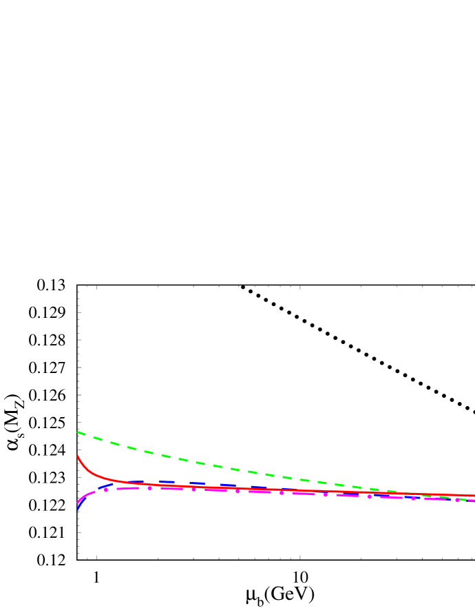
Figure 2: $\mu_{b}$ dependence of $\alpha_{s}^{(5)}(M_{Z})$ calculated from $\alpha_{s}^{(4)}(M_{\tau})=0.36$ and $M_{b}=4.7$ GeV. The procedure is described in the text. The dotted, short-dashed, long-dashed and dash-dotted line corresponds to one- to four-loop running. The solid curve includes the effect of the new four-loop matching term.

4 Effective coupling between a Higgs boson and gluons

In this Section we want to discuss the relation between $\zeta_{g}$ and the coupling of a scalar Higgs boson to gluons. Due to the fact that gluons are massless, there is no coupling at tree-level. At one-loop order the $HGG$ coupling is mediated via a top-quark loop depicted in Fig. 1(d).

For an intermediate-mass Higgs boson which formally obeys the relation $M_{H}\ll m_{t}$ it is possible to construct an effective Lagrangian of the form

$${\cal L}_{\rm eff} = -\frac{H^{0}}{v^{0}}C_{1}{\cal O}_{1}\,,$$ (14)

with the effective operator

$${\cal O}_{1} = \left(G^{a}_{\mu\nu}\right)^{2}\,,$$ (15)

where $G_{\mu\nu}^{a}$ is the colour field strength. The coefficient function $C_{1}$ incorporates the contribution from the top-quark loops. At one-loop order it is easy to see that the contribution from the triangle diagrams can be obtained through the derivative of the one-loop diagram for $\Pi_{G}^{0}$ with respect to the top-quark mass. However, at higher-loop orders this simple picture does not hold anymore and the relation between the $HGG$ diagrams and derivatives of the two-point functions containing a top-quark loop gets more involved. In Ref. [10] an all-order low-energy theorem has been derived which establishes such a relation and which has a surprisingly simple form (for definiteness we specify to the top-quark in this Section):

$$C_{1} = -\frac{1}{2}\,\frac{m_{t}^{2}\partial}{\partial m_{t}^{2}}\,\ln\zeta_{g}^{2}\,.$$ (16)

An appealing feature of Eq. (16) is that at a given order in $\alpha_{s}$ only the logarithmic contributions of $\zeta_{g}$ are needed for the calculation of $C_{1}$ at the same order. Thus, from our calculation we can reconstruct the five-loop logarithms of $\zeta_{g}$ from lower-order terms and the $\beta$ and $\gamma_{m}$ functions governing the running of $\alpha_{s}$ and the top-quark mass, respectively. This leads to the following result, at $N_{c}=3$ and $n_{h}=1$,

$$C_{1} = -\frac{1}{12}\,\frac{\alpha_{s}^{(n_{l}+1)}(\mu)}{\pi}\Bigg{\{}1+\frac{\alpha_{s}^{(n_{l}+1)}(\mu)}{\pi}\left(\frac{11}{4}-\frac{1}{6}\ln\frac{\mu^{2}}{m_{t}^{2}}\right)$$ (17)

$${}+\left(\frac{\alpha_{s}^{(n_{l}+1)}(\mu)}{\pi}\right)^{2}\Bigg{[}\frac{2821}{288}-\frac{3}{16}\ln\frac{\mu^{2}}{m_{t}^{2}}+\frac{1}{36}\ln^{2}\frac{\mu^{2}}{m_{t}^{2}}+n_{l}\left(-\frac{67}{96}+\frac{1}{3}\ln\frac{\mu^{2}}{m_{t}^{2}}\right)\Bigg{]}$$

$${}+\left(\frac{\alpha_{s}^{(n_{l}+1)}(\mu)}{\pi}\right)^{3}\Bigg{[}-\frac{4004351}{62208}+\frac{1305893}{13824}\zeta(3)-\frac{859}{288}\ln\frac{\mu^{2}}{m_{t}^{2}}+\frac{431}{144}\ln^{2}\frac{\mu^{2}}{m_{t}^{2}}-\frac{1}{216}\ln^{3}\frac{\mu^{2}}{m_{t}^{2}}$$

$${}+n_{l}\left(\frac{115607}{62208}-\frac{110779}{13824}\zeta(3)+\frac{641}{432}\ln\frac{\mu^{2}}{m_{t}^{2}}+\frac{151}{288}\ln^{2}\frac{\mu^{2}}{m_{t}^{2}}\right)$$

$${}+n_{l}^{2}\left(-\frac{6865}{31104}+\frac{77}{1728}\ln\frac{\mu^{2}}{m_{t}^{2}}-\frac{1}{18}\ln^{2}\frac{\mu^{2}}{m_{t}^{2}}\right)\Bigg{]}$$

$${}+\left(\frac{\alpha_{s}^{(n_{l}+1)}(\mu)}{\pi}\right)^{4}\Bigg{[}-\frac{69820734619}{27993600}-\frac{39407017}{373248}\ln^{4}2+\frac{11011}{8640}\ln^{5}2+\frac{39407017}{62208}\zeta(2)\ln^{2}2$$

$${}-\frac{11011}{864}\zeta(2)\ln^{3}2+\frac{27642438179}{24883200}\zeta(3)+\frac{996205247}{622080}\zeta(4)-\frac{187187}{1152}\zeta(4)\ln 2-\frac{894391}{4608}\zeta(5)$$

$${}-\frac{39407017}{15552}a_{4}-\frac{11011}{72}a_{5}+\frac{1967797}{622080}X_{0}$$

$${}-\left(\frac{1276661933}{1492992}-\frac{226222121}{331776}\zeta(3)\right)\ln\frac{\mu^{2}}{m_{t}^{2}}+\frac{33517}{1728}\ln^{2}\frac{\mu^{2}}{m_{t}^{2}}+\frac{140357}{20736}\ln^{3}\frac{\mu^{2}}{m_{t}^{2}}+\frac{1}{1296}\ln^{4}\frac{\mu^{2}}{m_{t}^{2}}$$

$${}+n_{l}\left(\frac{58259821853}{195955200}+\frac{3896297}{580608}\ln^{4}2-\frac{121}{1440}\ln^{5}2-\frac{3896297}{96768}\zeta(2)\ln^{2}2+\frac{121}{144}\zeta(2)\ln^{3}2\right.$$

$${}\left.-\frac{74306021071}{348364800}\zeta(3)+\frac{141211087}{3870720}\zeta(4)+\frac{2057}{192}\zeta(4)\ln 2-\frac{20227}{2304}\zeta(5)+\frac{3896297}{24192}a_{4}+\frac{121}{12}a_{5}\right.$$

$${}\left.-\frac{151369}{725760}X_{0}+\left(\frac{23250409}{186624}-\frac{8736121}{82944}\zeta(3)\right)\ln\frac{\mu^{2}}{m_{t}^{2}}+\frac{569}{2304}\ln^{2}\frac{\mu^{2}}{m_{t}^{2}}+\frac{2551}{2592}\ln^{3}\frac{\mu^{2}}{m_{t}^{2}}\right)$$

$${}+n_{l}^{2}\left(-\frac{33014371}{8957952}+\frac{685}{41472}\ln^{4}2-\frac{685}{6912}\zeta(2)\ln^{2}2+\frac{970259}{110592}\zeta(3)-\frac{518509}{55296}\zeta(4)\right.$$

$${}\left.+\frac{115}{192}\zeta(5)+\frac{685}{1728}a_{4}-\left(\frac{1107181}{186624}-\frac{28297}{9216}\zeta(3)\right)\ln\frac{\mu^{2}}{m_{t}^{2}}-\frac{1729}{13824}\ln^{2}\frac{\mu^{2}}{m_{t}^{2}}-\frac{1205}{5184}\ln^{3}\frac{\mu^{2}}{m_{t}^{2}}\right)$$

$${}+n_{l}^{3}\left(-\frac{255947}{1492992}+\frac{5}{64}\zeta(3)+\frac{481}{5184}\ln\frac{\mu^{2}}{m_{t}^{2}}-\frac{77}{6912}\ln^{2}\frac{\mu^{2}}{m_{t}^{2}}+\frac{1}{108}\ln^{3}\frac{\mu^{2}}{m_{t}^{2}}\right)$$

$${}+6\left(\beta_{4}^{(n_{l})}-\beta_{4}^{(n_{l}+1)}\right)\Bigg{]}+{\cal O}\left(\left(\frac{\alpha_{s}^{(n_{l}+1)}(\mu)}{\pi}\right)^{5}\right)\Bigg{\}}\,,$$

with $m_{t}$ being the $\overline{\rm MS}$ top-quark mass renormalized at the scale $\mu$. Note the appearance of the flavour-dependent part of $\beta_{4}$ in the five-loop contribution, whereas the corresponding coefficient from the anomalous mass dimension does not appear. We want to stress that the term of order $\alpha_{s}^{5}$ covers the contributions from five-loop diagrams like the one in Fig. 1(e).

Evaluating Eq. (17) numerically leads to

$$C_{1} \approx -\frac{1}{12}\,\frac{\alpha_{s}^{(n_{l}+1)}(m_{t})}{\pi}\Bigg{[}1+2.7500\,\frac{\alpha_{s}^{(n_{l}+1)}(m_{t})}{\pi}+\left(9.7951-0.6979\,n_{l}\right)\left(\frac{\alpha_{s}^{(n_{l}+1)}(m_{t})}{\pi}\right)^{2}$$ (18)

$$\mbox{}+\left(49.1827-7.7743\,n_{l}-0.2207\,n_{l}^{2}\right)\left(\frac{\alpha_{s}^{(n_{l}+1)}(m_{t})}{\pi}\right)^{3}$$

$$\mbox{}+\left(-662.5065+137.6005\,n_{l}-2.5367\,n_{l}^{2}-0.0775\,n_{l}^{3}+6\left(\beta_{4}^{(n_{l})}-\beta_{4}^{(n_{l}+1)}\right)\right)$$

$$\mbox{}\times\left(\frac{\alpha_{s}^{(n_{l}+1)}(m_{t})}{\pi}\right)^{4}\Bigg{]}\,.$$

Again one observes large cancellations between the $n_{l}^{0}$ and $n_{l}^{1}$ term in the five-loop contribution to $C_{1}$.

Note that the result of Eq. (17) constitutes a building block for the N⁴LO calculation to the Higgs boson production and decay in the two-gluon channel, for which the complete answer currently is certainly out of range. Still, the five-loop result for $C_{1}$ constitutes a high-order result in perturbative QCD which is of theoretical interest by itself.

5 Conclusions

In this paper the decoupling constant of the strong coupling is presented to four-loop order. This constitutes a fundamental quantity of QCD and is one of the very few known to such a high order. The decoupling constant is necessary for performing a consistent running of $\alpha_{s}$ with five-loop accuracy including important effects from the crossing of quark thresholds. The calculation has been performed analytically, and the main result can be found in Eq. (10). With the help of a low-energy theorem it is possible to derive the five-loop result for the effective coupling of the Higgs boson to gluons, which constitutes a building block in the corresponding production and decay processes.

We want to mention that the result for $\zeta_{g}^{2}$ in Eq. (10) has been obtained independently in Ref. [19]. Except for QGRAF, which is used for the generation of the diagrams, there is no common code. Even the master integrals have meanwhile been computed independently [20] and for the renormalization a different procedure has been chosen.

Acknowledgements
This work was supported by the SFB/TR 9. We would like to thank the authors of Ref. [19] for communicating their result before publication.

Appendix A Results for $\zeta_{g}^{\rm OS}$

Replacing in Eq. (10) the $\overline{\rm MS}$ mass $m_{h}$ by the pole mass $M_{h}$ using the three-loop approximation [21, 22, 23] one gets

$$\left(\zeta_{g}^{\rm OS}\right)^{2} = 1+\frac{\alpha_{s}^{(n_{l}+1)}(\mu)}{\pi}\left(-\frac{1}{6}\ln\frac{\mu^{2}}{M_{h}^{2}}\right)+\left(\frac{\alpha_{s}^{(n_{l}+1)}(\mu)}{\pi}\right)^{2}\left(-\frac{7}{24}-\frac{19}{24}\ln\frac{\mu^{2}}{M_{h}^{2}}+\frac{1}{36}\ln^{2}\frac{\mu^{2}}{M_{h}^{2}}\right)$$ (19)

$${}+\left(\frac{\alpha_{s}^{(n_{l}+1)}(\mu)}{\pi}\right)^{3}\left[-\frac{58933}{124416}-\frac{2}{3}\zeta(2)-\frac{2}{9}\zeta(2)\ln 2-\frac{80507}{27648}\zeta(3)-\frac{8521}{1728}\ln\frac{\mu^{2}}{M_{h}^{2}}\right.$$

$${}\left.-\frac{131}{576}\ln^{2}\frac{\mu^{2}}{M_{h}^{2}}-\frac{1}{216}\ln^{3}\frac{\mu^{2}}{M_{h}^{2}}+n_{l}\left(\frac{2479}{31104}+\frac{1}{9}\zeta(2)+\frac{409}{1728}\ln\frac{\mu^{2}}{M_{h}^{2}}\right)\right]$$

$${}+\left(\frac{\alpha_{s}^{(n_{l}+1)}(\mu)}{\pi}\right)^{4}\Bigg{[}-\frac{141841753}{24494400}+\frac{3179149}{1306368}\ln^{4}2-\frac{121}{4320}\ln^{5}2-\frac{697121}{19440}\zeta(2)$$

$${}+\frac{1027}{162}\zeta(2)\ln 2-\frac{2913037}{217728}\zeta(2)\ln^{2}2+\frac{121}{432}\zeta(2)\ln^{3}2-\frac{2408412383}{87091200}\zeta(3)$$

$${}+\frac{1439}{216}\zeta(3)\zeta(2)-\frac{71102219}{2177280}\zeta(4)+\frac{2057}{576}\zeta(4)\ln 2+\frac{49309}{20736}\zeta(5)$$

$${}+\frac{3179149}{54432}a_{4}+\frac{121}{36}a_{5}-\frac{151369}{2177280}X_{0}$$

$${}-\left(\frac{19696909}{746496}+\frac{29}{9}\zeta(2)+\frac{29}{27}\zeta(2)\ln 2+\frac{2439119}{165888}\zeta(3)\right)\ln\frac{\mu^{2}}{M_{h}^{2}}-\frac{7693}{1152}\ln^{2}\frac{\mu^{2}}{M_{h}^{2}}$$

$${}-\frac{8371}{10368}\ln^{3}\frac{\mu^{2}}{M_{h}^{2}}+\frac{1}{1296}\ln^{4}\frac{\mu^{2}}{M_{h}^{2}}+n_{l}\left(\frac{1773073}{746496}+\frac{173}{124416}\ln^{4}2+\frac{557}{162}\zeta(2)\right.$$

$$\left.{}+\frac{22}{81}\zeta(2)\ln 2-\frac{1709}{20736}\zeta(2)\ln^{2}2+\frac{4756441}{995328}\zeta(3)-\frac{697709}{165888}\zeta(4)+\frac{115}{576}\zeta(5)+\frac{173}{5184}a_{4}\right.$$

$$\left.{}+\left(\frac{1110443}{373248}+\frac{41}{54}\zeta(2)+\frac{2}{27}\zeta(2)\ln 2+\frac{132283}{82944}\zeta(3)\right)\ln\frac{\mu^{2}}{M_{h}^{2}}+\frac{6661}{10368}\ln^{2}\frac{\mu^{2}}{M_{h}^{2}}\right.$$

$$\left.{}+\frac{107}{1728}\ln^{3}\frac{\mu^{2}}{M_{h}^{2}}\right)+n_{l}^{2}\left(-\frac{140825}{1492992}-\frac{13}{162}\zeta(2)-\frac{19}{1728}\zeta(3)\right.$$

$$\left.{}-\left(\frac{1679}{186624}+\frac{1}{27}\zeta(2)\right)\ln\frac{\mu^{2}}{M_{h}^{2}}-\frac{493}{20736}\ln^{2}\frac{\mu^{2}}{M_{h}^{2}}\right)\Bigg{]}$$

$$\approx 1-0.2917\left(\frac{\alpha_{s}^{(n_{l}+1)}(M_{h})}{\pi}\right)^{2}+\left(-5.3239+0.2625\,n_{l}\right)\left(\frac{\alpha_{s}^{(n_{l}+1)}(M_{h})}{\pi}\right)^{3}$$

$${}+\left(-85.8750+9.6923\,n_{l}-0.2395\,n_{l}^{2}\right)\left(\frac{\alpha_{s}^{(n_{l}+1)}(M_{h})}{\pi}\right)^{4}\,.$$

References

[1]
P. A. Baikov, K. G. Chetyrkin and J. H. Kühn,
Phys. Rev. Lett. 95 (2005) 012003
[hep-ph/0412350].
[2]
Y. Schröder,
Nucl. Phys. Proc. Suppl. 116 (2003) 402
[hep-ph/0211288].